Angular Correlation of Gamma Rays 1. Angular Correlation

Copyright 2008, University of Chicago, Department of Physics

1

Angular Correlation of Gamma Rays

1. Angular Correlation of Pair-Annihilation Gamma Rays (P 211 and 334)

1.1 Introduction

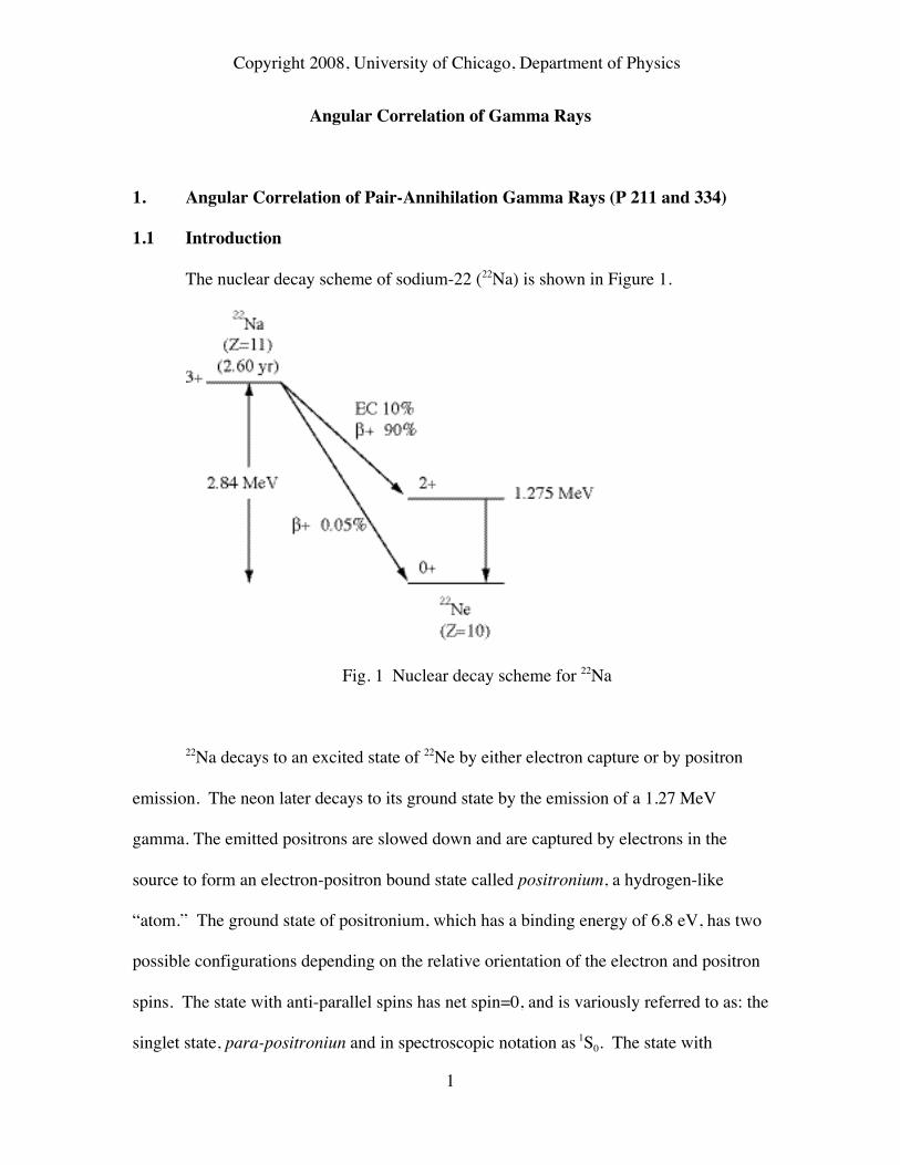
The nuclear decay scheme of sodium-22 (22Na) is shown in Figure 1.

Fig. 1 Nuclear decay scheme for 22Na

22Na decays to an excited state of 22Ne by either electron capture or by positron

emission. The neon later decays to its ground state by the emission of a 1.27 MeV

gamma. The emitted positrons are slowed down and are captured by electrons in the

source to form an electron-positron bound state called positronium, a hydrogen-like

“atom.” The ground state of positronium, which has a binding energy of 6.8 eV, has two

possible configurations depending on the relative orientation of the electron and positron

spins. The state with anti-parallel spins has net spin=0, and is variously referred to as: the

singlet state, para-positroniun and in spectroscopic notation as 1S0. The state with


2

parallel spins has net spin=1, and is referred to as: the triplet state, ortho-positronium

denoted by 3S1. The para- and ortho- states are both short-lived, but decay (by means of

electron-positron annihilation) with very different life times. Para-positronium has a

mean lifetime of about 10−10 s and decays to two photons. Ortho-positronium has a mean

lifetime of about 10−7 s and decays to 3 photons.

Question 1:

Why does the singlet state decay to two photons and the triplet state decay to

three photons?

Question 2:

Is it possible for either positronium state to decay to one photon?

Each state will be equally populated, so there will be three times as many

positronium “atoms” in the triplet state as in the singlet state. Therefore, one would

naively expect 3 times as many 3γ decays as 2γ decays. However, that is not what is

observed! Another process contributes to the actual outcome: a photon may be absorbed

by the electron in positronium, causing the electron to flip its spin, thus changing the state

of the positronium from ortho- to para- or vice versa. The lifetime for the spin flip

process is about 10−9 s, long compared to the para- lifetime but short compared to the

ortho- lifetime. Thus, para-positronium decays (via 2 photons) before a spin flip can

occur. Whereas, spin flips occur before ortho-positronium has time to decay (via 3


3

photons), converting the ortho- to para-. The para- thus created also decays via 2 photon

decay. Therefore, the 2 photon decay is much more likely.

Since the rest masses m0 of the electron and positron are converted to energy in

the annihilation process, each of the resulting two photons has energy E = m0c2 =511-

keV, and are created simultaneously.

Question 3:

If the positronium is at rest in the lab frame when annihilation takes place, in what

relative directions must the two photons be emitted?

1.2 Apparatus

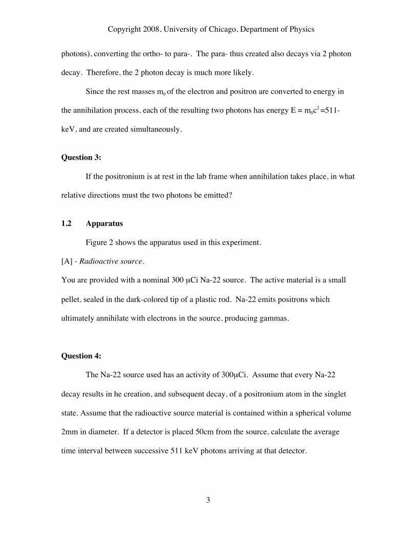
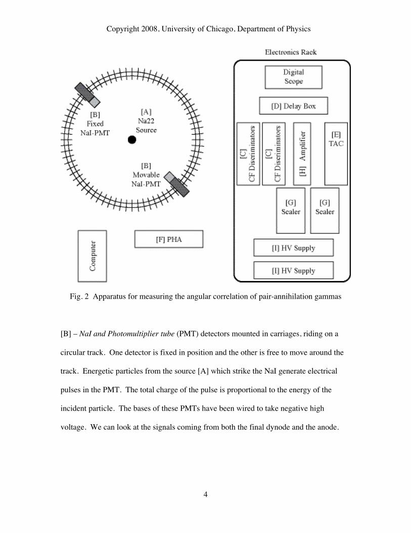
Figure 2 shows the apparatus used in this experiment.

[A] - Radioactive source.

You are provided with a nominal 300 µCi Na-22 source. The active material is a small

pellet, sealed in the dark-colored tip of a plastic rod. Na-22 emits positrons which

ultimately annihilate with electrons in the source, producing gammas.

Question 4:

The Na-22 source used has an activity of 300µCi. Assume that every Na-22

decay results in he creation, and subsequent decay, of a positronium atom in the singlet

state. Assume that the radioactive source material is contained within a spherical volume

2mm in diameter. If a detector is placed 50cm from the source, calculate the average

time interval between successive 511 keV photons arriving at that detector.


4

Fig. 2 Apparatus for measuring the angular correlation of pair-annihilation gammas

[B] – NaI and Photomultiplier tube (PMT) detectors mounted in carriages, riding on a

circular track. One detector is fixed in position and the other is free to move around the

track. Energetic particles from the source [A] which strike the NaI generate electrical

pulses in the PMT. The total charge of the pulse is proportional to the energy of the

incident particle. The bases of these PMTs have been wired to take negative high

voltage. We can look at the signals coming from both the final dynode and the anode.


5

Question 5:

What is the expected polarity of the dynode and anode pulses?

For more details on how these detectors work see, for example, Radiation Detection and

Measurement, by Glenn Knoll.

[C] - Constant fraction (CF) discriminators. The output pulses from the detectors are

sent to the input of the CF discriminators. The CF discriminators generate an output

pulse only if the voltage of the input pulse is within an upper and lower limit set by the

user.

[D] - Analog time delay. This box used coaxial cable of different lengths to delay pulses

by different times. Delay times of up to 60ns are set by toggle switches

[E] - Time to Amplitude Converter (TAC). The TAC has start and stop inputs. A start

pulse initiates a linearly increasing voltage ramp in the TAC. The ramp stops increasing

when either a pulse arrives at the stop input, or a preset time limit (range) is exceeded. If

a stop pulse arrives before the range is reached, the TAC generates an output pulse whose

voltage is proportional to the time between the start and stop pulses. If the range is

exceeded the TAC resets itself and produces no output pulse.


6

[F] - Pulse Height Analyzer (PHA). The PHA integrates the charge in each pulse

(proportional to energy of the gamma) and displays a histogram of pulse charges on a

computer. For more detailed information on how to operate the PHA see the appendix.

[G] - Scalers. A scaler counts pulses.

[H] - Amplifier. Used here to amplify dynode pulses from the PMTs.

[I] - High Voltage (HV) Supply. Each PMT is powered by a separate HV supply. The

PMT's in this experiment can be safely run up to -2500V.

1.3 Method

Since our model for electron-positron annihilation assumes the simultaneous

creation of two 511 keV photons, we wish to set up our detection and counting system to

look for coincident events at 511 keV. Then we will measure the counting rate for those

events as a function of angle between the two detectors.

1.4 Procedure

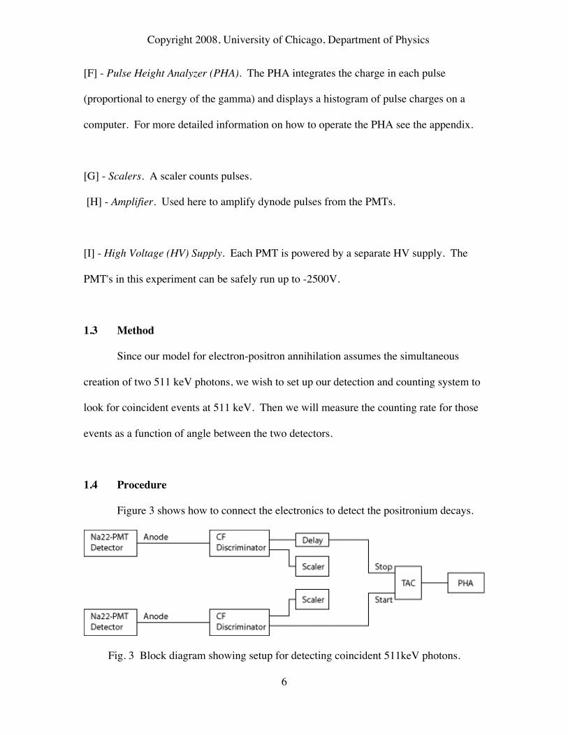
Figure 3 shows how to connect the electronics to detect the positronium decays.

Fig. 3 Block diagram showing setup for detecting coincident 511keV photons.


7

Use coaxial cable to connect the PMT anodes to the inputs of the CF

discriminators. The upper and lower level thresholds of the CF discriminators must be

set so that only pulses from 511 keV photons will generate an output pulse. In this way

we can reject unwanted background events, such as the 1.27 MeV photons from the Na22

decay. One output from each CF discriminator is sent to a scaler so that the rate of 511

keV events can be measured for each detector. These rates are often referred to as the

singles rates. A second output from one of the CF discriminators, it does not matter

which, is connected to the start input of the TAC. A second output from the other CF

discriminator is sent through the delay box and then into the stop input of the TAC.

Thus, 511 keV photons which hit the two detectors simultaneously will produce start and

stop pulses at the TAC separated by a time equal to the added delay on the stop channel.

Question 6:

Why is it necessary to add delay time to the stop channel? Hint, what would be

the output of the TAC for simultaneous detector events if there were no delay.

The following sections will walk you through setting up the electronics. Before

proceeding, make sure you understand what the pulses from the PMT should look like

and what pulse height spectra (PHS) you expect to see from a monochromatic source.

At each output through the chain of electronics you should look at the pulses on

the scope and sketch what you see into your lab notebook. Include measurements of

voltages and times for each sketch. These observations are an important part of setting

up the electronics for experiments using this type of electronics modules.


8

1.4.1 Setting the PMT high voltage

Set both HV supplies to negative polarity at -2000V. Turn on the HV supplies as

follows: Start with both switches on each supply turned off. Flip on the left-hand switch.

After about 30 seconds you will hear a click and the power light will come on. Now flip

the standby switch on and look for a negative deflection of the meter. The PMTs should

now be powered.

With a Na-22 rod source mounted in the center of the table, start by looking at the

anode and dynode pulses from one of the PMTs on the scope at the same time. Use a

50Ω terminator at each scope input.

Question 7:

Why is the 50Ω terminator necessary?

Set both channels of the scope to the same voltage and time scale. Sketch the pulses in

your lab notebook, recording the voltages and times.

Question 8:

Why are the pulses different polarity? Why are they not the same pulse height?

Now look at the anode pulses from both PMTs on the scope at the same time. If

the average pulse heights from the two PMTs are very different adjust their HV. Don't

exceed -2500V!


9

1.4.2 Obtain a Na-22 spectrum

Connect the dynode of one of the PMTs to the amplifier. Connect the output of

the amplifier to the direct input of the PHA. Use the SpecTech software on the computer

to collect a pulse height spectrum of the dynode pulses. Refer to the appendix for details

on how to operate the SpecTech software.

Adjust the gain of the amplifier until the spectrum shows peaks for both the 511

keV and the 1.27 MeV gammas expected from the decay of Na-22. You should see the

full energy peak and Compton shelf associated with each of the two energies. The idea is

to get the full pulse height spectrum displayed on the PHA so that you can determine

which part of the spectrum represents the 511 keV photons.

Question 9:

Make a plot of the spectrum of Na-22. Identify the 511KeV photopeak and

explain why you believe you have identified the correct peak in the spectrum.

1.4.3 Gating the PHA

In the next section we wish to have visual feedback to select the relevant portion

of the spectrum. We will make use the PHA gate input to set the criterion for which

pulses will be analyzed. A pulse arriving at the direct input of the PHA will be analyzed

only if another pulse arrives simultaneously at the gate input.

For the gating system to work properly, the amplified dynode pulse must arrive

within the time bracketed by the gate pulse. To check this timing, connect the dynode

output of one of the PMTs to the amplifier and the output of the amplifier to one channel


10

of the scope. Locate the CF discriminator which is connected to the anode of the same

PMT. Connect the SCA out (rear of CF discriminator) to the other channel of the scope.

The SCA Out pulse is generated along with every output pulse from the CF

discriminator. Look at the SCA Out and the amplified Dynode pulses on the scope at the

same time. Sketch them in your lab book.

Question 10:

Do the dynode pulses appear within the time window defined by the SCA Out

pulses?

1.4.4 Selecting the 511 keV peak

We wish to count only the relevant 511 keV annihilation photons. This can be

accomplished by adjusting the upper and lower levels on the CF discriminators so that

only pulses in the 511 keV photopeak portion of the spectrum will be accepted. The

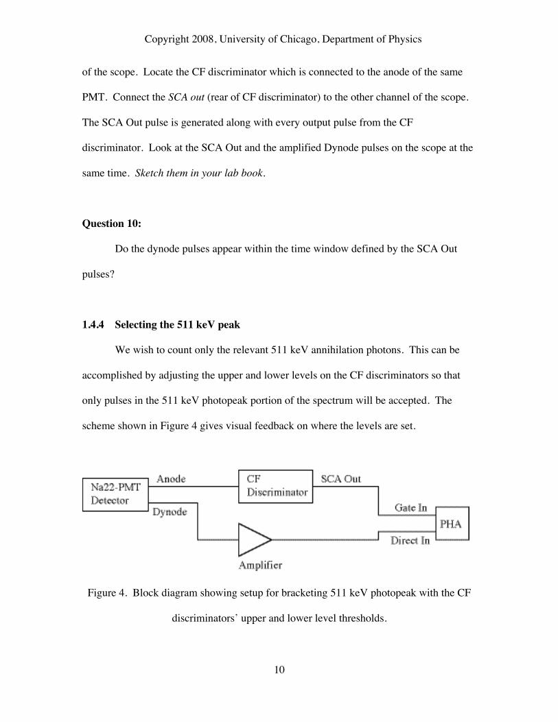
scheme shown in Figure 4 gives visual feedback on where the levels are set.

Figure 4. Block diagram showing setup for bracketing 511 keV photopeak with the CF

discriminators’ upper and lower level thresholds.


11

For each detector in turn, make the connections shown in Fig. 4. On the

discriminators, gently adjust the upper level threshold to its maximum setting and the

lower level threshold to its minimum setting, thus allowing the maximum range of pulse

sizes to be accepted by the discriminators and generate an output pulse. At this point the

singles rates for both PMT's should be within a factor of 2 of each other.

Before continuing, look at the output of one of the CF discriminators on the

scope. Sketch the pulses in your lab notebook including details of the pulse heights and

widths. Note that although the input pulses to the CF discriminator vary in height,

according to the energy of the incident photon, the output pulses are all a standard height

and width. The standardized output pulse shape increases timing precision, but removes

pulse height information.

To obtain visual feedback on the effect of the upper and lower level threshold

settings on the spectrum we will use the system as shown in Fig. 4. In this scheme only

when an anode pulse gets through the discriminator’s voltage window and opens the gate,

do we allow the amplified dynode pulse to be analyzed. The PHA will now only count

pulses on the Direct input which arrive when there is also a pulse present on the "gate"

input. Start collecting data on the PHA. With the upper and lower level thresholds on

the CF discriminator fully open you should see the full spectrum of the Na-22 source,

including the full energy peaks of both the 511KeV and 1.27MeV gammas.

Now adjust the upper and lower level thresholds on the CF discriminator until

only the 511KeV full energy peak appears on the PHA. Note that the threshold controls

do not produce a sharp cut off in the spectrum. Try to adjust the thresholds as close as

possible to the 511KeV photopeak without reducing the rate at which they accumulate.


12

Repeat this procedure for the other PMT. Once you have adjusted the windows

on both discriminators, observe the rates of the output pulses. If the rates are

significantly different, readjust the threshold levels to make the rates more equal.

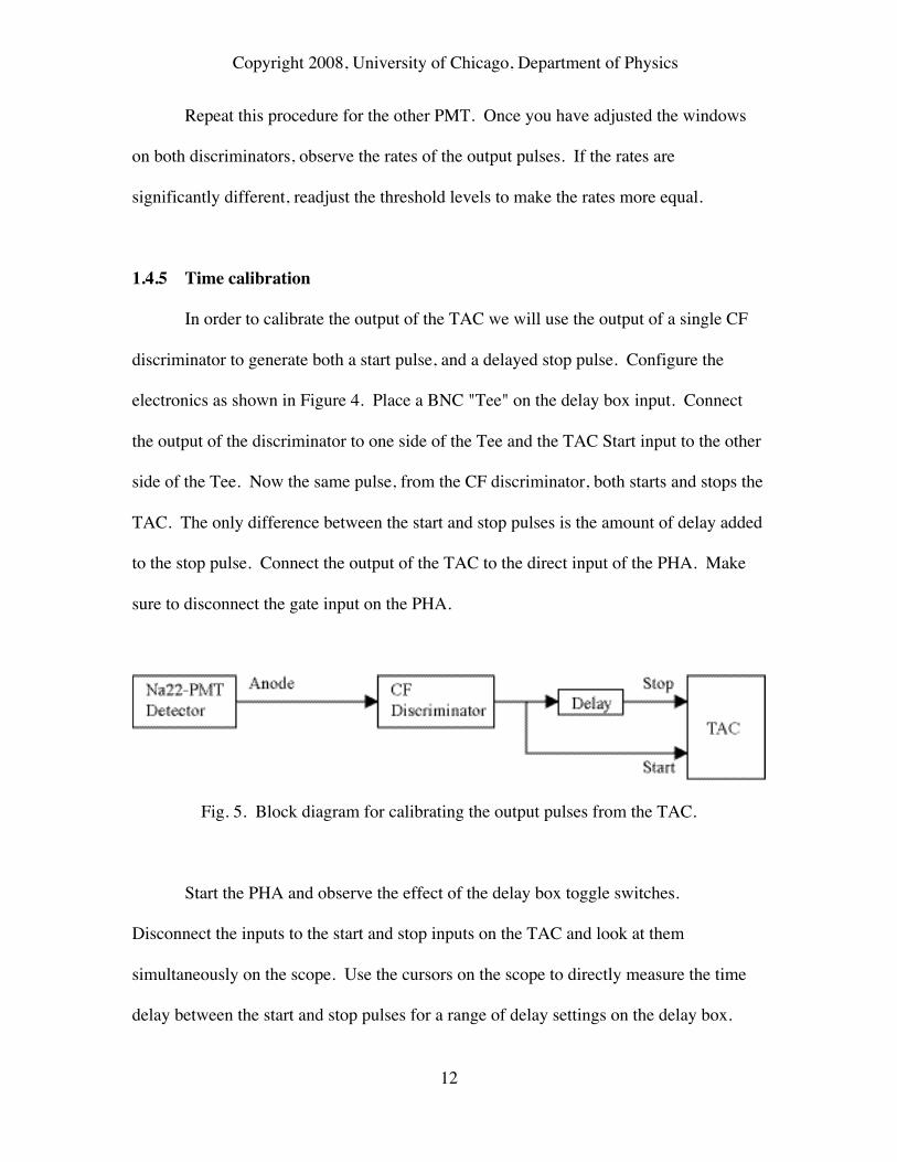
1.4.5 Time calibration

In order to calibrate the output of the TAC we will use the output of a single CF

discriminator to generate both a start pulse, and a delayed stop pulse. Configure the

electronics as shown in Figure 4. Place a BNC "Tee" on the delay box input. Connect

the output of the discriminator to one side of the Tee and the TAC Start input to the other

side of the Tee. Now the same pulse, from the CF discriminator, both starts and stops the

TAC. The only difference between the start and stop pulses is the amount of delay added

to the stop pulse. Connect the output of the TAC to the direct input of the PHA. Make

sure to disconnect the gate input on the PHA.

Fig. 5. Block diagram for calibrating the output pulses from the TAC.

Start the PHA and observe the effect of the delay box toggle switches.

Disconnect the inputs to the start and stop inputs on the TAC and look at them

simultaneously on the scope. Use the cursors on the scope to directly measure the time

delay between the start and stop pulses for a range of delay settings on the delay box.


13

Now reconnect the start and stop pulses to the TAC and use these settings to calibrate the

x-axis of the PHA in units of time.

1.5 Data collection and analysis

Reconnect the electronics according to Figure 3. Collect events from the TAC for

a range of detector angles θ around 180°. At each angle record the spectrum from the

TAC and the singles rate for each detector. Spend sufficient time on each data point to

accumulate a statistically significant number of counts.

Question 11:

How many counts do you need to obtain 3% statistics? 1% statistics? How much

is enough for your experiment?

Plot your data as you go and make sure you take data an enough angles to clearly define

the shape of the curve. Take one data point at an angle far from 180° to get a measure of

the accidental coincidence rate.

Question 12:

From the width of the TAC peak on the PHA, estimate the resolving time of the

experiment.


14

Question 13:

Using the singles rates and the system resolving time estimate the expected rate of

accidental coincidences. How does this rate compare with your measured accidental

coincidence rate?

Question 14:

From your coincidence rate vs. angle data and the geometry of the detectors,

deduce the angular distribution of the 511 keV gamma rays. Compare with the

theoretical prediction.

Question 15:

The positron decay of Na-22 is accompanied by the prompt emission of a 1.277

MeV gamma ray. The positrons come to rest and form positronium on a time scale of 10-

12 seconds. However the lifetime of the positronium atom is of order 10-9 seconds.

Discuss how you could go about measuring the lifetime of the positronium atoms with

the equipment at hand. Given what you know about the energy and time resolution of the

equipment, is this measurement feasible?

2. Angular correlation in Ni60 (Physics 334 only)

2.1 Introduction

Cobalt-60 decays to an excited state of nickel-60. Ni60 decays with the emission

of two, nearly simultaneous gammas (see the nuclear decay scheme for details). There is

a correlation between the direction of the nuclear spin axis and the direction of emission


15

of the gammas. The time between the emissions of the first and second gammas is so

short that the nuclear spin axis cannot appreciably change orientation during that time.

Thus, there is an angular correlation between the emission directions of the two gammas.

Theory tells us that the angular correlation of these gammas is coupled to the nuclear

decay mode.

Question 16:

Use the appropriate theory to predict all the possible decay modes for the decay of

Ni60 from its 4+ state to its ground state.

Question 17:

For each of the above decay modes, predict its angular correlation function.

2.2 Take data with Co60

Replace the Na22 source with the Co60 source and take data as you did earlier.

Since the expected angular distribution of coincident gammas is not necessarily sharply

peaked at 180 degrees as with Na22, it is necessary to take data over a broad range of

angles.

2.3 Data analysis

Repeat the data analysis as you did for Na22. Do a careful analysis of

uncertainties, statistical and systematic. Compare your measured angular correlation

function with those of the possible decay modes predicted by theory.


16

Question 18:

With what decay mode(s) are your data consistent?

Documents

Angular Correlation of Gamma Rays 1. Angular Correlation