ANGLE OF ARRIVAL(AOA)

By Rajarshi Biswas

B. Tech In CSE, 4th Year, 7th Semester

Roll-13000110012

INTRODUCTION

Awareness of the physical location for each node is required by many wireless sensor network

applications. The discovery of the position can be realized utilizing range measurements

including received signal strength, time of arrival, time difference of arrival and angle of arrival.

In this presentation, we focus on localization techniques based on angle of arrival information

between neighbour nodes.

The emergence of wireless sensor networks (WSNs) has facilitated our interaction with the physical

environment. A WSN consists of a large number of distributed sensor nodes, which are generally inexpensive

and resource constrained. The network is often configured such that the communication between the sensor

nodes and the base stations requires multiple hops. Such a network topology can be traced back to the

ancient defensive systems. Instead of using electronic sensors, in the past, beacon towers would send signals

(e.g., Beacon fires, flags, smoke and drums) upon the observation of enemy activity. The signals usually passed

through several towers before reaching the command centre. In contrast to this ancient system, modern WSNs

require no or minimal human attendance. In many WSN applications, including monitoring and tracking, the

data collected is meaningless without the positions of the corresponding sensor nodes. The positions can be

discovered either by equipping each sensor nodes with a global positioning system (GPS) or by hand-placing

the sensors. However, both are impractical for many WSN applications due to the expense in terms of cost and

human effort.

Another technique is to use a limited number of nodes that are aware of their. These nodes are referred to as

BEACONS. The rest of the nodes are referred to as unknowns and utilize beacons’ positions to localize

themselves.

LOCALIZATION IN WIRELESS SENSOR NETWORKS

• WHAT?

TO DETERMINE THE PHYSICAL COORDINATES OF A GROUP OF SENSOR NODES IN A WIRELESS SENSOR NETWORK (WSN)

DUE TO APPLICATION CONTEXT, USE OF GPS IS UNREALISTIC, THEREFORE, SENSORS NEED TO SELF-ORGANIZE A COORDINATE SYSTEM

• WHY?

TO REPORT DATA THAT IS GEOGRAPHICALLY MEANINGFUL

SERVICES SUCH AS ROUTING RELY ON LOCATION INFORMATION; GEOGRAPHIC ROUTING PROTOCOLS; CONTEXT-BASED ROUTING PROTOCOLS, LOCATION-AWARE SERVICES

LOCALIZATION IN WIRELESS SENSOR NETWORKS CONT.

IN GENERAL, ALMOST ALL THE SENSOR NETWORK LOCALIZATION

ALGORITHMS SHARE THREE MAIN PHASES:

DISTANCE ESTIMATION

POSITION COMPUTATION

LOCALIZATION ALGHORITHM

Depending on the mechanisms used, localization schemes can be

classified into two categories:

Range-free or proximity-based

Range-based.

LOCALIZATION IN WIRELESS SENSOR NETWORKS CONT.

THE DISTANCE ESTIMATION PHASE INVOLVES MEASUREMENT TECHNIQUES TO ESTIMATE

THE RELATIVE DISTANCE BETWEEN THE NODES.

THE POSITION COMPUTATION CONSISTS OF ALGORITHMS TO CALCULATE THE COORDINATES

OF THE UNKNOWN NODE WITH RESPECT TO THE KNOWN ANCHOR NODES OR OTHER

NEIGHBORING NODES.

THE LOCALIZATION ALGORITHM, IN GENERAL, DETERMINES HOW THE INFORMATION

CONCERNING DISTANCES AND POSITIONS, IS MANIPULATED IN ORDER TO ALLOW MOST OR

ALL OF THE NODES OF A WSN TO ESTIMATE THEIR POSITION. OPTIMALLY THE LOCALIZATION

ALGORITHM MAY INVOLVE ALGORITHMS TO REDUCE THE ERRORS AND REFINE THE NODE

POSITIONS.

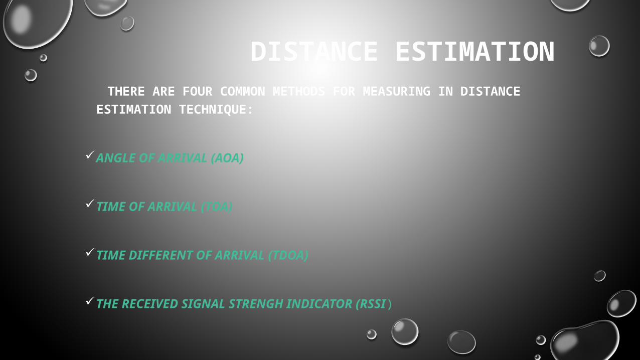
DISTANCE ESTIMATION THERE ARE FOUR COMMON METHODS FOR MEASURING IN DISTANCE ESTIMATION

TECHNIQUE:

ANGLE OF ARRIVAL (AOA)

TIME OF ARRIVAL (TOA)

TIME DIFFERENT OF ARRIVAL (TDOA)

THE RECEIVED SIGNAL STRENGH INDICATOR (RSSI)

ANGLE OF ARRIVAL Method Allows Each Sensor To Evaluate The Relative Angles Between Received Radio Signals.

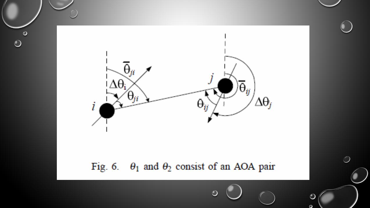
AOA is defined as the angle between the propagation direction of an incident wave and some reference direction, which is known as orientation.

Orientation, defined as a fixed direction against which the AOAs are measured, is represented in degrees in a clockwise direction from the north.

When The orientation is 0o or pointing to the north, the AOA is absolute, otherwise, relative. One common approach to obtain AOA measurements is to use an antenna array on each sensor node.

GSC-9, Seoul 11

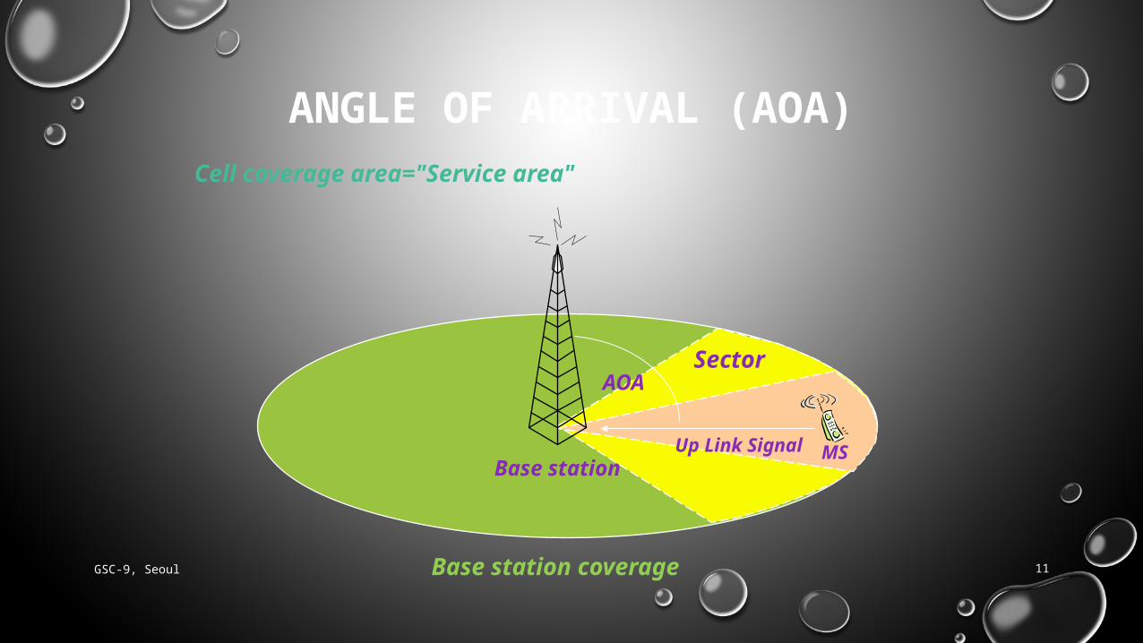
ANGLE OF ARRIVAL (AOA)Cell coverage area="Service area"

Base station coverage

Base station

Sector

MS

AOA

Up Link Signal

GSC-9, Seoul 12

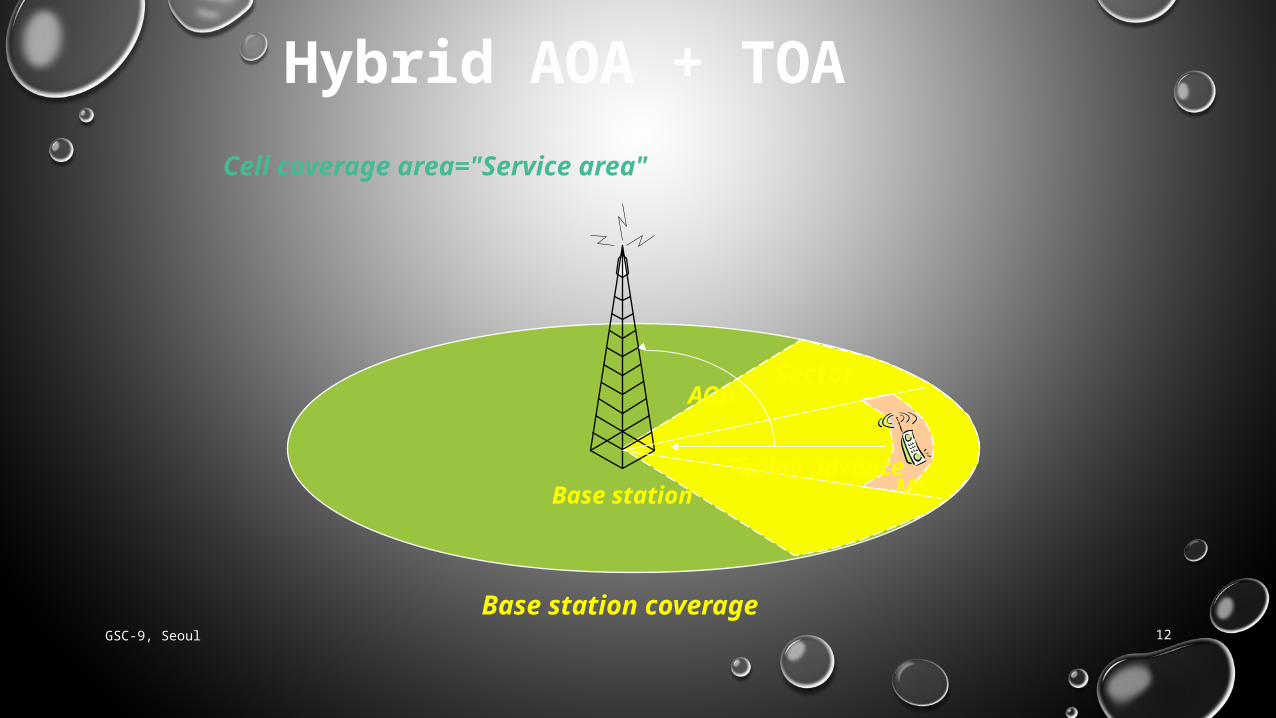
Hybrid AOA + TOA

Cell coverage area="Service area"

Base station

Base station coverage

Sector

MSTiming advance

AOA

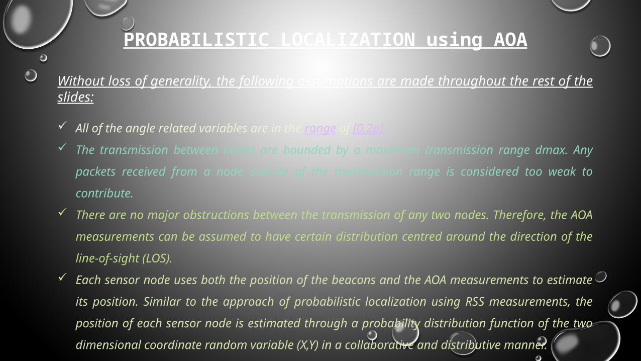
PROBABILISTIC LOCALIZATION using AOA

Without loss of generality, the following assumptions are made throughout the rest of the slides:

All of the angle related variables are in the range of [0,2p).

The transmission between nodes are bounded by a maximum transmission range dmax. Any packets

received from a node outside of the transmission range is considered too weak to contribute.

There are no major obstructions between the transmission of any two nodes. Therefore, the AOA

measurements can be assumed to have certain distribution centred around the direction of the line-of-

sight (LOS).

Each sensor node uses both the position of the beacons and the AOA measurements to estimate its

position. Similar to the approach of probabilistic localization using RSS measurements, the position of each

sensor node is estimated through a probability distribution function of the two dimensional coordinate

random variable (X,Y) in a collaborative and distributive manner.

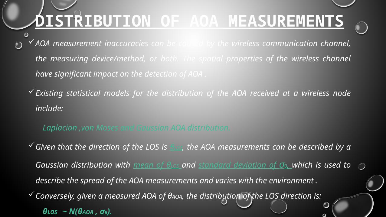
DISTRIBUTION OF AOA MEASUREMENTSAOA measurement inaccuracies can be caused by the wireless communication channel, the

measuring device/method, or both. The spatial properties of the wireless channel have

significant impact on the detection of AOA .

Existing statistical models for the distribution of the AOA received at a wireless node include:

Laplacian ,von Moses and Gaussian AOA distribution.

Given that the direction of the LOS is θLOS, the AOA measurements can be described by a

Gaussian distribution with mean of θLOS and standard deviation of σθ, which is used to describe

the spread of the AOA measurements and varies with the environment.

Conversely, given a measured AOA of θAOA, the distribution of the LOS direction is:

θLOS ~ N(θAOA , σθ).

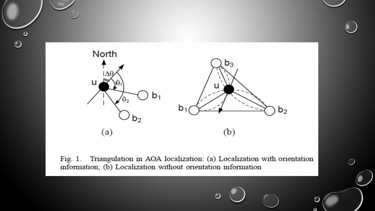
PROBABILISTIC LOCALIZATION WITH ORIENTATION INFORMATION

We refer to our approach as probabilistic because the positions (and later the orientations) are estimated through

probability distribution functions. The absolute AOA can be calculated using both the orientation information and the

relative AOA as depicted in fig. 1(a).

For an unknown with known orientation, the minimum number of neighbour beacons required to estimate the

position is two. However, since the nodes are usually assumed to be (very) sparse, most of the nodes can only hear

directly from one or no beacon, thus making localizations for them impossible. In the proposed approach, the

position information of beacons multiple hops away is used, such that the estimation can be performed at each node.

PROBABILISTIC LOCALIZATION WITH ORIENTATION INFORMATION CONT.

We define, a pseudo-beacon, as an unknown with an estimated position probability density function (pdf). To propagate

The position information of the beacons, both beacons and pseudo-beacons send out beacon packets to their one-hop

Neighbours. Initially, each unknown initiates its position to be uniformly distributed over the entire network deployment

Area. An unknown node j receiving a beacon packet from a beacon/pseudo-beacon node i executes the following steps:

Measures the relative AOAs of the received packets and calculates the absolute AOAs;

Updates its position distribution and pdf using both the position information of beacons/pseudo-beacons and the

Computed absolute AOAs;

All unknowns with updated pdfs become pseudo-beacons and send out their updated pdfs to their one-hop neighbours.

Assume the angle is j’s measured absolute AOA of i’s Beacon packet, according to (1), the distribution of i’s LOS Direction ‘seen’ at j is:

Variable Фij can be considered as the angular coordinate in the polar coordinate system. In

addition, we define distance random variable Dij , which represents the distance from node i to j.

Variables Фij and Dij are independent. In Order to

find the joint pdf fФij ,Dij(θ ,d), the pdf of Dij has to be determined. As we use only angle measurement, the only information about the distance between nodes i and j is that Dij ≤ dmax.

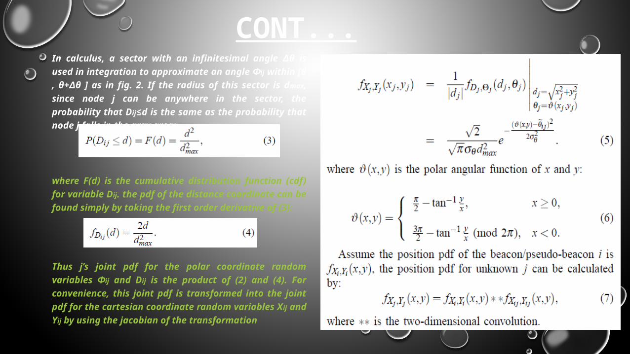
CONT...In calculus, a sector with an infinitesimal angle Δθ is used in integration to approximate an angle Фij within [θ , θ+Δθ ] as in fig. 2. If the radius of this sector is dmax, since node j can be anywhere in the sector, the probability that Dij≤d is the same as the probability that node j falls in the gray area:

where F(d) is the cumulative distribution function (cdf) for variable Dij. the pdf of the distance coordinate can be found simply by taking the first order derivative of (3):

Thus j’s joint pdf for the polar coordinate random variables Фij and Dij is the product of (2) and (4). For convenience, this joint pdf is transformed into the joint pdf for the cartesian coordinate random variables Xij and Yij by using the jacobian of the transformation

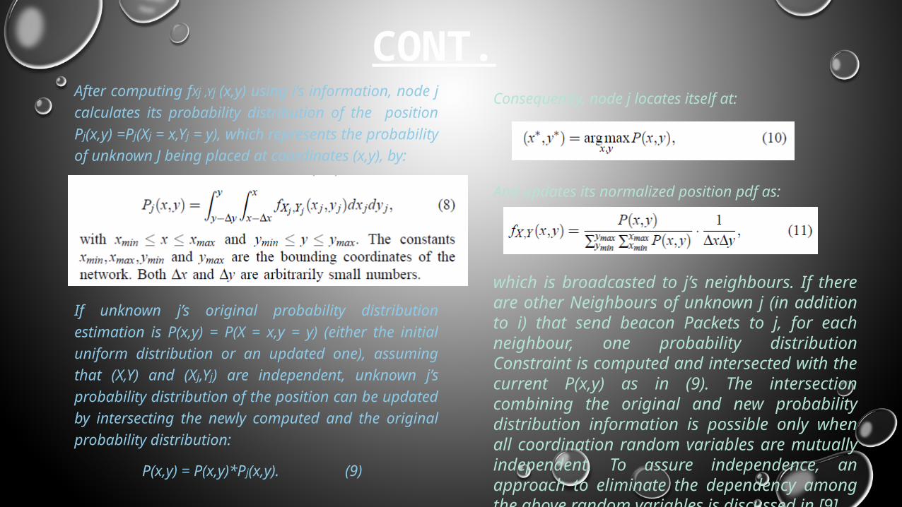
CONT.After computing fXj ,Yj (x,y) using i’s information, node j calculates its probability distribution of the position P j(x,y) =Pj(Xj = x,Yj = y), which represents the probability of unknown J being placed at coordinates (x,y), by:

If unknown j’s original probability distribution estimation is P(x,y) = P(X = x,y = y) (either the initial uniform distribution or an updated one), assuming that (X,Y) and (Xj,Yj) are independent, unknown j’s probability distribution of the position can be updated by intersecting the newly computed and the original probability distribution:

P(x,y) = P(x,y)*Pj(x,y). (9)

Consequently, node j locates itself at:

And updates its normalized position pdf as:

which is broadcasted to j’s neighbours. If there are other Neighbours of unknown j (in addition to i) that send beacon Packets to j, for each neighbour, one probability distribution Constraint is computed and intersected with the current P(x,y) as in (9). The intersection combining the original and new probability distribution information is possible only when all coordination random variables are mutually independent. To assure independence, an approach to eliminate the dependency among the above random variables is discussed in [9].

EXAMPLE

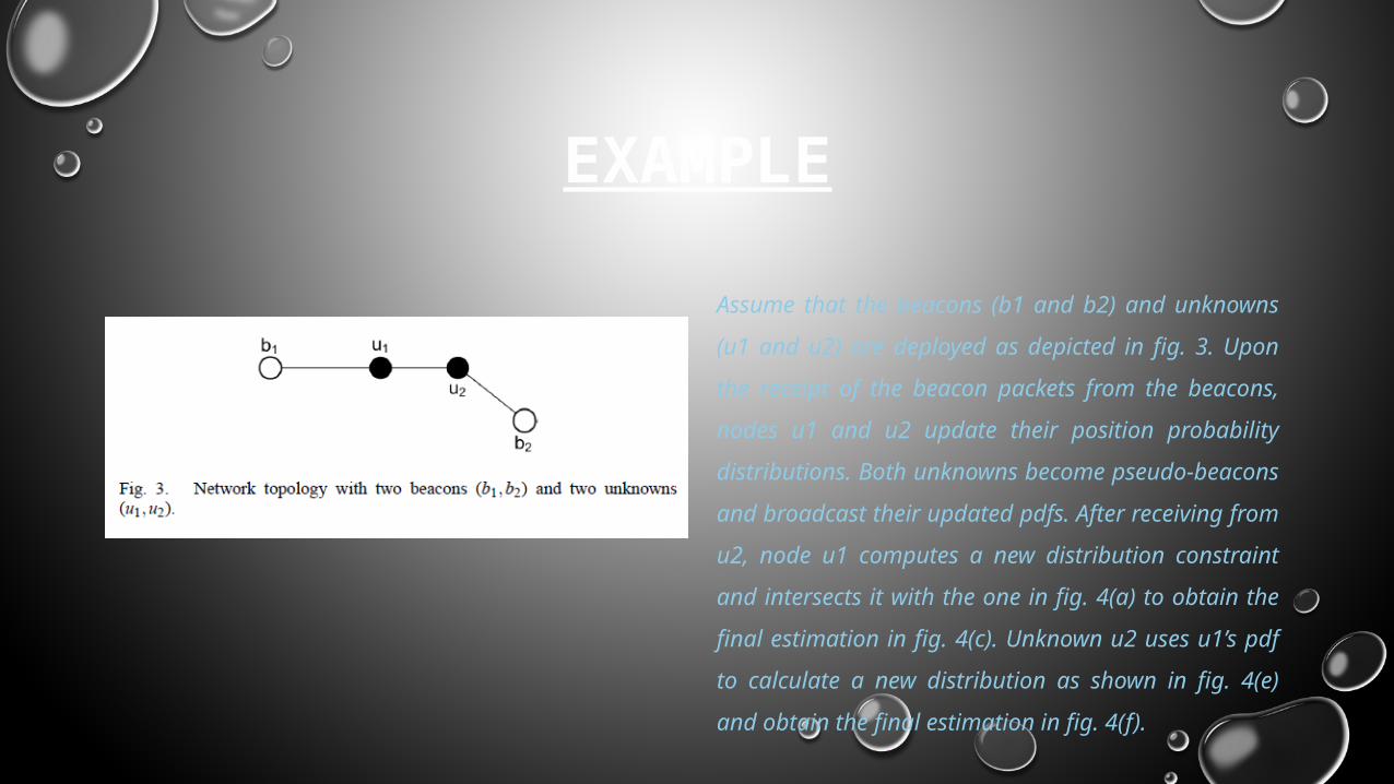
Assume that the beacons (b1 and b2) and unknowns (u1

and u2) are deployed as depicted in fig. 3. Upon the receipt

of the beacon packets from the beacons, nodes u1 and u2

update their position probability distributions. Both

unknowns become pseudo-beacons and broadcast their

updated pdfs. After receiving from u2, node u1 computes a

new distribution constraint and intersects it with the one in

fig. 4(a) to obtain the final estimation in fig. 4(c). Unknown

u2 uses u1’s pdf to calculate a new distribution as shown in

fig. 4(e) and obtain the final estimation in fig. 4(f).

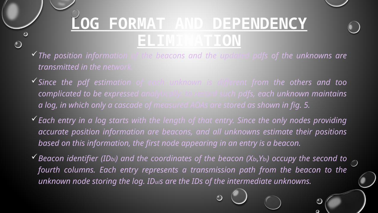
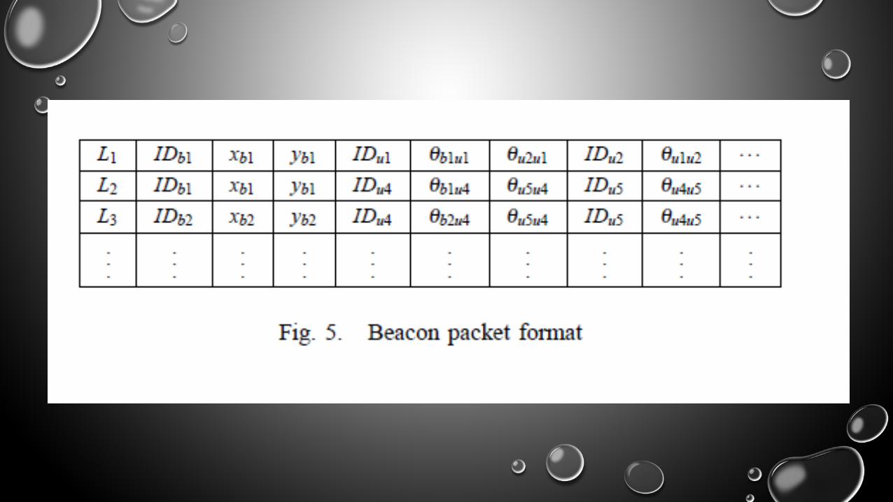
LOG FORMAT AND DEPENDENCY ELIMINATIONThe position information of the beacons and the updated pdfs of the unknowns are transmitted

in the network.

Since the pdf estimation of each unknown is different from the others and too complicated to be expressed analytically, to record such pdfs, each unknown maintains a log, in which only a cascade of measured AOAs are stored as shown in fig. 5.

Each entry in a log starts with the length of that entry. Since the only nodes providing accurate position information are beacons, and all unknowns estimate their positions based on this information, the first node appearing in an entry is a beacon.

Beacon identifier (IDbi) and the coordinates of the beacon (Xbi,Ybi) occupy the second to fourth columns. Each entry represents a transmission path from the beacon to the unknown node storing the log. IDuis are the IDs of the intermediate unknowns.

A beacon can be in multiple entries, as the first two entries shown in the table, since all neighbour unknowns

of the beacon relay its position information. Similarly, a single unknown can appear in multiple entries. Upon

the receipt of a beacon packet from a neighbour node, an intermediate unknown appends its node ID to the

packet entry and records two AOAs: one is the measured AOA of the incident packet from the ancestor node;

the other is the measured AOA of the next node along the path. If the orientations are known, the recorded

AOAs are absolute, otherwise, relative. Beacon packets from an unknown contain one to several entries from

that unknown’s log. Packets from beacon nodes follow the same format (but having only the beacon

information). Each destination unknown appends its ID and the measured AOA from its ancestor to the

packet, and stores the new packet in its log.

THE LOG….The log is then processed using the method introduced in [9] to eliminate the dependencies among entries. The processed log has the following properties to ensure the information in the log is independent [9]:

A node can appear only once in an entry.

If an intermediate unknown appears in more than one entry and occupies column ci in ith entry, then (Li−Ci) should be the same for all entries where the unknown appears. In other words, in all entries where the intermediate unknown appears, the number of hops between the intermediate unknown and the node storing the log (i.e., The node that estimates its position) must be the same.

If there is more than one entry containing a path starting from an intermediate unknown i to another intermediate unknown j, the nodes between i and j must be same.

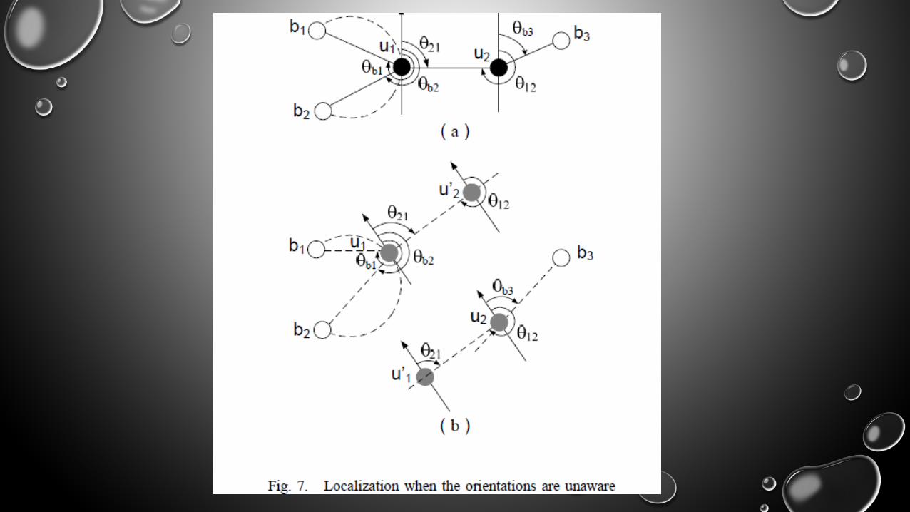
The processed log is then used at each unknown to estimate its position based on the approach when its orientation is known. When unknowns are not aware of their orientations, the processed logs are used to find both orientation and position.

CONCLUSION

In this presentation, we presented a distributed AOA-based localization and

orientation approach for wireless sensor networks under the assumption that all

unknown sensors are capable of detecting angles of the incident signal from the

neighbouring nodes. Even with inaccurate AOA measurements and a small number of

beacons, the approach exhibits very good accuracy and precision for the estimation,

and achieves much better localization coverage than the existing approach in [6].

REFERENCES

P. Bahl And V. Padmanabhan, “RADAR: An In-building Rf-based User Location And Tracking System,” In

Proc. Of Infocom’2000, Vol. 2, Tel Aviv, Israel, Mar. 2000, Pp. 775–584.

D. Niculescu And B. Nath, “DV Based Positioning In Ad Hoc Networks,” Telecommunication Systems, 2003.

C. Savarese, J. M. Rabaey, And J. Beutel, “Locationing In Distributed Ad-hoc Wireless Sensor Networks,” In

Proc. Of ICASSP’01, Vol. 4, 2001, Pp. 2037–2040.

N. Priyantha, A. Chakraborthy, And H. Balakrishnan, “The Cricket Location-support System,” In Proc. Of

International Conference On Mobile Computing And Networking, Boston,ma, Aug. 2000, Pp. 32–43.