1

Angle Domain Channel Estimation in Hybrid

MmWave Massive MIMO SystemsDian Fan, Feifei Gao, Senior Member, IEEE, Yuanwei Liu, Member, IEEE, Yansha Deng Member, IEEE, Gongpu

Wang, Zhangdui Zhong, Senior Member, IEEE, Arumugam Nallanathan, Fellow, IEEE

Abstract—This paper proposes a novel direction of arrival(DOA)-aided channel estimation for hybrid millimeter wave(mmWave) massive MIMO system with the uniform planar array(UPA) at base station (BS). To explore the physical characteristicsof antenna array in mmWave systems, the parameters of eachchannel path are decomposed into the DOA information and thechannel gain information. We first estimate the initial DOAs ofeach uplink path through the two dimensional discrete Fouriertransform (2D-DFT), and enhance the estimation accuracy viathe angle rotation technique. We then estimate the channel gaininformation using small amount of training resources, whichsignificantly reduces the training overhead and the feedback cost.More importantly, to examine the estimation performance, wederive the theoretical bounds of the mean squared errors (MSEs)and the Cramer-Rao Lower bounds (CRLBs) of the joint DOAand channel gain estimation. Simulation results show that theperformances of the proposed methods are close to the theoreticalMSEs analysis. Furthermore, the theoretical MSEs are also closeto the corresponding CRLBs.

Index Terms—Millimeter Wave, Massive MIMO, DOA Esti-mation, Channel Estimation, CRLB.

I. INTRODUCTION

As an important candidate in the fifth generation (5G)

mobile communications, the millimeter-wave (mmWave) com-

munication that explores large amount of bandwidth resources

at frequencies 30GHz to 300GHz has been proposed for out-

door cellular systems [1]–[4]. The mmWave communication

requires massive antennas to overcome high propagation path

Manuscript received March 31, 2018; revised June 12, 2018 and August28, 2018; accepted September 24, 2018. This work was supported in part bythe National Natural Science Foundation of China under Grant {61771274,61831013, 61571037}, by EPSRC research grant EP/M016145/2, by KeyLaboratory of Universal Wireless Communications (BUPT), Ministry ofEducation, P.R.China (No. KFKT-2018104), by NFSC Outstanding Youthunder Grant 61725101, by National key research and development programunder Grant 2016YFE0200900, and by Major projects of Beijing MunicipalScience and Technology Commission under Grant No. Z181100003218010.

Dian Fan, Gongpu Wang and Zhangdui Zhong are with School of Computerand Information Technology, State Key Laboratory of Rail Traffic Control andSafety, Beijing Jiaotong University, Beijing 100044, P. R. China. Dian Fan iscurrently a visiting research scholar in Queen Mary University of London,United Kingdom, (e-mail: fandian@bjtu.edu.cn, gpwang@bjtu.edu.cn, andzhdzhong@bjtu.edu.cn).

F. Gao is with Institute for Artificial Intelligence, Tsinghua University(THUAI), State Key Lab of Intelligent Technologies and SystemsTsinghuaUniversity, Beijing National Research Center for Information Science andTechnologyBNRist), Department of Automation, Tsinghua University, Bei-jing, P.R.China (email: feifeigao@ieee.org).

Yuanwei Liu and Arumugam Nallanathan are with School of Electronic En-gineering and Computer Science, Queen Mary University of London, UnitedKingdom (e-mail: yuanwei.liu@qmul.ac.uk and a.nallanathan@qmul.ac.uk).

Yansha Deng is with Department of Informatics, King’s College London,United Kingdom (e-mail: yansha.deng@kcl.ac.uk).

loss and to provide beamforming power gain. Meanwhile, for

a given size of antenna array, it is possible to equip hundreds

or thousands of antennas at the transceiver due to the small

carrier wavelengths at millimeter wave frequencies.

Full digital baseband precoding introduces extremely high

hardware cost and energy con- sumption in massive multiple-

input multiple-output (MIMO) system, due to the requirement

for the same number of radio frequency (RF) chains [5].

Alternatively, the hybrid precoding which divides the precod-

ing operations between the analog and digital domains can

be low-cost solution to reduce the number of RF chains.

In this architecture, the digital beamforming is conducted

by controlling the digital weights associated with each RF

chain. The analog beamforming is realized by controlling the

phase of the signal transmitted at each antenna via a network

of analog phase shifters. By doing so, hybrid analog–digital

beamforming facilitates the hardware-constrained mmWave

massive MIMO communication system to exploit both spatial

diversity and multiplexing gain [6]–[12].

It is recognized that the full benefits of massive MIMO

techniques in mmWave communication systems, such as high

energy efficiency and high spectrum efficiency, heavily rely on

the accurate channel state information (CSI) estimation, which

is also regarded as one of the main challenges for massive

MIMO system as well as mmWave systems. To the best

of our knowledge, traditional channel estimation techniques

developed for lower-frequency MIMO system are no longer

applicable for mmWave massive MIMO system due to the

implementation of large antenna arrays, hybrid precoding, and

the sparsity of mmWave channel [13]. Thus, specific channel

estimation techniques for mmWave and massive MIMO sys-

tem have been proposed in [13]–[30].

In [14]–[16], the eigen-decomposition based algorithms

exploiting the availability of low rank channel covariance ma-

trices were developed for channel estimation. Unfortunately,

the complexity of these channel estimation algorithms are

extremely high and requires large overhead to obtain reliable

channel covariance matrices. To solve this problem, [17]–

[24] proposed the compressive sensing (CS) based channel

estimation schemes by utilizing the sparsity of mmWave

channel in the angle domain and incorporating the hybrid

architecture. However, the complexity is still high due to the

non-linear optimization, and its effectiveness highly depends

on the restricted isometry property (RIP).

The authors in [25], [26] proposed an open-loop channel

estimation strategy, which is in- dependent of the hardware

constraints. In [27], a grid-of-beams (GoB) based approach

2

was proposed to obtain the angle-of-departure (AOD) and

the direction-of-arrival (DOA). This approach requires large

amount of training with high overhead because the best com-

binations of analog transmit and receive beams were achieved

via exhaustive sequential search. In [28], compressed measure-

ments on the mmWave channel were applied to estimate the

second order statistics of the channel enabled adaptive hybrid

precoding. It is noted that only quantized angle estimation

with limited resolution can be achieved via the CS and grid-

of-beams based methods. Recently, an array signal processing

aided channel estimation scheme has been proposed in [29],

[30], where the angle information of the user is exploited to

simplify the channel estimation.

Angle information plays a very important role in the

mmWave massive systems. Hence, there is an urgent re-

quirement for a fast and accurate estimation approach that

could efficiently estimate the angle information, especially

for mmWave massive MIMO with hybrid precoding. Many

high resolution subspace based angle estimation algorithms,

such as multiple signal classification (MUSIC), estimation of

signal parameters via rotational invariance technique (ESPRIT)

and their variants have attracted enormous interests inside

the array processing community due to their high resolution

angle estimation [31]–[33]. Their applications in massive

MIMO systems and full-dimension MIMO systems for two-

dimensional angles estimation have been extensively studied

in [34]–[38]. However, the conventional MUSIC and ESPRIT

are not suitable for the mmWave communications due to

the following main reasons: 1) They are of very high com-

putational complexity during singular value decomposition

(SVD) operation due to the massive number of antennas; 2)

They belong to blind estimation category, which is originally

designed for Radar application, and did not make full use of

the training sequence in wireless communication systems.

In this work, we focus on the DOA estimation and channel

estimation for the mmWave massive MIMO system with

hybrid precoding. We first formulate the uplink channel model

in hybrid precoding system, where the base station (BS) is

equipped with an MN -antenna uniform planar array (UPA)

while all users have single antenna. The parameters of each

path in the channel matrix are decomposed into the cor-

responding channel gain and the DOA information. Using

the two dimensional discrete Fourier transform (2D-DFT),

the initial DOAs can be estimated through two dimensional

fast Fourier transform (2D-FFT) with a resolution inversely

proportional to MN , and its resolution can be further en-

hanced via angle rotation technique. Our proposed 2D-DFT

based estimation method is of quite low complexity and is

easy for practical implementation. Moreover, the obtained

DOA estimation results are used for the subsequent channel

gain estimation. Most importantly, we further derive a simple

expression for the theoretical bounds of mean squared errors

(MSEs) performance in high signal-to-noise ratio (SNR) re-

gion, as well as the corresponding Cramer-Rao lower bounds

(CRLBs). Both theoretical and numerical results are provided

to corroborate the effectiveness of the proposed method.

The rest of the paper is organized as follows. In section II,

the system model of mmWave massive MIMO system with

Digital

Precoding

DAC

MRF

Analog

Precoding

PA

PA

DAC

Mixer

Filter

Mixer

Filter

PA

PA

MN

DAC

MRF

DAC

Mixer

Filter

Mixer

Filter

PA

PA

PA

PA

RF Chains

N

M

User 1

User 2

User K

UPA

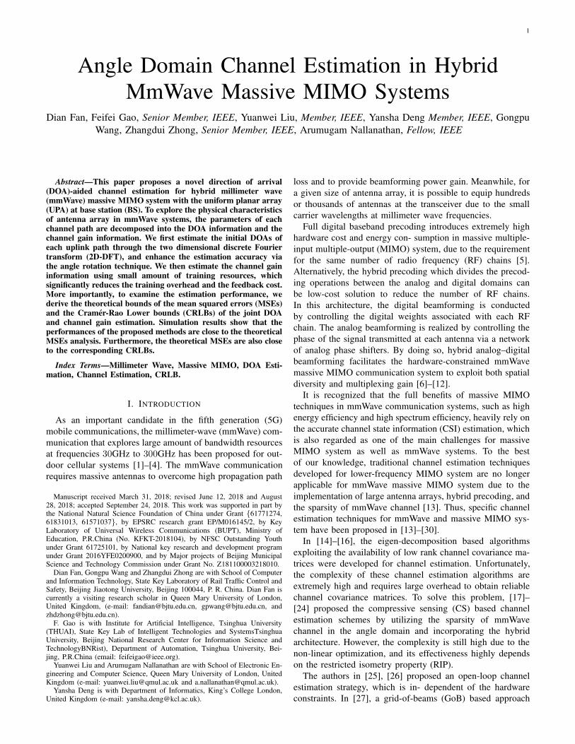
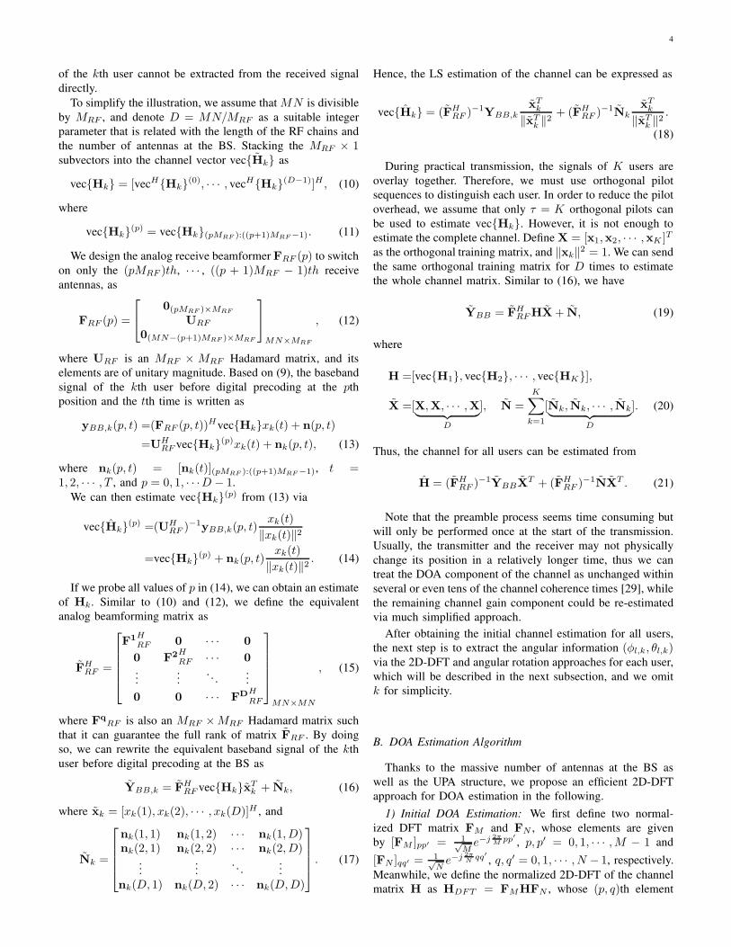
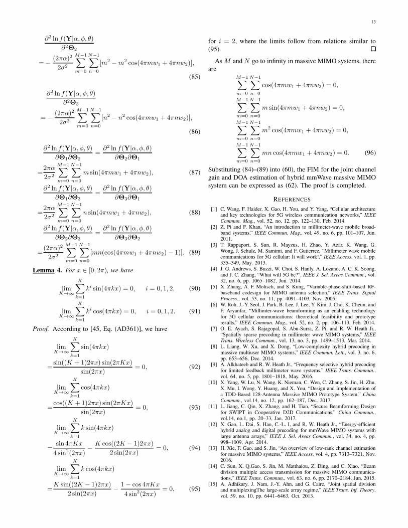
Fig. 1. Simplified system model of multiuser mmWave massive MIMO withhybrid precoding.

hybrid precoding and the channel characteristics are described.

In section III, we present a two-stage 2D-DFT aided DOA

estimation algorithm. The MSE and CRLB performance are

analyzed in the section IV. Simulation results are then provided

in Section V and conclusions are drawn in Section VI.

Notations: Small and upper bold-face letters donate column

vectors and matrices, respectively; the superscripts (·)H , (·)T ,

(·)∗, (·)−1, (·)† stand for the conjugate-transpose, transpose,

conjugate, inverse, pseudo-inverse of a matrix, respectively;

tr(A) donates the trace of A; [A]ij is the (i, j)th entry of A;

Diag{a} denotes a diagonal matrix with the diagonal element

constructed from a, while Diag{A} denotes a vector whose

elements are extracted from the diagonal components of A;

vec(A) denotes the vectorization of A; R{A} denotes the

real part of A; S{A} denotes the Imaginary part of A; [a]i:jdenotes the subvector of a that starts with [a]i and ends at [a]j ;

[A]i:j denotes the submatrix of A that starts with row [a]i,:and ends at row [a]j,:; E{·} denotes the statistical expectation,

and ‖h‖ is the Euclidean norm of h.

II. SYSTEM MODEL

Let us consider a multiuser mmWave massive MIMO time

division duplex (TDD) systems with a hybrid precoding struc-

ture as shown in Fig. 1. The BS is equipped with MNantennas in the form of UPA where M represents the number

of antennas in the horizon and N represents the number of

antennas in the vertical. The BS has MRF ≤ M×N RF chains

transmitting data streams to K ≤ MRF mobile users, each

with a single antenna [19]. We denote the distance between

the neighboring antenna elements in both horizon and vertical

as d. The BS is assumed to apply an MRF×K complex valued

based-band digital beamformer FBB(FBB ∈ CMRF×K), fol-

lowed by an analog beamformer FRF (FRF ∈ CMN×MRF ).To simplify the hardware implementation, each element of

FRF has unitary magnitude with arbitrary phase. As FRF

is implemented using analog phase shifters, its elements are

constrained to satisfy [[FRF ]:,j [FRF ]∗:,j ]i,i = 1

MN , (j =1, 2, · · ·MRF , i = 1, 2, · · ·MN), where all elements of FRF

have equal norm. The total transmit power constraint is en-

forced by normalizing FBB to satisfy ‖FRF [FBB]:,k‖2F = 1,

k = 1, 2, · · · ,K .

A. Transmitter Model

Denote Hk as the M ×N channel matrix between the BS

and the kth mobile user. In the uplink transmission stage, the

3

A(φl,k, θl,k) =1√MN

1 · · · ej2πd/λ(N−1) sinφl,k cos θl,k

.... . .

...

ej2πd/λ(M−1) cosφl,k · · · ej2πd/λ((M−1) cosφl,k+(N−1) sinφl,k cos θl,k)

M×N

, (4)

received signal at the BS can be expressed as

y(t) = FHBBF

HRF

K∑

k=1

vec{Hk}sk(t) +N, t = 1, · · · , T, (1)

where sk(t) is the transmitted signal at time t, N ∼CN (0, σ2

nI) is the complex Gaussian noise matrix, and σ2n

is the noise covariance.

Since the uplink and downlink channels are reciprocal in a

TDD system, the received signal in the downlink transmission

at the kth mobile user is given by

yk = vecH{Hk}FRFFBBs + nk, (2)

where s = [s1, s2, · · · , sK ]T is the transmitted signal vector

for all K mobile users. Thus, we can express the received

SNR at the kth mobile user as

Γk = |vecH{Hk}FRFFBB|2σ2s

σ2n

, (3)

where E{|sk|2} = σ2s denotes the power of sk.

B. Channel Model

Due to the limited scattering characteristics in the mmWave

environment [39]–[42], we assume the channel representa-

tion based on the extended Saleh-Valenzuela (SV) model

in [25]–[27]. Let us define φl,k ∈ [−90◦, 90◦) and θl,k ∈[−180◦, 180◦) as the signal elevation angle and the azimuth of

the lth (l = 1, 2, · · · , L) path of the kth user. The correspond-

ing steering matrix can be expressed as (4) shown on top of

this page, where λ is the wavelength of the carrier signal. De-

noting w1,l,k = 2πdλ cosφl,k and w2,l,k = 2πd

λ sinφl,k cos θl,k,

we can express (4) as

A(φl,k, θl,k) = A(w1,l,k, w2,l,k) = a(w1,l,k)aT (w2,l,k), (5)

where a(w1,l,k) = 1√M[1, · · · , ej(M−1)w1,l,k ]T , and

a(w2,l,k) =1√N[1, · · · , ej(N−1)w2,l,k ]T .

Using the geometric channel model with L scatters in

mmWave channel, where each scatter contributes to single

propagation path between the BS and the mobile user, we

can write the channel matrix as

Hk =1√L

L∑

l=1

al,kA(φl,k, θl,k)

=1√L

L∑

l=1

al,ka(w1,l,k)aT (w2,l,k)

=1√LAw1,kHa,kA

Tw2,k, (6)

where

Aw1,k = [a(w1,1,k), a(w1,2,k), · · · , a(w1,L,k)],

Aw2,k = [a(w2,1,k), a(w2,2,k), · · · , a(w2,L,k)],

Ha,k = diag(a1,k, a2,k, · · · , aL,k), (7)

and al,k is the channel gain along the lth path of the kth user

(l = 0 for the line-of-sight (LOS) path and l > 1 for the

non-line-of-sight (NLOS) paths).

The (m,n)th element of the channel matrix Hk can be

written as

[Hk]m,n =1√L

L∑

l=1

al,kej(mw1,l,k+nw2,l,k), (8)

with m = 0, 1, · · · ,M − 1, and n = 0, 1, · · · , N − 1. It is

worth noting that at mmWave frequencies, the amplitude of

channel gain |a1,k| of LOS components are typically 5 to 10dB

stronger than the {|al,k|}Ll=2 of the NLOS component [40].

Obviously, (6) is a sparse channel model that represents the

low rank property and the spatial correlation characteristics of

mmWave massive MIMO system. Importantly, the parameters

of Hk have only L complex channel gains and 2L real

phases (φl,k, θl,k), where the number of paths is usually much

less than the number of antennas, i.e., L ≪ MN . Instead

of directly estimating the channel Hk, one could first esti-

mate the DOA information (φl,k, θl,k), and then estimate the

corresponding path gain al,k via the conventional estimation

theory, such as least square (LS), maximum-likelihood (ML)

algorithms. By doing this, the number of the parameters to

be estimated is greatly reduced [43]. It is noted that the

beamspace method and CS method from channel model (6) is

not the real physical angle, but only provide an approximation

of the quantized angle with limited resolution.

III. DOA ESTIMATION FROM ARRAY SIGNAL PROCESSING

In this section, we propose a new DOA estimation algorithm

for the hybrid antenna array. To facilitate the understanding,

we start with the uplink transmission.

A. Preamble

In the uplink transmission, the preamble will only be sent

once at the beginning of the transmission. The received signal

at the BS can be written as

YBB = FHRF

K∑

k=1

vec{Hk}xTk +N, (9)

where xk = [xk,1, xk,2, · · · , xk,τ ]T is the preamble of the

kth user, τ ≥ K is the length of preamble, and YBB is the

baseband signal before the digital precoding in the BS. Since

the received signal has only a few observations, the whole CSI

4

of the kth user cannot be extracted from the received signal

directly.

To simplify the illustration, we assume that MN is divisible

by MRF , and denote D = MN/MRF as a suitable integer

parameter that is related with the length of the RF chains and

the number of antennas at the BS. Stacking the MRF × 1subvectors into the channel vector vec{Hk} as

vec{Hk} = [vecH{Hk}(0), · · · , vecH{Hk}(D−1)]H , (10)

where

vec{Hk}(p) = vec{Hk}(pMRF ):((p+1)MRF−1). (11)

We design the analog receive beamformer FRF (p) to switch

on only the (pMRF )th, · · · , ((p + 1)MRF − 1)th receive

antennas, as

FRF (p) =

0(pMRF )×MRF

URF

0(MN−(p+1)MRF )×MRF

MN×MRF

, (12)

where URF is an MRF × MRF Hadamard matrix, and its

elements are of unitary magnitude. Based on (9), the baseband

signal of the kth user before digital precoding at the pth

position and the tth time is written as

yBB,k(p, t) =(FRF (p, t))Hvec{Hk}xk(t) + n(p, t)

=UHRF vec{Hk}(p)xk(t) + nk(p, t), (13)

where nk(p, t) = [nk(t)](pMRF ):((p+1)MRF−1), t =1, 2, · · · , T , and p = 0, 1, · · ·D − 1.

We can then estimate vec{Hk}(p) from (13) via

vec{Hk}(p) =(UHRF )

−1yBB,k(p, t)xk(t)

‖xk(t)‖2

=vec{Hk}(p) + nk(p, t)xk(t)

‖xk(t)‖2. (14)

If we probe all values of p in (14), we can obtain an estimate

of Hk. Similar to (10) and (12), we define the equivalent

analog beamforming matrix as

FHRF =

F1HRF 0 · · · 0

0 F2HRF · · · 0

......

. . ....

0 0 · · · FDHRF

MN×MN

, (15)

where FqRF is also an MRF ×MRF Hadamard matrix such

that it can guarantee the full rank of matrix FRF . By doing

so, we can rewrite the equivalent baseband signal of the kth

user before digital precoding at the BS as

YBB,k = FHRF vec{Hk}xT

k + Nk, (16)

where xk = [xk(1), xk(2), · · · , xk(D)]H , and

Nk =

nk(1, 1) nk(1, 2) · · · nk(1, D)nk(2, 1) nk(2, 2) · · · nk(2, D)

......

. . ....

nk(D, 1) nk(D, 2) · · · nk(D,D)

. (17)

Hence, the LS estimation of the channel can be expressed as

vec{Hk} = (FHRF )

−1YBB,kxTk

‖xTk ‖2

+ (FHRF )

−1NkxTk

‖xTk ‖2

.

(18)

During practical transmission, the signals of K users are

overlay together. Therefore, we must use orthogonal pilot

sequences to distinguish each user. In order to reduce the pilot

overhead, we assume that only τ = K orthogonal pilots can

be used to estimate vec{Hk}. However, it is not enough to

estimate the complete channel. Define X = [x1,x2, · · · ,xK ]T

as the orthogonal training matrix, and ‖xk‖2 = 1. We can send

the same orthogonal training matrix for D times to estimate

the whole channel matrix. Similar to (16), we have

YBB = FHRFHX+ N, (19)

where

H =[vec{H1}, vec{H2}, · · · , vec{HK}],

X =[X,X, · · · ,X︸ ︷︷ ︸

D

], N =

K∑

k=1

[Nk, Nk, · · · , Nk︸ ︷︷ ︸

D

]. (20)

Thus, the channel for all users can be estimated from

H = (FHRF )

−1YBBXT + (FH

RF )−1NXT . (21)

Note that the preamble process seems time consuming but

will only be performed once at the start of the transmission.

Usually, the transmitter and the receiver may not physically

change its position in a relatively longer time, thus we can

treat the DOA component of the channel as unchanged within

several or even tens of the channel coherence times [29], while

the remaining channel gain component could be re-estimated

via much simplified approach.

After obtaining the initial channel estimation for all users,

the next step is to extract the angular information (φl,k, θl,k)via the 2D-DFT and angular rotation approaches for each user,

which will be described in the next subsection, and we omit

k for simplicity.

B. DOA Estimation Algorithm

Thanks to the massive number of antennas at the BS as

well as the UPA structure, we propose an efficient 2D-DFT

approach for DOA estimation in the following.

1) Initial DOA Estimation: We first define two normal-

ized DFT matrix FM and FN , whose elements are given

by [FM ]pp′ = 1√Me−j 2π

Mpp′

, p, p′ = 0, 1, · · · ,M − 1 and

[FN ]qq′ =1√Ne−j 2π

Nqq′ , q, q′ = 0, 1, · · · , N − 1, respectively.

Meanwhile, we define the normalized 2D-DFT of the channel

matrix H as HDFT = FMHFN , whose (p, q)th element

5

(p = 0, 1, ...,M − 1; q = 0, 1, ..., N − 1) is computed as

[HDFT ]pq =1√MN

M−1∑

m=0

N−1∑

n=0

[H]pqe−j2π( pm

M+ qn

N )

=1√

LMN

L∑

l=1

ale−j M−1

2( 2πM

p−w1,l)e−j N−1

2( 2π

Nq−w2,l)

×sin(

πp− Mw1,l

2

)

sin((πp− Mw1,l

2 )/M)·

sin(

πq − Nw2,l

2

)

sin((πq − Nw2,l

2 )/N). (22)

It is noted that with infinite number of antennas in the array,

i.e., M → ∞, N → ∞, there always exists some integers pl =Mw1,l

2π , ql =Nw2,l

2π such that [HDFT ]plql =al√

LMN, while the

other elements of HDFT are all zero, In other words, all power

is concentrated on the (pl, ql)th elements and the elements of

HDFT possess sparse property, such that the elevation and

the azimuth DOA of the lth path (φl, θl) can be immediately

estimated from the non-zero positions (pl, ql) of HDFT using

φl =cos−1

(λplMd

)

,

θl =cos−1

λqlNd

/√

1−(λplMd

)2

. (23)

Unfortunately, in practice, the array aperture cannot be

infinitely large, even if MN could be as greater as hun-

dreds or thousands in hybrid mmWave massive MIMO

systems. In special case, if some specific angles satisfy

that Mw1,l/(2π) is integer and Nw2,l/(2π) is integer, all

power of channel will concentrate on some separated sin-

gle points. We call these as on-grid angles. In more gen-

eral case, Mw1,l/(2π) and Nw2,l/(2π) will not be inte-

gers, and the channel power of HDFT will leak from the

(⌊Mw1,l/(2π)⌉, ⌊Nw2,l/(2π)⌉)th element to its nearby ele-

ments. In fact, the leakage of channel power is positively pro-

portional to the deviation (Mw1,l/(2π)−⌊Mw1,l/(2π)⌉) and

(Nw2,l/(2π) − ⌊Nw2,l/(2π)⌉), but is inversely proportional

to M and N as shown in (22). However, HDFT can still be

approximated as a sparse matrix with most of power concen-

trated around the (⌊Mw1,l/(2π)⌉, ⌊Nw2,l/(2π)⌉)th element.

Hence, the peak power position of HDFT is still useful for

extracting initial DOA information.

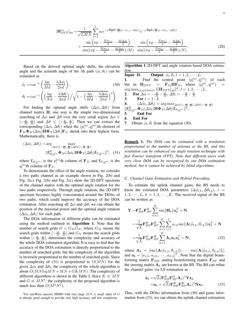
An example of a two-path channel from (30◦, 140◦) and

(−50◦, 10◦) with M = 100, N = 100 as shown in Fig. 2(a),

whose channel sparse characteristics after 2D-DFT is depicted.

For clear illustration, we demonstrate only for a noise-free

scenario. It can be seen that each path corresponds to one bin

and each bin has a central point that contains the largest power.

Each bin encounters the power leakage and the points around

the central point also contain considerable power but the power

of other points are ignorable. In Fig. 2(a), the central point of

the channel after initial 2D-DFT are (69, 65) and (41, 25).Hence, we can use these two peak power positions as the

initial DOA estimation.

Based on the above discussion, we can formulate the 2D-

DFT of the estimated channel matrix H, with its (p, q)th

Fig. 2. An example of a two paths channel sparse characteristics after 2D-DFT and optimal angle rotation, where BS array has 100× 100 antennas.

element being

[HDFT ]pq = [HDFT ]pq + [NDFT ]pq, (24)

where NDFT ∼ CN(

0,σ2

n√MN

I)

. Denote the L largest peaks

in L bins of HDFT as (pinil , qinil ). We can express the initial

DOA estimates as

φinil =cos−1

(λpinil

Md

)

,

θinil =cos−1

λqinil

Nd

/√

1−(λpinil

Md

)2

. (25)

2) Fine DOA Estimation: The resolution of (φinil , θinil )

via directly applying 2D-DFT is limited by half of the DFT

interval, i.e., 1/(2M) and 1/(2N). For example, for M = 100and N = 100, the worst MSE of the (φini

l , θinil ) is in the order

of 10−4. To improve the DOA estimation accuracy, we next

show how this mismatch could be compensated via an angle

rotation operation.

The angle rotation of the original channel matrix is defined

as

Hro = ΦM (∆φl)HΦN (∆θl), (26)

where the diagonal matrices ΦM (∆φl) and ΦN (∆θl) are

given by

ΦM (∆φl) = diag{1, ej∆φl , · · · , ej(M−1)∆φl},ΦN(∆θl) = diag{1, ej∆θl , · · · , ej(N−1)∆θl}. (27)

In (27), ∆φl ∈ [− πM , π

M ] and ∆θl ∈ [− πN , π

N ] are the angle

rotation parameters. After the angle rotation operation, the 2D-

DFT of the rotated channel matrix HroDFT can be calculated

as (28) shown on top of next page.

It can be readily found that the entries of HroDFT have only

L non-zero elements when the angle shifts satisfying

∆φl = 2πpl/M − w1,l, ∆θl = 2πql/N − w2,l, (29)

where (∆φl,∆θl) in (29) are the optimal angle shifts.

6

[HroDFT ]pq =

1√LMN

L∑

l=1

ale−j M−1

2( 2πM

p−w1,l−∆φl)e−j N−1

2( 2π

Nq−w2,l−∆θl)

×sin(

πp− Mw1,l

2 − M∆φl

2

)

sin((πp− Mw1,l

2 − M∆φl

2 )/M)·

sin(

πq − Nw2,l

2 − N∆θl2

)

sin((πq − Nw2,l

2 − N∆θl2 )/N)

. (28)

Based on the derived optimal angle shifts, the elevation

angle and the azimuth angle of the lth path (φl, θl) can be

estimated as

φl =cos−1

(λplMd

− λ∆φl

2πd

)

, (30)

θl =cos−1

((λqlNd

− λ∆θl2πd

)/√

1−( λplMd

− λ∆φl

2πd

)2)

.

For finding the optimal angle shifts (∆φl,∆θl) from

channel matrix H, one way is the simple two-dimensional

searching of ∆φ and ∆θ over the very small region ∆φ ∈[− π

M , πM ] and ∆θ ∈ [− π

N , πN ]. Then we can extract the

corresponding (∆φl,∆θl) when the (pinil , qinil )th element of

FMΦM (∆φl)HΦN (∆θl)FN shrink into their highest form.

Mathematically, there is

(∆φl,∆θl) = arg max∆φ∈[− π

M, πM

],∆θ∈[− πN

, πN

]

‖fHMpinil

ΦM (∆φl)HΦN (∆θl)fNqinil

‖2, (31)

where fMpinil

is the pinil th column of FM and fNqinil

is the

qinil th column of FN .

To demonstrate the effect of the angle rotation, we consider

a two paths channel as an example shown in Fig. 2(b) and

Fig. 2(c). Fig. 2(b) and Fig. 2(c) show the 2D-DFT spectrum

of the channel matrix with the optimal angle rotation for the

two paths respectively. Through angle rotation, the 2D-DFT

spectrum becomes highly concentrated around the DOAs of

two paths, which could improve the accuracy of the DOA

estimation. After searching all ∆φ and ∆θ, we can obtain the

position of the maximal power and the optimal angle rotation

(∆φl,∆θl) for each path.

The DOA information of different paths can be estimated

using the method outlined in Algorithm 1. Note that the

number of search grids G = GMGN , where GM means the

search grids within [− πM , π

M ] and GN means the search grids

within [− πN , π

N ], determines the complexity and accuracy of

the whole DOA estimation algorithm. It is easy to find that the

accuracy of the DOA estimation is directly proportional to the

number of searched grids, but the complexity of the algorithm

is inversely proportional to the number of searched grids. Since

the complexity of (31) is proportional to O(MN) for the

given ∆φl and ∆θl, the complexity of the whole algorithm is

about O(MNlogMN+MN +GKMN). The complexity of

different algorithms is shown in the Table I. Since K ≪ MNand G ≪ MN 1, the complexity of the proposed algorithm is

much less than O(M2N2).

1For mmWave massive MIMO with very large MN , a small value of Gis already good enough to provide very high accuracy and low complexity.

Algorithm 1 2D-DFT and angle rotation based DOA estima-

tion

Input: H. Output: φl, θl, l = 1, 2, · · · , L.

1. Find the central point (pinil , qinil ) of each

bin in HDFT = FMHFN , where (pinil , qinil ) =argmax(p,q)∈bin(l) ‖[HDFT ]pq‖2, l = 1, 2, · · · , L.

2. For ∆φ = − πM : π

M , ∆θl = − πN : π

N3. For l = 1 : L4. (∆φl,∆θl) = argmax∆φ∈[− π

M, πM

],∆θ∈[− πN

, πN

]

‖fHMpinil

ΦM (∆φl)HΦN (∆θl)fNqinil

‖2,

5. End For

6. End For

7. Obtain φl, θl from the equation (30).

Remark 1. The DOA can be estimated with a resolution

proportional to the number of antenna at the BS, and this

resolution can be enhanced via angle rotation technique with

fast Fourier transform (FFT). Note that different users with

very close DOA can be recognized by our DOA estimation

method, but it cannot be achieved by blind algorithms.

C. Channel Gain Estimation and Hybrid Precoding

To estimate the uplink channel gains, the BS needs to

know the estimated DOA parameters (∆φl,k,∆θl,k), l =1, 2, · · · , L, k = 1, 2, · · · ,K . The received signal of the BS

can be written as

Y =FHBBF

HRF

K∑

k=1

vec{Hk}xTk +N

=1√LFH

BBFHRF

K∑

k=1

L∑

l=1

al,kvec{A(φl,k, θl,k)}xTk +N

=1√LFH

BBFHRF

K∑

k=1

AkakxTk +N, (32)

where Ak = [vec{A(φ1,k, θ1,k)}, · · · , vec{A(φL,k, θL,k)}],and ak = [a1,k, a2,k, · · · , aL,k]

T . Note that the digital beam-

forming matrix FBB , analog beamforming matrix FRF and

the steering matrix Ak are known at the BS. The BS can refine

the channel gains via LS estimation as

ak =√L(FH

BBFHRFAk)

†Yxk

=ak +√L(FH

BBFHRFAk)

†Nxk. (33)

Thus, with the DOAs information from (30) and gains infor-

mation from (33), we can obtain the uplink channel estimation

7

TABLE ICOMPLEXITY OF DIFFERENT ESTIMATE ALGORITHMS

Algorithm Complexity

Proposed 2D-DFT and angle rotation estimate algorithm O(MNlogMN +MN +GKMN)Beamspace estimate algorithm O(MNlogMN +MN)

CS estimate algorithm O(M2N2 +KMN)

for all users as

Hk =1√L

L∑

l=1

al,kvec{A(φl,k, θl,k)}. (34)

From (2), the downlink received signals can be expressed

as

yd = HdFRFFBBs+ n, (35)

where Hd = [vec{H1}, vec{H2}, · · · , vec{HK}]H , and n ∼CN (0, σ2

nIK) is additive white Gaussian noise vector. We

assume MRF = KL. From the previous discussion, the analog

precoding matrix can be immediately obtained from

FRF = [vec{ΦM (∆φ1,1)fMp1,1fN

Hq1,1ΦN (∆θ1,1)}, · · · ,

vec{ΦM (∆φL,K)fMpL,KfN

HqL,K

ΦN (∆θL,K)}], (36)

where (pl,k, ql,k) denotes the position that contains the largest

power after 2D-DFT of the lth path of the kth user, and

each column of FRF represents the spatial angle (after angle

rotation) of each path for all K users. Note that the analog

precoding indicates that each path of each user is transmitting

exactly towards its signal direction and is thus named as

anglespace transmission2.

Similar to the conventional digital precoding approach,

FBB can be obtained via the zero-forcing (ZF) beamforming

algorithm, as

FBB =1√P(HdFRF )

H((HdFRF )(HdFRF )

H)−1, (37)

where P is the power constraint.

Remark 2. The reciprocity of the channel cannot be applied

to the frequency division duplex (FDD) system due to the

different transmission frequencies of the uplink and downlink

channels. Nonetheless, the uplink and downlink channels share

a common propagation space between the BS and the user. The

spatial directions or angles in the uplink channel are almost

the same as those in the downlink channel. For example,

the DOA information of both uplink and downlink are the

same. Therefore, our DOA estimation algorithm can also be

applied to FDD system and the channel gain component of

the downlink can be estimated using small training overhead.

IV. PERFORMANCE ANALYSIS

In this section, we derive the theoretical MSE of the joint

DOA and channel gain estimation for hybrid mmWave massive

MIMO system. Generally, a closed-form MSE analysis for

multiple DOA estimations is hard to obtain. An alternatively

acceptable approach is to consider single user and single

2This is a key difference from beamspace transmission.

propagation path and derive corresponding MSE of φ, θ as a

benchmark [44]. We first show that the MSE of the proposed

estimation algorithm is the same as the ML estimator in

single propagation path scenario and derive the closed-form

expressions of the DOA information and channel gain using

the ML estimator in the high SNR region. Next, the CRLB

analysis of the DOA information and channel gain are carried

on.

A. Theoretical MSE of The Proposed Estimator

Limiting to single propagation path, the received signal can

be rewritten as

y = FHRF vec(H)s+ n = FH

RF vec(A)αs+ n, (38)

where A , A(w1, w2) is the M ×N steering matrix with its

(p, q)th entry given by

[A]pq = ej((p−1)w1+(q−1)w2), (39)

and n is the MRF × 1 vector representing the white Gaussian

noise with zero mean and variance σ2n.

The proposed estimator can be rewritten as

[w1, w2] = argmaxw1,w2

‖vecH(A)(FHRF )

†y‖2

=argmaxw1,w2

yHFHRF vec(A)vecH(A)(FH

RF )†y, (40)

where vec(A) = vec{ΦM (∆φ)fMpfNHq ΦN (∆θ)}.

For given w1, w2 and α, the probability density function

(PDF) of y can be expressed as

f(y|w1, w2, α)

=1

(πσ2n)

MRFexp

{

−‖y− FHRF vec(A)αs‖2

σ2n

}

. (41)

The joint ML estimates of w1, w2 and α can be obtained via

[w1, w2, α] = argmaxw1,w2,α

f(y|w1, w2, α), (42)

or equivalently

[w1, w2, α] = argminw1,w2,α

‖y− FHRF vec(A)αs‖2. (43)

In the next analysis, we first estimate w1 and w2, and then

estimate channel gain a, which is a two-step optimization

rather than joint optimization.

For given w1 and w2, the ML estimate of α is obtained

from (43) as

α = vecH(A)(FHRF )

†s∗y. (44)

8

Substituting (44) into (43), the ML estimates of w1, w2 can

be written as

[w1, w2] = argminw1,w2

‖y − FHRF vec(A)vecH(A)(FH

RF )†s∗ys‖2

=argminw1,w2

‖y − σ2sF

HRF vec(A)vecH(A)(FH

RF )†y‖2

=argmaxw1,w2

yHFHRFPA(FH

RF )†y

=argmaxw1,w2

g(w1, w2), (45)

where g(w1, w2) denotes the cost function of w1, w2, s∗s =σ2s means the power of signal, and PA = vec(A)vecH(A)

represents the projection matrix onto the subspace spanned by

vec(A). Interestingly, the MSE (40) of the proposed estimator

coincides with the ML estimator (45). Till now, we have (44)

and (45) as the ML estimates of α, w1, and w2.

Lemma 1. Under high SNR, the perturbations of the estima-

tion of w1 and w2 from (45) are given by

E{∆w2i } =

σ2n

2σ2s |α|2vecH(A)WiP⊥

a Wivec(A), (46)

where i = 1, 2, P⊥a = I − Pa is the projection matrix onto

the orthogonal space spanned by A, and W1, W2 are the

diagonal matrices as

W1 = Diag{0. · · · , 0︸ ︷︷ ︸

N

, · · · , (M − 1), · · · , (M − 1)︸ ︷︷ ︸

N

}, (47)

W2 = Diag{0. · · · , 0︸ ︷︷ ︸

M

, · · · , (N − 1), · · · , (N − 1)︸ ︷︷ ︸

M

}. (48)

Proof. See Appendix.

In the channel estimation process, we need to further exam-

ine the MSE of the azimuth angle φ and the elevation angle θ.

Based on the fact that w1 = 2πdλ cosφ, w2 = 2πd

λ sinφ cos θ,

we have

φ = cos−1

(λw1

2πd

)

, and θ = cos−1

(λw2

2πd sinφ

)

. (49)

From (46) and (49), we can derive the mean and the MSE

of the azimuth angle and the elevation angle, namely

E{∆φ} = E{∆θ} = 0,

E{∆φ2} = E{(φ− φ)(φ − φ)H} =∂φ

∂w1E{w2

1}(∂φ

∂w1)H

=( λ2πd )

2

1− (λw1

2πd )2× σ2

n/σ2s

2|α|2vecH(A)W1P⊥a W1vec(A)

,

E{∆θ2} = E{(θ − θ)(θ − θ)H} =∂θ

∂w2E{w2

2}(∂θ

∂w2)H

=( λ2πd sinφ )

2

1− ( λw2

2πd sinφ )2× σ2

n/σ2s

2|α|2vecH(A)W2P⊥a W2vec(A)

.

(50)

Based on (44), we write α as

α =vecH(A)(FHRF )

†s∗(FHRF vec(A)αs∗ + n)

=σ2svecH(A)vec(A)α + vecH(A)(FH

RF )†s∗n, (51)

where vecH(A) is constructed from the estimate (w1, w2).With the help of Taylor’s expansion, vecH(A) can be approx-

imated by

vecH(A) ≈ vecH(A) + jvecH(A)Wi∆wi, i = 1, 2. (52)

Substituting (52) into (51), we rewrite α as

α =σ2s (vecH(A) + jvecH(A)W1∆w1)vec(A)α (53)

+ vecH(A)(FHRF )

†s∗n

=α+ jvecH(A)W1vec(A)∆w1α+ vecH(A)(FHRF )

†s∗n.

With the help of (46), we can derive the mean and the MSE

of the channel gain estimation as

E{∆α} =E{jvecH(A)W1vec(A)∆w1α

+ vecH(A)(FHRF )

†s∗n}

= 0,

E{∆α2} =E{(α− α)(α − α)H}=αE{(∆w1)

2}αH |vecH(A)W1vec(A)|2

+ σ2svecH(A)(FH

RF )†E{nnH}((FH

RF )†)Hvec(A)

=σ2n|vecH(A)W1vec(A)|2

2σ2svecH(A)W1P⊥

a W1vec(A)+ σ2

n. (54)

In (54), the first term is caused by the estimation error in (φ, θ),while the second part is caused by the noise only. If (φ, θ)are perfectly estimated, E{∆α2} only depends on the second

term in (54), which makes it equivalent to the covariance of

the traditional channel estimation methods.

Theorem 1. The MSE of α is then given by

MSE(α) =σ2n|vecH(A)W1vec(A)|2

2σ2svecH(A)W1P⊥

a W1vec(A)+ σ2

n. (55)

From (50) and (54), we know that the joint ML estimator

is unbiased for both (φ, θ) and α. Thus the analysis on

their CRLBs are necessary to show the effectiveness of these

estimators, which will be provided in the next subsection.

B. CRLB Analysis

In this subsection, we compute the CRLBs for the channel

gain and the DOA estimation under UPA antenna configu-

rations. It is worth noting that the MSE of the proposed

estimators is irrelevant to analog beamforming. Thus, we omit

analog beamforming for simplicity. With single LOS path

(L = 1), the received signal Y can be expressed as

Y =Hs+N = αA(φ, θ)s +N

=αa(w1)aT (w2)s+N. (56)

The (m,n)th received signal is given by

ym,n = αej((m−1)w1+(n−1)w2)s+ nm,n, (57)

where the real part of the received signal is

yRm,n =ℜ{ym,n} = ℜ{αej((m−1)w1+(n−1)w2)s}+ ℜ{nm,n}=xm,n + n′

m,n, (58)

9

I(Θ) =1

2σ2

MN 0 0

0 (2πα)2N∑M−1

m=0 m2 (2πα)2∑M−1

m=0 m∑N−1

n=0 n

0 (2πα)2∑M−1

m=0 m∑N−1

n=0 n (2πα)2M∑N−1

n=0 n2

. (62)

var(α) ≥A,

var(w1) ≥2σ2M

∑N−1n=0 n2

(2πα)2[N∑M−1

m=0 m2][M∑N−1

n=0 n2]− (2πα)2[∑M−1

m=0 m∑N−1

n=0 n][∑M−1

m=0 m∑N−1

n=0 n]= AB

6(2N − 1)

M − 1,

var(w2) ≥2σ2N

∑M−1m=0 m2

(2πα)2[N∑M−1

m=0 m2][M∑N−1

n=0 n2]− (2πα)2[∑M−1

m=0 m∑N−1

n=0 n][∑M−1

m=0 m∑N−1

n=0 n]= AB

6(2M − 1)

N − 1, (63)

xm,n = ℜ{αej((m−1)w1+(n−1)w2)s}, and n′m,n = ℜ{nm,n}.

For given α, φ, and θ, the probability density function of Y

can be expressed as

f(Y|α, φ, θ) = 1

(2πσ2)MN2

exp{−‖Y− αA(φ, θ)s‖2σ2

}

=1

(2πσ2)MN2

exp{− 1

2σ2

M∑

m=1

N∑

n=1

(yRm,n − xm,n)2}. (59)

Let us define Θ = [α,w1, w2]T as the unknown parameter

vector. The Fisher information matrix (FIM) is defined as

[I(Θ)]i,j = −E

[∂2 ln f(Y|α, φ, θ)

∂Θi∂Θj

]

, (60)

where

ln f(Y|α, φ, θ) = −MN

2ln(2πσ2)− 1

2σ2

M∑

m=1

N∑

n=1

n′2m,n,

(61)

and σ2 = σ2n/σ

2s .

Lemma 2. The FIM for the joint channel gain and DOA

estimation of hybrid mmWave massive MIMO systems can be

expressed as (62) shown on top of this page.

Proof. See Appendix.

Accordingly, the CRLB for the parameters of channel

gain and DOA are CRLB = I−1(Θ). Thus we have (63)

shown on top of this page, where A = 2σ2

MN , and B =1

(πα)2(7MN+M+N−5) .

Lemma 3. The CRLB of the azimuth and elevation angle can

be expressed as

var(θ) ≥ AB6(2N − 1)λ2

(M − 1)d2 sin2 θ, (64)

var(φ) ≥ AB6λ2(M − 1)(2M − 1) + 6(N − 1)Cd cos θ cosφ

(M − 1)(N − 1)d2 sin2 θ sin2 φ,

where C = 3λ(M − 1) + (2N − 1)d cos θ cosφ.

Proof. For DOA estimation of hybrid mmWave massive

MIMO system, the performance of azimuth angle θ and

elevation angle φ are required. Therefore, we can use the

following transformation to estimate the real angles of azimuth

and elevation:

g(Θ) =

αθφ

=

α

arccos(λw1

d )

arcsin( λw2

d sin θ )

. (65)

Then, we can obtain the CRLBs of the azimuth and eleva-

tion angle of hybrid mmWave massive MIMO system through

the following Jacobian matrix:

var(θ) ≥ [∂g(Θ)

∂ΘI−1(Θ)

∂g(ΘT )

∂Θ]2,2,

var(φ) ≥ [∂g(Θ)

∂ΘI−1(Θ)

∂g(ΘT )

∂Θ]3,3. (66)

Next, the CRLBs of the azimuth and elevation angle can be

expressed as

var(θ) ≥ AB6(2N − 1)λ2

(M − 1)d2 sin2 θ,

var(φ) ≥ 6ABλ2(M − 1)(2M − 1) + Cd cos θ cosφ

(M − 1)(N − 1)d2 sin2 θ sin2 φ, (67)

where C = 3λ(M−1)(N−1)+(N−1)(2N−1)d cos θ cosφ.

It is observed from (67) that the MSEs for both angle

and channel gain estimators are inversely proportional to the

SNR of the received signal, and the CRLBs decreases with

increasing the number of antenna array.

V. SIMULATION RESULTS

In this section, we show the effectiveness of the proposed

estimation method through numerical examples. In our simu-

lation, we consider a TDD mmWave massive MIMO system,

where the UPA at the BS has M = 100, N = 100 antennas

of d = λ/2, with MRF = 100 RF chains. There are

K = 10 single-antenna users uniformly distributed, and each

user has L = 10 paths. The default value of preamble τis set to be τ = 10. We use the ray-tracing way to model

the mmWave channels, and the channel matrix of different

users are formulated according to (6). We take angle rotation

search grids G = GMGN = 30× 30 = 900 unless otherwise

mentioned. In all examples, the DOA information of all users

are estimated from the preamble. With τ = 10, the overall

10

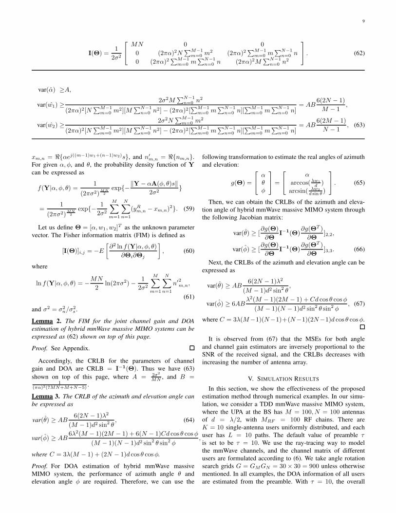
Fig. 3. Comparison of MSEs of the theoretical bound, CRLB, initialestimation method and the proposed DOA estimation schemes with searchingguides G = 10× 10, 20 × 20, 30 × 30, respectively.

users can transmit pilot synchronously such that the orthogonal

training can be applied to obtain the DOA information.

Fig. 3 plots the MSEs of DOA estimation as a function

of SNR for initial 2D-DFT, our proposed estimation method,

theoretical bound, and CRLB. The total transmission power for

uplink training is constrained to ρ for all users. It can be seen

that our proposed DOA estimation method performs slightly

worse than that of theoretical bound, but performs much better

than the initial estimation (2D-DFT) method. Interestingly,

the MSE of proposed DOA estimation method improves with

increasing the searching grid, which is due to the improved

angle resolution. If the searching grid goes to infinity, the

proposed DOA estimation method can achieve the same MSE

as the theoretical bound. It can also be seen from Fig. 3 that

the traditional initial estimation method remains constant for

any SNRs. The reason is that the Gaussian noise will keep the

same level after the 2D-DFT, such that the power of noise will

keep constant in all SNRs. In addition, the theoretical MSE is

very close to the corresponding CRLB.

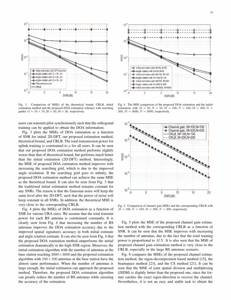
Fig. 4 plots the MSEs of DOA estimation as a function of

SNR for various URA sizes. We assume that the total transmit

power for each BS antenna is constrained constantly. It is

clearly seen from Fig. 4 that increasing the number of BS

antennas improves the DOA estimation accuracy due to the

improved spatial signatures accuracy in both initial estimate

and angle rotation estimate. It can also be seen from Fig. 4 that

the proposed DOA estimation method outperforms the initial

estimation dramatically in the high SNR region. Moreover, the

initial estimation algorithm with the number of antennas at the

base station reaching 3000×3000 and the proposed estimation

algorithm with 100×100 antennas at the base station have the

almost same performance. When the number of antennas is

large enough, the initial estimation can approach the proposed

method. Therefore, the proposed DOA estimation algorithm

can greatly reduce the number of BS antennas while ensuring

the accuracy of the estimation.

Fig. 4. The MSE comparison of the proposed DOA estimation and the initialestimation, with M = 50, N = 50,M = 100, N = 100,M = 200, N =200,M = 3000, N = 3000, respectively.

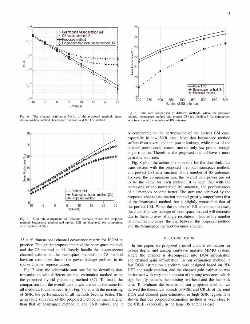
Fig. 5. Comparison of channel gain MSEs and the corresponding CRLB withM = 100, N = 100,M = 200, N = 200, respectively.

Fig. 5 plots the MSE of the proposed channel gain estima-

tion method with the corresponding CRLB as a function of

SNR. It can be seen that the MSE improves with increasing

the number of antennas, due to the fact that the total training

power is proportional to MN . It is also seen that the MSE of

proposed channel gain estimation method is very close to the

CRLB, especially in the large BS antennas scenario.

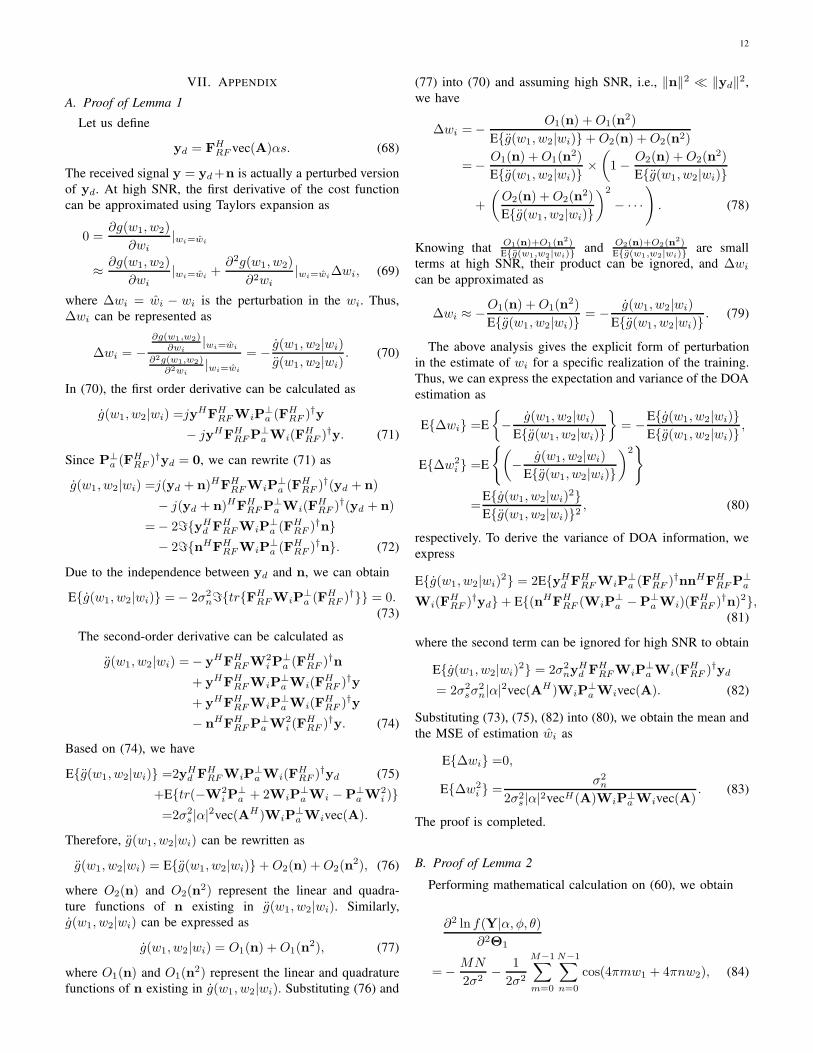
Fig. 6 compares the MSEs of the proposed channel estima-

tion method, the eigen-decomposition based method [15], the

beamspace method [23], and the CS method [21]. It can be

seen that the MSE of joint spatial division and multiplexing

(JSDM) is slightly better than the proposed one, since the for-

mer catches the exact eigen-direction to recover the channel.

Nevertheless, it is not an easy and stable task to obtain the

11

Fig. 6. The channel estimation MSEs of the proposed method, eigen-decomposition method, beamspace method, and the CS method.

Fig. 7. Sum rate comparison of different methods, where the proposedmethod, beamspace method and prefect CSI are displayed for comparisonas a function of SNR.

M ×N dimensional channel covariance matrix for JSDM in

practice. Though the proposed method, the beamspace method,

and the CS method could directly handle the instantaneous

channel estimation, the beamspace method and CS method

have an error floor due to the power leakage problem in its

sparse channel representation.

Fig. 7 plots the achievable sum rate for the downlink data

transmission with different channel estimation method using

the proposed hybrid precoding method (37). To make the

comparison fair, the overall data power are set as the same for

all methods. It can be seen from Fig. 7 that with the increasing

of SNR, the performances of all methods become better. The

achievable sum rate of the proposed method is much higher

than that of beamspace method in any SNR values, and it

Fig. 8. Sum rate comparison of different methods, where the proposedmethod, beamspace method and prefect CSI are displayed for comparisonas a function of the number of BS antennas.

is comparable to the performance of the prefect CSI case,

especially in low SNR case. Note that beamspace method

suffers from severe channel power leakage, while most of the

channel power could concentrate on only few points through

angle rotation. Therefore, the proposed method have a more

desirable sum rate.

Fig. 8 plots the achievable sum rate for the downlink data

transmission with the proposed method, beamspace method,

and prefect CSI as a function of the number of BS antennas.

To keep the comparison fair, the overall data power are set

to be the same for each method. It is seen that with the

increasing of the number of BS antennas, the performances

of all methods become better. The sum rate achieved by the

proposed channel estimation method greatly outperforms that

of the beamspace method, but is slightly worse than that of

the perfect CSI. When the number of BS antennas increases,

the channel power leakage of beamspace method will decrease

due to the improves of angle resolution. Thus as the number

of antennas increases, the gap between the proposed method

and the beamspace method becomes smaller.

VI. CONCLUSION

In this paper, we proposed a novel channel estimation for

hybrid digital and analog mmWave massive MIMO system,

where the channel is decomposed into DOA information

and channel gain information. In our estimation method, a

fast DOA estimation algorithm was designed based on 2D-

DFT and angle rotation, and the channel gain estimation was

performed with very small amount of training resources, which

significantly reduces the training overhead and the feedback

cost. To evaluate the benefits of our proposed method, we

derived the theoretical bounds of MSE and CRLB of the joint

DOA and channel gain estimation in high SNR region. It is

shown that our proposed estimation method is very close to

the CRLB, especially in the large BS antennas case.

12

VII. APPENDIX

A. Proof of Lemma 1

Let us define

yd = FHRF vec(A)αs. (68)

The received signal y = yd+n is actually a perturbed version

of yd. At high SNR, the first derivative of the cost function

can be approximated using Taylors expansion as

0 =∂g(w1, w2)

∂wi|wi=wi

≈ ∂g(w1, w2)

∂wi|wi=wi

+∂2g(w1, w2)

∂2wi|wi=wi

∆wi, (69)

where ∆wi = wi − wi is the perturbation in the wi. Thus,

∆wi can be represented as

∆wi = −∂g(w1,w2)

∂wi|wi=wi

∂2g(w1,w2)∂2wi

|wi=wi

= − g(w1, w2|wi)

g(w1, w2|wi). (70)

In (70), the first order derivative can be calculated as

g(w1, w2|wi) =jyHFHRFWiP

⊥a (F

HRF )

†y

− jyHFHRFP

⊥a Wi(F

HRF )

†y. (71)

Since P⊥a (F

HRF )

†yd = 0, we can rewrite (71) as

g(w1, w2|wi) =j(yd + n)HFHRFWiP

⊥a (F

HRF )

†(yd + n)

− j(yd + n)HFHRFP

⊥a Wi(F

HRF )

†(yd + n)

=− 2ℑ{yHd FH

RFWiP⊥a (F

HRF )

†n}− 2ℑ{nHFH

RFWiP⊥a (F

HRF )

†n}. (72)

Due to the independence between yd and n, we can obtain

E{g(w1, w2|wi)} =− 2σ2nℑ{tr{FH

RFWiP⊥a (F

HRF )

†}} = 0.(73)

The second-order derivative can be calculated as

g(w1, w2|wi) =− yHFHRFW

2iP

⊥a (F

HRF )

†n

+ yHFHRFWiP

⊥a Wi(F

HRF )

†y

+ yHFHRFWiP

⊥a Wi(F

HRF )

†y

− nHFHRFP

⊥a W

2i (F

HRF )

†y. (74)

Based on (74), we have

E{g(w1, w2|wi)} =2yHd FH

RFWiP⊥a Wi(F

HRF )

†yd (75)

+E{tr(−W2iP

⊥a + 2WiP

⊥a Wi −P⊥

a W2i )}

=2σ2s |α|2vec(AH)WiP

⊥a Wivec(A).

Therefore, g(w1, w2|wi) can be rewritten as

g(w1, w2|wi) = E{g(w1, w2|wi)}+O2(n) +O2(n2), (76)

where O2(n) and O2(n2) represent the linear and quadra-

ture functions of n existing in g(w1, w2|wi). Similarly,

g(w1, w2|wi) can be expressed as

g(w1, w2|wi) = O1(n) +O1(n2), (77)

where O1(n) and O1(n2) represent the linear and quadrature

functions of n existing in g(w1, w2|wi). Substituting (76) and

(77) into (70) and assuming high SNR, i.e., ‖n‖2 ≪ ‖yd‖2,

we have

∆wi =− O1(n) +O1(n2)

E{g(w1, w2|wi)}+O2(n) +O2(n2)

=− O1(n) +O1(n2)

E{g(w1, w2|wi)}×(

1− O2(n) +O2(n2)

E{g(w1, w2|wi)}

+

(O2(n) +O2(n

2)

E{g(w1, w2|wi)}

)2

− · · ·)

. (78)

Knowing thatO1(n)+O1(n

2)E{g(w1,w2|wi)} and

O2(n)+O2(n2)

E{g(w1,w2|wi)} are small

terms at high SNR, their product can be ignored, and ∆wi

can be approximated as

∆wi ≈ −O1(n) +O1(n2)

E{g(w1, w2|wi)}= − g(w1, w2|wi)

E{g(w1, w2|wi)}. (79)

The above analysis gives the explicit form of perturbation

in the estimate of wi for a specific realization of the training.

Thus, we can express the expectation and variance of the DOA

estimation as

E{∆wi} =E

{

− g(w1, w2|wi)

E{g(w1, w2|wi)}

}

= −E{g(w1, w2|wi)}E{g(w1, w2|wi)}

,

E{∆w2i } =E

{(

− g(w1, w2|wi)

E{g(w1, w2|wi)}

)2}

=E{g(w1, w2|wi)

2}E{g(w1, w2|wi)}2

, (80)

respectively. To derive the variance of DOA information, we

express

E{g(w1, w2|wi)2} = 2E{yH

d FHRFWiP

⊥a (F

HRF )

†nnHFHRFP

⊥a

Wi(FHRF )

†yd}+ E{(nHFHRF (WiP

⊥a −P⊥

a Wi)(FHRF )

†n)2},(81)

where the second term can be ignored for high SNR to obtain

E{g(w1, w2|wi)2} = 2σ2

nyHd FH

RFWiP⊥a Wi(F

HRF )

†yd

= 2σ2sσ

2n|α|2vec(AH)WiP

⊥a Wivec(A). (82)

Substituting (73), (75), (82) into (80), we obtain the mean and

the MSE of estimation wi as

E{∆wi} =0,

E{∆w2i } =

σ2n

2σ2s |α|2vecH(A)WiP⊥

a Wivec(A). (83)

The proof is completed.

B. Proof of Lemma 2

Performing mathematical calculation on (60), we obtain

∂2 ln f(Y|α, φ, θ)∂2Θ1

=− MN

2σ2− 1

2σ2

M−1∑

m=0

N−1∑

n=0

cos(4πmw1 + 4πnw2), (84)

13

∂2 ln f(Y|α, φ, θ)∂2Θ2

=− (2πα)2

2σ2

M−1∑

m=0

N−1∑

n=0

[m2 −m2 cos(4πmw1 + 4πnw2)],

(85)

∂2 ln f(Y|α, φ, θ)∂2Θ3

=− (2πα)2

2σ2

M−1∑

m=0

N−1∑

n=0

[n2 − n2 cos(4πmw1 + 4πnw2)],

(86)

∂2 ln f(Y|α, φ, θ)∂Θ1∂Θ2

=∂2 ln f(Y|α, φ, θ)

∂Θ2∂Θ1

=2πα

2σ2

M−1∑

m=0

N−1∑

n=0

m sin(4πmw1 + 4πnw2), (87)

∂2 ln f(Y|α, φ, θ)∂Θ1∂Θ3

=∂2 ln f(Y|α, φ, θ)

∂Θ3∂Θ1

=2πα

2σ2

M−1∑

m=0

N−1∑

n=0

n sin(4πmw1 + 4πnw2), (88)

∂2 ln f(Y|α, φ, θ)∂Θ2∂Θ3

=∂2 ln f(Y|α, φ, θ)

∂Θ3∂Θ2

=(2πα)2

2σ2

M−1∑

m=0

N−1∑

n=0

[mn(cos(4πmw1 + 4πnw2)− 1)]. (89)

Lemma 4. For x ∈ [0, 2π), we have

limK→∞

K∑

k=1

ki sin(4πkx) = 0, i = 0, 1, 2, (90)

limK→∞

K∑

k=1

ki cos(4πkx) = 0, i = 0, 1, 2. (91)

Proof. According to [45, Eq. (AD361)], we have

limK→∞

K∑

k=1

sin(4πkx)

=sin((K + 1)2πx) sin(2πKx)

sin(2πx)= 0, (92)

limK→∞

K∑

k=1

cos(4πkx)

=cos((K + 1)2πx) sin(2πKx)

sin(2πx)= 0, (93)

limK→∞

K∑

k=1

k sin(4πkx)

=sin 4πKx

4 sin2(2πx)− K cos((2K − 1)2πx)

2 sin(2πx)= 0, (94)

limK→∞

K∑

k=1

k cos(4πkx)

=K sin((2K − 1)2πx)

2 sin(2πx)− 1− cos 4πKx

4 sin2(2πx)= 0, (95)

for i = 2, where the limits follow from relations similar to

(95).

As M and N go to infinity in massive MIMO systems, there

are

M−1∑

m=0

N−1∑

n=0

cos(4πmw1 + 4πnw2) = 0,

M−1∑

m=0

N−1∑

n=0

m sin(4πmw1 + 4πnw2) = 0,

M−1∑

m=0

N−1∑

n=0

m2 cos(4πmw1 + 4πnw2) = 0,

M−1∑

m=0

N−1∑

n=0

mn cos(4πmw1 + 4πnw2) = 0. (96)

Substituting (84)–(89) into (60), the FIM for the joint channel

gain and DOA estimation of hybrid mmWave massive MIMO

system can be expressed as (62). The proof is completed.

REFERENCES

[1] C. Wang, F. Haider, X. Gao, H. You, and Y. Yang, “Cellular architectureand key technologies for 5G wireless communication networks,” IEEE

Commun. Mag., vol. 52, no. 12, pp. 122–130, Feb. 2014.[2] Z. Pi and F. Khan, “An introduction to millimeter-wave mobile broad-

band systems,” IEEE Commun. Mag., vol. 49, no. 6, pp. 101–107, Jun.2011.

[3] T. Rappaport, S. Sun, R. Mayzus, H. Zhao, Y. Azar, K. Wang, G.Wong, J. Schulz, M. Samimi, and F. Gutierrez, “Millimeter wave mobilecommunications for 5G cellular: It will work!,” IEEE Access, vol. 1, pp.335–349, May. 2013.

[4] J. G. Andrews, S. Buzzi, W. Choi, S. Hanly, A. Lozano, A. C. K. Soong,and J. C. Zhang, “What will 5G be?”, IEEE J. Sel. Areas Commun., vol.32, no. 6, pp. 1065–1082, Jun. 2014.

[5] X. Zhang, A. F. Molisch, and S. Kung, “Variable-phase-shift-based RF-baseband codesign for MIMO antenna selection,” IEEE Trans. SignalProcess., vol. 53, no. 11, pp. 4091–4103, Nov. 2005.

[6] W. Roh, J.-Y. Seol, J. Park, B. Lee, J. Lee, Y. Kim, J. Cho, K. Cheun, andF. Aryanfar, “Millimter-wave beamforming as an enabling technologyfor 5G cellular communications: theoretical feasibility and prototyperesults,” IEEE Commun. Mag., vol. 52, no. 2, pp. 106–113, Feb. 2014.

[7] O. E. Ayach, S. Rajagopal, S. Abu-Surra, Z. Pi, and R. W. Heath Jr.,“Spatially sparse precoding in millimeter wave MIMO systems,” IEEETrans. Wireless Commun., vol. 13, no. 3, pp. 1499–1513, Mar. 2014.

[8] L. Liang, W. Xu, and X. Dong, “Low-complexity hybrid precoding inmassive multiuser MIMO systems,” IEEE Commun. Lett., vol. 3, no. 6,pp. 653–656, Dec. 2014.

[9] A. Alkhateeb and R. W. Heath Jr., “Frequency selective hybrid precodingfor limited feedback millimeter wave systems,” IEEE Trans. Commun.,vol. 64, no. 5, pp. 1801–1818, May. 2016.

[10] X. Yang, W. Lu, N. Wang, K. Nieman, C. Wen, C. Zhang, S. Jin, H. Zhu,X. Mu, I. Wong, Y. Huang, and X. You, “Design and Implementation ofa TDD-Based 128-Antenna Massive MIMO Prototype System,” China

Commun., vol.14, no. 12, pp. 162–187, Dec. 2017.[11] L. Jiang, C. Qin, X. Zhang, and H. Tian, “Secure Beamforming Design

for SWIPT in Cooperative D2D Communications,” China Commun.,vol.14, no.1, pp. 20–33, Jan. 2017.

[12] X. Gao, L. Dai, S. Han, C.-L. I, and R. W. Heath Jr., “Energy-efficienthybrid analog and digital precoding for mmWave MIMO systems withlarge antenna arrays,” IEEE J. Sel. Areas Commun., vol. 34, no. 4, pp.998–1009, Apr. 2014.

[13] H. Xie, F. Gao, and S. Jin, “An overview of low-rank channel estimationfor massive MIMO systems,” IEEE Access, vol. 4, pp. 7313–7321, Nov.2016.

[14] C. Sun, X. Q.Gao, S. Jin, M. Matthaiou, Z. Ding, and C. Xiao, “Beamdivision multiple access transmission for massive MIMO communica-tions,” IEEE Trans. Commun., vol. 63, no. 6, pp. 2170–2184, Jun. 2015.

[15] A. Adhikary, J. Nam, J.-Y. Ahn, and G. Caire, “Joint spatial divisionand multiplexingThe large-scale array regime,” IEEE Trans. Inf. Theory,vol. 59, no. 10, pp. 6441–6463, Oct. 2013.

14

[16] H. Yin, D. Gesbert, M. Filippou, and Y. Liu, “A coordinated approachto channel estimation in large-scale multiple-antenna systems,” IEEE J.

Sel. Areas Commun., vol. 31, no. 2, pp. 264–273, Feb. 2013.

[17] S. L. H. Nguyen and A. Ghrayeb, “Compressive sensing-based channelestimation for massive multiuser MIMO systems,” in Proc. IEEE WCNC,Shanghai, China, Apr. 2013, pp. 2890–2895.

[18] X. Rao and V. K.Lau, “Distributed compressive CSIT estimation andfeed-back for FDD multi-user massive MIMO systems,” IEEE Trans.Signal Process., vol. 62, no. 12, pp. 3261–3271, Jun. 2014.

[19] A. Alkhateeb, O. E. Ayach, G. Leus, and R. W. Heath Jr., “Channelestimation and hybrid precoding for millimeter wave cellular systems,”IEEE J. Sel. Top. Signal Process., vol. 8, no. 5, pp. 831–846, Oct. 2014.

[20] A. Alkhateeb, G. Leus, and R. W. Heath, Jr., “Compressed sensingbased multi-user millimeter wave systems: How many measurementsare needed?” in Proc. IEEE Int. Conf. Acoust., Speech Signal Process.(ICASSP), Apr. 2015, pp. 2909–2913.

[21] Z. Gao, L. Dai, Z. Wang, and S. Chen, “Spatially common sparsity basedadaptive channel estimation and feedback for FDD massive MIMO,”IEEE Trans. Signal Process., vol. 63, no. 23, pp. 6169–6183, Dec. 2015.

[22] W. U. Bajwa, J. Haupt, A. M. Sayeed, and R. Nowak, “Compressedchannel sensing: A new approach to estimating sparse multipath chan-nels,” Proc. IEEE, vol. 98, no. 6, pp. 1058–1076, Jun. 2010.

[23] X. Gao, L. Dai, S. Han, C. I, X. Wang, “Reliable beamspace channelestimation for millimeter-wave massive MIMO systems with lens an-tenna array,” IEEE Wireless Commun., vol. 16, no. 9, pp. 6010–6021,Sep. 2017.

[24] C. Rusu, R. Mendez-Rial, N. Gonzalez-Prelcicy, and R. W. Heath Jr.,“Low complexity hybrid sparse precoding and combining in millimeterwave MIMO systems,” in Intern. Conf. Commun. (ICC’15). IEEE, Jun.2015, pp. 1340–1345.

[25] R. Mendez-Rial, C. Rusu, A. Alkhateeb, N. Gonzalez-Prelcicy, and R.W. Heath Jr., “Channel estimation and hybrid combining for mmWave:phase shifters or switches?,” in Proc. Inf. Theory Appl. Workshop, Feb.2015, pp. 90–97.

[26] R. Mendez-Rial, C. Rusu, N. Gonzalez-Prelcicy, A. Alkhateeb, andR. W. Heath Jr., “Hybrid MIMO architectures for millimeter wavecommunications: phase shifters or switches?,” IEEE Access, vol. 4, pp.247–267, Jan 2016.

[27] J. Singh and S. Ramakrishna, “On the feasibility of codebook-basedbeamforming in millimeter wave systems with multiple antenna arrays,”IEEE Trans. Wireless Commun., vol. 14, no. 5, pp. 2670–2683, May2015.

[28] R. Mendez-Rial, N. Gonzalez-Prelcicy, and R. W. Heath Jr., “Adaptivehybrid precoding and combining in mmWave multiuser MIMO systemsbased on compressed covariance estimation,” in Proc. Intern. Workshop

on Computational Advances in Multi-Sensor Adaptive Process., Dec.2015, pp. 213–216.

[29] H. Xie, F. Gao, S. Zhang, and S. Jin, “A unified transmission strategy forTDD/FDD massive MIMO systems with spatial basis expansion model,”IEEE Trans. Veh. Technol., vol. 66, no. 4, pp. 3170–3184, Apr. 2017.

[30] H. Xie, B. Wang, F. Gao, and S. Jin, “A full-space spectrum-sharingstrategy for massive MIMO cognitive radio systems,” IEEE J. Sel. Areas

Commun., vol. 34, no. 10, pp. 2537–2549, Oct. 2016.

[31] R. O. Schmidt, “Multiple emitter location and signal parameter estima-tion,” IEEE Trans. Antennas Propag., vol. 34, no. 3, pp. 276–280, Mar.1986.

[32] R. Roy and T. Kailath, “Esprit-estimation of signal parameters viarotational invariance techniques,” IEEE Trans. Acoust., Speech, Signal

Process., vol. 37, no. 7, pp. 984–995, Jul. 1989.

[33] H. Krim and M. Viberg, “Two decades of array signal processingresearch: the parametric approach,” IEEE Signal Process. Mag., vol.13, no. 4, pp. 67–94, Jul. 1996.

[34] T. Wang, B. Ai, R. He, and Z. Zhong, “Two-dimension direction-of-arrival estimation for massive MIMO systems,” IEEE Access, vol. 3,pp. 2122–2128, Nov. 2015.

[35] A. Hu, T. Lv, H. Gao, Z. Zhang, and S. Yang, “An ESPRIT-basedapproach for 2-D localization of incoherently distributed sources inmassive MIMO systems,” IEEE J. Sel. Topics Signal Process., vol. 8,no. 5, pp. 996–1011, Oct. 2014.

[36] A. Wang, L. Liu, and J. Zhang, “Low complexity direction of arrival(DOA) estiamtion for 2D massive MIMO systems,” in Proc. Global

Telecomm. Conf., Dec. 2012, pp. 703–707.

[37] L. Cheng, Y.-C. Wu, J. Zhang, and L. Liu, “Subspace identificationfor DOA estimation in massive/full-dimension MIMO systems: baddata mitigation and automatic source enumeration,” IEEE Trans. Signal

Process., vol. 63, no. 22, pp. 5897–5909, Nov. 2015.

[38] R. Shafin, L. Liu, and J. Zhang, “DoA estimation and capacity analysisfor 3D massive-MIMO/FD-MIMO OFDM system,” in Proc. Global

Conf. on Signal and Information Process., Dec. 2015, pp. 181–184.[39] T. Rappaport, Y. Qiao, J. Tamir, J. Murdock, and E. Ben-Dor, “Cellular

broadband millimeter wave propagation and angle of arrival for adaptivebeam steering systems,” in Proc. Radio and Wireless Symp. (RWS), SantaClara, CA, USA, Jan. 2012, pp. 151–154.

[40] J. Murdock, E. Ben-Dor, Y. Qiao, J. Tamir, and T. Rappaport, “A 38GHz cellular outage study for an urban outdoor campus environment,”in Proc. Wireless Commun. Netw. Conf. (WCNC), Shanghai, China, Apr.2012, pp. 3085–3090.

[41] A. Sayeed and V. Raghavan, “Maximizing MIMO capacity in sparsemultipath with reconfigurable antenna arrays,” IEEE J. Sel. Topics Signal

Process., vol. 1, no. 1, pp. 156–166, Jun. 2007.[42] T. Rappaport, F. Gutierrez, E. Ben-Dor, J. Murdock, Y. Qiao, and

J. Tamir, “Broadband millimeter-wave propagation measurements andmodels using adaptive-beam antennas for outdoor urban cellular com-munications,” IEEE Trans. Antennas Propag., vol. 61, no. 4, pp. 1850–1859, Apr. 2013.

[43] D. Fan, F. Gao, G. Wang, Z. Zhong, and A. Nallanathan, “AngleDomain Signal Processing aided Channel Estimation for Indoor 60GHzTDD/FDD Massive MIMO Systems,” IEEE J. Sel. Areas Commun., vol.35, no. 9, pp. 1948–1961, Sep. 2017.

[44] P. Stoica and N. Arye, “MUSIC, maximum likelihood, and Cramer-Raobound,” IEEE Trans. Acoustics Speech and Signal Process., vol. 37, no.5, pp. 720–741, 1989.

[45] I. S. Gradshteyn and I. M. Ryzhik, Table of Integrals, Series, and

Products. New York: Academic, 1980.

Dian Fan received his B.Eng. degree from theSchool of Science, Beijing Jiaotong University(BJTU), Beijing, China, in 2014. He is currentlypursuing the Ph.D. degree at the School of Com-puter and Information Technology, BJTU. He wasa Visiting Ph.D. Student at the Department of In-formatics at King’s College London from October2016 to March 2017, and at the School of Elec-tronic Engineering and Computer Science at QueenMary University of London from October 2017to September 2018. His research interests include

MIMO techniques, massive MIMO systems, millimeter wave systems andarray signal processing.

Feifei Gao (M’09, SM’14) received the B.Eng. de-gree from Xian Jiaotong University, Xi’an, China in2002, the M.Sc. degree from McMaster University,Hamilton, ON, Canada in 2004, and the Ph.D. degreefrom National University of Singapore, Singapore in2007. He was a Research Fellow with the Institutefor Infocomm Research (I2R), A*STAR, Singaporein 2008 and an Assistant Professor with the Schoolof Engineering and Science, Jacobs University, Bre-men, Germany from 2009 to 2010. In 2011, hejoined the Department of Automation, Tsinghua

University, Beijing, China, where he is currently an Associate Professor.Prof. Gao’s research areas include communication theory, signal process-

ing for communications, array signal processing, and convex optimizations,with particular interests in MIMO techniques, multi-carrier communications,cooperative communication, and cognitive radio networks. He has authored/coauthored more than 120 refereed IEEE journal papers and more than 120IEEE conference proceeding papers.

Prof. Gao has served as an Editor of IEEE Transactions on WirelessCommunications, IEEE Signal Processing Letters, IEEE CommunicationsLetters, IEEE Wireless Communications Letters, International Journal onAntennas and Propagations, and China Communications. He has also servesas the symposium co-chair for 2018 IEEE Vehicular Technology ConferenceSpring (VTC), 2015 IEEE Conference on Communications (ICC), 2014 IEEEGlobal Communications Conference (GLOBECOM), 2014 IEEE VehicularTechnology Conference Fall (VTC), as well as Technical Committee Membersfor many other IEEE conferences.

15

Yuanwei Liu (S’13-M’16) received the B.S. andM.S. degrees from the Beijing University of Postsand Telecommunications in 2011 and 2014, respec-tively, and the Ph.D. degree in electrical engineeringfrom the Queen Mary University of London, U.K.,in 2016. He was with the Department of Informatics,Kings College London, from 2016 to 2017, where hewas a Post-Doctoral Research Fellow. He has beena Lecturer (Assistant Professor) with the Schoolof Electronic Engineering and Computer Science,Queen Mary University of London, since 2017.

His research interests include 5G wireless networks, Internet of Things,machine learning, stochastic geometry, and matching theory. He received theExemplary Reviewer Certificate of the IEEE wireless communication lettersin 2015, the IEEE transactions on communications in 2016 and 2017, theIEEE transactions on wireless communications in 2017. Currently, He is inthe editorial board of serving as an Editor of the IEEE communication lettersand the IEEE access. He also serves as a guest editor for IEEE JSTSP specialissue on ”Signal Processing Advances for Non-Orthogonal Multiple Accessin Next Generation Wireless Networks ”. He has served as the Publicity Co-Chairs forVTC2019-Fall. Hehas served as a TPC Member for many IEEEconferences, such as GLOBECOM and ICC.

Y ansha Deng (S’13M’18) received the Ph.D. de-gree in electrical engineering from the Queen MaryUniversity of London, U.K., in 2015. From 2015 to2017, she was a Post-Doctoral Research Fellow withKings College London, U.K., where she is currentlya Lecturer (Assistant Professor) with the Depart-ment of Informatics. Her research interests includemolecular communication, Internet of Things, and5G wireless networks. She was a recipient of theBest Paper Awards from ICC 2016 and Globecom2017 as the first author. She is currently an Editor

of the IEEE TRANSACTIONS ON COMMUNICATIONS and the IEEECOMMUNICATION LETTERS. She also received an Exemplary Reviewerof the IEEE TRANSACTIONS ON COMMUNICATIONS in 2016 and 2017.She has also served as a TPC Member for many IEEE conferences, such asIEEE GLOBECOM and ICC.

Gongpu Wang received the B.Eng. degree incommunication engineering from Anhui University,Hefei, China, in 2001, the M.Sc. degree from theBeijing University of Posts and Telecommunications(BUPT), China, in 2004, and the Ph.D. degree fromthe University of Alberta, Edmonton, AB, Canada,in 2011. From 2004 to 2007, he was an AssistantProfessor with the School of Network Edu- cation,BUPT. After graduation, he joined the School ofComputer and Information Technology, Beijing Jiao-tong University, China, where he is currently an

Associate Professor. His research interests include Internet of Things, wirelesscommunication theory, and signal processing technologies.

Zhangdui Zhong received the B.E. and M.S. de-grees from Beijing Jiaotong University, Beijing,China, in 1983 and 1988, respectively. He is cur-rently a Professor and an advisor of Ph.D. candidateswith Beijing Jiaotong University, Beijing, China,where he is also a Chief Scientist of the StateKey Laboratory of Rail Traffic Control and Safety.He is also a Director of the Innovative ResearchTeam of the Ministry of Education, Beijing, and aChief Scientist of the Ministry of Railways, Beijing.His interests include wireless communications for

railways, control theory and techniques for railways, and GSM-R systems. Hisresearch has been widely used in railway engineering, such as at the Qinghai-Xizang railway, the Datong-Qinhuangdao Heavy Haul railway, and many high-speed railway lines in China. He is an Executive Council member of the RadioAssociation of China, Beijing, and a Deputy Director of Radio Association,Beijing. He has authored or co-authored seven books, five invention patents,and over 200 scientific research papers in his research area. He received theMaoYiSheng Scientific Award of China, the ZhanTianYou Railway HonoraryAward of China, and the Top 10 Science/Technology Achievements Award ofChinese Universities.

A rumugam Nallanathan (S’97-M’00-SM’05-F’17)is Professor of Wireless Communications and Headof the Communication Systems Research (CSR)group in the School of Electronic Engineering andComputer Science at Queen Mary University ofLondon since September 2017. He was with theDepartment of Informatics at Kings College Londonfrom December 2007 to August 2017, where he wasProfessor of Wireless Communications from April2013 to August 2017 and a Visiting Professor fromSeptember 2017. He was an Assistant Professor in

the Department of Electrical and Computer Engineering, National Universityof Singapore from August 2000 to December 2007. His research interestsinclude 5G Wireless Networks, Internet of Things (IoT) and MolecularCommunications. He published nearly 400 technical papers in scientificjournals and international conferences. He is a co-recipient of the Best PaperAwards presented at the IEEE International Conference on Communications2016 (ICC’2016) , IEEE Global Communications Conference 2017 (GLOBE-COM’2017) and IEEE Vehicular Technology Conference 2018 (VTC’2018).He is an IEEE Distinguished Lecturer. He has been selected as a Web ofScience Highly Cited Researcher in 2016.

He is an Editor for IEEE Transactions on Communications. He was anEditor for IEEE Transactions on Wireless Communications (2006-2011), IEEETransactions on Vehicular Technology (2006-2017), IEEE Wireless Communi-cations Letters and IEEE Signal Processing Letters. He served as the Chair forthe Signal Processing and Communication Electronics Technical Committeeof IEEE Communications Society and Technical Program Chair and memberof Technical Program Committees in numerous IEEE conferences. He receivedthe IEEE Communications Society SPCE outstanding service award 2012 andIEEE Communications Society RCC outstanding service award 2014.