Embed Size (px)
Citation preview

Angewandte Multivariate Statistik
Angewandte Multivariate Statistik
Prof. Dr. Ostap Okhrin
Ostap Okhrin 1 of 461
Angewandte Multivariate Statistik
Basis
These slides strongly based on those made by Ladislaus vonBortkiewicz Chair of Statistics, Humboldt University Berlin
Applied Multivariate Statistical Analysis(W.Härdle, L.Simar)- lvb.wiwi.hu-berlin.de
Ostap Okhrin 2 of 461

Angewandte Multivariate Statistik Comparison of Batches Boxplots
Comparison of Batches
An old Swiss 1000-franc bank note.
Ostap Okhrin 3 of 461

Angewandte Multivariate Statistik Comparison of Batches Boxplots
Example: Swiss bank dataThe authorities have measured
X1 = length of the billX2 = height of the bill (left)X3 = height of the bill (right)X4 = distance of the inner frame to the lower borderX5 = distance of the inner frame to the upper borderX6 = length of the diagonal of the central picture.
Ostap Okhrin 4 of 461

Angewandte Multivariate Statistik Comparison of Batches Boxplots
Example: (cont.)The dataset consists of 200 measurements on Swiss bank notes. Thefirst half of these bank notes are genuine, the other half are forgedbank notes.It is important to be able to decide whether a given banknote isgenuine.We want to derive a good rule that separates the genuine andcounterfeit banknotes.Which measurement is the most informative? We have to visualize thedifference.
Ostap Okhrin 5 of 461
Angewandte Multivariate Statistik Comparison of Batches Boxplots
Boxplots
Boxplot is a graphical technique for displaying the distribution of variables. helps us in seeing location, skewness, spread, tail length and
outlying points. is particularly useful in comparing different batches. is a graphical representation of the Five Number Summary.
Ostap Okhrin 6 of 461
Angewandte Multivariate Statistik Comparison of Batches Boxplots
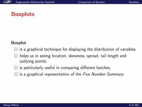
City Country Pop. (10000) Order StatisticsTokyo Japan 3420 x(15)
Mexico City Mexico 2280 x(14)
Seoul South Korea 2230 x(13)
New York USA 2190 x(12)
Sao Paulo Brazil 2020 x(11)
Bombay India 1985 x(10)
Delhi India 1970 x(9)
Shanghai China 1815 x(8)
Los Angeles USA 1800 x(7)
Osaka Japan 1680 x(6)
Jakarta Indonesia 1655 x(5)
Calcutta India 1565 x(4)
Cairo Egypt 1560 x(3)
Manila Philippines 1495 x(2)
Karachi Pakistan 1430 x(1)
Tabelle 1: The 15 largest world cities in 2006.
Ostap Okhrin 7 of 461
Angewandte Multivariate Statistik Comparison of Batches Boxplots
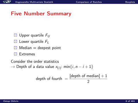
Five Number Summary
Upper quartile FU
Lower quartile FL
Median = deepest point Extremes
Consider the order statistics→ Depth of a data value x(i): mini , n − i + 1
depth of fourth =[depth of median] + 1
2
Ostap Okhrin 8 of 461
Angewandte Multivariate Statistik Comparison of Batches Boxplots
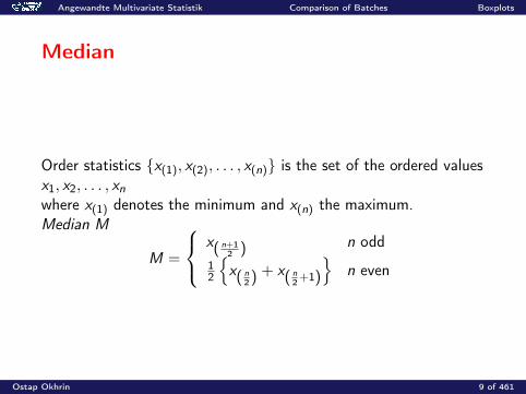
Median
Order statistics x(1), x(2), . . . , x(n) is the set of the ordered valuesx1, x2, . . . , xnwhere x(1) denotes the minimum and x(n) the maximum.Median M
M =
x( n+12 ) n odd
12
x( n
2) + x( n2+1)
n even
Ostap Okhrin 9 of 461

Angewandte Multivariate Statistik Comparison of Batches Boxplots
Construction of the Boxplot
Median: 1815 (depth of data 8)Fourths (depth = 4.5): 1610=FL, 2105=FUExtremes (depth = 1): 1430, 3420F-spread: FU − FL = dFOutside bars: FU + 1.5dF , FL − 1.5dF
1. Construct the box with borders at FU and FL
2. Draw Median as | and Mean as...
3. Draw whiskers a to data within the outside bars4. Mark outliers by • if they are outside [FL − 1.5dF ,FU + 1.5dF ]
and by ? if they lie outside [FL − 3dF ,FU + 3dF ]
Ostap Okhrin 10 of 461

1500
2000
2500
3000
World Cities
Val
ues
Boxplot
Boxplot for world cities. MVAboxcity
US JAPAN EU
1520
2530
3540
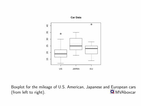
Car Data
Boxplot for the mileage of U.S. American, Japanese and European cars(from left to right). MVAboxcar
GENUINE COUNTERFEIT
138
139
140
141
142
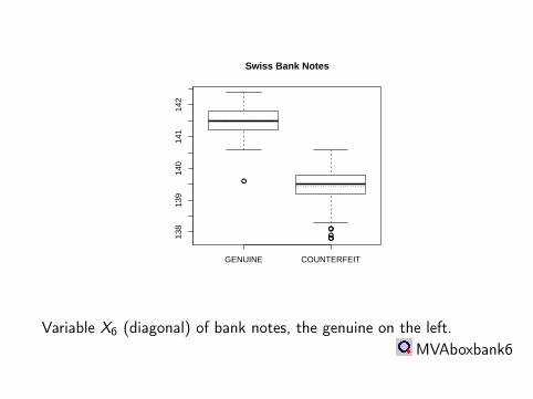
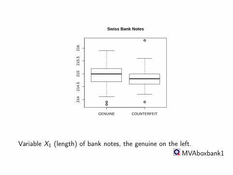
Swiss Bank Notes
Variable X6 (diagonal) of bank notes, the genuine on the left.MVAboxbank6
GENUINE COUNTERFEIT
214
214.
521
521
5.5
216
Swiss Bank Notes
Variable X1 (length) of bank notes, the genuine on the left.MVAboxbank1
Angewandte Multivariate Statistik Comparison of Batches Boxplots
Summary: Boxplots
Median and mean bars indicate the central locations. The relative location of median (and mean) in the box is a
measure of skewness. The length of the box and whiskers is a measure of spread. The length of whiskers indicate the tail length of the distribution.
Ostap Okhrin 15 of 461
Angewandte Multivariate Statistik Comparison of Batches Boxplots
Summary: Boxplots
The outliers are marked by • if they are outside[FL − 1.5dF ,FU + 1.5dF ] and by ? if they lie outside[FL − 3dF ,FU + 3dF ]
The boxplots do not indicate multi-modality or clusters. If we compare the relative size and location of the boxes, we are
comparing distributions.
Ostap Okhrin 16 of 461
Angewandte Multivariate Statistik Comparison of Batches Histograms
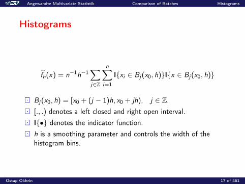
Histograms
fh(x) = n−1h−1∑j∈Z
n∑i=1
Ixi ∈ Bj(x0, h)Ix ∈ Bj(x0, h)
Bj(x0, h) = [x0 + (j − 1)h, x0 + jh), j ∈ Z. [., .) denotes a left closed and right open interval. I• denotes the indicator function. h is a smoothing parameter and controls the width of the
histogram bins.
Ostap Okhrin 17 of 461
Swiss Bank Notes
h = 0.1
Dia
gona
l
138 139 140 141
04
8
Swiss Bank Notes
h = 0.3
Dia
gona
l
138 139 140 141
010
2030
Swiss Bank Notes
h = 0.2
Dia
gona
l
138 139 140 141
05
15
Swiss Bank Notes
h = 0.4D
iago
nal
138 139 140 141
020
40
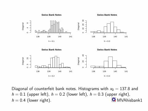
Diagonal of counterfeit bank notes. Histograms with x0 = 137.8 andh = 0.1 (upper left), h = 0.2 (lower left), h = 0.3 (upper right),h = 0.4 (lower right). MVAhisbank1
Swiss Bank Notes
x_0 = 137.65
Dia
gona
l
138 139 140 141
020
40
Swiss Bank Notes
x_0 = 137.85
Dia
gona
l
138 139 140 141
020
40
Swiss Bank Notes
x_0 = 137.75
Dia
gona
l
138 139 140 141
020
40
Swiss Bank Notes
x_0 = 137.95D
iago
nal
138 139 140 141
020
40
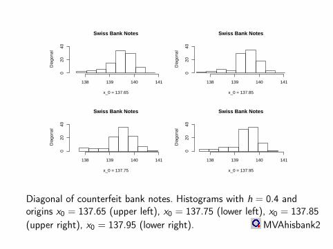
Diagonal of counterfeit bank notes. Histograms with h = 0.4 andorigins x0 = 137.65 (upper left), x0 = 137.75 (lower left), x0 = 137.85(upper right), x0 = 137.95 (lower right). MVAhisbank2

Angewandte Multivariate Statistik Comparison of Batches Histograms
Summary: Histograms
Modes of the density are detected with a histogram. Modes correspond to strong peaks in the histogram. Histograms with the same h need not be identical. They also
depend on the origin x0 of the grid. The influence of the origin x0 is drastic. Changing x0 creates
different looking histograms.
Ostap Okhrin 20 of 461
Angewandte Multivariate Statistik Comparison of Batches Histograms
Summary: Histograms
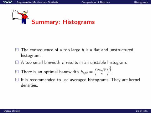
The consequence of a too large h is a flat and unstructuredhistogram.
A too small binwidth h results in an unstable histogram.
There is an optimal bandwidth hopt =(
24√π
n
) 13 .
It is recommended to use averaged histograms. They are kerneldensities.
Ostap Okhrin 21 of 461

Angewandte Multivariate Statistik Comparison of Batches Kernel densities
Kernel densities
Histogram (at the center of a bin) can be written as
fh(x) = n−1(2h)−1n∑
i=1
I(|x − xi | ≤ h)
Define K (u) = I (|u| ≤ 1/2)
fh(x) = n−1h−1n∑
i=1
K
(x − xi
h
)K is the kernel.
Ostap Okhrin 22 of 461

Angewandte Multivariate Statistik Comparison of Batches Kernel densities
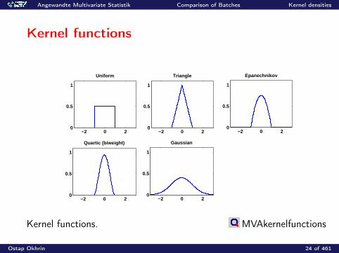
Kernel functions
K (•) Kernel
K (u) = 12 I(|u| ≤ 1) Uniform
K (u) = (1− |u|)I(|u| ≤ 1) TriangleK (u) = 3
4(1− u2)I(|u| ≤ 1) EpanechnikovK (u) = 15
16(1− u2)2I(|u| ≤ 1) Quartic (Biweight)K (u) = 1√
2πexp(−u2
2 ) = ϕ(u) Gaussian
Tabelle 2: Kernel functions.
Ostap Okhrin 23 of 461
Angewandte Multivariate Statistik Comparison of Batches Kernel densities
Kernel functions
−2 0 20
0.5
1
Uniform
−2 0 20
0.5
1
Triangle
−2 0 20
0.5
1
Epanechnikov
−2 0 20
0.5
1
Quartic (biweight)
−2 0 20
0.5
1
Gaussian
Kernel functions. MVAkernelfunctions
Ostap Okhrin 24 of 461
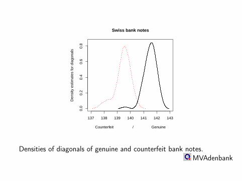
137 138 139 140 141 142 143
0.0
0.2
0.4
0.6
0.8
Swiss bank notes
Counterfeit / Genuine
Den
sity
est
imat
es fo
r di
agon
als
Densities of diagonals of genuine and counterfeit bank notes.MVAdenbank

Angewandte Multivariate Statistik Comparison of Batches Kernel densities
Choice of the bandwidth h
Silverman’s rule of thumbGaussian kernel
K (u) =1√2π
exp(−u2
2)
hG = 1.06σn−15
Quartic kernel
K (u) =1516
(1− u2)2I(|u| ≤ 1)
hQ = 2.62hG
Sample standard deviation: σ =
√n−1
n∑i=1
(xi − x)2
Ostap Okhrin 26 of 461
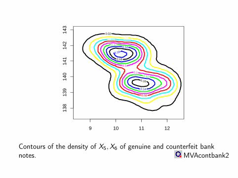
0.02 0.04 0.06
0.08
0.1
0.1
0.12
0.12
0.14
0.14
0.16
0.16
0.18
9 10 11 12
138
139
140
141
142
143
Contours of the density of X5,X6 of genuine and counterfeit banknotes. MVAcontbank2
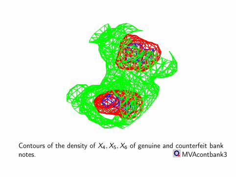
Contours of the density of X4,X5,X6 of genuine and counterfeit banknotes. MVAcontbank3

Angewandte Multivariate Statistik Comparison of Batches Kernel densities
Summary: Kernel densities
Kernel densities estimate distribution densities by the kernelmethod.
The bandwidth h determines the degree of smoothness of theestimate f .
Kernel densities are smooth functions and they can graphicallyrepresent distributions (up to 3 dimensions).
Ostap Okhrin 29 of 461

Angewandte Multivariate Statistik Comparison of Batches Kernel densities
Summary: Kernel densities
A simple (but not necessarily correct) way to find a goodbandwidth is to compute the rule of thumb bandwidthhG = 1.06σn−1/5. This bandwidth is to be used only incombination with a Gaussian kernel ϕ.
Kernel density estimates are a good descriptive tool for seeingmodes, location, skewness, tails, asymmetry, etc.
Ostap Okhrin 30 of 461
Angewandte Multivariate Statistik Comparison of Batches Scatterplots
Scatterplots
Scatterplots - bivariate or trivariate plots of variables against eachother
Rotation of data Separation lines Draftman’s plot Brushing Parallel coordinate plots
Ostap Okhrin 31 of 461
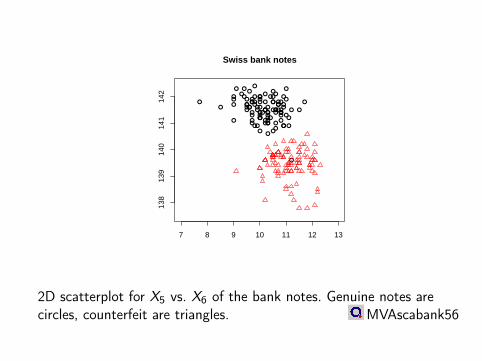
7 8 9 10 11 12 13
138
139
140
141
142
Swiss bank notes
2D scatterplot for X5 vs. X6 of the bank notes. Genuine notes arecircles, counterfeit are triangles. MVAscabank56
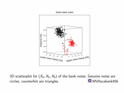
Swiss bank notes
8 10 11 13 14 8 9 10 11 12
139
140
140
141
142
Lower inner frame (X4) Upper inner frame (X5)
Dia
gona
l (X
6)
3D scatterplot for (X4,X5,X6) of the bank notes. Genuine notes arecircles, counterfeit are triangles. MVAscabank456
3
X
Y
128.5 129.0 129.5 130.0 130.5 131.0 131.5
78
910
1112
13
X
Y
128.5 129.0 129.5 130.0 130.5 131.0 131.5
78
910
1112
13
X
Y
128.5 129.0 129.5 130.0 130.5 131.0 131.5
137
138
139
140
141
142
143
7 8 9 10 11 12
129.
012
9.5
130.
013
0.5
131.
0
X
Y
4
X
Y
7 8 9 10 11 12 13
78
910
1112
13
X
Y
7 8 9 10 11 12 13
137
138
139
140
141
142
143
8 9 10 11 12
129.
012
9.5
130.
013
0.5
131.
0
X
Y
8 9 10 11 12
78
910
1112
X
Y
5
X
Y
7 8 9 10 11 12 13
137
138
139
140
141
142
143
138 139 140 141 142
129.
012
9.5
130.
013
0.5
131.
0
X
Y
138 139 140 141 142
78
910
1112
X
Y
138 139 140 141 142
89
1011
12
X
Y
6
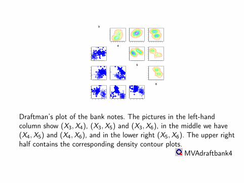
Draftman’s plot of the bank notes. The pictures in the left-handcolumn show (X3,X4), (X3,X5) and (X3,X6), in the middle we have(X4,X5) and (X4,X6), and in the lower right (X5,X6). The upper righthalf contains the corresponding density contour plots.
MVAdraftbank4

Angewandte Multivariate Statistik Comparison of Batches Scatterplots
Summary: Scatterplots
Scatterplots in two and three dimensions help us in seeingseparated points, clouds or sub-clusters.
They help us in judging positive or negative dependence. Draftman scatterplot matrices are useful for detecting structures
conditioned on values of certain other variables. As the brush of a scatterplot matrix is moving in the point cloud
we can study conditional dependence.
Ostap Okhrin 35 of 461
Angewandte Multivariate Statistik Comparison of Batches Chernoff-Flury faces
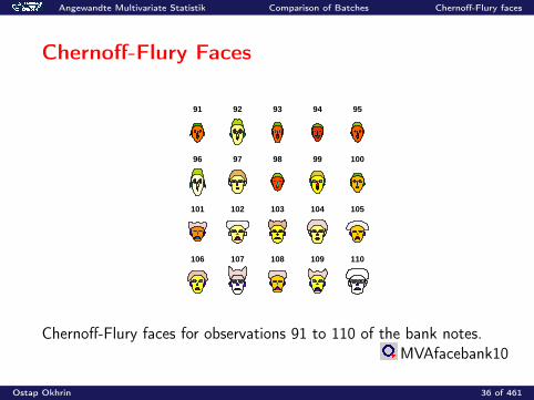
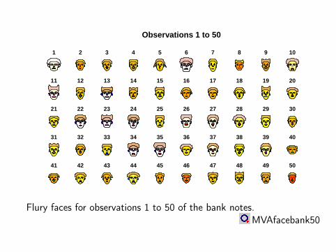
Chernoff-Flury Faces
Index
91
Index
92
Index
93
Index
94
Index
95
Index
96
Index
97
Index
98
Index
99
Index
100
Index
101
Index
102
Index
103
Index
104
Index
105
Index
106
Index
107
Index
108
Index
109
Index
110
Chernoff-Flury faces for observations 91 to 110 of the bank notes.MVAfacebank10
Ostap Okhrin 36 of 461

Angewandte Multivariate Statistik Comparison of Batches Chernoff-Flury faces
Six variables - face elements
X1 = 1, 19 (eye sizes)X2 = 2, 20 (pupil sizes)X3 = 4, 22 (eye slants)X4 = 11, 29 (upper hair lines)X5 = 12, 30 (lower hair lines)X6 = 13, 14, 31, 32 (face lines and darkness of hair)
Ostap Okhrin 37 of 461
Index
1
Index
2
Index
3
Index
4
Index
5
Index
6
Index
7
Index
8
Index
9
Index
10
Index
11
Index
12
Index
13
Index
14
Index
15
Index
16
Index
17
Index
18
Index
19
Index
20
Index
21
Index
22
Index
23
Index
24
Index
25
Index
26
Index
27
Index
28
Index
29
Index
30
Index
31
Index
32
Index
33
Index
34
Index
35
Index
36
Index
37
Index
38
Index
39
Index
40
Index
41
Index
42
Index
43
Index
44
Index
45
Index
46
Index
47
Index
48
Index
49
Index
50
Observations 1 to 50
Flury faces for observations 1 to 50 of the bank notes.MVAfacebank50
Index
51
Index
52
Index
53
Index
54
Index
55
Index
56
Index
57
Index
58
Index
59
Index
60
Index
61
Index
62
Index
63
Index
64
Index
65
Index
66
Index
67
Index
68
Index
69
Index
70
Index
71
Index
72
Index
73
Index
74
Index
75
Index
76
Index
77
Index
78
Index
79
Index
80
Index
81
Index
82
Index
83
Index
84
Index
85
Index
86
Index
87
Index
88
Index
89
Index
90
Index
91
Index
92
Index
93
Index
94
Index
95
Index
96
Index
97
Index
98
Index
99
Index
100
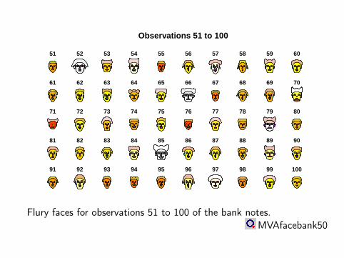
Observations 51 to 100
Flury faces for observations 51 to 100 of the bank notes.MVAfacebank50
Index
101
Index
102
Index
103
Index
104
Index
105
Index
106
Index
107
Index
108
Index
109
Index
110
Index
111
Index
112
Index
113
Index
114
Index
115
Index
116
Index
117
Index
118
Index
119
Index
120
Index
121
Index
122
Index
123
Index
124
Index
125
Index
126
Index
127
Index
128
Index
129
Index
130
Index
131
Index
132
Index
133
Index
134
Index
135
Index
136
Index
137
Index
138
Index
139
Index
140
Index
141
Index
142
Index
143
Index
144
Index
145
Index
146
Index
147
Index
148
Index
149
Index
150
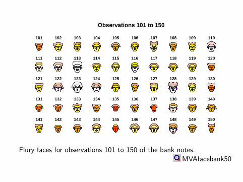
Observations 101 to 150
Flury faces for observations 101 to 150 of the bank notes.MVAfacebank50
Index
151
Index
152
Index
153
Index
154
Index
155
Index
156
Index
157
Index
158
Index
159
Index
160
Index
161
Index
162
Index
163
Index
164
Index
165
Index
166
Index
167
Index
168
Index
169
Index
170
Index
171
Index
172
Index
173
Index
174
Index
175
Index
176
Index
177
Index
178
Index
179
Index
180
Index
181
Index
182
Index
183
Index
184
Index
185
Index
186
Index
187
Index
188
Index
189
Index
190
Index
191
Index
192
Index
193
Index
194
Index
195
Index
196
Index
197
Index
198
Index
199
Index
200
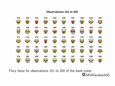
Observations 151 to 200
Flury faces for observations 151 to 200 of the bank notes.MVAfacebank50

Angewandte Multivariate Statistik Comparison of Batches Chernoff-Flury faces
Summary: Faces
Faces can be used to detect subgroups in multivariate data. Subgroups are characterized by similar looking faces. Outliers are identified by extreme faces (e.g. dark hair, smile or
happy face). If one element of X is unusual, the corresponding face element
changes significantly in shape.
Ostap Okhrin 42 of 461
Angewandte Multivariate Statistik Comparison of Batches Andrews’ Curves
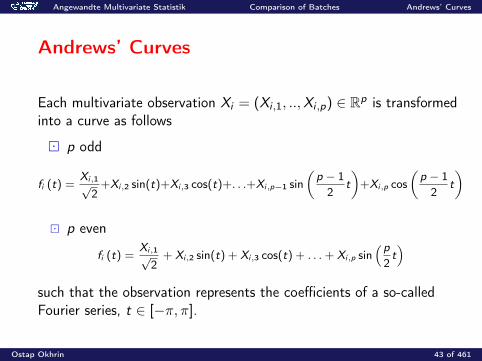
Andrews’ Curves
Each multivariate observation Xi = (Xi ,1, ..,Xi ,p) ∈ Rp is transformedinto a curve as follows
p odd
fi (t) =Xi,1√
2+Xi,2 sin(t)+Xi,3 cos(t)+. . .+Xi,p−1 sin
(p − 1
2t
)+Xi,p cos
(p − 1
2t
)
p even
fi (t) =Xi,1√
2+ Xi,2 sin(t) + Xi,3 cos(t) + . . .+ Xi,p sin
(p2t)
such that the observation represents the coefficients of a so-calledFourier series, t ∈ [−π, π].
Ostap Okhrin 43 of 461
Angewandte Multivariate Statistik Comparison of Batches Andrews’ Curves
Andrews’ Curves
Subgroups are characterized by similar curves. Outliers are characterized by single curves. Order plays an important role in the interpretation.
Ostap Okhrin 44 of 461

Angewandte Multivariate Statistik Comparison of Batches Andrews’ Curves
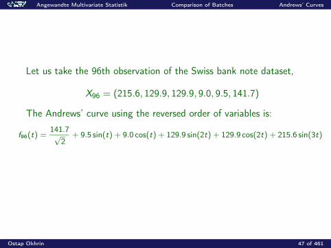
Let us take the 96th observation of the Swiss bank note dataset,
X96 = (215.6, 129.9, 129.9, 9.0, 9.5, 141.7)
The Andrews’ curve is:
f96(t) =215.6√
2+ 129.9 sin(t) + 129.9 cos(t) + 9.0 sin(2t) + 9.5 cos(2t) + 141.7 sin(3t)
Ostap Okhrin 45 of 461
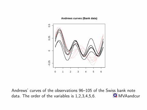
Andrews curves (Bank data)
−0.
250
0.25
0.5
0 1 2 3 4 5 6
Andrews’ curves of the observations 96–105 of the Swiss bank notedata. The order of the variables is 1,2,3,4,5,6. MVAandcur
Angewandte Multivariate Statistik Comparison of Batches Andrews’ Curves
Let us take the 96th observation of the Swiss bank note dataset,
X96 = (215.6, 129.9, 129.9, 9.0, 9.5, 141.7)
The Andrews’ curve using the reversed order of variables is:
f96(t) =141.7√
2+ 9.5 sin(t) + 9.0 cos(t) + 129.9 sin(2t) + 129.9 cos(2t) + 215.6 sin(3t)
Ostap Okhrin 47 of 461
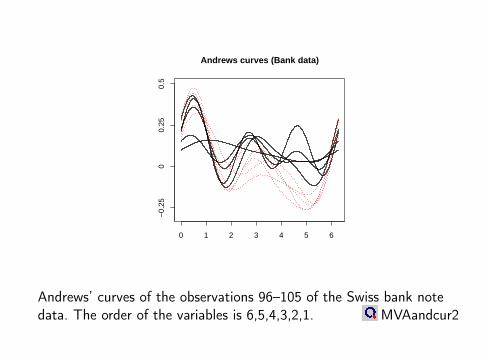
Andrews curves (Bank data)
−0.
250
0.25
0.5
0 1 2 3 4 5 6
Andrews’ curves of the observations 96–105 of the Swiss bank notedata. The order of the variables is 6,5,4,3,2,1. MVAandcur2
Angewandte Multivariate Statistik Comparison of Batches Andrews’ Curves
Summary: Andrews’ Curves
Outliers appear as single Andrew’s curves, which looks differentfrom the rest.
A subgroup is characterized by a set of similar curves. The order of the variables plays an important role for
interpretation. The order of variables may be optimized by Principal Component
Analysis. For more than 20 observations we obtain a bad ”signal-to-ink-
ratio”, which means we cannot see the structure of so manycurves obtained.
Ostap Okhrin 49 of 461

Angewandte Multivariate Statistik Comparison of Batches Parallel coordinate plots
Parallel Coordinate Plots
Parallel Coordinate Plots Are not based on an orthogonal coordinate system Allow to see more than four dimensions
IdeaInstead of plotting observations in an orthogonal coordinate systemone draws their coordinates in a system of parallel axes. This way ofrepresentation is however sensitive to the order of the variables.
Ostap Okhrin 50 of 461
Parallel coordinates plot (Bank data)
V1 V2 V3 V4 V5 V6
00.
20.
40.
60.
81
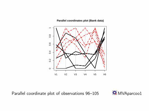
Parallel coordinate plot of observations 96–105 MVAparcoo1
Parallel coordinates plot (Bank data)
V1 V2 V3 V4 V5 V6
00.
20.
40.
60.
81
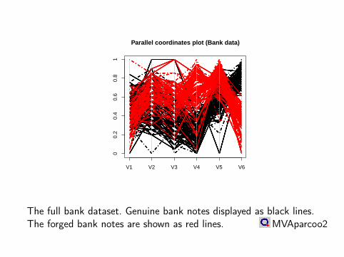
The full bank dataset. Genuine bank notes displayed as black lines.The forged bank notes are shown as red lines. MVAparcoo2

Angewandte Multivariate Statistik Comparison of Batches Parallel coordinate plots
Summary: Parallel coordinate plots
Parallel coordinate plots overcome the visualisation problem ofthe Cartesian coordinate system for dimensions greater than 4.
Outliers are seen as outlying polygon curves. The order of variables is still important for detection of subgroups. Subgroups may be screened by selective coloring in an interactive
manner.
Ostap Okhrin 53 of 461

Angewandte Multivariate Statistik A Short Excursion into Matrix Algebra Elementary Operations
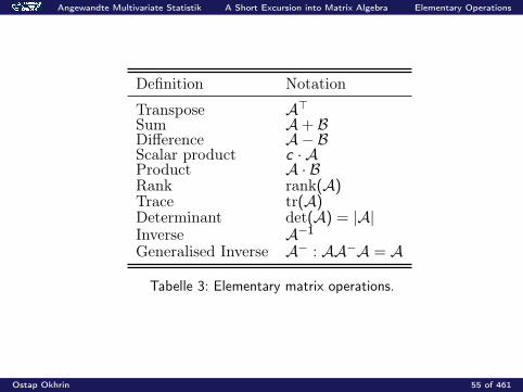
A Short Excursion into Matrix Algebra
A(n×p) =
a11 · · · a1p...
. . ....
an1 · · · anp
Ostap Okhrin 54 of 461
Angewandte Multivariate Statistik A Short Excursion into Matrix Algebra Elementary Operations
Definition Notation
Transpose A>Sum A+ BDifference A− BScalar product c · AProduct A · BRank rank(A)Trace tr(A)Determinant det(A) = |A|Inverse A−1
Generalised Inverse A− : AA−A = A
Tabelle 3: Elementary matrix operations.
Ostap Okhrin 55 of 461

Angewandte Multivariate Statistik A Short Excursion into Matrix Algebra Elementary Operations
Name Definition Notation Example
scalar p = n = 1 a 3
column vector p = 1 a
(13
)row vector n = 1 a>
(1 3
)vector of ones (1, . . . , 1︸ ︷︷ ︸
n
)> 1n
(11
)vector of zeros (0, . . . , 0︸ ︷︷ ︸
n
)> 0n
(00
)square matrix n = p A(p × p)
(2 00 2
)Tabelle 4: Special matrices and vectors.
Ostap Okhrin 56 of 461
Angewandte Multivariate Statistik A Short Excursion into Matrix Algebra Elementary Operations
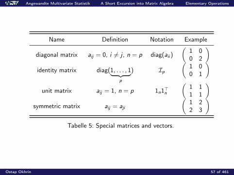
Name Definition Notation Example
diagonal matrix aij = 0, i 6= j , n = p diag(aii )
(1 00 2
)identity matrix diag(1, . . . , 1︸ ︷︷ ︸
p
) Ip(
1 00 1
)unit matrix aij = 1, n = p 1n1>n
(1 11 1
)symmetric matrix aij = aji
(1 22 3
)Tabelle 5: Special matrices and vectors.
Ostap Okhrin 57 of 461
Angewandte Multivariate Statistik A Short Excursion into Matrix Algebra Elementary Operations
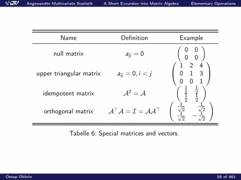
Name Definition Example
null matrix aij = 0(
0 00 0
)upper triangular matrix aij = 0, i < j
1 2 40 1 30 0 1
idempotent matrix A2 = A
( 12
12
12
12
)orthogonal matrix A>A = I = AA>
(1√2
1√2
1√2− 1√
2
)
Tabelle 6: Special matrices and vectors.
Ostap Okhrin 58 of 461
Angewandte Multivariate Statistik A Short Excursion into Matrix Algebra Elementary Operations
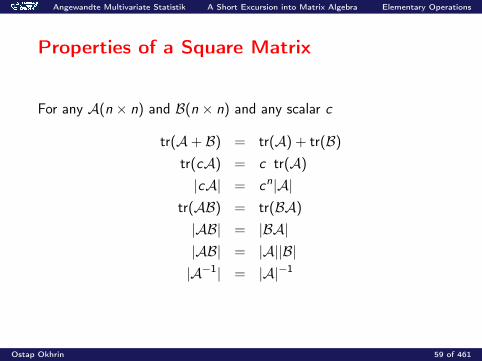
Properties of a Square Matrix
For any A(n × n) and B(n × n) and any scalar c
tr(A+ B) = tr(A) + tr(B)
tr(cA) = c tr(A)
|cA| = cn|A|tr(AB) = tr(BA)
|AB| = |BA||AB| = |A||B||A−1| = |A|−1
Ostap Okhrin 59 of 461
Angewandte Multivariate Statistik A Short Excursion into Matrix Algebra Elementary Operations
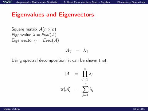
Eigenvalues and Eigenvectors
Square matrix A(n × n)Eigenvalue λ = Eval(A)Eigenvector γ = Evec(A)
Aγ = λγ
Using spectral decomposition, it can be shown that:
|A| =n∏
j=1
λj
tr(A) =n∑
j=1
λj
Ostap Okhrin 60 of 461

Angewandte Multivariate Statistik A Short Excursion into Matrix Algebra Elementary Operations
Summary: Matrix Algebra
The determinant |A| is a product of the eigenvalues of A. The inverse of a matrix A exists if |A| 6= 0. The trace tr(A) is the sum of the eigenvalues of A. The sum of the traces of two matrices equals the trace of the
sum of the two matrices. The trace tr(AB) equals tr(BA). The rank(A) is the maximum number of linearly independent
rows (columns) of A .
Ostap Okhrin 61 of 461
Angewandte Multivariate Statistik A Short Excursion into Matrix Algebra Spectral Decomposition
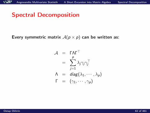
Spectral Decomposition
Every symmetric matrix A(p × p) can be written as:
A = ΓΛΓ>
=
p∑j=1
λjγjγ>j
Λ = diag(λ1, · · · , λp)
Γ = (γ1, · · · , γp)
Ostap Okhrin 62 of 461
Angewandte Multivariate Statistik A Short Excursion into Matrix Algebra Spectral Decomposition
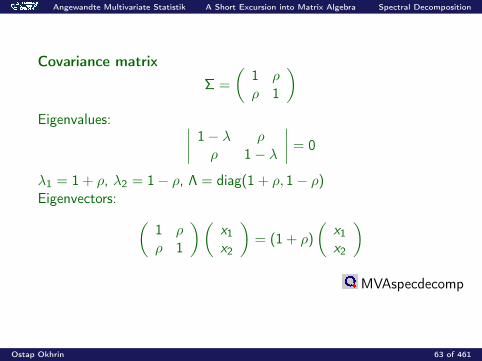
Covariance matrix
Σ =
(1 ρρ 1
)Eigenvalues: ∣∣∣∣ 1− λ ρ
ρ 1− λ
∣∣∣∣ = 0
λ1 = 1 + ρ, λ2 = 1− ρ, Λ = diag(1 + ρ, 1− ρ)Eigenvectors: (
1 ρρ 1
)(x1x2
)= (1 + ρ)
(x1x2
)MVAspecdecomp
Ostap Okhrin 63 of 461
Angewandte Multivariate Statistik A Short Excursion into Matrix Algebra Spectral Decomposition
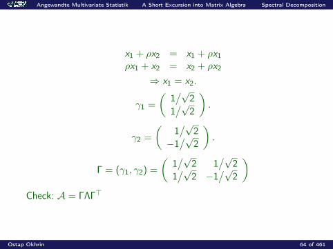
x1 + ρx2 = x1 + ρx1ρx1 + x2 = x2 + ρx2
⇒ x1 = x2.
γ1 =
(1/√
21/√
2
).
γ2 =
(1/√
2−1/√
2
).
Γ = (γ1, γ2) =
(1/√
2 1/√
21/√
2 −1/√
2
)Check: A = ΓΛΓ>
Ostap Okhrin 64 of 461
Angewandte Multivariate Statistik A Short Excursion into Matrix Algebra Spectral Decomposition
Eigenvectors
The direction of the first eigenvector is the main direction of the pointcloud. The second eigenvector is orthogonal to the first one.
This eigenvector direction is in general different from the LSregression shape line.
Ostap Okhrin 65 of 461
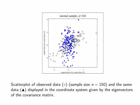
normal sample, n=150
-2 0 2
original data (x1), rotated data (x1)
-20
24
orig
inal
dat
a (y
2), r
otat
ed d
ata
(y2)
Scatterplot of observed data () (sample size n = 150) and the samedata (N) displayed in the coordinate system given by the eigenvectorsof the covariance matrix.
Angewandte Multivariate Statistik A Short Excursion into Matrix Algebra Spectral Decomposition
Singular Value Decomposition (SVD)
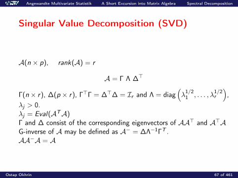
A(n × p), rank(A) = r
A = Γ Λ ∆>
Γ(n× r), ∆(p × r), Γ>Γ = ∆>∆ = Ir and Λ = diag(λ
1/21 , . . . , λ
1/2r
),
λj > 0.λj = Eval(ATA)Γ and ∆ consist of the corresponding eigenvectors of AA> and A>AG-inverse of A may be defined as A− = ∆Λ−1ΓT .AA−A = A
Ostap Okhrin 67 of 461
Angewandte Multivariate Statistik A Short Excursion into Matrix Algebra Spectral Decomposition
Summary: Spectral Decomposition
The spectral (Jordan) decomposition gives a representation of asymmetric matrix in terms of eigenvalues and eigenvectors.
The eigenvectors belonging to the largest eigenvalues point intothe "main directionöf the data.
The Jordan decomposition allows to easily compute the power ofa matrix A: Aα = ΓΛαΓ>.
A−1 = ΓΛ−1Γ>, A1/2 = ΓΛ1/2Γ>.
Ostap Okhrin 68 of 461
Angewandte Multivariate Statistik A Short Excursion into Matrix Algebra Spectral Decomposition
Summary: Spectral Decomposition
The singular value decomposition (SVD) is a generalization of theJordan decomposition to non-quadratic matrices.
The direction of the first eigenvector of the covariance matrix of atwo-dimensional point cloud is different from the least squaresregression line.
Ostap Okhrin 69 of 461
Angewandte Multivariate Statistik A Short Excursion into Matrix Algebra Quadratic Forms
Quadratic Forms
A(p × p) symmetric matrix can be written as
Q(x) = x>Ax =
p∑i=1
p∑j=1
aijxixj
Definiteness
Q(x) > 0 for all x 6= 0 positive definite (pd),Q(x) ≥ 0 for all x 6= 0 positive semidefinite (psd).
A is pd (psd) iff Q(x) = x>Ax is pd (psd).
Ostap Okhrin 70 of 461

Angewandte Multivariate Statistik A Short Excursion into Matrix Algebra Quadratic Forms
Example:Q(x) = x>Ax = x2
1 + x22 , A =
(10
01
)Eigenvalues: λ1 = λ2 = 1 positive definiteQ(x) = (x1 − x2)2, A =
(1−1−1
1
)Eigenvalues λ1 = 2, λ2 = 0 positive semidefiniteQ(x) = x2
1 − x22
Eigenvalues λ1 = 1, λ2 = −1 indefinite.
Ostap Okhrin 71 of 461
Angewandte Multivariate Statistik A Short Excursion into Matrix Algebra Quadratic Forms
TheoremIf A is symmetric and Q(x) = x>Ax is the corresponding quadraticform, then there exists a transformation x 7→ Γ>x = y such that
x> A x =
p∑i=1
λiy2i ,
where λi are the eigenvalues of A.Lemma
A > 0 ⇔ λi > 0,A ≥ 0 ⇔ λi ≥ 0, i = 1, . . . , p.
Ostap Okhrin 72 of 461

Angewandte Multivariate Statistik A Short Excursion into Matrix Algebra Quadratic Forms
Theorem (Theorem 2.5)If A and B are symmetric and B > 0, then the maximum of x>Ax
x>Bx isgiven by the largest eigenvalue of B−1A. More generally,
maxx
x>Axx>Bx
= λ1 ≥ λ2 ≥ · · · ≥ λp = minx
x>Axx>Bx
,
where λ1, . . . , λp denote the eigenvalues of B−1A. The vector whichmaximises (minimises) x>Ax
x>Bx is the eigenvector of B−1A whichcorresponds to the largest (smallest) eigenvalue of B−1A. Ifx>Bx = 1, we get
maxx
x>Ax = λ1 ≥ λ2 ≥ · · · ≥ λp = minx
x>Ax
Ostap Okhrin 73 of 461

Angewandte Multivariate Statistik A Short Excursion into Matrix Algebra Quadratic Forms
Summary: Quadratic forms
A quadratic form can be described by a symmetric quadraticmatrix A.
Quadratic forms can always be diagonalized. Positive definiteness of a quadratic form is equivalent to
positiveness of the eigenvalues of the matrix A. The maximum and minimum of a quadratic form under
constraints can be expressed in terms of eigenvalues.
Ostap Okhrin 74 of 461
Angewandte Multivariate Statistik A Short Excursion into Matrix Algebra Derivatives
Derivatives
f : Rp → R, (p × 1) vector x :
∂f (x)
∂xcolumn vector of partial derivatives
∂f (x)
∂xj
, j = 1, . . . , p
∂f (x)
∂x>row vector of the same derivatives
∂f (x)
∂xis called the gradient of f .
Ostap Okhrin 75 of 461
Angewandte Multivariate Statistik A Short Excursion into Matrix Algebra Derivatives
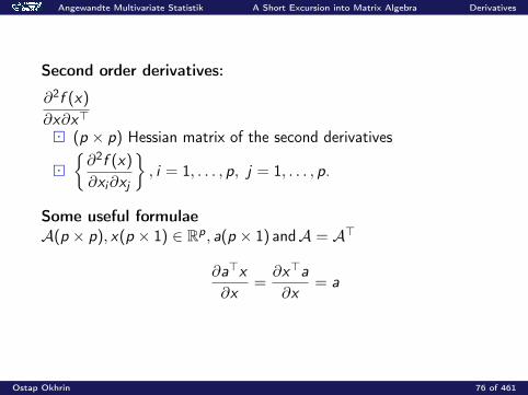
Second order derivatives:
∂2f (x)
∂x∂x>
(p × p) Hessian matrix of the second derivatives
∂2f (x)
∂xi∂xj
, i = 1, . . . , p, j = 1, . . . , p.
Some useful formulaeA(p × p), x(p × 1) ∈ Rp, a(p × 1) andA = A>
∂a>x
∂x=∂x>a
∂x= a
Ostap Okhrin 76 of 461

Angewandte Multivariate Statistik A Short Excursion into Matrix Algebra Derivatives
Example:f : Rp → R, f (x) = a>x
a = (1, 2)>, x = (x1, x2)>
∂a>x
∂x=∂(x1 + 2x2)
∂x= (1, 2)> = a
Ostap Okhrin 77 of 461

Angewandte Multivariate Statistik A Short Excursion into Matrix Algebra Derivatives
Derivatives of the quadratic form
∂x>Ax∂x
= 2Ax
∂2x>Ax∂x∂x>
= 2A
Ostap Okhrin 78 of 461
Angewandte Multivariate Statistik A Short Excursion into Matrix Algebra Derivatives
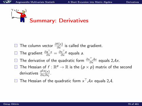
Summary: Derivatives
The column vector ∂f (x)∂x is called the gradient.
The gradient ∂a>x∂x = ∂x>a
∂x equals a.
The derivative of the quadratic form ∂x>Ax∂x equals 2Ax .
The Hessian of f : Rp → R is the (p × p) matrix of the secondderivatives ∂2f (x)
∂xi∂xj.
The Hessian of the quadratic form x>Ax equals 2A.
Ostap Okhrin 79 of 461

Angewandte Multivariate Statistik A Short Excursion into Matrix Algebra Partitioned Matrices
Partitioned Matrices
A(n × p),B(n × p), A =
(A11 A12A21 A22
)Aij(ni × pj), n1 + n2 = n and p1 + p2 = p
A+ B =
(A11 + B11 A12 + B12A21 + B21 A22 + B22
)B> =
(B>11 B>21B>12 B>22
)AB> =
(A11B>11 +A12B>12 A11B>21 +A12B>22A21B>11 +A22B>12 A21B>21 +A22B>22
)
Ostap Okhrin 80 of 461
Angewandte Multivariate Statistik A Short Excursion into Matrix Algebra Partitioned Matrices
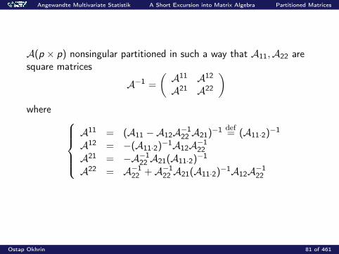
A(p × p) nonsingular partitioned in such a way that A11,A22 aresquare matrices
A−1 =
(A11 A12
A21 A22
)where
A11 = (A11 −A12A−122 A21)−1 def
= (A11·2)−1
A12 = −(A11·2)−1A12A−122
A21 = −A−122 A21(A11·2)−1
A22 = A−122 +A−1
22 A21(A11·2)−1A12A−122
Ostap Okhrin 81 of 461
Angewandte Multivariate Statistik A Short Excursion into Matrix Algebra Partitioned Matrices
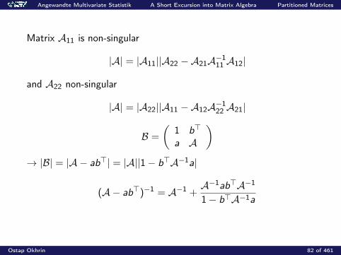
Matrix A11 is non-singular
|A| = |A11||A22 −A21A−111 A12|
and A22 non-singular
|A| = |A22||A11 −A12A−122 A21|
B =
(1 b>
a A
)→ |B| = |A − ab>| = |A||1− b>A−1a|
(A− ab>)−1 = A−1 +A−1ab>A−1
1− b>A−1a
Ostap Okhrin 82 of 461
Angewandte Multivariate Statistik A Short Excursion into Matrix Algebra Partitioned Matrices
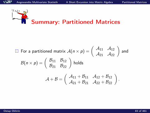
Summary: Partitioned Matrices
For a partitioned matrix A(n × p) =
(A11 A12A21 A22
)and
B(n × p) =
(B11 B12B21 B22
)holds
A+ B =
(A11 + B11 A12 + B12A21 + B21 A22 + B22
).
Ostap Okhrin 83 of 461

Angewandte Multivariate Statistik A Short Excursion into Matrix Algebra Partitioned Matrices
Summary: Partitioned Matrices
The product AB> equals(A11B>11 +A12B>12 A11B>21 +A12B>22A21B>11 +A22B>12 A21B>21 +A22B>22
).
Ostap Okhrin 84 of 461
Angewandte Multivariate Statistik A Short Excursion into Matrix Algebra Partitioned Matrices
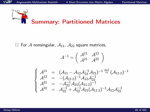
Summary: Partitioned Matrices
For A nonsingular, A11, A22 square matrices,
A−1 =
(A11 A12
A21 A22
)A11 = (A11 −A12A−1
22 A21)−1 def= (A11·2)−1
A12 = −(A11·2)−1A12A−122
A21 = −A−122 A21(A11·2)−1
A22 = A−122 +A−1
22 A21(A11·2)−1A12A−122
Ostap Okhrin 85 of 461

Angewandte Multivariate Statistik A Short Excursion into Matrix Algebra Partitioned Matrices
Summary: Partitioned Matrices
For B =
(1 b>
a A
)and for non-singular A we have
|B| = |A − ab>| = |A||1− b>A−1a|. (A− ab>)−1 = A−1 + A−1ab>A−1
1−b>A−1a
Ostap Okhrin 86 of 461
Angewandte Multivariate Statistik A Short Excursion into Matrix Algebra Geometrical Aspects
Geometrical Aspects
Distance function d : R2p → R+
d2(x , y) = (x − y)>A(x − y), A > 0
A = Ip, Euclidean distance
Ed = x ∈ Rp | (x − x0)>(x − x0) = d2
Example: x ∈ R2, x0 = 0, x21 + x2
2 = 1Norm of a vector w.r.t metric Ip
‖x‖Ip = d(0, x) =√x>x
Ostap Okhrin 87 of 461
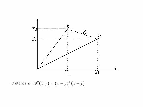
Distance d . d2(x , y) = (x − y)>(x − y)
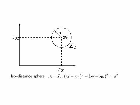
Iso–distance sphere. A = I2, (x1 − x01)2 + (x2 − x02)2 = d2
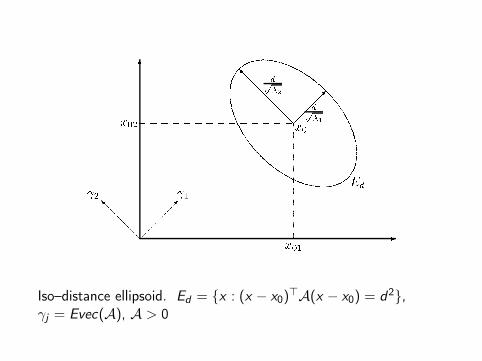
Iso–distance ellipsoid. Ed = x : (x − x0)>A(x − x0) = d2,γj = Evec(A), A > 0

Angewandte Multivariate Statistik A Short Excursion into Matrix Algebra Geometrical Aspects
Angle between Vectors
Scalar product
< x , y > = x>y
< x , y >A = x>Ay
Norm of a vector
‖x‖Ip = d(0, x) =√x>x
‖x‖A =√x>Ax
Unit vectorsx : ‖x‖ = 1
Ostap Okhrin 91 of 461

Angewandte Multivariate Statistik A Short Excursion into Matrix Algebra Geometrical Aspects
Angle between Two Vectors
Angle of vectors x and y can be calculated as
cos θ =x>y
‖x‖ ‖y‖
Example: Angle = CorrelationObservations xini=1, yini=1x = y = 0
rXY =
∑xiyi√∑x2i
∑y2i
= cos θ
Correlation corresponds to the angle between x , y ∈ Rn.
Ostap Okhrin 92 of 461
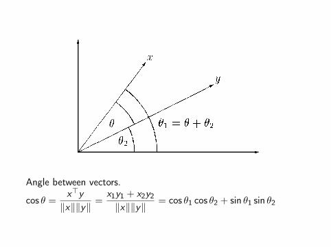
Angle between vectors.
cos θ =x>y
‖x‖‖y‖=
x1y1 + x2y2
‖x‖‖y‖= cos θ1 cos θ2 + sin θ1 sin θ2

Angewandte Multivariate Statistik A Short Excursion into Matrix Algebra Geometrical Aspects
Column space
X (n × p) data matrix
C (X ) = x ∈ Rn | ∃a ∈ Rp so that X a = x
Projection matrixP(n × n), P = P> = P2 (P is idempotent)let b ∈ Rn, a = Pb is the projection of b on C (P)
Ostap Okhrin 94 of 461

Angewandte Multivariate Statistik A Short Excursion into Matrix Algebra Geometrical Aspects
Projection on C (X )
X (n × p), P = X (X>X )−1X>
PX = X , P is a projector, PP = P.
Q = In − P,Q2 = Q
px =y>x
‖y‖2y
PX = XQX = 0
Ostap Okhrin 95 of 461
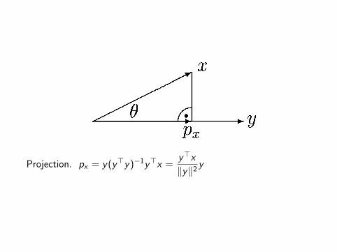
Projection. px = y(y>y)−1y>x =y>x
‖y‖2y

Angewandte Multivariate Statistik A Short Excursion into Matrix Algebra Geometrical Aspects
Summary: Geometrical aspects
A distance between two p-dimensional points x , y is a quadraticform (x − y)>A(x − y) in the vectors of differences (x − y). Adistance defines the norm of a vector.
Iso-distance curves of a point x0 are all those points which havethe same distance from x0. Iso-distance curves are ellipsoidswhose principal axes are determined by the direction of theeigenvectors. The half-length of principal axes is proportional tothe inverse of the roots of the eigenvalues of A.
Ostap Okhrin 97 of 461
Angewandte Multivariate Statistik A Short Excursion into Matrix Algebra Geometrical Aspects
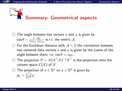
Summary: Geometrical aspects
The angle between two vectors x and y is given bycos θ = x>Ay
‖x‖A ‖y‖A w.r.t. the metric A. For the Euclidean distance with A = I the correlation between
two centered data vectors x and y is given by the cosine of theangle between them, i.e. cos θ = rXY .
The projection P = X (X>X )−1X> is the projection onto thecolumn space C (X ) of X .
The projection of x ∈ Rn on y ∈ Rn is given bypx = y>x
‖y‖2 y .
Ostap Okhrin 98 of 461
Angewandte Multivariate Statistik Moving to Higher Dimensions Covariance
Covariance
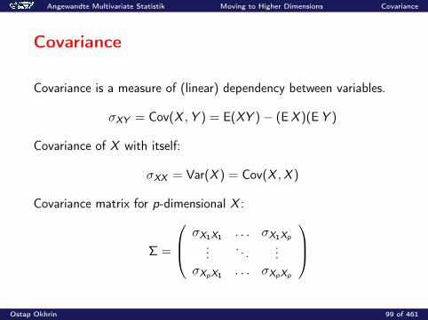
Covariance is a measure of (linear) dependency between variables.
σXY = Cov(X ,Y ) = E(XY )− (EX )(EY )
Covariance of X with itself:
σXX = Var(X ) = Cov(X ,X )
Covariance matrix for p-dimensional X :
Σ =
σX1X1 . . . σX1Xp
.... . .
...σXpX1 . . . σXpXp
Ostap Okhrin 99 of 461
Angewandte Multivariate Statistik Moving to Higher Dimensions Covariance
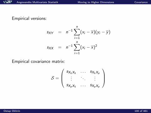
Empirical versions:
sXY = n−1n∑
i=1
(xi − x)(yi − y)
sXX = n−1n∑
i=1
(xi − x)2
Empirical covariance matrix:
S =
sX1X1 . . . sX1Xp
.... . .
...sXpX1 . . . sXpXp
Ostap Okhrin 100 of 461

Angewandte Multivariate Statistik Moving to Higher Dimensions Covariance
Example: Swiss bank data
X1 = length of the billX2 = height of the bill (left)X3 = height of the bill (right)X4 = distance of the inner frame to the lower borderX5 = distance of the inner frame to the upper borderX6 = length of the diagonal of the central picture.
Ostap Okhrin 101 of 461
Angewandte Multivariate Statistik Moving to Higher Dimensions Covariance
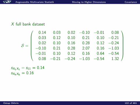
X full bank dataset
S =
0.14 0.03 0.02 −0.10 −0.01 0.080.03 0.12 0.10 0.21 0.10 −0.210.02 0.10 0.16 0.28 0.12 −0.24−0.10 0.21 0.28 2.07 0.16 −1.03−0.01 0.10 0.12 0.16 0.64 −0.540.08 −0.21 −0.24 −1.03 −0.54 1.32
sX1X1 = s11 = 0.14sX4X5 = 0.16
Ostap Okhrin 102 of 461

Angewandte Multivariate Statistik Moving to Higher Dimensions Covariance
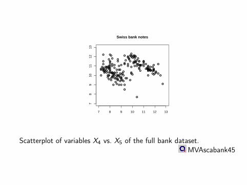
Scatterplots with point clouds that are ”upward-sloping” areshowing variables with positive covariance.
Scatterplots with ”downward-sloping” structure are showingnegative covariance.
Ostap Okhrin 103 of 461
7 8 9 10 11 12 13
78
910
1112
13
Swiss bank notes
Scatterplot of variables X4 vs. X5 of the full bank dataset.MVAscabank45

Angewandte Multivariate Statistik Moving to Higher Dimensions Covariance
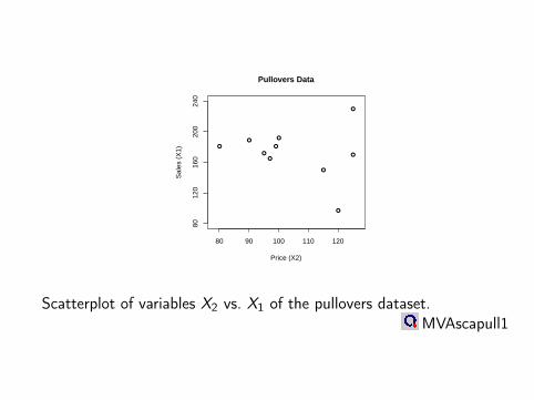
Example: “classic blue” pulloverSales of “classic blue” pullovers in 10 periods.X1 number of pullovers soldX2 price in EURX3 advertisement cost in EURX4 presence of sales assistant in hours per periodDoes price have a big influence on pullovers sold?sX1X2 = −80.02
Ostap Okhrin 105 of 461
Pullovers Data
Price (X2)
Sal
es (
X1)
8012
016
020
024
0
80 90 100 110 120
Scatterplot of variables X2 vs. X1 of the pullovers dataset.MVAscapull1
Angewandte Multivariate Statistik Moving to Higher Dimensions Covariance
Summary: Covariance
The covariance is a measure of dependence. Covariance measures only linear dependence. There are nonlinear dependencies that have zero covariance. Zero covariance does not imply independence. Independence implies zero covariance. Covariance is scale dependent.
Ostap Okhrin 107 of 461
Angewandte Multivariate Statistik Moving to Higher Dimensions Covariance
Summary: Covariance
Negative covariance corresponds to downward-slopingscatterplots.
Positive covariance corresponds to upward-sloping scatterplots. The covariance of a variable with itself is its variance
Cov(X ,X ) = σXX . For small n we should replace the factor 1
n for the computation ofthe covariance by 1
n−1 .
Ostap Okhrin 108 of 461
Angewandte Multivariate Statistik Moving to Higher Dimensions Correlation
Correlation
ρXY =Cov(X ,Y )√Var(X )Var(Y )
The empirical version of ρXY :
rXY =sXY√sXX sYY
Ostap Okhrin 109 of 461
Angewandte Multivariate Statistik Moving to Higher Dimensions Correlation
Correlation matrix:
P =
ρX1X1 . . . ρX1Xp
.... . .
...ρXpX1 . . . ρXpXp
Empirical correlation matrix:
R =
rX1X1 . . . rX1Xp
.... . .
...rXpX1 . . . rXpXp
Ostap Okhrin 110 of 461
Angewandte Multivariate Statistik Moving to Higher Dimensions Correlation
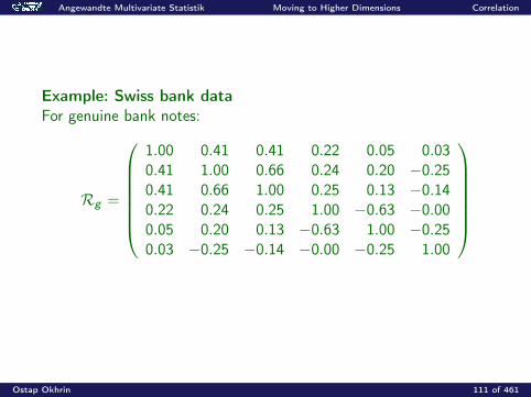
Example: Swiss bank dataFor genuine bank notes:
Rg =
1.00 0.41 0.41 0.22 0.05 0.030.41 1.00 0.66 0.24 0.20 −0.250.41 0.66 1.00 0.25 0.13 −0.140.22 0.24 0.25 1.00 −0.63 −0.000.05 0.20 0.13 −0.63 1.00 −0.250.03 −0.25 −0.14 −0.00 −0.25 1.00
Ostap Okhrin 111 of 461
Angewandte Multivariate Statistik Moving to Higher Dimensions Correlation
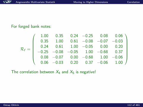
For forged bank notes:
Rf =
1.00 0.35 0.24 −0.25 0.08 0.060.35 1.00 0.61 −0.08 −0.07 −0.030.24 0.61 1.00 −0.05 0.00 0.20−0.25 −0.08 −0.05 1.00 −0.68 0.370.08 −0.07 0.00 −0.68 1.00 −0.060.06 −0.03 0.20 0.37 −0.06 1.00
The correlation between X4 and X5 is negative!
Ostap Okhrin 112 of 461
Angewandte Multivariate Statistik Moving to Higher Dimensions Correlation
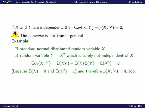
If X and Y are independent, then Cov(X ,Y ) = ρ(X ,Y ) = 0.
The converse is not true in generalExample:
standard normal distributed random variable X
random variable Y = X 2 which is surely not independent of X
Cov(X ,Y ) = E(XY )− E(X )E(Y ) = E(X 3) = 0
(because E(X ) = 0 and E(X 2) = 1) and therefore ρ(X ,Y ) = 0, too.
Ostap Okhrin 113 of 461
Angewandte Multivariate Statistik Moving to Higher Dimensions Correlation
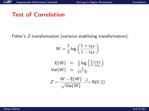
Test of Correlation
Fisher’s Z -transformation (variance stabilizing transformation):
W =12log(1 + rXY1− rXY
)E(W ) ≈ 1
2 log(
1+ρXY1−ρXY
)Var(W ) ≈ 1
(n−3)
Z =W − E(W )√
Var(W )
L−→ N(0, 1)
Ostap Okhrin 114 of 461
Angewandte Multivariate Statistik Moving to Higher Dimensions Correlation
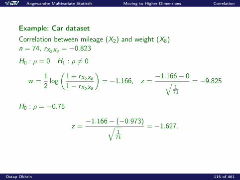
Example: Car datasetCorrelation between mileage (X2) and weight (X8)n = 74, rX2X8 = −0.823
H0 : ρ = 0 H1 : ρ 6= 0
w =12log(1 + rX2X8
1− rX2X8
)= −1.166, z =
−1.166− 0√171
= −9.825
H0 : ρ = −0.75
z =−1.166− (−0.973)√
171
= −1.627.
Ostap Okhrin 115 of 461
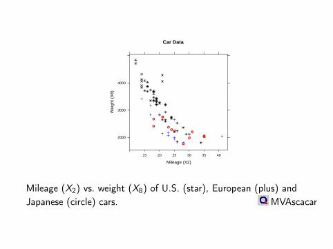
Car Data
Mileage (X2)
Wei
ght (
X8)
2000
3000
4000
15 20 25 30 35 40
Mileage (X2) vs. weight (X8) of U.S. (star), European (plus) andJapanese (circle) cars. MVAscacar
Angewandte Multivariate Statistik Moving to Higher Dimensions Correlation
Summary: Correlation
The correlation is a standardized measure of dependence. The absolute value of the correlation is always less or equal to
one. Correlation measures only linear dependence. There are nonlinear dependencies that have zero correlation. Zero correlation does not imply independence.
Ostap Okhrin 117 of 461
Angewandte Multivariate Statistik Moving to Higher Dimensions Correlation
Summary: Correlation
Independence implies zero correlation. Negative correlation corresponds to downward-sloping
scatterplots. Positive correlation corresponds to upward-sloping scatterplots. Fisher’s Z-transformation helps us in testing hypotheses on
correlation. For small samples, Fisher’s Z-transformation can be improved by
W ∗ = W − 3W+tanh(W )4(n−1) .
Ostap Okhrin 118 of 461
Angewandte Multivariate Statistik Moving to Higher Dimensions Summary Statistics
Summary Statistics
X (n × p) data matrix
X =
x11 · · · x1p...
......
...xn1 . . . xnp
xi = (xi1, · · · , xip)> ∈ Rp: i-th observation of a p-dimensional randomvariable X ∈ Rp
Ostap Okhrin 119 of 461
Angewandte Multivariate Statistik Moving to Higher Dimensions Summary Statistics
Mean
x =
x1...xp
= n−1X>1n
Empirical covariance matrix
S = n−1X>X − x x>
= n−1(X>X − n−1X>1n1>n X ) = n−1X>HX
Centering matrixH = In − n−11n1>n
Ostap Okhrin 120 of 461
Angewandte Multivariate Statistik Moving to Higher Dimensions Summary Statistics
Empirical correlation matrix
R = D−1/2SD−1/2
with D = diag(sXjXj) and D−1/2 = diag(s
−1/2XjXj
) for j = 1, . . . , p.
Ostap Okhrin 121 of 461
Angewandte Multivariate Statistik Moving to Higher Dimensions Summary Statistics
Linear Transformations
A (q × p) matrix
Y = XA> = (y1, . . . , yn)>
y = n−1Y>1n = AxSY = n−1Y>HY = ASXA>
Example:Let x = (1, 2)> and y = 4x , x ∈ R2
Then y = 4x = (4, 8)>.
Ostap Okhrin 122 of 461
Angewandte Multivariate Statistik Moving to Higher Dimensions Summary Statistics
Mahalanobis Transformation
Z = (z1, . . . , zn)>
zi = S−1/2(xi − x), i = 1, . . . , n
SZ = n−1Z>HZ = IpZ = 0
The Mahalanobis transformation leads to standardized uncorrelatedzero mean data matrix Z.
Ostap Okhrin 123 of 461
Angewandte Multivariate Statistik Moving to Higher Dimensions Summary Statistics
Summary: Summary Statistics
The center of gravity of a data matrix is given by its mean vectorx = n−1X>1n.
The dispersion of the observations in a data matrix is given by theempirical covariance matrix S = n−1X>HX .
The empirical correlation matrix is given by R = D−1/2SD−1/2.
Ostap Okhrin 124 of 461
Angewandte Multivariate Statistik Moving to Higher Dimensions Summary Statistics
Summary: Summary Statistics
A linear transformation Y = XA> of a data matrix X has meanAx and empirical covariance ASXA>.
The Mahalanobis transformation is a linear transformationzi = S−1/2(xi − x) which gives a standardized, uncorrelated datamatrix Z.
Ostap Okhrin 125 of 461

Angewandte Multivariate Statistik Moving to Higher Dimensions One-Sample and Two-Sample t-Test
One-sample t-test
We have iid observations x1, . . . , xn.Assume that the observations stem from N(µ, σ2).Then xn ∼ N(µ, σ2/n), i.e.
√n
(xn − µ)
σ∼ N(0, 1).
Ostap Okhrin 126 of 461

Angewandte Multivariate Statistik Moving to Higher Dimensions One-Sample and Two-Sample t-Test
H0 : µ = µ0 H1 : µ 6= µ0Assume that σ2 is known:
√n|xn − µ0|
σ∼ N(0, 1)
Show that P(reject H0|H0 is true) = α.
Ostap Okhrin 127 of 461

Angewandte Multivariate Statistik Moving to Higher Dimensions One-Sample and Two-Sample t-Test
Usually σ2 is not known and we have to estimate it:
σ2n =
1n − 1
n∑i=1
(xi − xn)2.
It can be shown that
√n
(xn − µ)
σn∼ tn−1.
Note: t-distribution tn approaches N(0, 1) as n→∞ (parameter n:degrees of freedom).
Ostap Okhrin 128 of 461

Angewandte Multivariate Statistik Moving to Higher Dimensions One-Sample and Two-Sample t-Test
Test:H0 : E (X ) = µ0 H1 : E (X ) 6= µ0We reject H0 if
√n|xn − µ0|
σn> t1−α/2;n−1.
t1−α/2;n−1: 1− α critical value (i.e. 1− α/2 quantile) of the Student’st-distribution with (n − 1) degrees of freedom
Ostap Okhrin 129 of 461
Angewandte Multivariate Statistik Moving to Higher Dimensions One-Sample and Two-Sample t-Test
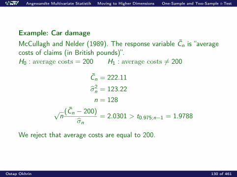
Example: Car damageMcCullagh and Nelder (1989). The response variable Cn is “averagecosts of claims (in British pounds)”.H0 : average costs = 200 H1 : average costs 6= 200
Cn = 222.11
σ2n = 123.22n = 128
√n
(Cn − 200)
σn= 2.0301 > t0.975;n−1 = 1.9788
We reject that average costs are equal to 200.
Ostap Okhrin 130 of 461

Angewandte Multivariate Statistik Moving to Higher Dimensions One-Sample and Two-Sample t-Test
Two-sample t-test
We have two iid samples y11, . . . , y1n and y21, . . . , y2m.Assume that Y11 ∼ N(µ1, σ
2) and Y21 ∼ N(µ2, σ2)
H0 : µ1 = µ2 H1 : µ1 6= µ2Pooled estimate of variance
σ2P =
1m + n − 2
n∑
i=1
(y1i − y1)2 +m∑j=1
(y2j − y2)2
Ostap Okhrin 131 of 461

Angewandte Multivariate Statistik Moving to Higher Dimensions One-Sample and Two-Sample t-Test
Test statistic
T =
√m + n
mn
(y1 − y2)− (µ1 − µ2)
σP∼ tn+m−2
Reject H0 if |T | > t1−α/2;n+m−2.
Ostap Okhrin 132 of 461
Angewandte Multivariate Statistik Moving to Higher Dimensions Linear Model for Two Variables
Linear Model for Two Variables
yi = β0 + β1xi + εi , E (εi ) = 0, Var (εi ) = σ2, i = 1, . . . , nβ0 = intercept, β1 = slope
Estimate (β0, β1) by least squares
(β0, β1) = arg min(β0,β1)
n∑i=1
(yi − β0 − β1xi )2
β1 =sXYsXX
=Cov(X ,Y )
Var(X )
β0 = y − β1x
Ostap Okhrin 133 of 461
Price (X2)
Sal
es (
X1)
Pullovers Data
8012
016
020
024
0
80 90 100 110 120
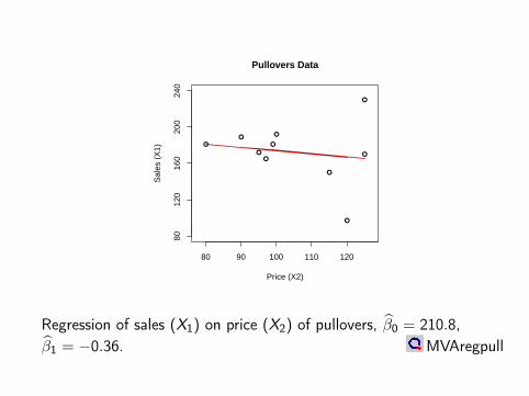
Regression of sales (X1) on price (X2) of pullovers, β0 = 210.8,β1 = −0.36. MVAregpull
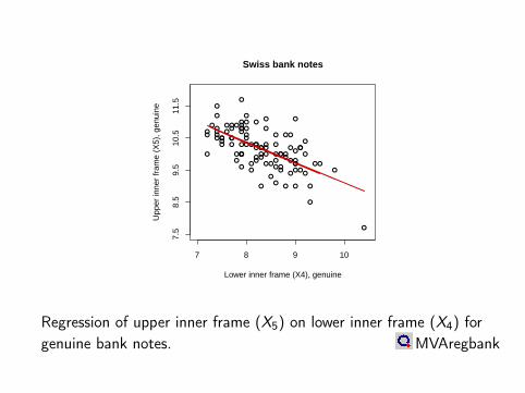
Lower inner frame (X4), genuine
Upp
er in
ner
fram
e (X
5), g
enui
ne
7.5
8.5
9.5
10.5
11.5
7 8 9 10
Swiss bank notes
Regression of upper inner frame (X5) on lower inner frame (X4) forgenuine bank notes. MVAregbank
Angewandte Multivariate Statistik Moving to Higher Dimensions Linear Model for Two Variables
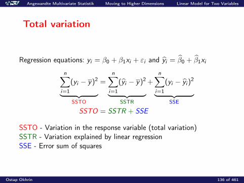
Total variation
Regression equations: yi = β0 + β1xi + εi and yi = β0 + β1xi
n∑i=1
(yi − y)2
︸ ︷︷ ︸SSTO
=n∑
i=1
(yi − y)2
︸ ︷︷ ︸SSTR
+n∑
i=1
(yi − yi )2
︸ ︷︷ ︸SSE
SSTO = SSTR + SSE
SSTO - Variation in the response variable (total variation)SSTR - Variation explained by linear regressionSSE - Error sum of squares
Ostap Okhrin 136 of 461
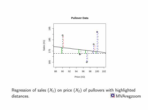
88 90 92 94 96 98 100 102
165
175
185
195
Price (X2)
Sal
es (
X1)
Pullover Data
Regression of sales (X1) on price (X2) of pullovers with highlighteddistances. MVAregzoom
Angewandte Multivariate Statistik Moving to Higher Dimensions Linear Model for Two Variables
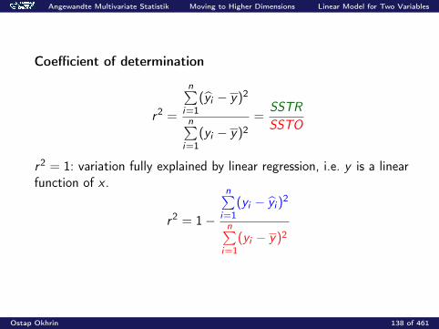
Coefficient of determination
r2 =
n∑i=1
(yi − y)2
n∑i=1
(yi − y)2=
SSTR
SSTO
r2 = 1: variation fully explained by linear regression, i.e. y is a linearfunction of x .
r2 = 1−
n∑i=1
(yi − yi )2
n∑i=1
(yi − y)2
Ostap Okhrin 138 of 461
Angewandte Multivariate Statistik Moving to Higher Dimensions Linear Model for Two Variables
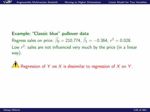
Example: “Classic blue” pullover dataRegress sales on price: β0 = 210.774, β1 = −0.364, r2 = 0.028.Low r2: sales are not influenced very much by the price (in a linearway).
Regression of Y on X is dissimilar to regression of X on Y .
Ostap Okhrin 139 of 461

Angewandte Multivariate Statistik Moving to Higher Dimensions Linear Model for Two Variables
t-Test for β1
H0 : β1 = 0 (ρXY = 0) H1 : β1 6= 0
Var(β1) =σ2
(n · sXX ), SE (β1) =
σ
(n · sXX )1/2 , t =β1
SE (β1)
t1−α/2;n−2: 1− α critical value (i.e. 1− α/2 quantile) of the Student’st-distribution with (n − 2) degrees of freedom
Do not reject H0 if |t| ≤ t1−α/2;n−2
Ostap Okhrin 140 of 461
Angewandte Multivariate Statistik Moving to Higher Dimensions Linear Model for Two Variables
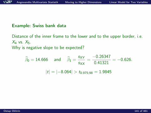
Example: Swiss bank data
Distance of the inner frame to the lower and to the upper border, i.e.X4 vs. X5.Why is negative slope to be expected?
β0 = 14.666 and β1 =sXYsXX
=−0.263470.41321
= −0.626.
|t| = |−8.064| > t0.975;98 = 1.9845
Ostap Okhrin 141 of 461
Angewandte Multivariate Statistik Moving to Higher Dimensions Linear Model for Two Variables
Summary: Linear Regression
The linear regression y = β0 + β1x + ε models a linear relationbetween two one-dimensional variables.
The sign of the slope β1 is the same as that of the covariance andthe correlation of x and y .
A linear regression predicts values of Y given a possibleobservation x of X .
Ostap Okhrin 142 of 461
Angewandte Multivariate Statistik Moving to Higher Dimensions Linear Model for Two Variables
Summary: Linear Regression
The coefficient of determination r2 measures the amount ofvariation in Y which is explained by a linear regression on X .
If the coefficient of determination is r2 = 1, then all points lie onone line.
The regression line of X on Y and the regression line of Y on Xare in general different.
Ostap Okhrin 143 of 461
Angewandte Multivariate Statistik Moving to Higher Dimensions Linear Model for Two Variables
Summary: Linear Regression
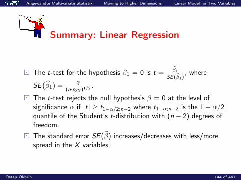
The t-test for the hypothesis β1 = 0 is t = β1SE(β1)
, where
SE (β1) = σ(n·sXX )1/2
.
The t-test rejects the null hypothesis β = 0 at the level ofsignificance α if |t| ≥ t1−α/2;n−2 where t1−α;n−2 is the 1− α/2quantile of the Student’s t-distribution with (n − 2) degrees offreedom.
The standard error SE (β) increases/decreases with less/morespread in the X variables.
Ostap Okhrin 144 of 461
Angewandte Multivariate Statistik Moving to Higher Dimensions Simple Analysis of Variance
Simple Analysis of Variance (ANOVA)
Assumptions
Average values of the response variable y are induced by onesimple factor
Factor takes on p values For each factor level, we have m = n/p observations All observations are independent
Ostap Okhrin 145 of 461
Angewandte Multivariate Statistik Moving to Higher Dimensions Simple Analysis of Variance
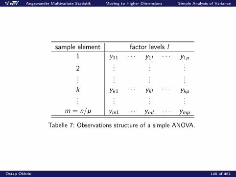
sample element factor levels l1 y11 · · · y1l · · · y1p
2...
......
......
......
k yk1 · · · ykl · · · ykp...
......
...m = n/p ym1 · · · yml · · · ymp
Tabelle 7: Observations structure of a simple ANOVA.
Ostap Okhrin 146 of 461
Angewandte Multivariate Statistik Moving to Higher Dimensions Simple Analysis of Variance
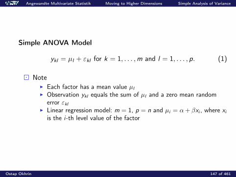
Simple ANOVA Model
ykl = µl + εkl for k = 1, . . . ,m and l = 1, . . . , p. (1)
NoteI Each factor has a mean value µl
I Observation ykl equals the sum of µl and a zero mean randomerror εkl
I Linear regression model: m = 1, p = n and µi = α+ βxi , where xiis the i-th level value of the factor
Ostap Okhrin 147 of 461

Angewandte Multivariate Statistik Moving to Higher Dimensions Simple Analysis of Variance
Example: “Classic blue” pullover data
Analyse the effect of three marketing strategies:1. Advertisement in local newspapers2. Presence of sales assistant3. Luxury presentation in shop windows
p = 3 factors, 10 different shops and n = mp = 30 observations
Ostap Okhrin 148 of 461

Angewandte Multivariate Statistik Moving to Higher Dimensions Simple Analysis of Variance
shop marketing strategyk factor l
1 2 31 9 10 182 11 15 143 10 11 174 12 15 95 7 15 146 11 13 177 12 7 168 10 15 149 11 13 1710 13 10 15
Tabelle 8: Pullover sales as function of marketing strategy.
Ostap Okhrin 149 of 461

Angewandte Multivariate Statistik Moving to Higher Dimensions Simple Analysis of Variance
Do all three strategies have the same mean effect?
Test
H0 : µl = µ for l = 1, . . . , p vs. H1 : µl 6= µl ′ for some l and l ′
Alternative: one marketing strategy is better than the others
Ostap Okhrin 150 of 461
Angewandte Multivariate Statistik Moving to Higher Dimensions Simple Analysis of Variance
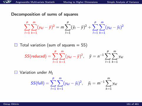
Decomposition of sums of squares
p∑l=1
m∑k=1
(ykl − y)2 = m
p∑l=1
(yl − y)2 +
p∑l=1
m∑k=1
(ykl − yl)2
Total variation (sum of squares = SS)
SS(reduced) =
p∑l=1
m∑k=1
(ykl − y)2, y = n−1p∑
l=1
m∑k=1
ykl
Variation under H1
SS(full) =
p∑l=1
m∑k=1
(ykl − yl)2, yl = m−1
m∑k=1
ykl
Ostap Okhrin 151 of 461
Angewandte Multivariate Statistik Moving to Higher Dimensions Simple Analysis of Variance
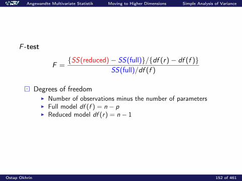
F -test
F =SS(reduced)− SS(full)/df (r)− df (f )
SS(full)/df (f )
Degrees of freedomI Number of observations minus the number of parametersI Full model df (f ) = n − pI Reduced model df (r) = n − 1
Ostap Okhrin 152 of 461
Angewandte Multivariate Statistik Moving to Higher Dimensions Simple Analysis of Variance
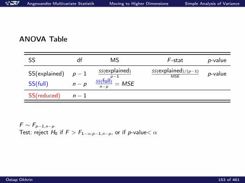
ANOVA Table
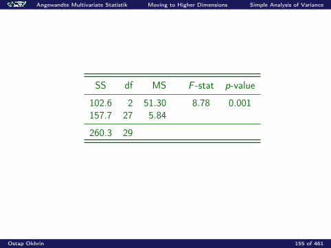
SS df MS F -stat p-value
SS(explained) p − 1 SS(explained)
p−1SS(explained)/(p−1)
MSEp-value
SS(full) n − p SS(full)n−p
= MSE
SS(reduced) n − 1
F ∼ Fp−1,n−p
Test: reject H0 if F > F1−α;p−1,n−p, or if p-value< α
Ostap Okhrin 153 of 461
Angewandte Multivariate Statistik Moving to Higher Dimensions Simple Analysis of Variance
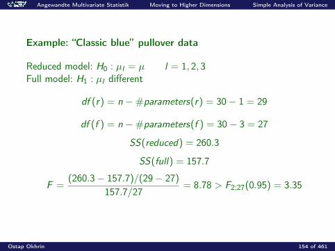
Example: “Classic blue” pullover data
Reduced model: H0 : µl = µ l = 1, 2, 3Full model: H1 : µl different
df (r) = n −#parameters(r) = 30− 1 = 29
df (f ) = n −#parameters(f ) = 30− 3 = 27
SS(reduced) = 260.3
SS(full) = 157.7
F =(260.3− 157.7)/(29− 27)
157.7/27= 8.78 > F2;27(0.95) = 3.35
Ostap Okhrin 154 of 461
Angewandte Multivariate Statistik Moving to Higher Dimensions Simple Analysis of Variance
SS df MS F -stat p-value
102.6 2 51.30 8.78 0.001157.7 27 5.84
260.3 29
Ostap Okhrin 155 of 461
Angewandte Multivariate Statistik Moving to Higher Dimensions Simple Analysis of Variance
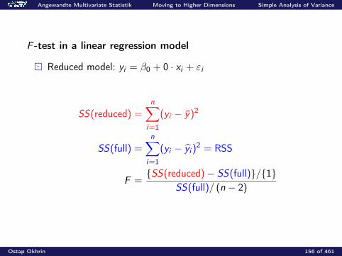
F -test in a linear regression model
Reduced model: yi = β0 + 0 · xi + εi
SS(reduced) =n∑
i=1
(yi − y)2
SS(full) =n∑
i=1
(yi − yi )2 = RSS
F =SS(reduced)− SS(full)/1
SS(full)/ (n − 2)
Ostap Okhrin 156 of 461
Angewandte Multivariate Statistik Moving to Higher Dimensions Simple Analysis of Variance
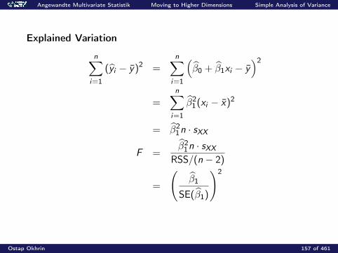
Explained Variation
n∑i=1
(yi − y)2 =n∑
i=1
(β0 + β1xi − y
)2
=n∑
i=1
β21(xi − x)2
= β21n · sXX
F =β2
1n · sXXRSS/(n − 2)
=
(β1
SE(β1)
)2
Ostap Okhrin 157 of 461
Angewandte Multivariate Statistik Moving to Higher Dimensions Simple Analysis of Variance
Summary: ANOVA
Simple ANOVA models an output Y as a function of one factor. The reduced model is the hypothesis of equal means. The full model is the alternative hypothesis of different means. The F -test is based on a comparison of the sum of squares under
the full and the reduced models.
Ostap Okhrin 158 of 461
Angewandte Multivariate Statistik Moving to Higher Dimensions Simple Analysis of Variance
Summary: ANOVA
The degrees of freedom are calculated as the number ofobservations minus the number of parameters.
The F -statistic is
F =SS(reduced)− SS(full)/df (r)− df (f )
SS(full)/df (f ).
Reject the null if the F -statistic is larger than the(1− α)-quantile of the Fdf (r)−df (f ),df (f ) distribution.
The F -test statistic for the slope of the linear regression modelyi = β0 + β1xi + εi is the square of the t-test statistic.
Ostap Okhrin 159 of 461
Angewandte Multivariate Statistik Moving to Higher Dimensions The Multiple Linear Model
Multiple Linear Model
y(n × 1), X (n × p), β = (β1, . . . , βp)
Approximate y by a linear combination y of columns of XFind β such that y = X β is the best fit of y = Xβ + ε (errors ε)
β = argminβ
(y −Xβ)>(y −Xβ)
= argminβ
n∑i=1
(yi − x>i β)2 =(X>X
)−1X>y ,
if X>X is of full rank.
Ostap Okhrin 160 of 461
Angewandte Multivariate Statistik Moving to Higher Dimensions The Multiple Linear Model
Linear Model with Intercept
yi = β0 + β1xi1 + . . .+ βpxip + εi i = 1, . . . , n
can be written asy = X ∗β∗ + ε
whereX ∗ = (1n X )
β∗ =
(β0β
)= (X ∗>X ∗)−1X ∗>y
Ostap Okhrin 161 of 461

Angewandte Multivariate Statistik Moving to Higher Dimensions The Multiple Linear Model
Example: “Classic blue” pullover dataApproximate the sales as a linear function of the three other variables:price (X2), advertisement (X3) and presence of sales assistants (X4)Adding a column of ones to the data (in order to estimate also theintercept β0) leads to
β0 = 65.670, β1 = −0.216, β2 = 0.485, β3 = 0.844.
Coefficient of determination: r2 = 0.907
Ostap Okhrin 162 of 461
Angewandte Multivariate Statistik Moving to Higher Dimensions The Multiple Linear Model
Remark:The coefficient of determination is influenced by the number ofregressors.For a given sample size n, the r2 value will increase by adding moreregressors into the linear model.A corrected coefficient of determination for p regressors anda constant intercept:
r2adj = r2 − p(1− r2)
n − (p + 1)
Ostap Okhrin 163 of 461
Angewandte Multivariate Statistik Moving to Higher Dimensions The Multiple Linear Model
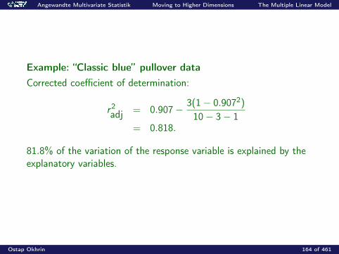
Example: “Classic blue” pullover dataCorrected coefficient of determination:
r2adj = 0.907− 3(1− 0.9072)
10− 3− 1= 0.818.
81.8% of the variation of the response variable is explained by theexplanatory variables.
Ostap Okhrin 164 of 461
Angewandte Multivariate Statistik Moving to Higher Dimensions The Multiple Linear Model
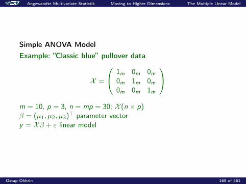
Simple ANOVA ModelExample: “Classic blue” pullover data
X =
1m 0m 0m0m 1m 0m0m 0m 1m
m = 10, p = 3, n = mp = 30; X (n × p)β = (µ1, µ2, µ3)> parameter vectory = Xβ + ε linear model
Ostap Okhrin 165 of 461
Angewandte Multivariate Statistik Moving to Higher Dimensions The Multiple Linear Model
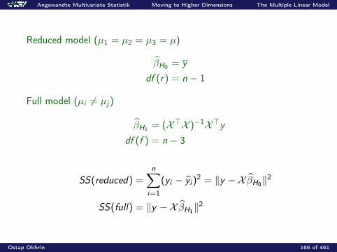
Reduced model (µ1 = µ2 = µ3 = µ)
βH0 = y
df (r) = n − 1
Full model (µi 6= µj)
βH1 = (X>X )−1X>ydf (f ) = n − 3
SS(reduced) =n∑
i=1
(yi − yi )2 = ‖y −X βH0‖2
SS(full) = ‖y −X βH1‖2
Ostap Okhrin 166 of 461
Angewandte Multivariate Statistik Moving to Higher Dimensions The Multiple Linear Model
Simple ANOVA Model - F−test
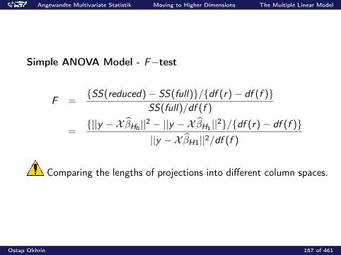
F =SS(reduced)− SS(full)/df (r)− df (f )
SS(full)/df (f )
=||y −X βH0 ||2 − ||y −X βH1 ||2/df (r)− df (f )
||y −X βH1||2/df (f )
Comparing the lengths of projections into different column spaces.
Ostap Okhrin 167 of 461
Angewandte Multivariate Statistik Moving to Higher Dimensions The Multiple Linear Model
Summary: Multiple Linear Model
The relation y = Xβ + ε models a linear relation betweena one-dimensional variable Y and a p-dimensional variable X . Pygives the best linear regression fit of the vector y onto C (X ). Theleast squares parameter estimator is β = (X>X )−1X>y .
The simple ANOVA model can be written as a linear model.
Ostap Okhrin 168 of 461
Angewandte Multivariate Statistik Moving to Higher Dimensions The Multiple Linear Model
Summary: Multiple Linear Model
The ANOVA model can be tested by comparing the length of theprojection vectors.
The test statistic of the F -test can be written as
||y −X βH0 ||2 − ||y −X βH1 ||2/df (r)− df (f )||y −X βH1 ||2/df (f )
.
The adjusted coefficient of determination is
r2adj = r2 − p(1− r2)
n − (p + 1).
Ostap Okhrin 169 of 461
Angewandte Multivariate Statistik Multivariate Distributions Multivariate Distributions
Multivariate Distributions
Random vector X ∈ Rp
(Multivariate) distribution function is
F (x) = P(X ≤ x) = P(X1 ≤ x1,X2 ≤ x2, . . . ,Xp ≤ xp)
f (x) denotes density of X , i.e.
F (x) =
∫ x
−∞f (u)du
∫ ∞−∞
f (u) du = 1
PX ∈ (a, b) =
b∫a
f (x)dx
Ostap Okhrin 170 of 461

Angewandte Multivariate Statistik Multivariate Distributions Multivariate Distributions
X = (X1,X2)>, X1 ∈ Rk X2 ∈ Rp−k
Marginal density of X1 is
fX1(x1) =
∫ ∞−∞
f (x1, x2)dx2
Conditional density of X2 (conditioned on X1 = x1)
fX2|X1=x1(x2) = f (x1, x2)/fX1(x1)
Ostap Okhrin 171 of 461
Angewandte Multivariate Statistik Multivariate Distributions Multivariate Distributions
Example
f (x1, x2) =
12x1 + 3
2x2 0 ≤ x1, x2 ≤ 1,0 otherwise.
f (x1, x2) is a density since∫f (x1, x2)dx1x2 =
12
[x212
]1
0+
32
[x222
]1
0=
14
+34
= 1.
Ostap Okhrin 172 of 461

Angewandte Multivariate Statistik Multivariate Distributions Multivariate Distributions
The marginal densities
fX1(x1) =
∫f (x1, x2)dx2 =
∫ 1
0
(12x1 +
32x2
)dx2 =
12x1 +
34
;
fX2(x2) =
∫f (x1, x2)dx1 =
∫ 1
0
(12x1 +
32x2
)dx1 =
32x2 +
14·
The conditional densities
f (x2 | x1) =12x1 + 3
2x212x1 + 3
4and f (x1 | x2) =
12x1 + 3
2x232x2 + 1
4·
These conditional pdf’s are nonlinear in x1 and x2 although the jointpdf has a simple (linear) structure.
Ostap Okhrin 173 of 461
Angewandte Multivariate Statistik Multivariate Distributions Multivariate Distributions
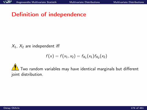
Definition of independence
X1, X2 are independent iff
f (x) = f (x1, x2) = fX1(x1)fX2(x2)
Two random variables may have identical marginals but differentjoint distribution.
Ostap Okhrin 174 of 461

Angewandte Multivariate Statistik Multivariate Distributions Multivariate Distributions
Example
f (x1, x2) = 1, 0 < x1, x2 < 1,
f (x1, x2) = 1 + α(2x1 − 1)(2x2 − 1), 0 < x1, x2 < 1, −1 ≤ α ≤ 1.
fX1(x1) = 1, fX2(x2) = 1.∫ 1
01 + α(2x1 − 1)(2x2 − 1)dx2 = 1 + α(2x1 − 1)[x2
2 − x2]10 = 1.
Ostap Okhrin 175 of 461
7 8 9 10 11
0.0
0.1
0.2
0.3
0.4
0.5
Swiss bank notes
Lower Inner Frame (X4)
Den
sity
7 8 9 10 11 12
0.0
0.1
0.2
0.3
0.4
0.5
0.6
Swiss bank notes
Upper Inner Frame (X5)D
ensi
ty
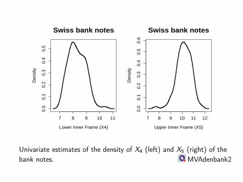
Univariate estimates of the density of X4 (left) and X5 (right) of thebank notes. MVAdenbank2
68
1012
14
810
12
0
0.05
0.1
0.15
0.2
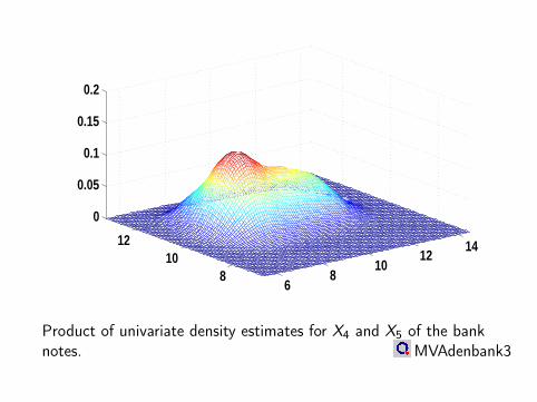
Product of univariate density estimates for X4 and X5 of the banknotes. MVAdenbank3
5
10
15 510
15
0
0.05
0.1
0.15
0.2
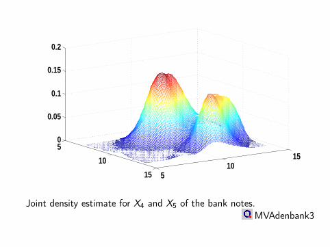
Joint density estimate for X4 and X5 of the bank notes.MVAdenbank3
Angewandte Multivariate Statistik Multivariate Distributions Multivariate Distributions
Summary: Distributions
The cumulative distribution function (cdf) is F (x) = P(X < x). If a probability density function (pdf) f exists then
F (x) =
∫ x
−∞f (u)du.
Let X = (X1,X2)> be partitioned in subvectors X1 and X2 withjoint cdf F . Then FX1(x1) = P(X1 ≤ x1) is the marginal cdf of
X1. The marginal pdf of X1 is fX1(x1) =
∫ ∞−∞
f (x1, x2)dx2.
Ostap Okhrin 179 of 461

Angewandte Multivariate Statistik Multivariate Distributions Multivariate Distributions
Summary: Distributions
Different joint pdf’s may have the same marginal pdf’s.
The conditional pdf of X2 given X1 = x1 is f (x2 | x1) =f (x1, x2)
fX1(x1)·
Two random variables X1,X2 are called independent ifff (x1, x2) = fX1(x1)fX2(x2). This is equivalent tof (x2 | x1) = fX2(x2).
Ostap Okhrin 180 of 461
Angewandte Multivariate Statistik Multivariate Distributions Moments and Characteristic Functions
Moments and Characteristic Functions
EX ∈ Rp denotes the p-dimensional vector of expected values of therandom vector X
EX =
EX1...
EXp
=
∫xf (x)dx =
∫x1f (x)dx
...∫xpf (x)dx
= µ.
The properties of the expected value follow from the properties of theintegral:
E (αX + βY ) = αEX + β EY
Ostap Okhrin 181 of 461
Angewandte Multivariate Statistik Multivariate Distributions Moments and Characteristic Functions
If X and Y are independent then
E(XY>) =
∫xy>f (x , y)dxdy
=
∫xf (x)dx
∫y>f (y)dy = EX EY>
Definition of the covariance matrix (Σ)
Σ = Var(X ) = E(X − µ)(X − µ)>
We say that a random vector X has a distribution with the vector ofexpected values µ and the covariance matrix Σ,
X ∼ (µ,Σ)
Ostap Okhrin 182 of 461
Angewandte Multivariate Statistik Multivariate Distributions Moments and Characteristic Functions
Properties of the Covariance Matrix
Elements of Σ are variances and covariances of the components of therandom vector X :
Σ = (σXiXj)
σXiXj= Cov(Xi ,Xj)
σXiXi= Var(Xi )
Computational formula: Σ = E(XX>)− µµ>Covariance matrix is positive semidefinite, Σ ≥ 0(variance a>Σa of any linear combination a>X cannot be negative).
Ostap Okhrin 183 of 461
Angewandte Multivariate Statistik Multivariate Distributions Moments and Characteristic Functions
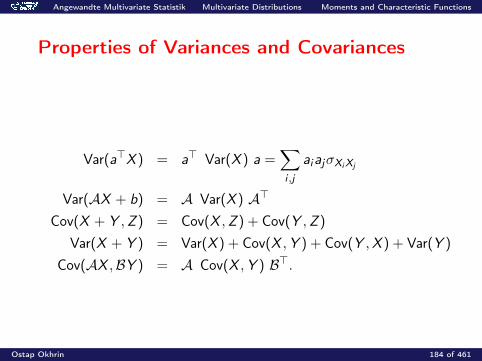
Properties of Variances and Covariances
Var(a>X ) = a> Var(X ) a =∑i ,j
aiajσXiXj
Var(AX + b) = A Var(X ) A>
Cov(X + Y ,Z ) = Cov(X ,Z ) + Cov(Y ,Z )
Var(X + Y ) = Var(X ) + Cov(X ,Y ) + Cov(Y ,X ) + Var(Y )
Cov(AX ,BY ) = A Cov(X ,Y ) B>.
Ostap Okhrin 184 of 461
Angewandte Multivariate Statistik Multivariate Distributions Moments and Characteristic Functions
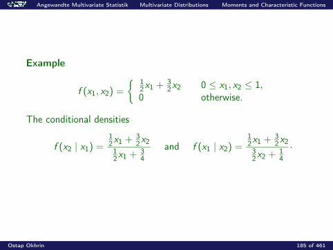
Example
f (x1, x2) =
12x1 + 3
2x2 0 ≤ x1, x2 ≤ 1,0 otherwise.
The conditional densities
f (x2 | x1) =12x1 + 3
2x212x1 + 3
4and f (x1 | x2) =
12x1 + 3
2x232x2 + 1
4·
Ostap Okhrin 185 of 461

Angewandte Multivariate Statistik Multivariate Distributions Moments and Characteristic Functions
µ1 =
∫ ∫x1f (x1, x2)dx1dx2 =
∫ 1
0
∫ 1
0x1
(12x1 +
32x2
)dx1dx2
=
∫ 1
0x1
(12x1 +
34
)dx1 =
12
[x313
]1
0+
34
[x212
]1
0
=16
+38
=4 + 924
=1324
,
µ2 =
∫ ∫x2f (x1, x2)dx1dx2 =
∫ 1
0
∫ 1
0x2
(12x1 +
32x2
)dx1dx2
=
∫ 1
0x2
(14
+32x2
)dx2 =
14
[x222
]1
0+
32
[x323
]1
0
=18
+12
=1 + 48
=58·
Ostap Okhrin 186 of 461
Angewandte Multivariate Statistik Multivariate Distributions Moments and Characteristic Functions
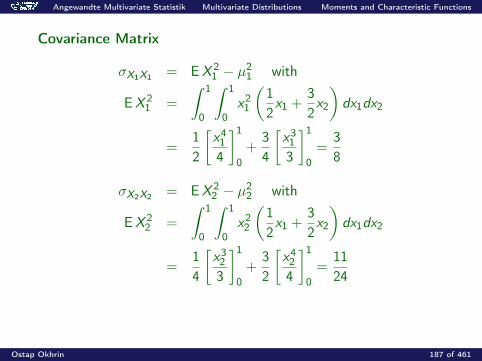
Covariance Matrix
σX1X1 = EX 21 − µ2
1 with
EX 21 =
∫ 1
0
∫ 1
0x21
(12x1 +
32x2
)dx1dx2
=12
[x414
]1
0+
34
[x313
]1
0=
38
σX2X2 = EX 22 − µ2
2 with
EX 22 =
∫ 1
0
∫ 1
0x22
(12x1 +
32x2
)dx1dx2
=14
[x323
]1
0+
32
[x424
]1
0=
1124
Ostap Okhrin 187 of 461
Angewandte Multivariate Statistik Multivariate Distributions Moments and Characteristic Functions
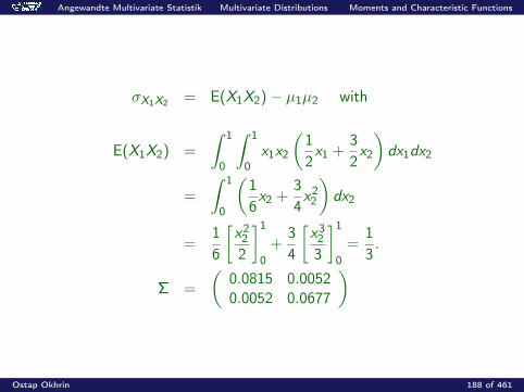
σX1X2 = E(X1X2)− µ1µ2 with
E(X1X2) =
∫ 1
0
∫ 1
0x1x2
(12x1 +
32x2
)dx1dx2
=
∫ 1
0
(16x2 +
34x22
)dx2
=16
[x222
]1
0+
34
[x323
]1
0=
13.
Σ =
(0.0815 0.00520.0052 0.0677
)
Ostap Okhrin 188 of 461
Angewandte Multivariate Statistik Multivariate Distributions Moments and Characteristic Functions
Conditional Expectations
Random vector X = (X1,X2)>, X1 ∈ Rk X2 ∈ Rp−k
Conditional expectation of X2, given X1 = x1:
E(X2 | x1) =
∫x2f (x2 | x1) dx2
and conditional expectation of X1, given X2 = x2:
E(X1 | x2) =
∫x1f (x1 | x2) dx1
The conditional expectation E(X2 | x1) is a function of x1.Typical example of this setup is a simple linear regression, whereE(Y | X = x) = Xβ.
Ostap Okhrin 189 of 461

Angewandte Multivariate Statistik Multivariate Distributions Moments and Characteristic Functions
Error term in approximation:
U = X2 − E(X2 | X1)
(1) E(U) = 0(2) E(X2|X1) is the best approximation of X2 by a function h(X1) of
X1 in the sense of mean squared error (MSE) whenMSE (h) = E[X2 − h(X1)> X2 − h(X1)] andh : Rk −→ Rp−k .
Ostap Okhrin 190 of 461
Angewandte Multivariate Statistik Multivariate Distributions Moments and Characteristic Functions
Summary: Moments
The expectation of a random vector X is µ =∫xf (x) dx , the
covariance matrix Σ = Var(X ) = E(X − µ)(X − µ)>. We denoteX ∼ (µ,Σ).
Expectations are linear, i.e., E(αX + βY ) = αEX + β EY . IfX ,Y are independent then E(XY>) = EX EY>.
Ostap Okhrin 191 of 461
Angewandte Multivariate Statistik Multivariate Distributions Moments and Characteristic Functions
Summary: Moments
The covariance between two random vectors X ,Y is ΣXY =Cov(X ,Y ) = E(X − EX )(Y − EY )> = E(XY>)− EX EY>. IfX ,Y are independent then Cov(X ,Y ) = 0.
The conditional expectation E(X2|X1) is the MSE bestapproximation of X2 by a function of X1.
Ostap Okhrin 192 of 461
Angewandte Multivariate Statistik Multivariate Distributions Moments and Characteristic Functions
Characteristic Functions
The characteristic function (cf) of a random vector X ∈ Rp is definedas
ϕX (t) = E(e it>X ) =
∫e it>x f (x) dx , t ∈ Rp,
where i is the complex unit: i2 = −1.
Ostap Okhrin 193 of 461

Angewandte Multivariate Statistik Multivariate Distributions Moments and Characteristic Functions
Properties of cf: ϕX (0) = 1, |ϕX (t)| ≤ 1
if ϕ is absolutely integrable (∫ ∞−∞|ϕ(x)|dx exists and is finite)
thenf (x) =
1(2π)p
∫ ∞−∞
e−it>xϕX (t) dt.
if X = (X1,X2, . . . ,Xp)> then for t = (t1, t2, . . . , tp)> :
ϕX1(t1) = ϕX (t1, 0, . . . , 0), . . . , ϕXp(tp) = ϕX (0, . . . , 0, tp).
Ostap Okhrin 194 of 461
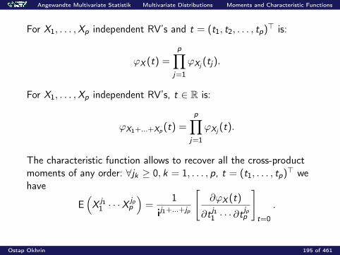
Angewandte Multivariate Statistik Multivariate Distributions Moments and Characteristic Functions
For X1, . . . ,Xp independent RV’s and t = (t1, t2, . . . , tp)> is:
ϕX (t) =
p∏j=1
ϕXj(tj).
For X1, . . . ,Xp independent RV’s, t ∈ R is:
ϕX1+...+Xp(t) =
p∏j=1
ϕXj(t).
The characteristic function allows to recover all the cross-productmoments of any order: ∀jk ≥ 0, k = 1, . . . , p, t = (t1, . . . , tp)> wehave
E(X j1
1 · · ·Xjpp
)=
1ij1+...+jp
[∂ϕX (t)
∂t j11 · · · ∂tjpp
]t=0
.
Ostap Okhrin 195 of 461
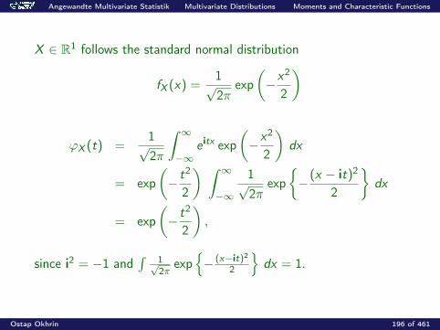
Angewandte Multivariate Statistik Multivariate Distributions Moments and Characteristic Functions
X ∈ R1 follows the standard normal distribution
fX (x) =1√2π
exp(−x2
2
)
ϕX (t) =1√2π
∫ ∞−∞
e itx exp(−x2
2
)dx
= exp(− t2
2
) ∫ ∞−∞
1√2π
exp−(x − it)2
2
dx
= exp(− t2
2
),
since i2 = −1 and∫ 1√
2πexp− (x−it)2
2
dx = 1.
Ostap Okhrin 196 of 461
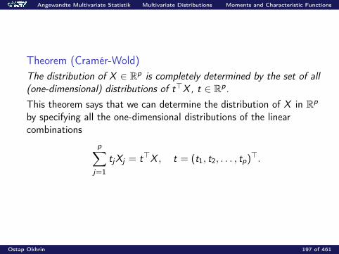
Angewandte Multivariate Statistik Multivariate Distributions Moments and Characteristic Functions
Theorem (Cramér-Wold)The distribution of X ∈ Rp is completely determined by the set of all(one-dimensional) distributions of t>X , t ∈ Rp.This theorem says that we can determine the distribution of X in Rp
by specifying all the one-dimensional distributions of the linearcombinations
p∑j=1
tjXj = t>X , t = (t1, t2, . . . , tp)>.
Ostap Okhrin 197 of 461
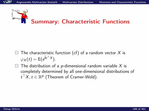
Angewandte Multivariate Statistik Multivariate Distributions Moments and Characteristic Functions
Summary: Characteristic Functions
The characteristic function (cf) of a random vector X isϕX (t) = E(eit>X ).
The distribution of a p-dimensional random variable X iscompletely determined by all one-dimensional distributions oft>X , t ∈ Rp (Theorem of Cramer-Wold).
Ostap Okhrin 198 of 461
Angewandte Multivariate Statistik Multivariate Distributions Moments and Characteristic Functions
Cumulants
For a random variable X with density f and finite moments of order kthe characteristic function ϕX (t) = E(e itX ) has a derivative[
∂ϕ(j)X
∂t
]t=0
= κj , j = 1, . . . , k.
The values κj are called cumulants or semi-invariants since κj does notchange (for j > 1) under a shift transformation X 7→ X + a. Thecumulants are natural parameters for dimension reduction methods, inparticular the Projection Pursuit method.
Ostap Okhrin 199 of 461

Angewandte Multivariate Statistik Multivariate Distributions Moments and Characteristic Functions
The relation between the first k moments m1, . . . ,mk and thecumulants is given by
κk = (−1)k−1
∣∣∣∣∣∣∣∣∣∣∣∣∣
m1 1 . . . 0
m2
(10
)m1 . . .
......
. . ....
mk
(k − 10
)mk−1 . . .
(k − 1k − 2
)m1
∣∣∣∣∣∣∣∣∣∣∣∣∣.
Ostap Okhrin 200 of 461

Angewandte Multivariate Statistik Multivariate Distributions Moments and Characteristic Functions
Suppose that k = 1, thenκ1 = m1.
For k = 2 we obtain
κ2 = −
∣∣∣∣∣∣m1 1
m2
(10
)m1
∣∣∣∣∣∣ = m2 −m21
Ostap Okhrin 201 of 461

Angewandte Multivariate Statistik Multivariate Distributions Moments and Characteristic Functions
For k = 3 we have to calculate
κ3 = −
∣∣∣∣∣∣m1 1 0m2 m1 1m3 m2 2m1
∣∣∣∣∣∣Calculating this determinant we arrive at:
κ3 = m1
∣∣∣∣ m1 1m2 2m1
∣∣∣∣−m2
∣∣∣∣ 1 0m2 2m1
∣∣∣∣+ m3
∣∣∣∣ 1 0m1 1
∣∣∣∣= m1(2m2
1 −m2)−m2(2m1) + m3
= m3 − 3m1m2 + 2m31.
In a similar way one calculates
κ4 = m4 − 4m3m1 − 3m22 + 12m2m
21 − 6m4
1.
Ostap Okhrin 202 of 461
Angewandte Multivariate Statistik Multivariate Distributions Moments and Characteristic Functions
In a similar fashion we find the moments from the cumulants:
m1 = κ1
m2 = κ2 + κ21
m3 = κ3 + 3κ2κ1 + κ31
m4 = κ4 + 4κ3κ1 + 3κ22 + 6κ2κ
21 + κ4
1
A very simple relationship can be observed between the semi-invariantsand the central moments µk = E(X − µ)k , where µ = m1 as definedbefore. We have, in fact, κ2 = µ2, κ3 = µ3, κ4 = µ4 − 3µ2
2.
Ostap Okhrin 203 of 461
Angewandte Multivariate Statistik Multivariate Distributions Moments and Characteristic Functions
Skewness γ3 and kurtosis γ4 are defined as:
γ3 = E(X − µ)3/σ3
γ4 = E(X − µ)4/σ4
The skewness and kurtosis determine the shape of one-dimensionaldistributions. The skewness of a normal distribution is 0 and thekurtosis equals 3. The relation of these parameters to the cumulants isgiven by:
γ3 =κ3
κ3/22
γ4 =κ4
κ22
Ostap Okhrin 204 of 461
Angewandte Multivariate Statistik Multivariate Distributions Transformations
Transformations
Suppose X ∼ fX . What is the pdf of Y = 3X?
X = u(Y )
one-to-one transformation u: Rp → Rp
Jacobian:
J =
(∂xi∂yj
)=
∂ui (y)
∂yj
fY (y) = abs(|J |)fXu(y)
Ostap Okhrin 205 of 461
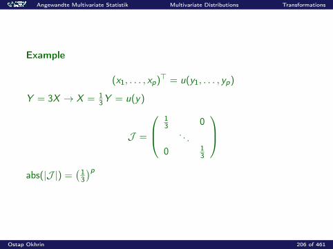
Angewandte Multivariate Statistik Multivariate Distributions Transformations
Example
(x1, . . . , xp)> = u(y1, . . . , yp)
Y = 3X → X = 13Y = u(y)
J =
13 0
. . .0 1
3
abs(|J |) =
(13
)p
Ostap Okhrin 206 of 461

Angewandte Multivariate Statistik Multivariate Distributions Transformations
Y = AX + b, A nonsingular
X = A−1(Y − b)
J = A−1
fY (y) = abs(|A|−1)fXA−1(y − b)
Ostap Okhrin 207 of 461
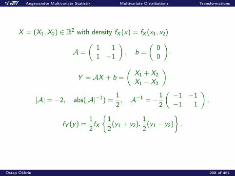
Angewandte Multivariate Statistik Multivariate Distributions Transformations
X = (X1,X2) ∈ R2 with density fX (x) = fX (x1, x2)
A =
(1 11 −1
), b =
(00
).
Y = AX + b =
(X1 + X2X1 − X2
)|A| = −2, abs(|A|−1) =
12, A−1 = −1
2
(−1 −1−1 1
).
fY (y) =12fX
12
(y1 + y2),12
(y1 − y2)
.
Ostap Okhrin 208 of 461
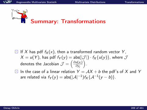
Angewandte Multivariate Statistik Multivariate Distributions Transformations
Summary: Transformations
If X has pdf fX (x), then a transformed random vector Y ,X = u(Y ), has pdf fY (y) = abs(|J |) · fXu(y), where Jdenotes the Jacobian J =
(∂u(yi )∂yj
).
In the case of a linear relation Y = AX + b the pdf’s of X and Yare related via fY (y) = abs(|A|−1)fXA−1(y − b).
Ostap Okhrin 209 of 461
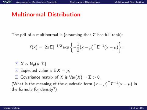
Angewandte Multivariate Statistik Multivariate Distributions Multinormal Distribution
Multinormal Distribution
The pdf of a multinormal is (assuming that Σ has full rank):
f (x) = |2πΣ|−1/2 exp−12
(x − µ)>Σ−1(x − µ)
.
X ∼ Np(µ,Σ)
Expected value is EX = µ,
Covariance matrix of X is Var(X ) = Σ > 0.(What is the meaning of the quadratic form (x − µ)>Σ−1(x − µ) inthe formula for density?)
Ostap Okhrin 210 of 461

Angewandte Multivariate Statistik Multivariate Distributions Multinormal Distribution
Geometry of the Np(µ,Σ) Distribution
Density of Np(µ,Σ) is constant on ellipsoids of the form
(x − µ)>Σ−1(x − µ) = d2
If X ∼ Np(µ,Σ), then the variable Y = (X − µ)>Σ−1(X − µ) is χ2p
distributed, since the Mahalanobis transformation yieldsZ = Σ−1/2(X − µ) ∼ Np(0, Ip) and Y = Z>Z =
∑pj=1 Z
2j .
Ostap Okhrin 211 of 461
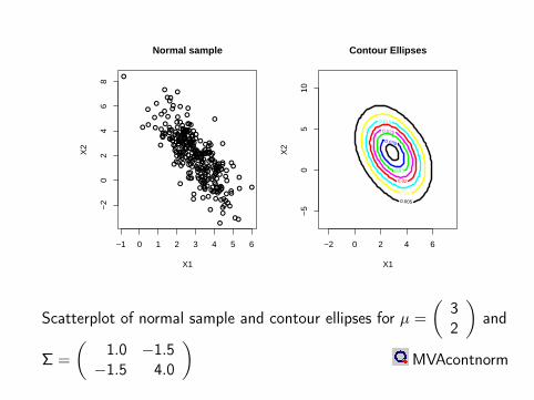
−1 0 1 2 3 4 5 6
−2
02
46
8
X1
X2
Normal sample
X1
X2
0.005
0.01
0.015
0.02
0.025
0.03
0.035
−2 0 2 4 6
−5
05
10
Contour Ellipses
Scatterplot of normal sample and contour ellipses for µ =
(32
)and
Σ =
(1.0 −1.5−1.5 4.0
)MVAcontnorm

Angewandte Multivariate Statistik Multivariate Distributions Multinormal Distribution
Singular Normal Distribution
Definition of “Normal” distribution in case that the matrix Σ issingular-we use its eigenvalues λi and the generalized inverse Σ−:rank(Σ) = k < p, λ1, . . . , λk
f (x) =(2π)−k/2
(λ1 · · ·λk)1/2 exp−12
(x − µ)>Σ−(x − µ)
Σ− = G-inverse
Ostap Okhrin 213 of 461
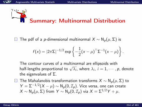
Angewandte Multivariate Statistik Multivariate Distributions Multinormal Distribution
Summary: Multinormal Distribution
The pdf of a p-dimensional multinormal X ∼ Np(µ,Σ) is
f (x) = |2πΣ|−1/2 exp−12
(x − µ)>Σ−1(x − µ)
.
The contour curves of a multinormal are ellipsoids withhalf-lengths proportional to
√λi , where λi , i = 1, · · · , p, denote
the eigenvalues of Σ. The Mahalanobis transformation transforms X ∼ Np(µ,Σ) to
Y = Σ−1/2(X − µ) ∼ Np(0, Ip). Vice versa, one can createX ∼ Np(µ,Σ) from Y ∼ Np(0, Ip) via X = Σ1/2Y + µ.
Ostap Okhrin 214 of 461
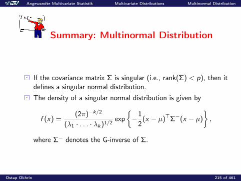
Angewandte Multivariate Statistik Multivariate Distributions Multinormal Distribution
Summary: Multinormal Distribution
If the covariance matrix Σ is singular (i.e., rank(Σ) < p), then itdefines a singular normal distribution.
The density of a singular normal distribution is given by
f (x) =(2π)−k/2
(λ1 · . . . · λk)1/2 exp−12
(x − µ)>Σ−(x − µ)
,
where Σ− denotes the G-inverse of Σ.
Ostap Okhrin 215 of 461
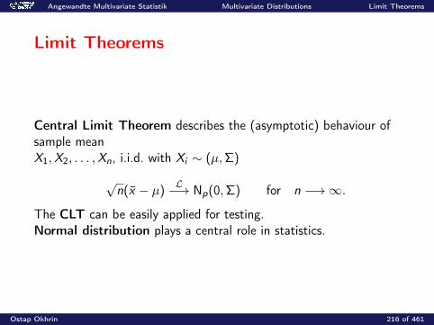
Angewandte Multivariate Statistik Multivariate Distributions Limit Theorems
Limit Theorems
Central Limit Theorem describes the (asymptotic) behaviour ofsample meanX1,X2, . . . ,Xn, i.i.d. with Xi ∼ (µ,Σ)
√n(x − µ)
L−→ Np(0,Σ) for n −→∞.
The CLT can be easily applied for testing.Normal distribution plays a central role in statistics.
Ostap Okhrin 216 of 461
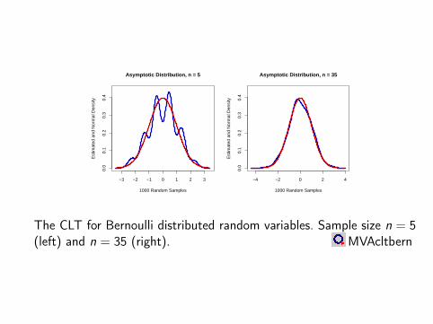
−3 −2 −1 0 1 2 3
0.0
0.1
0.2
0.3
0.4
1000 Random Samples
Est
imat
ed a
nd N
orm
al D
ensi
ty
Asymptotic Distribution, n = 5
−4 −2 0 2 4
0.0
0.1
0.2
0.3
0.4
1000 Random Samples
Est
imat
ed a
nd N
orm
al D
ensi
ty
Asymptotic Distribution, n = 35
The CLT for Bernoulli distributed random variables. Sample size n = 5(left) and n = 35 (right). MVAcltbern
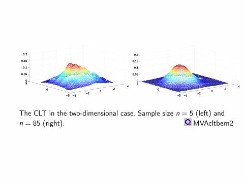
−4−2
02
4
−5
0
50
0.05
0.1
0.15
0.2
−4−2
02
4
−5
0
50
0.05
0.1
0.15
0.2
The CLT in the two-dimensional case. Sample size n = 5 (left) andn = 85 (right). MVAcltbern2
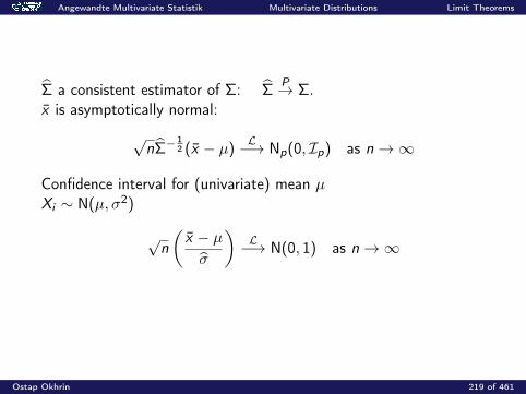
Angewandte Multivariate Statistik Multivariate Distributions Limit Theorems
Σ a consistent estimator of Σ: ΣP→ Σ.
x is asymptotically normal:
√nΣ−
12 (x − µ)
L−→ Np(0, Ip) as n→∞
Confidence interval for (univariate) mean µXi ∼ N(µ, σ2)
√n
(x − µσ
)L−→ N(0, 1) as n→∞
Ostap Okhrin 219 of 461

Angewandte Multivariate Statistik Multivariate Distributions Limit Theorems
Define u1−α/2 as the 1− α/2 quantile of the N(0, 1) distribution.Then we get the following 1− α confidence interval:
C1−α =
[x − σ√
nu1−α/2, x +
σ√nu1−α/2
]P(µ ∈ C1−α) −→ 1− α for n→∞.
Ostap Okhrin 220 of 461
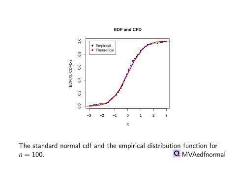
−3 −2 −1 0 1 2 3
0.0
0.2
0.4
0.6
0.8
1.0
EDF and CFD
X
ED
F(X
), C
DF
(X)
EmpiricalTheoretical
The standard normal cdf and the empirical distribution function forn = 100. MVAedfnormal
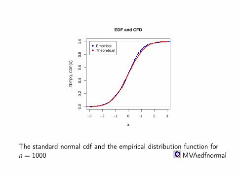
−3 −2 −1 0 1 2 3
0.0
0.2
0.4
0.6
0.8
1.0
EDF and CFD
X
ED
F(X
), C
DF
(X)
EmpiricalTheoretical
The standard normal cdf and the empirical distribution function forn = 1000 MVAedfnormal
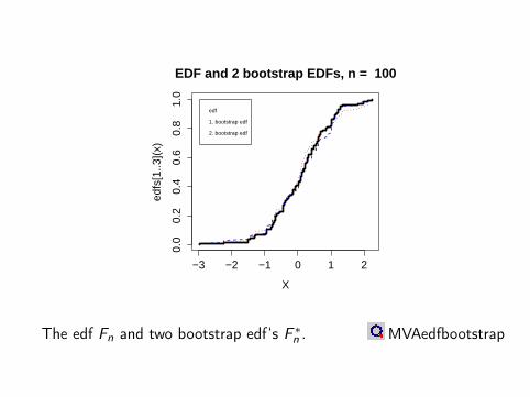
−3 −2 −1 0 1 2
0.0
0.2
0.4
0.6
0.8
1.0
X
edfs
[1..3
](x)
EDF and 2 bootstrap EDFs, n = 100
edf
1. bootstrap edf
2. bootstrap edf
The edf Fn and two bootstrap edf‘s F ∗n . MVAedfbootstrap
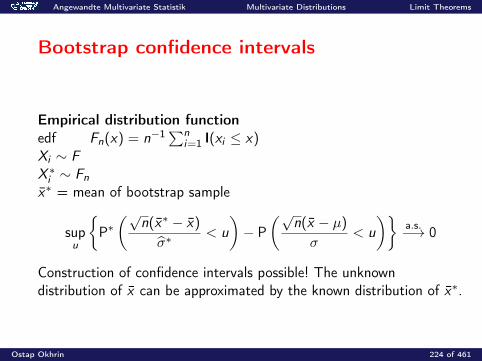
Angewandte Multivariate Statistik Multivariate Distributions Limit Theorems
Bootstrap confidence intervals
Empirical distribution functionedf Fn(x) = n−1∑n
i=1 I(xi ≤ x)Xi ∼ FX ∗i ∼ Fnx∗ = mean of bootstrap sample
supu
P∗(√
n(x∗ − x)
σ∗< u
)− P
(√n(x − µ)
σ< u
)a.s.−→ 0
Construction of confidence intervals possible! The unknowndistribution of x can be approximated by the known distribution of x∗.
Ostap Okhrin 224 of 461
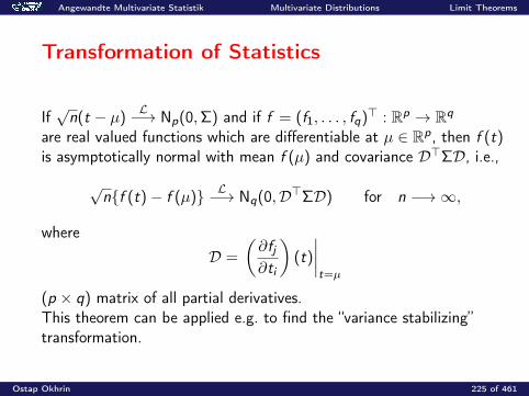
Angewandte Multivariate Statistik Multivariate Distributions Limit Theorems
Transformation of Statistics
If√n(t − µ)
L−→ Np(0,Σ) and if f = (f1, . . . , fq)> : Rp → Rq
are real valued functions which are differentiable at µ ∈ Rp, then f (t)is asymptotically normal with mean f (µ) and covariance D>ΣD, i.e.,
√nf (t)− f (µ) L−→ Nq(0,D>ΣD) for n −→∞,
where
D =
(∂fj∂ti
)(t)
∣∣∣∣t=µ
(p × q) matrix of all partial derivatives.This theorem can be applied e.g. to find the “variance stabilizing”transformation.
Ostap Okhrin 225 of 461
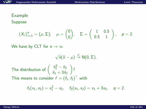
Angewandte Multivariate Statistik Multivariate Distributions Limit Theorems
ExampleSuppose
Xini=1 ∼ (µ,Σ); µ =
(00
), Σ =
(1 0.50.5 1
), p = 2.
We have by CLT for n→∞√n(x − µ)
L→ N(0,Σ).
The distribution of(
x21 − x2
x1 + 3x2
)?
This means to consider f = (f1, f2)> with
f1(x1, x2) = x21 − x2, f2(x1, x2) = x1 + 3x2, q = 2.
Ostap Okhrin 226 of 461

Angewandte Multivariate Statistik Multivariate Distributions Limit Theorems
Then f (µ) =(00
)and
D = (dij), dij =
(∂fj∂xi
)∣∣∣∣x=µ
=
(2x1 1−1 3
)∣∣∣∣x=0
=
(0 1−1 3
).
We have the covariance(0 −11 3
) (1 1
212 1
) (0 1−1 3
)=
(1 −7
2−7
2 13
)D> Σ D D>ΣD
.
This yields
√n
(x21 − x2
x1 + 3x2
)L→ N2
((00
),
(1 −7
2−7
2 13
)).
Ostap Okhrin 227 of 461
Angewandte Multivariate Statistik Multivariate Distributions Limit Theorems
Summary: Limit Theorems
If X1, . . . ,Xn are i.i.d. random vectors with Xi ∼ (µ,Σ), then thedistribution of
√n(x − µ) is asymptotically N(0,Σ) (Central Limit
Theorem). If X1, . . . ,Xn are i.i.d. random variables with Xi ∼ (µ, σ), then an
asymptotic confidence interval can be constructed by the CLT:
x ± σ√nu1−α/2.
Ostap Okhrin 228 of 461
Angewandte Multivariate Statistik Multivariate Distributions Limit Theorems
Summary: Limit Theorems
For small sample sizes the Bootstrap improves the precision ofthis confidence interval.
The Bootstrap estimates x∗ have the same asymptotic limit. If t is a statistic that is asymptotically normal, i.e.,√n(t − µ)
L→ Np(0,Σ), then this holds also for a function f (t),i.e.,√nf (t)− f (µ) is asymptotically normal.
Ostap Okhrin 229 of 461

Angewandte Multivariate Statistik Multivariate Distributions Heavy-Tailed Distributions
Heavy-Tailed Distributions
Introduced by Pareto, studied by Paul Lévy Applications: finance, medicine, seismology, engineering
I asset returns in financial marketsI stream flow in hydrologyI insuranceI precipitation and hurricane damage in meteorologyI earthquake prediction in seismologyI pollutionI material strength
Ostap Okhrin 230 of 461

Angewandte Multivariate Statistik Multivariate Distributions Heavy-Tailed Distributions
Definition
A distribution is called heavy-tailed if it has higher probability densityin its tail area compared with a normal distribution with same mean µand variance σ2.
Ostap Okhrin 231 of 461
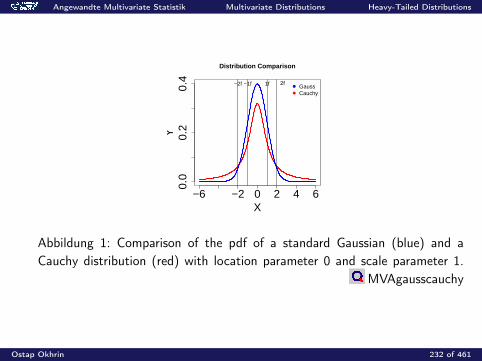
Angewandte Multivariate Statistik Multivariate Distributions Heavy-Tailed Distributions
−6 −2 0 2 4 60.
00.
20.
4
X
Y
−2f −1f 1f 2f
GaussCauchy
Distribution Comparison
Abbildung 1: Comparison of the pdf of a standard Gaussian (blue) and aCauchy distribution (red) with location parameter 0 and scale parameter 1.
MVAgausscauchy
Ostap Okhrin 232 of 461
Angewandte Multivariate Statistik Multivariate Distributions Heavy-Tailed Distributions
Kurtosis
In terms of kurtosis, a heavy-tailed distribution has kurtosis greaterthan 3, which is called leptokurtic, in contrast to mesokurticdistribution (kurtosis = 3) and platykurtic distribution (kurtosis < 3).
Ostap Okhrin 233 of 461

Angewandte Multivariate Statistik Multivariate Distributions Heavy-Tailed Distributions
Generalised Hyperbolic Distribution
Introduced by Barndorff-Nielsen and at first applied to model grainsize distributions of wind blown sands.Applications: stock price modelling, market risk measurement.
Ostap Okhrin 234 of 461
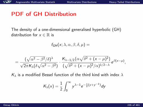
Angewandte Multivariate Statistik Multivariate Distributions Heavy-Tailed Distributions
PDF of GH Distribution
The density of a one-dimensional generalised hyperbolic (GH)distribution for x ∈ R is
fGH(x ;λ, α, β, δ, µ) =
=(√α2 − β2/δ)λ
√2πKλ(δ
√α2 − β2)
·Kλ−1/2α
√δ2 + (x − µ)2
(√δ2 + (x − µ)2/α)1/2−λ
eβ(x−µ),
Kλ is a modified Bessel function of the third kind with index λ
Kλ(x) =12
∫ ∞0
yλ−1e−x2 (y+y−1)dy
Ostap Okhrin 235 of 461
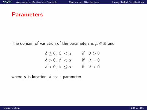
Angewandte Multivariate Statistik Multivariate Distributions Heavy-Tailed Distributions
Parameters
The domain of variation of the parameters is µ ∈ R and
δ ≥ 0, |β| < α, if λ > 0δ > 0, |β| < α, if λ = 0δ > 0, |β| ≤ α, if λ < 0
where µ is location, δ scale parameter.
Ostap Okhrin 236 of 461
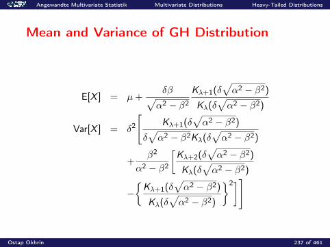
Angewandte Multivariate Statistik Multivariate Distributions Heavy-Tailed Distributions
Mean and Variance of GH Distribution
E[X ] = µ+δβ√α2 − β2
Kλ+1(δ√α2 − β2)
Kλ(δ√α2 − β2)
Var[X ] = δ2
[Kλ+1(δ
√α2 − β2)
δ√α2 − β2Kλ(δ
√α2 − β2)
+β2
α2 − β2
[Kλ+2(δ
√α2 − β2)
Kλ(δ√α2 − β2)
−Kλ+1(δ
√α2 − β2)
Kλ(δ√α2 − β2)
2]]
Ostap Okhrin 237 of 461
Angewandte Multivariate Statistik Multivariate Distributions Heavy-Tailed Distributions
Hyperbolic and Normal-Inverse GaussianDistributions
With specific values of λ we obtain different sub-classes of GH.
For λ = 1 we obtain the hyperbolic distributions (HYP)
fHYP(x ;α, β, δ, µ) =
√α2 − β2
2αδK1(δ√α2 − β2)
e−α√δ2+(x−µ)2+β(x−µ)
where x , µ ∈ R, δ ≥ 0 and |β| < α.
For λ = −1/2 we obtain the normal-inverse Gaussian distribution(NIG)
fNIG (x ;α, β, δ, µ) =αδ
π
K1(α√
(δ2 + (x − µ)2))√
δ2 + (x − µ)2eδ√α2−β2+β(x−µ).
Ostap Okhrin 238 of 461
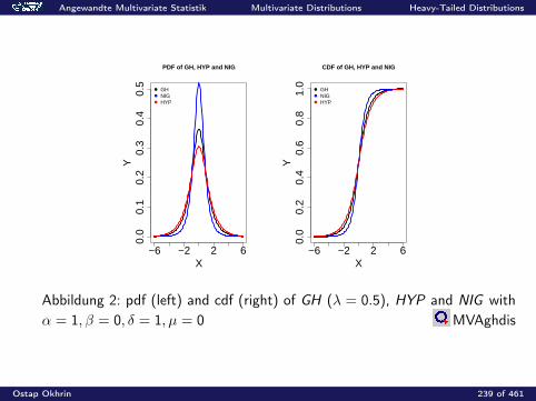
Angewandte Multivariate Statistik Multivariate Distributions Heavy-Tailed Distributions
−6 −2 2 6
0.0
0.1
0.2
0.3
0.4
0.5
X
Y
GHNIGHYP
PDF of GH, HYP and NIG
−6 −2 2 6
0.0
0.2
0.4
0.6
0.8
1.0
X
Y
GHNIGHYP
CDF of GH, HYP and NIG
Abbildung 2: pdf (left) and cdf (right) of GH (λ = 0.5), HYP and NIG withα = 1, β = 0, δ = 1, µ = 0 MVAghdis
Ostap Okhrin 239 of 461

Angewandte Multivariate Statistik Multivariate Distributions Heavy-Tailed Distributions
Student’s t-distribution
Introduced by Gosset (1908). Published under the pseudonymßtudent"by request of his employer.Let X be a normally distributed rv with mean µ and variance σ2, andY be the rv such that Y 2/σ2 has a chi-square distribution with ndegrees of freedom. Assume that X and Y are independent, then
tdef=
X√n
Y
is distributed as Student’s t with n degrees of freedom.
Ostap Okhrin 240 of 461

Angewandte Multivariate Statistik Multivariate Distributions Heavy-Tailed Distributions
PDF of Student’s t-distribution
The t-distribution has the following density function
ft(x ; n) =Γ(n+12
)√nπΓ
(n2
)(1 +x2
n
)− n+12
where n is the number of degrees of freedom, −∞ < x <∞, and Γ isthe gamma function
Γ(α) =
∫ ∞0
xα−1e−xdx
Ostap Okhrin 241 of 461
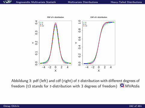
Angewandte Multivariate Statistik Multivariate Distributions Heavy-Tailed Distributions
−4 −2 0 2 4
0.0
0.1
0.2
0.3
0.4
X
Y
t3t6t30
PDF of t−distribution
−4 −2 0 2 4
0.0
0.2
0.4
0.6
0.8
1.0
X
Y
t3t6t30
CDF of t−distribution
Abbildung 3: pdf (left) and cdf (right) of t-distribution with different degrees offreedom (t3 stands for t-distribution with 3 degrees of freedom) MVAtdis
Ostap Okhrin 242 of 461
Angewandte Multivariate Statistik Multivariate Distributions Heavy-Tailed Distributions
Mean, Variance, Skewness and Kurtosis
The mean, variance, skewness and kurtosis of Student’s t-distribution(n > 4) are:
µ = 0
σ2 =n
n − 2Skewness = 0
Kurtosis = 3 +6
n − 4.
Ostap Okhrin 243 of 461

Angewandte Multivariate Statistik Multivariate Distributions Heavy-Tailed Distributions
Property
Student’s t-distribution approaches the normal distribution as nincreases, since
limn→∞
ft(x ; n) =1√2π
e−x22 .
Ostap Okhrin 244 of 461
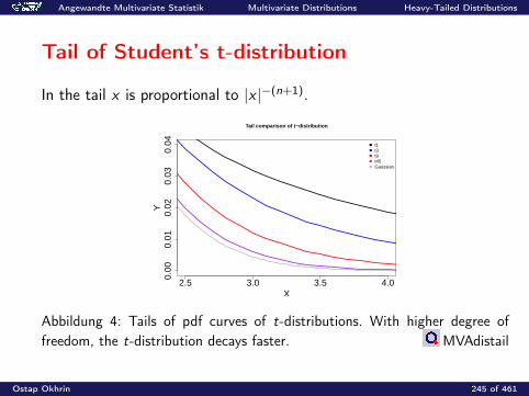
Angewandte Multivariate Statistik Multivariate Distributions Heavy-Tailed Distributions
Tail of Student’s t-distribution
In the tail x is proportional to |x |−(n+1).
2.5 3.0 3.5 4.0
0.00
0.01
0.02
0.03
0.04
X
Y
t1t3t9t45Gaussian
Tail comparison of t−distribution
Abbildung 4: Tails of pdf curves of t-distributions. With higher degree offreedom, the t-distribution decays faster. MVAdistail
Ostap Okhrin 245 of 461
Angewandte Multivariate Statistik Multivariate Distributions Heavy-Tailed Distributions
Laplace Distribution
The univariate Laplace distribution with mean zero was introduced byLaplace (1774).The Laplace distribution can be defined as the distribution ofdifferences between two independent variates with identicalexponential distributions.
Ostap Okhrin 246 of 461
Angewandte Multivariate Statistik Multivariate Distributions Heavy-Tailed Distributions
PDF and CDF of Laplace Distribution
The Laplace distribution with mean µ and scale parameter θ has thepdf
fLaplace(x ;µ, θ) =12θ
e−|x−µ|θ
and the cdf
FLaplace(x ;µ, θ) =121 + sgn(x − µ)(1− e−
|x−µ|θ ),
where sgn is signum function.
Ostap Okhrin 247 of 461
Angewandte Multivariate Statistik Multivariate Distributions Heavy-Tailed Distributions
Mean, Variance, Skewness and Kurtosis
The mean, variance, skewness and kurtosis of the Laplace distribution:
µ = µ
σ2 = 2θ2
Skewness = 0Kurtosis = 6
Ostap Okhrin 248 of 461
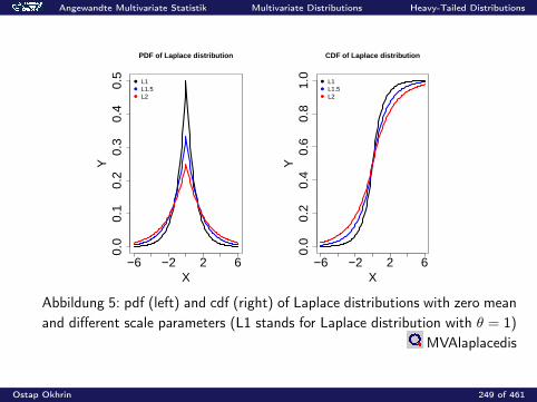
Angewandte Multivariate Statistik Multivariate Distributions Heavy-Tailed Distributions
−6 −2 2 6
0.0
0.1
0.2
0.3
0.4
0.5
X
Y
L1L1.5L2
PDF of Laplace distribution
−6 −2 2 6
0.0
0.2
0.4
0.6
0.8
1.0
XY
L1L1.5L2
CDF of Laplace distribution
Abbildung 5: pdf (left) and cdf (right) of Laplace distributions with zero meanand different scale parameters (L1 stands for Laplace distribution with θ = 1)
MVAlaplacedis
Ostap Okhrin 249 of 461
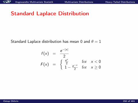
Angewandte Multivariate Statistik Multivariate Distributions Heavy-Tailed Distributions
Standard Laplace Distribution
Standard Laplace distribution has mean 0 and θ = 1
f (x) =e−|x |
2
F (x) =
ex
2 for x < 01− e−x
2 for x ≥ 0
Ostap Okhrin 250 of 461

Angewandte Multivariate Statistik Multivariate Distributions Heavy-Tailed Distributions
Cauchy Distribution
Named after Augustin Cauchy and Hendrik Lorentz.Applications in physics – the solution to the differential equation describing
forced resonance, in spectroscopy – the description of the line shape of spectral
lines.
Ostap Okhrin 251 of 461

Angewandte Multivariate Statistik Multivariate Distributions Heavy-Tailed Distributions
PDF and CDF of the Cauchy Distribution
fCauchy (x ;m, s) =1sπ
11 + ( x−ms )2
FCauchy (x ;m, s) =12
+1πarctan
(x −m
s
)where m and s are location and scale parameter respectively.
Ostap Okhrin 252 of 461
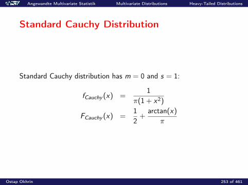
Angewandte Multivariate Statistik Multivariate Distributions Heavy-Tailed Distributions
Standard Cauchy Distribution
Standard Cauchy distribution has m = 0 and s = 1:
fCauchy (x) =1
π(1 + x2)
FCauchy (x) =12
+arctan(x)
π
Ostap Okhrin 253 of 461
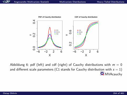
Angewandte Multivariate Statistik Multivariate Distributions Heavy-Tailed Distributions
−6 −2 2 6
0.0
0.2
0.4
X
Y
C1C1.5C2
PDF of Cauchy distribution
−6 −2 2 6
0.2
0.6
X
Y
C1C1.5C2
CDF of Cauchy distribution
Abbildung 6: pdf (left) and cdf (right) of Cauchy distributions with m = 0and different scale parameters (C1 stands for Cauchy distribution with s = 1)
MVAcauchy
Ostap Okhrin 254 of 461
Angewandte Multivariate Statistik Multivariate Distributions Heavy-Tailed Distributions
Mean, Variance, Skewness and Kurtosis
The mean, variance, skewness and kurtosis of Cauchy distribution areall undefined, since its moment generating function diverges. But ithas mode and median, both equal the location parameter m.
Ostap Okhrin 255 of 461

Angewandte Multivariate Statistik Multivariate Distributions Heavy-Tailed Distributions
Mixture Model
Mixture modelling concerns modelling a distribution by a mixture(weighted sum) of different distributions.
Ostap Okhrin 256 of 461

Angewandte Multivariate Statistik Multivariate Distributions Heavy-Tailed Distributions
PDF of Mixture Model
The pdf of a mixture distribution
f (x) =n∑
l=1
wlpl(x)
under the constraints:
0 ≤ wl ≤ 1n∑
l=1
wl = 1∫pl(x)dx = 1,
pl(x) is the pdf of the l ’th component density and wl is a weight.
Ostap Okhrin 257 of 461
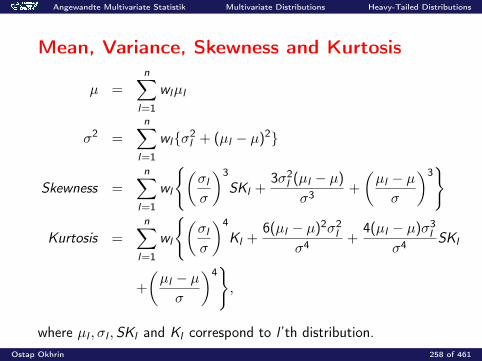
Angewandte Multivariate Statistik Multivariate Distributions Heavy-Tailed Distributions
Mean, Variance, Skewness and Kurtosis
µ =n∑
l=1
wlµl
σ2 =n∑
l=1
wlσ2l + (µl − µ)2
Skewness =n∑
l=1
wl
(σlσ
)3
SKl +3σ2
l (µl − µ)
σ3 +
(µl − µσ
)3
Kurtosis =n∑
l=1
wl
(σlσ
)4
Kl +6(µl − µ)2σ2
l
σ4 +4(µl − µ)σ3
l
σ4 SKl
+
(µl − µσ
)4,
where µl , σl ,SKl and Kl correspond to l ’th distribution.Ostap Okhrin 258 of 461
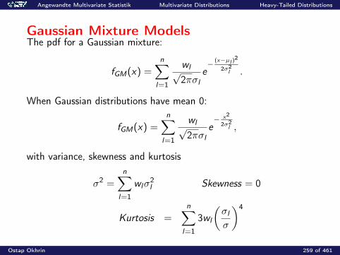
Angewandte Multivariate Statistik Multivariate Distributions Heavy-Tailed Distributions
Gaussian Mixture ModelsThe pdf for a Gaussian mixture:
fGM(x) =n∑
l=1
wl√2πσl
e− (x−µl )
2
2σ2l .
When Gaussian distributions have mean 0:
fGM(x) =n∑
l=1
wl√2πσl
e− x2
2σ2l ,
with variance, skewness and kurtosis
σ2 =n∑
l=1
wlσ2l Skewness = 0
Kurtosis =n∑
l=1
3wl
(σlσ
)4
Ostap Okhrin 259 of 461
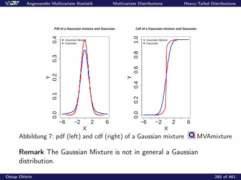
Angewandte Multivariate Statistik Multivariate Distributions Heavy-Tailed Distributions
−6 −2 2 6
0.0
0.1
0.2
0.3
0.4
X
Y
Gaussian MixtureGaussian
Pdf of a Gaussian mixture and Gaussian
−6 −2 2 6
0.0
0.2
0.4
0.6
0.8
1.0
XY
Gaussian MixtureGaussian
Cdf of a Gaussian mixture and Gaussian
Abbildung 7: pdf (left) and cdf (right) of a Gaussian mixture MVAmixture
Remark The Gaussian Mixture is not in general a Gaussiandistribution.
Ostap Okhrin 260 of 461

Angewandte Multivariate Statistik Multivariate Distributions Heavy-Tailed Distributions
Multivariate Generalised HyperbolicDistribution
The multivariate Generalised Hyperbolic Distribution (GHd) has thefollowing pdf
fGHd (x ;λ, α, β, δ,∆, µ) = adKλ− d
2
α√δ2 + (x − µ)>∆−1(x − µ)
α−1
√δ2 + (x − µ)>∆−1(x − µ)
d2−λ
eβ>(x−µ)
ad = ad(λ, α, β, δ,∆) =
(√α2 − β>∆β/δ
)λ(2π)
d2 Kλ(δ
√α2 − β>∆β
.
Ostap Okhrin 261 of 461
Angewandte Multivariate Statistik Multivariate Distributions Heavy-Tailed Distributions
Parameters of GHd
The domain of variation of the parameters:
λ ∈ R, β, µ ∈ Rd
δ > 0, α > β>∆β∆ ∈ Rd×d positive definite matrix|∆| = 1
For λ = d+12 we obtain the multivariate hyperbolic (HYP) distribution;
for λ = −12 we get the multivariate normal inverse Gaussian (NIG)
distribution.
Ostap Okhrin 262 of 461
Angewandte Multivariate Statistik Multivariate Distributions Heavy-Tailed Distributions
Second Parameterization
Blæsild and Jensen (1981) introduced a second parameterization(ζ,Π,Σ), where
ζ = δ√α2 − β>∆β
Π = β
√∆
α2 − β>∆β
Σ = δ2∆
Ostap Okhrin 263 of 461
Angewandte Multivariate Statistik Multivariate Distributions Heavy-Tailed Distributions
Second Parameterization
The mean and variance of X ∼ GHd
E[X ] = µ+ δRλ(ζ)Π∆12
Var[X ] = δ2ζ−1Rλ(ζ)∆ + Sλ(ζ)(Π∆
12 )>(Π∆
12 )
where
Rλ(x) =Kλ+1(x)
Kλ(x)
Sλ(x) =Kλ+2(x)Kλ(x)− K 2
λ+1(x)
K 2λ(x)
Ostap Okhrin 264 of 461
Angewandte Multivariate Statistik Multivariate Distributions Heavy-Tailed Distributions
Multivariate t-distribution
If X ∼ Np(µ,Σ) and Y ∼ χ2n are independent and X
√n/Y = t − µ,
then the pdf of t is
ft(t; n,Σ, µ) =Γ (n + p)/2
Γ(n/2)np/2πp/2 |Σ|1/21 + 1
n (t − µ)>Σ−1(t − µ)(n+p)/2
The distribution of t is the noncentral t-distribution with n degrees offreedom and the noncentrality parameter µ.
Ostap Okhrin 265 of 461
Angewandte Multivariate Statistik Multivariate Distributions Heavy-Tailed Distributions
Multivariate Laplace Distribution
Let g and G be the pdf and cdf of a d-dimensional Gaussiandistribution Nd(0,Σ), the pdf and cdf of a multivariate Laplacedistribution can be written as
fMLaplaced (x ;m,Σ) =
∫ ∞0
g(z−12 x − z
12m)z−
d2 e−zdz
FMLaplaced (x ,m,Σ) =
∫ ∞0
G (z−12 x − z
12m)e−zdz
Ostap Okhrin 266 of 461
Angewandte Multivariate Statistik Multivariate Distributions Heavy-Tailed Distributions
PDF of Multivariate Laplace Distribution
The pdf can also be described as
fMLaplaced (x ;m,Σ) =2ex
>Σ−1m
(2π)d2 |Σ|
12
(x>Σ−1x
2 + m>Σ−1m
)λ2
×Kλ(√
(2 + m>Σ−1m)(x>Σ−1x))
where λ = 2−d2 and Kλ(x) is the modified Bessel function of the third
kind
Kλ(x) =12
(x
2
)λ ∫ ∞0
t−λ−1e−t−x24t dt, x > 0
Ostap Okhrin 267 of 461
Angewandte Multivariate Statistik Multivariate Distributions Heavy-Tailed Distributions
Mean and Variance of Multivariate LaplaceDistribution
E[X ] = m
Cov[X ] = Σ + mm>
Ostap Okhrin 268 of 461
Angewandte Multivariate Statistik Multivariate Distributions Heavy-Tailed Distributions
Multivariate Mixture Model
A multivariate mixture model comprises multivariate distributions, e.g.the pdf of a multivariate Gaussian distribution can be written as
f (x) =n∑
l=1
wl
|2πΣl |12e−
12 (x−µl )>Σ−1(x−µl )
Ostap Okhrin 269 of 461
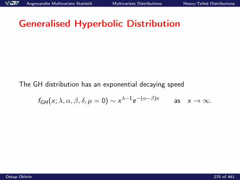
Angewandte Multivariate Statistik Multivariate Distributions Heavy-Tailed Distributions
Generalised Hyperbolic Distribution
The GH distribution has an exponential decaying speed
fGH(x ;λ, α, β, δ, µ = 0) ∼ xλ−1e−(α−β)x as x →∞.
Ostap Okhrin 270 of 461
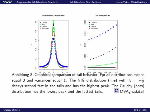
Angewandte Multivariate Statistik Multivariate Distributions Heavy-Tailed Distributions
−6 −4 −2 0 2 4 6
0.0
0.1
0.2
0.3
0.4
0.5
X
Y
LaplaceNIGCauchyGaussian
Distribution comparison
−5.0 −4.8 −4.6 −4.4 −4.2 −4.0
0.00
00.
005
0.01
00.
015
0.02
0
X
Y
LaplaceNIGCauchyGaussian
Tail comparison
Abbildung 8: Graphical comparison of tail behavior. For all distributions meansequal 0 and variances equal 1. The NIG distribution (line) with λ = − 1
2decays second fast in the tails and has the highest peak. The Cauchy (dots)distribution has the lowest peak and the fattest tails. MVAghadatail
Ostap Okhrin 271 of 461

Angewandte Multivariate Statistik Multivariate Distributions Copulae
Copulae vs Normal Distribution
1. The empirical marginal distributions are skewed and fat tailed.2. Multivariate normal distribution does not consider the possibility
of extreme joint co-movement of asset returns.The dependency structure of portfolio asset returns is differentfrom the Gaussian one.
Ostap Okhrin 272 of 461
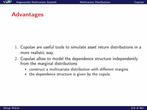
Angewandte Multivariate Statistik Multivariate Distributions Copulae
Advantages
1. Copulae are useful tools to simulate asset return distributions in amore realistic way.
2. Copulae allow to model the dependence structure independentlyfrom the marginal distributions
I construct a multivariate distribution with different marginsI the dependence structure is given by the copula.
Ostap Okhrin 273 of 461
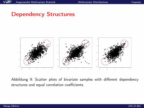
Angewandte Multivariate Statistik Multivariate Distributions Copulae
Dependency Structures
−4 −2 0 2 4
−4
−2
02
4
−4 −2 0 2 4
−4
−2
02
4
−4 −2 0 2 4
−4
−2
02
4
Abbildung 9: Scatter plots of bivariate samples with different dependencystructures and equal correlation coefficients.
Ostap Okhrin 274 of 461
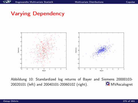
Angewandte Multivariate Statistik Multivariate Distributions Copulae
Varying Dependency
−4 −3 −2 −1 0 1 2 3 4−4
−3
−2
−1
0
1
2
3
4
Bayer
Sie
men
s
−4 −3 −2 −1 0 1 2 3 4−4
−3
−2
−1
0
1
2
3
4
Bayer
Sie
men
s
Abbildung 10: Standardized log returns of Bayer and Siemens 20000103-20020101 (left) and 20040101-20060102 (right). MVAscalogret
Ostap Okhrin 275 of 461

Angewandte Multivariate Statistik Multivariate Distributions Copulae
Outline
1. Motivation X2. Copulae3. Parameter Estimation4. Sampling from Copulae5. Tail Dependence6. Value-at-Risk with Copulae7. Application
Ostap Okhrin 276 of 461

Angewandte Multivariate Statistik Multivariate Distributions Copulae
Copulae
A copula is a multivariate distribution function defined on the unitcube [0, 1]d , with uniformly distributed margins.
P(X1 ≤ x1, . . . ,Xd ≤ xd) = C P(X1 ≤ x1), . . . ,P(Xd ≤ xd)= C F1(x1), . . . ,Fd(xd)
Ostap Okhrin 277 of 461

Angewandte Multivariate Statistik Multivariate Distributions Copulae
Applications
1. medicine2. hydrology3. finance (portfolio selection, time series, risk management)
2
the others work in banks, insurance companies and financial institutions. Their writings appeared in some 165 journals and conference proceedings. The most striking feature of the data set is the rapid growth in the annual number of contributions to the subject. This is illustrated in Figure 1. More detailed examination reveals that the growth falls into three periods:
a) Before 1986, the literature was sparse and mostly mathematical. The concept of copula can be traced back at least to the work of Wassily Hoeffding and Maurice Fréchet, though the term itself was coined by Sklar (1959). Many contributions were related to the study of probabilistic metric spaces, as described in the book by Schweizer & Sklar (1983).
b) Beginning in 1986, one can see a slow, systematic rise in the number of publications. Growth was largely due to the emergence of the concept of copula in statistics and to three conferences devoted to the subject: Rome (1990), Seattle (1993), and Prague (1996).
c) From 1999 on, the number of contributions grew considerably. The books by Joe (1997) and Nelsen (1999) were influential in disseminating copula theory; the book by Drouet-Mari & Kotz (2001), which focuses on correlation and dependence, is also noteworthy. Actuarial and financial applications were fuelled by Frees & Valdez (1998) and Embrechts et al. (1999), who illustrated the potential for copula modeling in these fields.
Figure 1. Number of documents on copula theory, 1971–2005 3. Breakdown by field of study What is the part of finance to the spectacular growth of copula methodology in the past few years? To investigate this issue, we subjectively grouped the 871 documents in our database into 9 mutually exclusive categories: mathematics; statistics; biostatistics; operations research; natural sciences; engineering; actuarial science; economics; and finance. We achieved this classification by carefully examining the contents of each document. About 1% of them did not match any of the categories and were left unclassified. Figure 2 shows the results of the grouping. Even though people in finance have been interested in copulas only since 2000, they produced the largest proportion of documents, i.e., 41%. Next come statistics (28%), biostatistics (10%), mathematics (8%), and actuarial science (8%). Interestingly, in June 2006 finance and actuarial science together contributed 47% of the literature, whereas mathematics, statistics, and biostatistics together accounted for 46%. No doubt
0 25 50 75
100 125 150 175 200 225
1972 1974 197619781980198219841986198819901992199419961998200020022004
3
finance-related documents now account for over half of the literature on the subject. We will later discuss the nature of these contributions.
2%
8%
10%
28%
41%
2%1% 1%
1%
6%
Unclassified Economics Operations research Engineering
Natural sciences Actuarial science Mathematics Biostatistics
Statistics Finance
Figure 2. Breakdown by discipline of the 871 documents in the database
The level of activity in each discipline is also reflected by Table 1, which lists the peer-review journals that carried the largest number of articles concerned with copulas. As of June 2006, statistics continued to lead the rooster. This is not surprising, given that copulas have a long history in this area. Interestingly, Risk Magazine and Quantitative Finance make the list, even though the earliest papers on the topic appeared there in 2001. A fair proportion of copula-related articles in Insurance: Mathematics and Economics also pertain to finance.
Table 1. List of journals that published the largest number of copula-related articles
Rank Journal Papers published
1 Journal of Multivariate Analysis 29 2 Statistics & Probability Letters 26 3 Insurance, Mathematics & Economics 23 4 Communications in Statistics: Theory & Methods 19 5 Biometrika 14 6 Risk 14 7 The Canadian Journal of Statistics 12 8 Biometrics 12 9 Quantitative Finance 11
10 Journal of Nonparametric Statistics 10
Abbildung 11: Number of documents on copula theory, 1971 - 2005. Break-down by discipline of the 871 documents in the database (41% Finance, 28%Statistics, 10% Biostatistics, 8% Mathematics, 6% Insurance)
Ostap Okhrin 278 of 461

Angewandte Multivariate Statistik Multivariate Distributions Copulae
F-volume
Let U1 and U2 be two sets in R = R ∪ +∞ ∪ −∞ and considerthe function F : U1 × U2 −→ R.The F -volume of a rectangle B = [x1, x2]× [y1, y2] ⊂ U1 × U2 isdefined as:
VF (B) = F (x2, y2)− F (x1, y2)− F (x2, y1) + F (x1, y1) (2)
Ostap Okhrin 279 of 461
Angewandte Multivariate Statistik Multivariate Distributions Copulae
2-increasing Function
F is said to be a 2-increasing function if for everyB = [x1, x2]× [y1, y2] ⊂ U1 × U2,
VF (B) ≥ 0 (3)
Remark Note, that “to be 2-increasing function” neither implies nor isimplied by “to be increasing in each argument”.
Ostap Okhrin 280 of 461
Angewandte Multivariate Statistik Multivariate Distributions Copulae
2-increasing Function
LemmaLet U1 and U2 be non-empty sets in R and let F : U1 ×U2 −→ R be atwo-increasing function. Let x1, x2 be in U1 with x1 ≤ x2, and y1, y2be in U2 with y1 ≤ y2. Then the function t 7→ F (t, y2)− F (t, y1) isnon-decreasing on U1 and the function t 7→ F (x2, t)− F (x1, t) isnon-decreasing on U2.
Ostap Okhrin 281 of 461
Angewandte Multivariate Statistik Multivariate Distributions Copulae
Grounded Function
If U1 and U2 have a smallest element minU1 and minU2 respectively,then we say, that a function F : U1 × U2 −→ R is grounded if :
for all x ∈ U1 : F (x ,minU2) = 0 and (4)for all y ∈ U2 : F (minU1, y) = 0 (5)
Ostap Okhrin 282 of 461
Angewandte Multivariate Statistik Multivariate Distributions Copulae
Distribution Function
A distribution function is a function from R2 7→ [0, 1] which: is grounded is 2-increasing satisfies F (∞,∞) = 1.
Ostap Okhrin 283 of 461

Angewandte Multivariate Statistik Multivariate Distributions Copulae
Margins
If U1 and U2 have a greatest element maxU1 and maxU2 respectively,then we say, that a function F : U1 × U2 −→ R has margins and thatthe margins of F are given by:
F (x) = F (x ,maxU2) for all x ∈ U1 (6)F (y) = F (maxU1, y) for all y ∈ U2 (7)
Ostap Okhrin 284 of 461
Angewandte Multivariate Statistik Multivariate Distributions Copulae
Bivariate Copulae
A 2-dimensional copula is a function C : [0, 1]2 → [0, 1] with thefollowing properties:1. For every u ∈ [0, 1], C (0, u) = C (u, 0) = 0 (grounded).2. For every u ∈ [0, 1], C (u, 1) = u and C (1, u) = u.
3. For every (u1, u2), (v1, v2) ∈ [0, 1]× [0, 1] with u1 ≤ v1 andu2 ≤ v2: C (v1, v2)− C (v1, u2)− C (u1, v2) + C (u1, u2) ≥ 0(2-increasing).
Ostap Okhrin 285 of 461
Angewandte Multivariate Statistik Multivariate Distributions Copulae
Fréchet-Hoeffding Bounds
1. every copula C satisfies
W (u1, u2) ≤ C (u1, u2) ≤ M(u1, u2)
2. upper and lower bounds are copulae
M(u1, u2) = min(u1, u2)
W (u1, u2) = max(u1 + u2 − 1, 0)
Ostap Okhrin 286 of 461
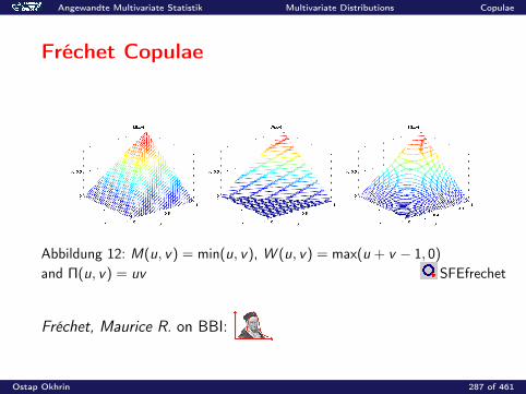
Angewandte Multivariate Statistik Multivariate Distributions Copulae
Fréchet Copulae
Abbildung 12: M(u, v) = min(u, v), W (u, v) = max(u + v − 1, 0)
and Π(u, v) = uv SFEfrechet
Fréchet, Maurice R. on BBI:
Ostap Okhrin 287 of 461
Angewandte Multivariate Statistik Multivariate Distributions Copulae
Sklar’s Theorem in Two Dimensions
Let F be a two-dimensional distribution function with marginaldistribution functions FX1 and FX2 . Then a copula C exists such thatfor all x1, x2 ∈ R2:
F (x1, x2) = CCC FX1 (x1) ,FX2 (x2) (8)
Moreover, if FX1 and FX2 are continuous, then C is unique. OtherwiseC is uniquely determined on the Cartesian product Im(FX1)× Im(FX2).Conversely, if C is a copula and FX1 and FX2 are distribution functions,then F defined by (24) is a two-dimensional distribution function withmarginals FX1 and FX2 .
Ostap Okhrin 288 of 461
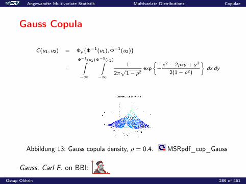
Angewandte Multivariate Statistik Multivariate Distributions Copulae
Gauss Copula
C(u1, u2) = ΦρΦ−1(u1),Φ−1(u2)
=
Φ−1(u1)∫−∞
Φ−1(u2)∫−∞
1
2π√
1− ρ2exp
−x2 − 2ρxy + y2
2(1− ρ2)
dx dy
Abbildung 13: Gauss copula density, ρ = 0.4. MSRpdf_cop_Gauss
Gauss, Carl F. on BBI:
Ostap Okhrin 289 of 461
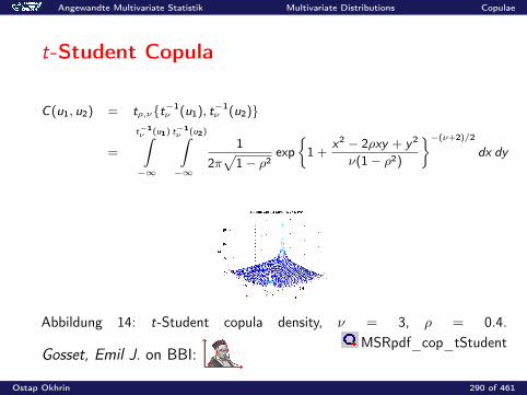
Angewandte Multivariate Statistik Multivariate Distributions Copulae
t-Student Copula
C(u1, u2) = tρ,νt−1ν (u1), t−1ν (u2)
=
t−1ν (u1)∫−∞
t−1ν (u2)∫−∞
12π√
1− ρ2exp
1 +
x2 − 2ρxy + y2
ν(1− ρ2)
−(ν+2)/2
dx dy
Abbildung 14: t-Student copula density, ν = 3, ρ = 0.4.MSRpdf_cop_tStudent
Gosset, Emil J. on BBI:
Ostap Okhrin 290 of 461

Angewandte Multivariate Statistik Multivariate Distributions Copulae
Archimedean Copulae
Archimedean copula:
C (u, v) = ψ[−1]ψ(u) + ψ(v)
for a continuous, decreasing and convex ψ, ψ(1) = 0.
ψ[−1](t) =
ψ−1(t), 0 ≤ t ≤ ψ(0),0, ψ(0) < t ≤ ∞.
The function ψ is a generator of the Archimedean copula.For ψ(0) =∞: ψ[−1] = ψ−1 and the ψ is called a strict generator.
Ostap Okhrin 291 of 461
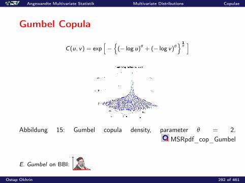
Angewandte Multivariate Statistik Multivariate Distributions Copulae
Gumbel Copula
C(u, v) = exp[−
(− log u)θ + (− log v)θ 1
θ]
Abbildung 15: Gumbel copula density, parameter θ = 2.MSRpdf_cop_Gumbel
E. Gumbel on BBI:
Ostap Okhrin 292 of 461
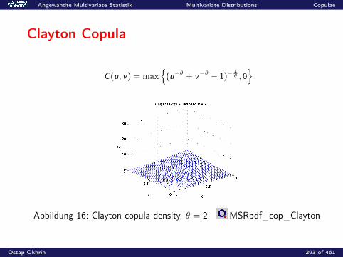
Angewandte Multivariate Statistik Multivariate Distributions Copulae
Clayton Copula
C(u, v) = max
(u−θ + v−θ − 1)−1θ , 0
Abbildung 16: Clayton copula density, θ = 2. MSRpdf_cop_Clayton
Ostap Okhrin 293 of 461
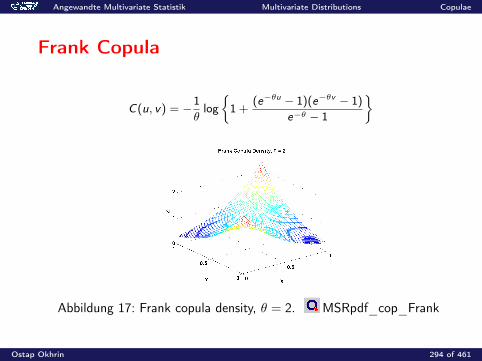
Angewandte Multivariate Statistik Multivariate Distributions Copulae
Frank Copula
C(u, v) = −1θ
log
1 +(e−θu − 1)(e−θv − 1)
e−θ − 1
Abbildung 17: Frank copula density, θ = 2. MSRpdf_cop_Frank
Ostap Okhrin 294 of 461
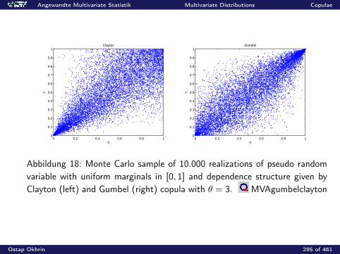
Angewandte Multivariate Statistik Multivariate Distributions Copulae
0 0.2 0.4 0.6 0.8 10
0.1
0.2
0.3
0.4
0.5
0.6
0.7
0.8
0.9
1
X
YClayton
0 0.2 0.4 0.6 0.8 10
0.1
0.2
0.3
0.4
0.5
0.6
0.7
0.8
0.9
1
X
Y
Gumbel
Abbildung 18: Monte Carlo sample of 10.000 realizations of pseudo randomvariable with uniform marginals in [0, 1] and dependence structure given byClayton (left) and Gumbel (right) copula with θ = 3. MVAgumbelclayton
Ostap Okhrin 295 of 461
Angewandte Multivariate Statistik Multivariate Distributions Copulae
Transformations of Margins
If (X1,X2) have copula C and set g1, g2 two continuous increasingfunctions, then g1 (X1) , g2 (X2) have the copula C, too.
Ostap Okhrin 296 of 461

Angewandte Multivariate Statistik Multivariate Distributions Copulae
Product Copula
Independence implies that the product of the cdf’s FX1 and FX2 equalsthe joint distribution function F , i.e.:
F (x1, x2) = FX1(x1)FX2(x2) (9)
Thus, we obtain the independence or product copulaC = Π(u, v) = uv .
Ostap Okhrin 297 of 461
Angewandte Multivariate Statistik Multivariate Distributions Copulae
Product Copula
Let X1 and X2 be random variables with continuous distributionfunctions F1 and F2 and joint distribution function H.Then X1 and X2 are independent if and only if CX1X2 = Π.According to Sklar’s Theorem, there exists a unique copula C with
P(X1 ≤ x1,X2 ≤ x2) = H(x1, x2)
= C F1(x1),F2(x2)= F1(x1) · F2(x2)
Ostap Okhrin 298 of 461

Angewandte Multivariate Statistik Multivariate Distributions Copulae
Partial DerivativesLet C (u, v) be a copula. For any v ∈ I , the partial derivative ∂C(u,v)
∂vexists for almost all u ∈ I . For such u and v one has:
∂C (u, v)
∂v∈ I (10)
The analogous statement is true for the partial derivative ∂C(u,v)∂u :
∂C (u, v)
∂u∈ I (11)
Moreover, the functions
u 7→ Cv (u)def= ∂C (u, v)/∂v and
v 7→ Cu(v)def= ∂C (u, v)/∂u
are defined and non-increasing almost everywhere on I .Ostap Okhrin 299 of 461

Angewandte Multivariate Statistik Multivariate Distributions Copulae
Copulae in d-Dimensions
Let U1,U2, . . . ,Ud be non-empty sets in R and consider the functionF : U1 × U2 × . . .× Ud −→ R. For a = (a1, a2, . . . , ad) andb = (b1, b2, . . . , bd) with a ≤ b (i.e. ak ≤ bk for all k) letB = [a, b] = [a1, b1]× [a2, b2]× . . .× [ad , bd ] be the d-box withvertices c = (c1, c2, . . . , cd). It is obvious, that each ck is either equalto ak or to bk .
Ostap Okhrin 300 of 461

Angewandte Multivariate Statistik Multivariate Distributions Copulae
F -volume
The F -volume of a d-boxB = [a, b] = [a1, b1]× [a2, b2]× . . .× [ad , bd ] ⊂ U1 ×U2 × . . .×Ud isdefined as follows:
VF (B) =d∑
k=1
sgn(ck)F (ck) (12)
where sgn(ck) = 1, if ck = ak for even k and sgn(ck) = −1, if ck = akfor odd k .
Ostap Okhrin 301 of 461
Angewandte Multivariate Statistik Multivariate Distributions Copulae
d-increasing Function
F is said to be a d-increasing function if for all d-boxes B with verticesin U1 × U2 × . . .× Ud holds:
VF (B) ≥ 0. (13)
Ostap Okhrin 302 of 461

Angewandte Multivariate Statistik Multivariate Distributions Copulae
Grounded Function
If U1,U2, . . . ,Ud have a smallest elementminU1,minU2, . . . ,minUd respectively, then we say, that a functionF : U1 × U2 × . . .× Ud −→ R is grounded if :
F (x) = 0 for all x ∈ U1 × U2 × . . .× Ud (14)
such that xk = minUk for at least one k.
Ostap Okhrin 303 of 461
Angewandte Multivariate Statistik Multivariate Distributions Copulae
Multivariate Copula
A d-dimensional copula is a function C : [0, 1]d → [0, 1]:1. C (u1, . . . , ui−1, 0, ui+1, . . . , ud) = 0 (at least one ui is 0);2. u ∈ [0, 1]d , C (1, . . . , 1, ui , 1, . . . , 1) = ui (all coordinates except
ui is 1)3. For each u < v ∈ [0, 1]d (ui < vi )
VC [u, v ] =∑a
sgn(a)C (a) ≥ 0
where a is taken over all vertices of [u, v ]. sgn(a) = 1 if ak = ukfor an even number of k ′s and sgn(a) = −1 if ak = uk for an oddnumber of k ′s (d-increasing).
Ostap Okhrin 304 of 461
Angewandte Multivariate Statistik Multivariate Distributions Copulae
Sklar’s Theorem
For a distribution function F with marginals FX1 . . . ,FXd, there exists
a copula C : [0, 1]d → [0, 1], such that
F (x1, . . . , xd) = CCCFX1(x1), . . . ,FXd(xd) (15)
for all xi ∈ R, i = 1, . . . , d . If FX1 , . . . ,FXdare cts, then C is unique.
If C is a copula and FX1 , . . . ,FXdare cdfs, then the function F defined
in (15) is a joint cdf with marginals FX1 , . . . ,FXd.
Ostap Okhrin 305 of 461
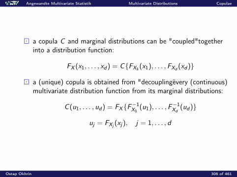
Angewandte Multivariate Statistik Multivariate Distributions Copulae
a copula C and marginal distributions can be "coupled"togetherinto a distribution function:
FX (x1, . . . , xd) = CFX1(x1), . . . ,FXd(xd)
a (unique) copula is obtained from "decouplingëvery (continuous)multivariate distribution function from its marginal distributions:
C (u1, . . . , ud) = FXF−1X1
(u1), . . . ,F−1Xd
(ud)
uj = FXj(xj), j = 1, . . . , d
Ostap Okhrin 306 of 461

Angewandte Multivariate Statistik Multivariate Distributions Copulae
if C is absolute continuous, there exists a copula density
c(u1, . . . , ud) =∂dC (u1, . . . , ud)
∂u1 . . .∂ud
the joint density fX is
fX (x1, . . . , xd) = cFX1(x1), . . . ,FXd(xd)
d∏j=1
fj(xj)
Ostap Okhrin 307 of 461
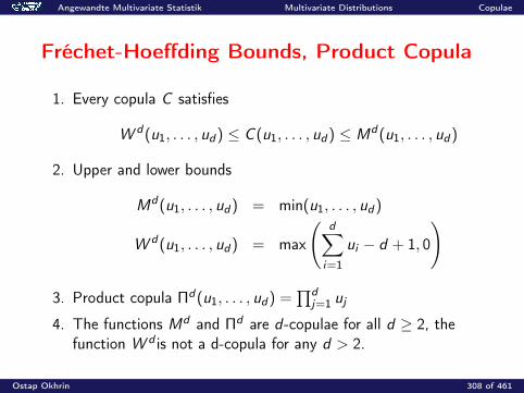
Angewandte Multivariate Statistik Multivariate Distributions Copulae
Fréchet-Hoeffding Bounds, Product Copula
1. Every copula C satisfies
W d(u1, . . . , ud) ≤ C (u1, . . . , ud) ≤ Md(u1, . . . , ud)
2. Upper and lower bounds
Md(u1, . . . , ud) = min(u1, . . . , ud)
W d(u1, . . . , ud) = max
(d∑
i=1
ui − d + 1, 0
)
3. Product copula Πd(u1, . . . , ud) =∏d
j=1 uj
4. The functions Md and Πd are d-copulae for all d ≥ 2, thefunction W d is not a d-copula for any d > 2.
Ostap Okhrin 308 of 461
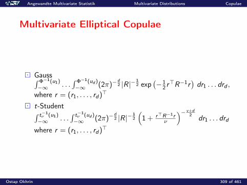
Angewandte Multivariate Statistik Multivariate Distributions Copulae
Multivariate Elliptical Copulae
Gauss∫ Φ−1(u1)−∞ . . .
∫ Φ−1(ud )−∞ (2π)−
d2 |R|−
12 exp
(−1
2 r>R−1r
)dr1 . . . drd ,
where r = (r1, . . . , rd)>
t-Student∫ t−1ν (u1)−∞ . . .
∫ t−1ν (ud )−∞ (2π)−
d2 |R|−
12
(1 + r>R−1r
ν
)− v+d2
dr1 . . . drd
where r = (r1, . . . , rd)>
Ostap Okhrin 309 of 461

Angewandte Multivariate Statistik Multivariate Distributions Copulae
Multivariate Archimedean Copulae
Gumbel
C (u1, . . . , ud) = exp[−
(− log u1)θ + . . .+ (− log ud)θ 1θ
] Cook-Johnson
C (u1, . . . , ud) =
d∑j=1
u−θj − d + 1
− 1θ
Frank
C (u1, . . . , ud) = −1θlog1 +
(e−θu1 − 1) . . . (e−θud − 1)
(e−θ − 1)d−1
Ostap Okhrin 310 of 461
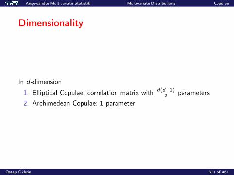
Angewandte Multivariate Statistik Multivariate Distributions Copulae
Dimensionality
In d-dimension1. Elliptical Copulae: correlation matrix with d(d−1)
2 parameters2. Archimedean Copulae: 1 parameter
Ostap Okhrin 311 of 461
Angewandte Multivariate Statistik Multivariate Distributions Copulae
Conclusions
Pluses of copulae flexible and wide range of dependence easy to simulate, estimate, implement explicit form of densities of copulae modelling of fat tails, assymetries
Minuses of copulae Elliptical: correlation matrix, symmetry Archimedean: too restrictive, single parameter, exchangable selection of copula
Ostap Okhrin 312 of 461

Angewandte Multivariate Statistik Theory of the Multinormal Elementary Properties
Theory of the Multinormal
Elementary Properties of the MultinormalThe pdf of X ∼ Np (µ,Σ) is given by:
f (x) = |2πΣ|−1/2 exp−12
(x − µ)>Σ−1(x − µ)
The expectation and variance are respectively given by:
E(X ) = µ,Var(X ) = Σ
Ostap Okhrin 313 of 461
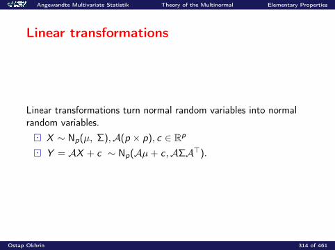
Angewandte Multivariate Statistik Theory of the Multinormal Elementary Properties
Linear transformations
Linear transformations turn normal random variables into normalrandom variables. X ∼ Np(µ, Σ),A(p × p), c ∈ Rp
Y = AX + c ∼ Np(Aµ+ c ,AΣA>).
Ostap Okhrin 314 of 461
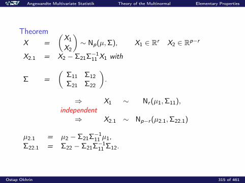
Angewandte Multivariate Statistik Theory of the Multinormal Elementary Properties
TheoremX =
(X1
X2
)∼ Np(µ,Σ), X1 ∈ Rr X2 ∈ Rp−r
X2.1 = X2 − Σ21Σ−111 X1 with
Σ =(
Σ11 Σ12Σ21 Σ22
).
⇒ X1 ∼ Nr (µ1,Σ11),independent
⇒ X2.1 ∼ Np−r (µ2.1,Σ22.1)
µ2.1 = µ2 − Σ21Σ−111 µ1,
Σ22.1 = Σ22 − Σ21Σ−111 Σ12.
Ostap Okhrin 315 of 461
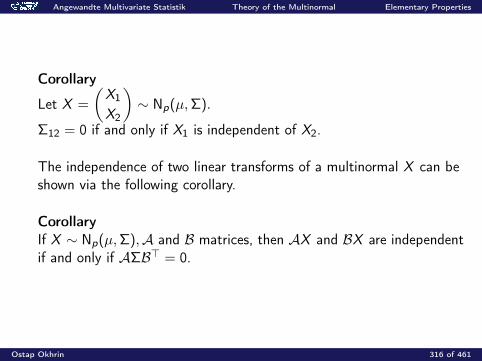
Angewandte Multivariate Statistik Theory of the Multinormal Elementary Properties
Corollary
Let X =
(X1
X2
)∼ Np(µ,Σ).
Σ12 = 0 if and only if X1 is independent of X2.
The independence of two linear transforms of a multinormal X can beshown via the following corollary.
CorollaryIf X ∼ Np(µ,Σ),A and B matrices, then AX and BX are independentif and only if AΣB> = 0.
Ostap Okhrin 316 of 461
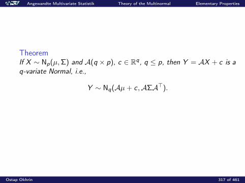
Angewandte Multivariate Statistik Theory of the Multinormal Elementary Properties
TheoremIf X ∼ Np(µ,Σ) and A(q × p), c ∈ Rq, q ≤ p, then Y = AX + c is aq-variate Normal, i.e.,
Y ∼ Nq(Aµ+ c ,AΣA>).
Ostap Okhrin 317 of 461
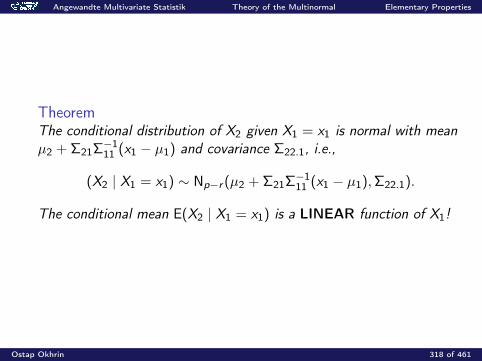
Angewandte Multivariate Statistik Theory of the Multinormal Elementary Properties
TheoremThe conditional distribution of X2 given X1 = x1 is normal with meanµ2 + Σ21Σ−1
11 (x1 − µ1) and covariance Σ22.1, i.e.,
(X2 | X1 = x1) ∼ Np−r (µ2 + Σ21Σ−111 (x1 − µ1),Σ22.1).
The conditional mean E(X2 | X1 = x1) is a LINEAR function of X1!
Ostap Okhrin 318 of 461
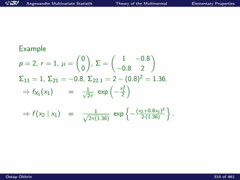
Angewandte Multivariate Statistik Theory of the Multinormal Elementary Properties
Example
p = 2, r = 1, µ =
(00
), Σ =
(1−0.8
−0.82
)Σ11 = 1, Σ21 = −0.8, Σ22.1 = 2− (0.8)2 = 1.36.
⇒ fX1(x1) = 1√2π
exp(− x21
2
)⇒ f (x2 | x1) = 1√
2π(1.36)exp− (x2+0.8x1)2
2·(1.36)
.
Ostap Okhrin 319 of 461
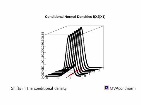
−10 −5 0 50.00
0.05
0.10
0.15
0.20
0.25
0.30
0.35
01
23
45
Conditional Normal Densities f(X2|X1)
Shifts in the conditional density. MVAcondnorm

Angewandte Multivariate Statistik Theory of the Multinormal Elementary Properties
TheoremIf X1 ∼ Nr (µ1,Σ11) and (X2|X1 = x1) ∼ Np−r (Ax1 + b,Ω) where Ωdoes not depend on x1, then
X =
(X1
X2
)∼ Np(µ,Σ),
where
µ =
(µ1
Aµ1 + b
)and
Σ =
(Σ11 Σ11A>AΣ11 Ω +AΣ11A>
).
Ostap Okhrin 321 of 461
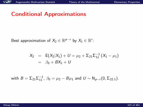
Angewandte Multivariate Statistik Theory of the Multinormal Elementary Properties
Conditional Approximations
Best approximation of X2 ∈ Rp−r by X1 ∈ Rr :
X2 = E(X2|X1) + U = µ2 + Σ21Σ−111 (X1 − µ1)
= β0 + BX1 + U
with B = Σ21Σ−111 , β0 = µ2 − Bµ1 and U ∼ Np−r (0,Σ22.1).
Ostap Okhrin 322 of 461

Angewandte Multivariate Statistik Theory of the Multinormal Elementary Properties
Consider the case where X2 ∈ R, i.e., r = p − 1.Now B is (1× r)-row vector β> such that:
X2 = β0 + β> X1 + U.
This means that the best MSE approximation of X2 by a function ofX1 is a hyperplane.
Ostap Okhrin 323 of 461
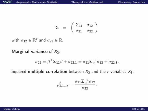
Angewandte Multivariate Statistik Theory of the Multinormal Elementary Properties
Σ =
(Σ11 σ12σ21 σ22
)with σ12 ∈ Rr and σ22 ∈ R.
Marginal variance of X2:
σ22 = β>Σ11β + σ22.1 = σ21Σ−111 σ12 + σ22.1.
Squared multiple correlation between X2 and the r variables X1:
ρ22.1...r =
σ21Σ−111 σ12
σ22.
Ostap Okhrin 324 of 461
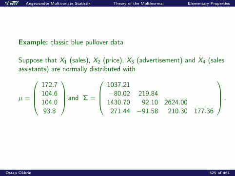
Angewandte Multivariate Statistik Theory of the Multinormal Elementary Properties
Example: classic blue pullover data
Suppose that X1 (sales), X2 (price), X3 (advertisement) and X4 (salesassistants) are normally distributed with
µ =
172.7104.6104.093.8
and Σ =
1037.21−80.02 219.841430.70 92.10 2624.00271.44 −91.58 210.30 177.36
.
Ostap Okhrin 325 of 461
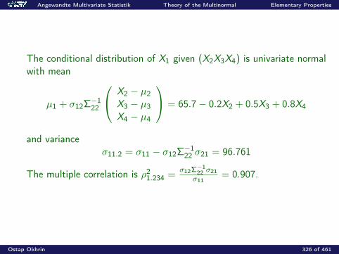
Angewandte Multivariate Statistik Theory of the Multinormal Elementary Properties
The conditional distribution of X1 given (X2X3X4) is univariate normalwith mean
µ1 + σ12Σ−122
X2 − µ2X3 − µ3X4 − µ4
= 65.7− 0.2X2 + 0.5X3 + 0.8X4
and varianceσ11.2 = σ11 − σ12Σ−1
22 σ21 = 96.761
The multiple correlation is ρ21.234 =
σ12Σ−122 σ21σ11
= 0.907.
Ostap Okhrin 326 of 461
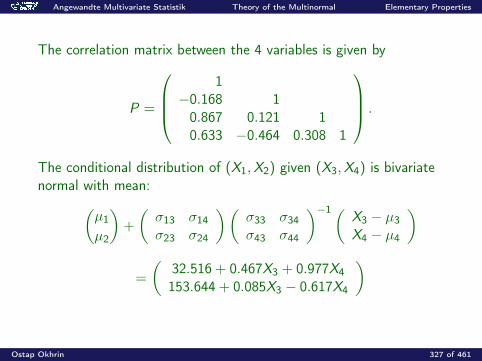
Angewandte Multivariate Statistik Theory of the Multinormal Elementary Properties
The correlation matrix between the 4 variables is given by
P =
1
−0.168 10.867 0.121 10.633 −0.464 0.308 1
.
The conditional distribution of (X1,X2) given (X3,X4) is bivariatenormal with mean:(
µ1
µ2
)+
(σ13 σ14σ23 σ24
)(σ33 σ34σ43 σ44
)−1(X3 − µ3X4 − µ4
)
=
(32.516 + 0.467X3 + 0.977X4153.644 + 0.085X3 − 0.617X4
)
Ostap Okhrin 327 of 461
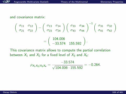
Angewandte Multivariate Statistik Theory of the Multinormal Elementary Properties
and covariance matrix:(σ11 σ12σ21 σ22
)−(σ13 σ14σ23 σ24
)(σ33 σ34σ43 σ44
)−1(σ31 σ32σ41 σ42
)
=
(104.006−33.574 155.592
).
This covariance matrix allows to compute the partial correlationbetween X1 and X2 for a fixed level of X3 and X4:
ρX1X2|X3X4 =−33.574√
104.006 · 155.592= −0.264.
Ostap Okhrin 328 of 461

Angewandte Multivariate Statistik Theory of the Multinormal Elementary Properties
Mahalanobis Transform
If X ∼ Np(µ,Σ) then the Mahalanobis transform is
Y = Σ−1/2(X − µ) ∼ Np(0, Ip)
and it holds
Y>Y = (X − µ)> Σ−1(X − µ) ∼ χ2p.
Y is random vector and Y>Y is scalar. Y>Y can be used for testing (assuming that Σ is known). Normally, we do not know Σ. The tests in this situation can be
carried out using Wishart and Hotelling distributions.
Ostap Okhrin 329 of 461

Angewandte Multivariate Statistik Theory of the Multinormal Elementary Properties
Summary: Elementary Properties
If X ∼ Np(µ,Σ) then a linear transformationAX + c ,A(q × p), c ∈ Rq has distribution Nq(Aµ+ c ,AΣA>).
Two linear transformations AX and BX of X ∼ Np(µ,Σ) areindependent if and only if AΣB> = 0.
If X1 and X2 are partitions of X ∼ Np(µ,Σ) then the conditionaldistribution of X2 given X1 = x1 is normal again.
Ostap Okhrin 330 of 461
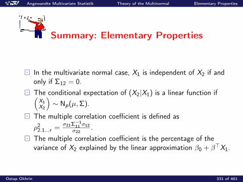
Angewandte Multivariate Statistik Theory of the Multinormal Elementary Properties
Summary: Elementary Properties
In the multivariate normal case, X1 is independent of X2 if andonly if Σ12 = 0.
The conditional expectation of (X2|X1) is a linear function if(X1X2
)∼ Np(µ,Σ).
The multiple correlation coefficient is defined asρ22.1...r =
σ21Σ−111 σ12σ22
.
The multiple correlation coefficient is the percentage of thevariance of X2 explained by the linear approximation β0 + β>X1.
Ostap Okhrin 331 of 461
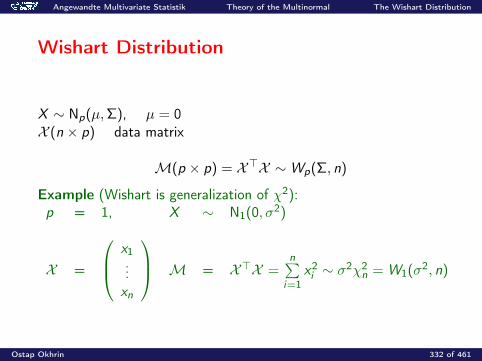
Angewandte Multivariate Statistik Theory of the Multinormal The Wishart Distribution
Wishart Distribution
X ∼ Np(µ,Σ), µ = 0X (n × p) data matrix
M(p × p) = X>X ∼Wp(Σ, n)
Example (Wishart is generalization of χ2):p = 1, X ∼ N1(0, σ2)
X =
x1...xn
M = X>X =n∑
i=1x2i ∼ σ2χ2
n = W1(σ2, n)
Ostap Okhrin 332 of 461
Angewandte Multivariate Statistik Theory of the Multinormal The Wishart Distribution
Linear Transformation of the Data Matrix
Theorem
M∼Wp(Σ, n), B(p × q)
⇒ B>MB ∼Wq(B>ΣB, n)
Ostap Okhrin 333 of 461
Angewandte Multivariate Statistik Theory of the Multinormal The Wishart Distribution
Wishart and χ2p- Distribution
Theorem
M∼Wp(Σ, n) , a ∈ Rp , a>Σa 6= 0
⇒ a>Ma
a>Σa∼ χ2
n
Ostap Okhrin 334 of 461
Angewandte Multivariate Statistik Theory of the Multinormal The Wishart Distribution
Theorem (Cochran)
X (n × p) data matrix from a Np(0,Σ) distribution
nS = X>HX ∼Wp(Σ, n − 1)S is the sample covariance matrix
x and S are independent
Ostap Okhrin 335 of 461
Angewandte Multivariate Statistik Theory of the Multinormal The Wishart Distribution
Summary: Wishart Distribution
The Wishart distribution is a generalization of the χ2-distribution.In particular W1(σ2, n) = σ2χ2
n. The empirical covariance matrix S has a 1
nWp(Σ, n − 1)distribution.
In the normal case, x and S are independent. ForM∼Wp(Σ,m), a>Ma
a>Σa∼ χ2
m.
Ostap Okhrin 336 of 461
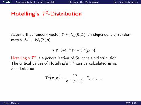
Angewandte Multivariate Statistik Theory of the Multinormal Hotelling Distribution
Hotelling’s T 2-Distribution
Assume that random vector Y ∼ Np(0, I) is independent of randommatrixM∼Wp(I, n).
n Y>M−1Y ∼ T 2(p, n)
Hotelling’s T 2 is a generalization of Student’s t-distributionThe critical values of Hotelling’s T 2 can be calculated usingF -distribution:
T 2(p, n) =np
n − p + 1Fp,n−p+1
Ostap Okhrin 337 of 461
Angewandte Multivariate Statistik Theory of the Multinormal Hotelling Distribution
Summary: Hotelling’s T 2-Distribution
Hotelling’s T 2-distribution is a generalization of thet-distribution. In particular T (1, n) = tn.
(n − 1)(x − µ)>S−1(x − µ) has a T 2(p, n − 1) distribution. The relation between Hotelling’s T 2− and Fisher’s F -distribution
is given by T 2(p, n) = npn−p+1 Fp,n−p+1.
Ostap Okhrin 338 of 461
Angewandte Multivariate Statistik Theory of Estimation The Likelihood Function
Theory of Estimation
In parametric statistics, θ is a k-variate vector θ ∈ Rk characterizingthe unknown properties of the population pdf f (x ; θ)
The aim will be to estimate θ from the sample X through estimators θwhich are functions of the sample: θ = θ(X ).
We must derive the sampling distribution of θ to analyze its properties(is it related to the unknown quantity θ it is supposed to estimate?).
We will utilise the maximum likelihood theory.
Ostap Okhrin 339 of 461
Angewandte Multivariate Statistik Theory of Estimation The Likelihood Function
The Likelihood Function
X ∼ f (x ; θ) pdf of an i.i.d. sample xini=1 with parameter θLikelihood function
L(X ; θ) =n∏
i=1
f (xi ; θ)
MLEθ = argmax
θL(X ; θ)
log-likelihood`(X ; θ) = log L(X ; θ)
Ostap Okhrin 340 of 461
Angewandte Multivariate Statistik Theory of Estimation The Likelihood Function
ExampleSample xini=1 from Np(µ, I), i.e. from the pdf
f (x ; θ) = (2π)−p/2 exp−12
(x − θ)>(x − θ)
where θ = µ ∈ Rp is the mean vector parameter.The log-likelihood is
`(X ; θ) =n∑
i=1
logf (xi ; θ) = log (2π)−np/2 − 12
n∑i=1
(xi − θ)>(xi − θ).
The term (xi − θ)>(xi − θ) equals
(xi − x)>(xi − x) + (x − θ)>(x − θ) + 2(x − θ)>(xi − x).
Ostap Okhrin 341 of 461
Angewandte Multivariate Statistik Theory of Estimation The Likelihood Function
ExampleIf we sum up this term over i = 1, . . . , n we see that
n∑i=1
(xi − θ)>(xi − θ) =n∑
i=1
(xi − x)>(xi − x) + n(x − θ)>(x − θ).
Hence
`(X ; θ) = log(2π)−np/2 − 12
n∑i=1
(xi − x)>(xi − x)− n
2(x − θ)>(x − θ).
Only the last term depends on θ and is obviously maximized for
θ = µ = x .
Thus x is the MLE.
Ostap Okhrin 342 of 461
Angewandte Multivariate Statistik Theory of Estimation The Likelihood Function
Example (MLE’s from a Normal Distribution)xini=1 is a sample from a normal distribution Np(µ,Σ)Due to the symmetry of Σ, the unknown parameter θ is in factp + 1
2p(p + 1)-dimensional.Then
L(X ; θ) = |2πΣ|−n/2 exp
−12
n∑i=1
(xi − µ)>Σ−1(xi − µ)
and
`(X ; θ) = −n
2log |2πΣ| − 1
2
n∑i=1
(xi − µ)>Σ−1(xi − µ).
Ostap Okhrin 343 of 461
Angewandte Multivariate Statistik Theory of Estimation The Likelihood Function
Example (MLE’s from a Normal Distribution - cont’d)The term (xi − µ)>Σ−1(xi − µ) equals
(xi − x)>Σ−1(xi − x) + (x − µ)>Σ−1(x − µ) + 2(x − µ)>Σ−1(xi − x).
If we sum up this term over i = 1, . . . , n we see that
n∑i=1
(xi − µ)>Σ−1(xi − µ)
=n∑
i=1
(xi − x)>Σ−1(xi − x) + n(x − µ)>Σ−1(x − µ).
Ostap Okhrin 344 of 461
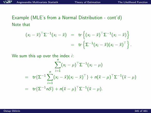
Angewandte Multivariate Statistik Theory of Estimation The Likelihood Function
Example (MLE’s from a Normal Distribution - cont’d)Note that
(xi − x)>Σ−1(xi − x) = tr
(xi − x)>Σ−1(xi − x)
= tr
Σ−1(xi − x)(xi − x)>.
We sum this up over the index i :n∑
i=1
(xi − µ)>Σ−1(xi − µ)
= trΣ−1n∑
i=1
(xi − x)(xi − x)>+ n(x − µ)>Σ−1(x − µ)
= trΣ−1nS+ n(x − µ)>Σ−1(x − µ).
Ostap Okhrin 345 of 461
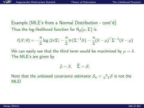
Angewandte Multivariate Statistik Theory of Estimation The Likelihood Function
Example (MLE’s from a Normal Distribution - cont’d)Thus the log-likelihood function for Np(µ,Σ) is
`(X ; θ) = −n
2log |2πΣ| − n
2trΣ−1S − n
2(x − µ)>Σ−1(x − µ)
We can easily see that the third term would be maximized by µ = x .The MLE’s are given by
µ = x , Σ = S.
Note that the unbiased covariance estimator Su = nn−1S is not the
MLE!
Ostap Okhrin 346 of 461
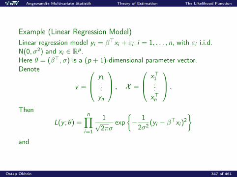
Angewandte Multivariate Statistik Theory of Estimation The Likelihood Function
Example (Linear Regression Model)Linear regression model yi = β>xi + εi ; i = 1, . . . , n, with εi i.i.d.N(0, σ2) and xi ∈ Rp.Here θ = (β>, σ) is a (p + 1)-dimensional parameter vector.Denote
y =
y1...yn
, X =
x>1...x>n
.
Then
L(y ; θ) =n∏
i=1
1√2πσ
exp− 12σ2 (yi − β>xi )2
and
Ostap Okhrin 347 of 461
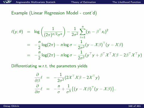
Angewandte Multivariate Statistik Theory of Estimation The Likelihood Function
Example (Linear Regression Model - cont’d)
`(y ; θ) = log(
1(2π)n/2σn
)− 1
2σ2
n∑i=1
(yi − β>xi )2
= −n
2log(2π)− n log σ − 1
2σ2 (y −Xβ)>(y −Xβ)
= −n
2log(2π)− n log σ − 1
2σ2 (y>y + β>X>Xβ − 2β>X>y)
Differentiating w.r.t. the parameters yields
∂
∂β` = − 1
2σ2 (2X>Xβ − 2X>y)
∂
∂σ` = −n
σ+
1σ3
(y −Xβ)>(y −Xβ)
.
Ostap Okhrin 348 of 461
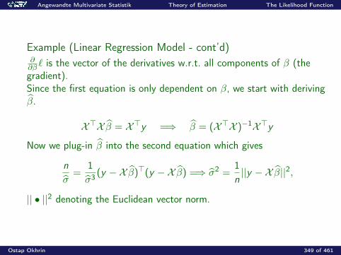
Angewandte Multivariate Statistik Theory of Estimation The Likelihood Function
Example (Linear Regression Model - cont’d)∂∂β ` is the vector of the derivatives w.r.t. all components of β (thegradient).Since the first equation is only dependent on β, we start with derivingβ.
X>X β = X>y =⇒ β = (X>X )−1X>y
Now we plug-in β into the second equation which gives
n
σ=
1σ3 (y −X β)>(y −X β) =⇒ σ2 =
1n||y −X β||2,
|| • ||2 denoting the Euclidean vector norm.
Ostap Okhrin 349 of 461
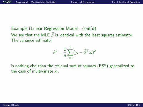
Angewandte Multivariate Statistik Theory of Estimation The Likelihood Function
Example (Linear Regression Model - cont’d)We see that the MLE β is identical with the least squares estimator.The variance estimator
σ2 =1n
n∑i=1
(yi − β>xi )2
is nothing else than the residual sum of squares (RSS) generalized tothe case of multivariate xi .
Ostap Okhrin 350 of 461
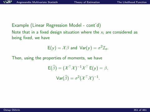
Angewandte Multivariate Statistik Theory of Estimation The Likelihood Function
Example (Linear Regression Model - cont’d)Note that in a fixed design situation where the xi are considered asbeing fixed, we have
E(y) = Xβ and Var(y) = σ2In.
Then, using the properties of moments, we have
E(β) = (X>X )−1X> E(y) = β,
Var(β) = σ2(X>X )−1.
Ostap Okhrin 351 of 461
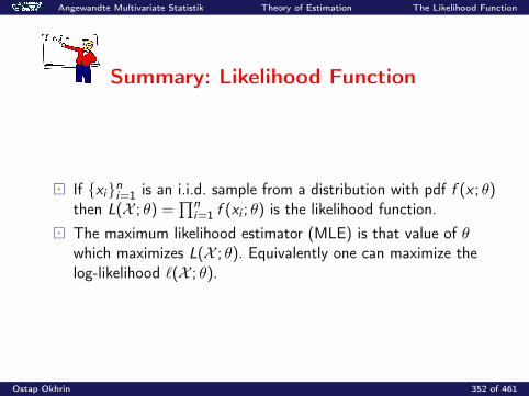
Angewandte Multivariate Statistik Theory of Estimation The Likelihood Function
Summary: Likelihood Function
If xini=1 is an i.i.d. sample from a distribution with pdf f (x ; θ)then L(X ; θ) =
∏ni=1 f (xi ; θ) is the likelihood function.
The maximum likelihood estimator (MLE) is that value of θwhich maximizes L(X ; θ). Equivalently one can maximize thelog-likelihood `(X ; θ).
Ostap Okhrin 352 of 461
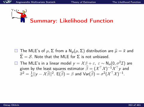
Angewandte Multivariate Statistik Theory of Estimation The Likelihood Function
Summary: Likelihood Function
The MLE’s of µ,Σ from a Np(µ,Σ) distribution are µ = x andΣ = S. Note that the MLE for Σ is not unbiased.
The MLE’s in a linear model y = Xβ + ε, ε ∼ Nn(0, σ2I) aregiven by the least squares estimator β = (X>X )−1X>y andσ2 = 1
n ||y −X β||2. E(β) = β and Var(β) = σ2(X>X )−1.
Ostap Okhrin 353 of 461
Angewandte Multivariate Statistik Theory of Estimation Cramer-Rao Lower Bound
Cramer-Rao Lower bound
One typical property we want for an estimator is unbiasedness: E(θ) = θ. (x is an unbiased estimator of µ and S is a biased
estimator of Σ in finite sample). We look for an unbiased estimator with the smallest possible
variance. The Cramer-Rao lower bound will achieve this and it provides the
asymptotic optimality property of maximum likelihood estimators. The Cramer-Rao theorem involves the score function and its
properties, which are first derived.
Ostap Okhrin 354 of 461

Angewandte Multivariate Statistik Theory of Estimation Cramer-Rao Lower Bound
Score Function and Fisher Information
The score function is
s(X ; θ) =∂
∂θ`(X ; θ)
The covariance matrix Fn = Vars(X ; θ) is called the Fisherinformation matrix.
Ostap Okhrin 355 of 461
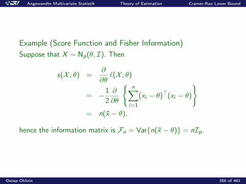
Angewandte Multivariate Statistik Theory of Estimation Cramer-Rao Lower Bound
Example (Score Function and Fisher Information)Suppose that X ∼ Np(θ, I). Then
s(X ; θ) =∂
∂θ`(X ; θ)
= −12∂
∂θ
n∑
i=1
(xi − θ)>(xi − θ)
= n(x − θ),
hence the information matrix is Fn = Varn(x − θ) = nIp.
Ostap Okhrin 356 of 461
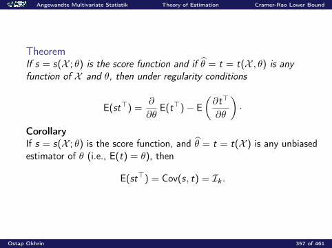
Angewandte Multivariate Statistik Theory of Estimation Cramer-Rao Lower Bound
TheoremIf s = s(X ; θ) is the score function and if θ = t = t(X , θ) is anyfunction of X and θ, then under regularity conditions
E(st>) =∂
∂θE(t>)− E
(∂t>
∂θ
)·
CorollaryIf s = s(X ; θ) is the score function, and θ = t = t(X ) is any unbiasedestimator of θ (i.e., E(t) = θ), then
E(st>) = Cov(s, t) = Ik .
Ostap Okhrin 357 of 461

Angewandte Multivariate Statistik Theory of Estimation Cramer-Rao Lower Bound
Note that the score function has mean zero
Es(X ; θ) = 0.
Hence, E(ss>) = Var(s) = Fn and it follows that
Fn = −E
∂2
∂θ∂θ>`(X ; θ)
.
RemarkIf x1, · · · , xn are i.i.d., Fn = nF1 where F1 is the Fisher informationmatrix for sample size n = 1.
Ostap Okhrin 358 of 461
Angewandte Multivariate Statistik Theory of Estimation Cramer-Rao Lower Bound
All estimators which are unbiased and attain the Cramer-Rao lowerbound are minimum variance estimators.
Theorem (Cramer-Rao)If θ = t = t(X ) is any unbiased estimator for θ then under regularityconditions
Var(t) ≥ F−1n ,
whereFn = Es(X ; θ)s(X ; θ)> = Vars(X ; θ)
is the Fisher information matrix
Ostap Okhrin 359 of 461
Angewandte Multivariate Statistik Theory of Estimation Cramer-Rao Lower Bound
Beweis.Consider the correlation ρY ,Z between Y and Z where Y = a>t,Z = c>s, and s is the score and the vectors a, c ∈ Rp. By theCorollary Cov(s, t) = I and thus
Cov(Y ,Z ) = a> Cov(t, s)c = a>c
Var(Z ) = c> Var(s)c = c>Fnc .
Hence,
ρ2Y ,Z =
Cov2(Y ,Z )
Var(Y )Var(Z )=
(a>c)2
a> Var(t)a· c>Fnc≤ 1.
Ostap Okhrin 360 of 461

Angewandte Multivariate Statistik Theory of Estimation Cramer-Rao Lower Bound
cont’d.In particular, this holds for any c 6= 0. Therefore it holds also for themaximum of the left-hand side with respect to c . Since
maxc
c>aa>c
c>Fnc= max
c>Fnc=1c>aa>c
andmax
c>Fnc=1c>aa>c = a>F−1
n a
Ostap Okhrin 361 of 461
Angewandte Multivariate Statistik Theory of Estimation Cramer-Rao Lower Bound
By the maximization theorem in the chapter on Matrix Algebra wehave
a>F−1n a
a> Var(t)a≤ 1 ∀ a ∈ Rp, a 6= 0,
i.e.,a>Var(t)−F−1
n a ≥ 0 ∀ a ∈ Rp, a 6= 0,
which is equivalent to Var(t) ≥ F−1n .
Ostap Okhrin 362 of 461
Angewandte Multivariate Statistik Theory of Estimation Cramer-Rao Lower Bound
Asymptotic Sampling Distribution of the MLE
Maximum likelihood estimators (MLE’s) attain the lower bound if thesample size n goes to infinity. The next theorem states this and, inaddition, gives the asymptotic sampling distribution of the maximumlikelihood estimation, which turns to be multinormal.
Ostap Okhrin 363 of 461
Angewandte Multivariate Statistik Theory of Estimation Cramer-Rao Lower Bound
TheoremSuppose that the sample xini=1 is i.i.d. If θ is the MLE for θ ∈ Rk ,i.e., θ = argmax
θL(X ; θ), then under some regularity conditions, as
n→∞: √n(θ − θ)
L−→ Nk(0,F−11 )
where F1 denotes the Fisher information for sample size n = 1.As a consequence we see that (under regularity conditions) the MLE isasymptotically unbiased, efficient (minimum variance) and normallydistributed.
Ostap Okhrin 364 of 461
Angewandte Multivariate Statistik Theory of Estimation Cramer-Rao Lower Bound
It follows that asymptotically
n(θ − θ)>F1(θ − θ)L→ χ2
p,
If F1 is a consistent estimator of F1
n(θ − θ)>F1(θ − θ)L→ χ2
p
This expression may be useful to test hypotheses about θ and toconstruct confidence regions for θ in a very general setup. It is clearthat
P(n(θ − θ)>F1(θ − θ) ≤ χ2
1−α;p
)≈ 1− α,
where χ2ν;p denotes the ν-quantile of a χ2
p random variable. So, theellipsoid n(θ − θ)>F1(θ − θ) ≤ χ2
1−α;p ∈ Rp provides an asymptotic(1− α)-confidence region for θ.
Ostap Okhrin 365 of 461

Angewandte Multivariate Statistik Theory of Estimation Cramer-Rao Lower Bound
Summary: Cramer-Rao Lower bound
The score function is the derivative s(X ; θ) = ∂∂θ`(X ; θ) of the
log-likelihood with respect to θ. The covariance matrix of s(X ; θ)is the Fisher information matrix.
Any unbiased estimator θ = t = t(X ) has a variance that isbounded below by the inverse of the Fisher information. Thus, anestimator, which attains this lower bound, is a minimal varianceestimator.
Ostap Okhrin 366 of 461
Angewandte Multivariate Statistik Theory of Estimation Cramer-Rao Lower Bound
Summary: Cramer-Rao Lower bound
MLE’s attain the lower bound in an asymptotic sense, i.e.,
√n(θ − θ)
L−→ N(0,F−11 )
if θ is the MLE θ = argmaxθ
L(X ; θ).
Ostap Okhrin 367 of 461
Angewandte Multivariate Statistik Hypothesis Testing Likelihood Ratio Test
Likelihood Ratio Test
Suppose that the distribution of xini=1, xi ∈ Rp, depends on aparameter vector θ. Then
H0 : θ ∈ Ω0
H1 : θ ∈ Ω1.
The hypothesis H0 corresponds to the “reduced model” and H1 to the“full model”.
Ostap Okhrin 368 of 461
Angewandte Multivariate Statistik Hypothesis Testing Likelihood Ratio Test
ExampleXi ∼ Np(θ, I)
H0 : θ = θ0
H1 : no constraints for θ
or equivalently to Ω0 = θ0, Ω1 = Rp.
Ostap Okhrin 369 of 461
Angewandte Multivariate Statistik Hypothesis Testing Likelihood Ratio Test
Likelihood RatioDefine L∗j = max
θ∈Ωj
L(X ; θ), the maxima of the likelihood for each of the
hypotheses.
λ(X ) =L∗0L∗1
Likelihood Ratio Testrejection region:
R = x : λ(x) < c
supθ∈Ω0
Pθ(x ∈ R) = α
Ostap Okhrin 370 of 461
Angewandte Multivariate Statistik Hypothesis Testing Likelihood Ratio Test
Theorem (Wilks)If Ω1 ⊂ Rq is a q-dimensional space and if Ω0 ⊂ Ω1 is anr -dimensional subspace, then under regularity conditions for n→∞
∀ θ ∈ Ω0 : −2 log λ L−→ χ2q−r .
Ostap Okhrin 371 of 461

Angewandte Multivariate Statistik Hypothesis Testing Likelihood Ratio Test
Test problem 1
X1, . . . ,Xn, i.i.d. with Xi ∼ Np(µ,Σ)
H0 : µ = µ0, Σ known, H1 : no constraints.
Ω0 = µ0, r = 0,Ω1 = Rp, q = p
−2 log λ = 2(`∗1 − `∗0) = n(x − µ0)>Σ−1(x − µ0)
−2 log λ ∼ χ2p
Rejection region R : x ∈ Rn such that −2 log λ > χ20.95;p
Ostap Okhrin 372 of 461
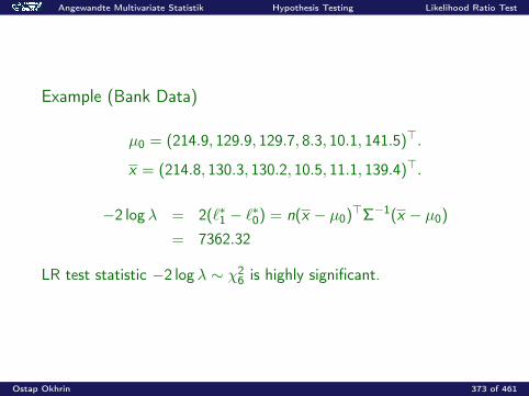
Angewandte Multivariate Statistik Hypothesis Testing Likelihood Ratio Test
Example (Bank Data)
µ0 = (214.9, 129.9, 129.7, 8.3, 10.1, 141.5)>.
x = (214.8, 130.3, 130.2, 10.5, 11.1, 139.4)>.
−2 log λ = 2(`∗1 − `∗0) = n(x − µ0)>Σ−1(x − µ0)
= 7362.32
LR test statistic −2 log λ ∼ χ26 is highly significant.
Ostap Okhrin 373 of 461

Angewandte Multivariate Statistik Hypothesis Testing Likelihood Ratio Test
Test problem 2Xi ∼ Np(µ,Σ) i.i.d.
H0 : µ = µ0, Σ unknown, H1 : no constraints.
Under H0 it can be shown that
`∗0 = `(µ0,S + dd>), d = (x − µ0)
and under H1 we have`∗1 = `(x ,S).
This leads to
− 2 log λ = 2(`∗1 − `∗0) = n log(1 + d>S−1d). (16)
Ostap Okhrin 374 of 461
Angewandte Multivariate Statistik Hypothesis Testing Likelihood Ratio Test
Test problem 2 cont’dNote that this statistic depends on (n − 1)d>S−1d which has, underH0, a Hotelling’s T 2-distribution. Therefore,
(n − 1)(x − µ0)>S−1(x − µ0) ∼ T 2(p, n − 1). (17)
or equivalently(n − p
p
)(x − µ0)>S−1(x − µ0) ∼ Fp,n−p
So the rejection region may be defined as(n − p
p
)(x − µ0)>S−1(x − µ0) > F1−α;p,n−p.
Ostap Okhrin 375 of 461
Angewandte Multivariate Statistik Hypothesis Testing Likelihood Ratio Test
Test problem 2 cont’dAlternatively we have, under H0, the asymptotic distribution
−2 log λ −→ χ2p,
leading to the rejection region
n log1 + (x − µ0)>S−1(x − µ0)
> χ2
1−α;p
Ostap Okhrin 376 of 461
Angewandte Multivariate Statistik Hypothesis Testing Likelihood Ratio Test
Confidence region for µ
(n−pp
)(x − µ)>S−1(x − µ) ∼ Fp,n−pµ ∈ Rp | (µ− x)>S−1(µ− x) ≤ p
n − pF1−α;p,n−p
is a confidence region at level (1-α) for µ; it is the interior of aniso-distance ellipsoid in Rp.When p is large, ellipsoids are difficult to practically handle. One isthus interested in finding confidence intervals for µ1, µ2, . . . , µp sothat simultaneous confidence on all the intervals reaches the desiredlevel say, 1− α.
Ostap Okhrin 377 of 461
Angewandte Multivariate Statistik Hypothesis Testing Likelihood Ratio Test
Simultaneous Confidence Intervals for a>µ
Obvious confidence interval for certain a>µ is given by:∣∣∣∣√n − 1(a>µ− a>x)√a>Sa
∣∣∣∣ ≤ t1−α2 ;n−1
or equivalently
t2(a) =(n − 1)
a>(µ− x)
2
a>Sa≤ F1−α;1,n−1
which provides the (1− α) confidence interval for a>µ:a>x −
√F1−α;1,n−1
a>San − 1
≤ a>µ ≤ a>x +
√F1−α;1,n−1
a>San − 1
.
Ostap Okhrin 378 of 461
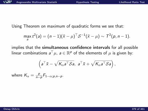
Angewandte Multivariate Statistik Hypothesis Testing Likelihood Ratio Test
Using Theorem on maximum of quadratic forms we see that:
maxa
t2(a) = (n − 1)(x − µ)>S−1(x − µ) ∼ T 2(p, n − 1).
implies that the simultaneous confidence intervals for all possiblelinear combinations a>µ, a ∈ Rp of the elements of µ is given by:(
a>x −√Kαa>Sa, a>x +
√Kαa>Sa
),
where Kα = pn−pF1−α;p,n−p.
Ostap Okhrin 379 of 461
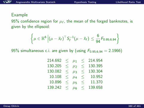
Angewandte Multivariate Statistik Hypothesis Testing Likelihood Ratio Test
Example95% confidence region for µf , the mean of the forged banknotes, isgiven by the ellipsoid:
µ ∈ R6∣∣∣(µ− xf )>S−1
f (µ− xf ) ≤ 694
F0.95;6,94
95% simultaneous c.i. are given by (using F0.95;6,94 = 2.1966)
214.692 ≤ µ1 ≤ 214.954130.205 ≤ µ2 ≤ 130.395130.082 ≤ µ3 ≤ 130.30410.108 ≤ µ4 ≤ 10.95210.896 ≤ µ5 ≤ 11.370
139.242 ≤ µ6 ≤ 139.658
Ostap Okhrin 380 of 461
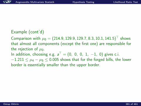
Angewandte Multivariate Statistik Hypothesis Testing Likelihood Ratio Test
Example (cont’d)Comparison with µ0 = (214.9, 129.9, 129.7, 8.3, 10.1, 141.5)> showsthat almost all components (except the first one) are responsible forthe rejection of µ0.In addition, choosing e.g. a> = (0, 0, 0, 1, −1, 0) gives c.i.−1.211 ≤ µ4 − µ5 ≤ 0.005 shows that for the forged bills, the lowerborder is essentially smaller than the upper border.
Ostap Okhrin 381 of 461
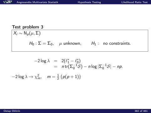
Angewandte Multivariate Statistik Hypothesis Testing Likelihood Ratio Test
Test problem 3Xi ∼ Np(µ,Σ)
H0 : Σ = Σ0, µ unknown, H1 : no constraints.
−2 log λ = 2(`∗1 − `∗0)= n tr(Σ−1
0 S)− n log |Σ−10 S| − np.
−2 log λ→ χ2m, m = 1
2 p(p + 1)
Ostap Okhrin 382 of 461
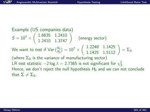
Angewandte Multivariate Statistik Hypothesis Testing Likelihood Ratio Test
Example (US companies data)
S = 107 ×(
1.6635 1.24101.2410 1.3747
)(energy sector)
We want to test if Var(X1X2
)= 107 ×
(1.2248 1.14251.1425 1.5112
)= Σ0
(where Σ0 is the variance of manufacturing sector)LR test statistic −2 log λ = 2.7365 is not significant for χ2
3.Hence, we don’t reject the null hypothesis H0 and we can not concludethat Σ 6= Σ0.
Ostap Okhrin 383 of 461
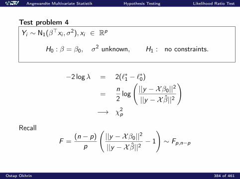
Angewandte Multivariate Statistik Hypothesis Testing Likelihood Ratio Test
Test problem 4Yi ∼ N1(β>xi , σ
2), xi ∈ Rp
H0 : β = β0, σ2 unknown, H1 : no constraints.
−2 log λ = 2(`∗1 − `∗0)
=n
2log
(||y −Xβ0||2
||y −X β||2
)−→ χ2
p
Recall
F =(n − p)
p
(||y −Xβ0||2
||y −X β||2− 1
)∼ Fp,n−p
Ostap Okhrin 384 of 461
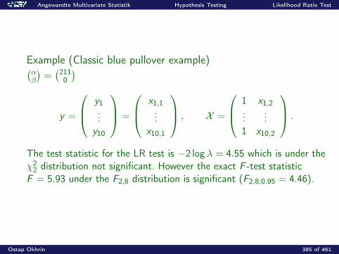
Angewandte Multivariate Statistik Hypothesis Testing Likelihood Ratio Test
Example (Classic blue pullover example)(αβ
)=(211
0
)
y =
y1...
y10
=
x1,1...
x10,1
, X =
1 x1,2...
...1 x10,2
.
The test statistic for the LR test is −2 log λ = 4.55 which is under theχ2
2 distribution not significant. However the exact F -test statisticF = 5.93 under the F2,8 distribution is significant (F2,8;0.95 = 4.46).
Ostap Okhrin 385 of 461
Angewandte Multivariate Statistik Hypothesis Testing Likelihood Ratio Test
Summary: Hypothesis Testing
The hypotheses H0 : θ ∈ Ω0 against H1 : θ ∈ Ω1 can be test bymeans of the likelihood ratio test (LRT).
The likelihood ratio (LR) is the quotient λ(X ) = L∗0/L∗1 where the
L∗j are the maxima of the likelihood in each of the hypotheses. The test statistic in the LRT is λ(X ) or equivalently its logarithm
log λ(X ).
Ostap Okhrin 386 of 461
Angewandte Multivariate Statistik Hypothesis Testing Likelihood Ratio Test
Summary: Hypothesis Testing
If Ω1 is q-dimensional and Ω0 ⊂ Ω1 r -dimensional, then theasymptotic distribution of −2 log λ is χ2
q−r . This allows to test H0against H1 by calculating as test statistic −2 log λ = 2(`∗1 − `∗0)where `∗j = log L∗j .
The hypothesis H0 : µ = µ0 for X ∼ Np(µ,Σ), Σ known, leads to−2 log λ = n(x − µ0)>Σ−1(x − µ0) ∼ χ2
p.
The hypothesis H0 : µ = µ0 for X ∼ Np(µ,Σ), Σ unknown, leadsto −2 log λ = n log1 + (x − µ0)>S−1(x − µ0) −→ χ2
p, and
(n − 1)(x − µ0)>S−1(x − µ0) ∼ T 2(p, n − 1).
Ostap Okhrin 387 of 461
Angewandte Multivariate Statistik Hypothesis Testing Likelihood Ratio Test
Summary: Hypothesis Testing
The hypothesis H0 : Σ = Σ0 for X ∼ Np(µ,Σ), µ unknown, leadsto −2 log λ = n tr
(Σ−1
0 S)− n log |Σ−1
0 S| − np −→ χ2m, m =
12p(p + 1).
The hypothesis H0 : β = β0 for Yi ∼ N1(β>xi , σ2), σ2 unknown,
leads to −2 log λ = n2 log
(||y−Xβ0||2
||y−X β||2
)−→ χ2
p.
Ostap Okhrin 388 of 461
Angewandte Multivariate Statistik Hypothesis Testing Linear Hypothesis
Linear Hypothesis
We present a general procedure which allows a linear hypothesis to betested.Linear hypotheses are of the form Aµ = a with known matricesA(q × p) and a(q × 1) with q ≤ p.
ExampleSuppose that X1 ∼ N(µ1, σ) and X2 ∼ N(µ2, σ) are independent andthat you want to test the hypothesis H0 : µ1 = µ2This can be written as linear hypothesis
H0 : Aµ =(1 −1
)( µ1µ2
)= 0.
Ostap Okhrin 389 of 461

Angewandte Multivariate Statistik Hypothesis Testing Linear Hypothesis
Test problem 5Xi ∼ Np(µ,Σ)
H0 : Aµ = a, Σ known, H1 : no constraints.
The results of the Test Problems 1 and 2 can directly be used on µy ,the mean of Yi = AXi .Indeed Yi ∼ Nq(µy ,Σy ) where µy=Aµ and Σy = AΣA>.Accordingly we have: y = Ax , Sy = ASA>, d = Ax − a.
n(Ax − a)>(AΣA>)−1(Ax − a) ∼ X 2q
Ostap Okhrin 390 of 461
Angewandte Multivariate Statistik Hypothesis Testing Linear Hypothesis
ExampleWe consider hypotheses on partitioned µ =
(µ1µ2
).
H0 : µ1 = µ2, H1 : no constraints,
for N2p((µ1µ2
),(
Σ0
0Σ
)) with known Σ.
This is equivalent to A = (Ip,−Ip), a = (0, . . . , 0︸ ︷︷ ︸p
)> and leads to
−2 log λ = n(x1 − x2)(2Σ)−1(x1 − x2) ∼ χ2p.
Ostap Okhrin 391 of 461

Angewandte Multivariate Statistik Hypothesis Testing Linear Hypothesis
ExampleAnother example is the test whether µ1 = 0, i.e.
H0 : µ1 = 0, H1 : no constraints,
for N2p((µ1µ2
),(
Σ0
0Σ
)) with known Σ.
This is equivalent to Aµ = a with A = (I, 0),a = (0, . . . , 0︸ ︷︷ ︸
p
)>.
Hence−2 log λ = nx1Σ−1x1 ∼ χ2
p.
Ostap Okhrin 392 of 461

Angewandte Multivariate Statistik Hypothesis Testing Linear Hypothesis
Test problem 6Xi ∼ Np(µ,Σ)
H0 : Aµ = a, Σ unknown, H1 : no constraints.
Ostap Okhrin 393 of 461
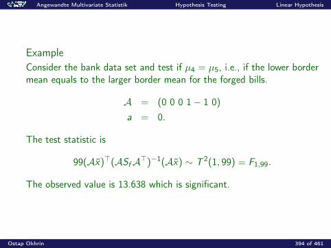
Angewandte Multivariate Statistik Hypothesis Testing Linear Hypothesis
ExampleConsider the bank data set and test if µ4 = µ5, i.e., if the lower bordermean equals to the larger border mean for the forged bills.
A = (0 0 0 1− 1 0)
a = 0.
The test statistic is
99(Ax)>(ASfA>)−1(Ax) ∼ T 2(1, 99) = F1,99.
The observed value is 13.638 which is significant.
Ostap Okhrin 394 of 461
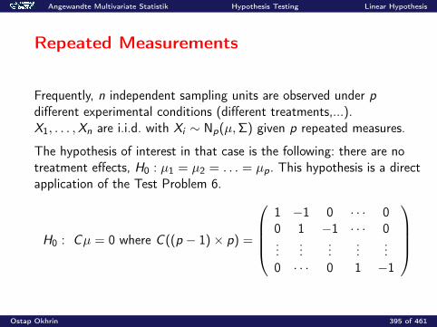
Angewandte Multivariate Statistik Hypothesis Testing Linear Hypothesis
Repeated Measurements
Frequently, n independent sampling units are observed under pdifferent experimental conditions (different treatments,...).X1, . . . ,Xn are i.i.d. with Xi ∼ Np(µ,Σ) given p repeated measures.
The hypothesis of interest in that case is the following: there are notreatment effects, H0 : µ1 = µ2 = . . . = µp. This hypothesis is a directapplication of the Test Problem 6.
H0 : Cµ = 0 where C ((p − 1)× p) =
1 −1 0 · · · 00 1 −1 · · · 0...
......
......
0 · · · 0 1 −1
Ostap Okhrin 395 of 461
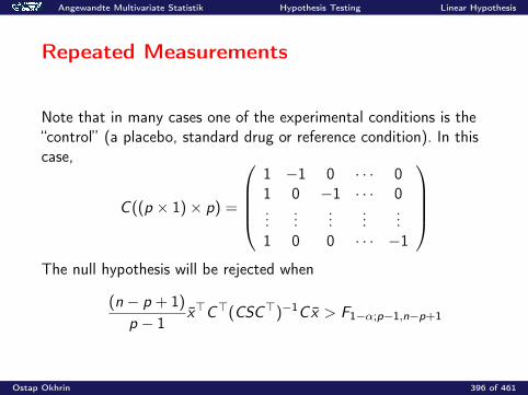
Angewandte Multivariate Statistik Hypothesis Testing Linear Hypothesis
Repeated Measurements
Note that in many cases one of the experimental conditions is the“control” (a placebo, standard drug or reference condition). In thiscase,
C ((p × 1)× p) =
1 −1 0 · · · 01 0 −1 · · · 0...
......
......
1 0 0 · · · −1
The null hypothesis will be rejected when
(n − p + 1)
p − 1x>C>(CSC>)−1Cx > F1−α;p−1,n−p+1
Ostap Okhrin 396 of 461
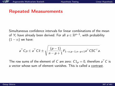
Angewandte Multivariate Statistik Hypothesis Testing Linear Hypothesis
Repeated Measurements
Simultaneous confidence intervals for linear combinations of the meanof Yi have already been derived. For all a ∈ Rp−1, with probability(1− α) we have:
a>Cµ ∈ a>Cx ±
√(p − 1)
n − p + 1F1−α;p−1,n−p+1a>CSC>a.
The row sums of the element of C are zero: C1p = 0, therefore a>C isa vector whose sum of element vanishes. This is called a contrast.
Ostap Okhrin 397 of 461
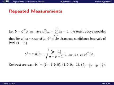
Angewandte Multivariate Statistik Hypothesis Testing Linear Hypothesis
Repeated Measurements
Let b = C>a, we have b>1p =p∑
j=1bj = 0, the result above provides
thus for all contrasts of µ, b>µ simultaneous confidence intervals oflevel (1− α)
b>µ ∈ b>x ±
√(p − 1)
n − p + 1F1−α;p−1,n−p+1b>Sb.
Contrast are e.g.: b> = (1,−1, 0, 0), (1, 0, 0,−1), (13 ,−
13 ,−
13 ,−
13).
Ostap Okhrin 398 of 461
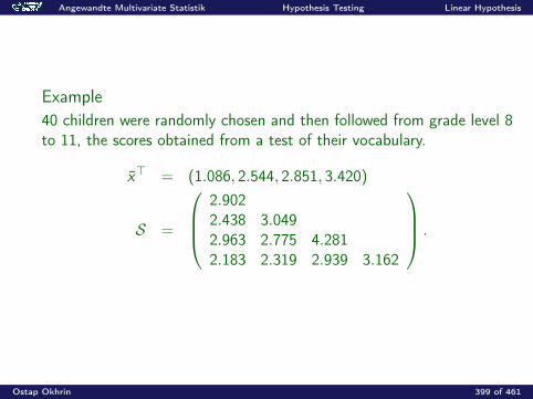
Angewandte Multivariate Statistik Hypothesis Testing Linear Hypothesis
Example40 children were randomly chosen and then followed from grade level 8to 11, the scores obtained from a test of their vocabulary.
x> = (1.086, 2.544, 2.851, 3.420)
S =
2.9022.438 3.0492.963 2.775 4.2812.183 2.319 2.939 3.162
.
Ostap Okhrin 399 of 461
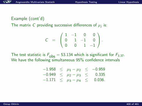
Angewandte Multivariate Statistik Hypothesis Testing Linear Hypothesis
Example (cont’d)The matrix C providing successive differences of µj is:
C =
1 −1 0 00 1 −1 00 0 1 −1
.
The test statistic is Fobs = 53.134 which is significant for F3.37.We have the following simultaneous 95% confidence intervals
−1.958 ≤ µ1 − µ2 ≤ −0.959−0.949 ≤ µ2 − µ3 ≤ 0.335−1.171 ≤ µ3 − µ4 ≤ 0.036.
Ostap Okhrin 400 of 461
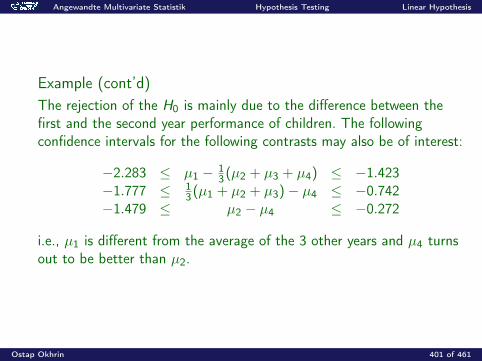
Angewandte Multivariate Statistik Hypothesis Testing Linear Hypothesis
Example (cont’d)The rejection of the H0 is mainly due to the difference between thefirst and the second year performance of children. The followingconfidence intervals for the following contrasts may also be of interest:
−2.283 ≤ µ1 − 13(µ2 + µ3 + µ4) ≤ −1.423
−1.777 ≤ 13(µ1 + µ2 + µ3)− µ4 ≤ −0.742
−1.479 ≤ µ2 − µ4 ≤ −0.272
i.e., µ1 is different from the average of the 3 other years and µ4 turnsout to be better than µ2.
Ostap Okhrin 401 of 461
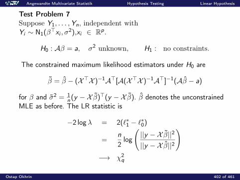
Angewandte Multivariate Statistik Hypothesis Testing Linear Hypothesis
Test Problem 7Suppose Y1, . . . ,Yn, independent withYi ∼ N1(β>xi , σ
2),xi ∈ Rp.
H0 : Aβ = a, σ2 unknown, H1 : no constraints.
The constrained maximum likelihood estimators under H0 are
β = β − (X>X )−1A>[A(X>X )−1A>]−1(Aβ − a)
for β and σ2 = 1n (y −X β)>(y −X β). β denotes the unconstrained
MLE as before. The LR statistic is
−2 log λ = 2(`∗1 − `∗0)
=n
2log
(||y −X β||2
||y −X β||2
)−→ χ2
q
Ostap Okhrin 402 of 461
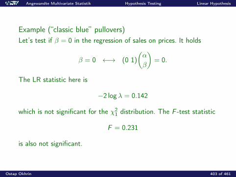
Angewandte Multivariate Statistik Hypothesis Testing Linear Hypothesis
Example (“classic blue” pullovers)Let’s test if β = 0 in the regression of sales on prices. It holds
β = 0 ←→ (0 1)
(α
β
)= 0.
The LR statistic here is
−2 log λ = 0.142
which is not significant for the χ21 distribution. The F -test statistic
F = 0.231
is also not significant.
Ostap Okhrin 403 of 461
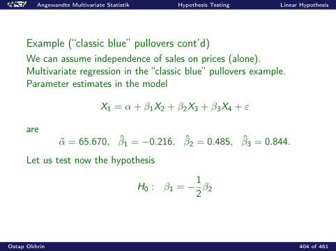
Angewandte Multivariate Statistik Hypothesis Testing Linear Hypothesis
Example (“classic blue” pullovers cont’d)We can assume independence of sales on prices (alone).Multivariate regression in the “classic blue” pullovers example.Parameter estimates in the model
X1 = α + β1X2 + β2X3 + β3X4 + ε
areα = 65.670, β1 = −0.216, β2 = 0.485, β3 = 0.844.
Let us test now the hypothesis
H0 : β1 = −12β2
Ostap Okhrin 404 of 461
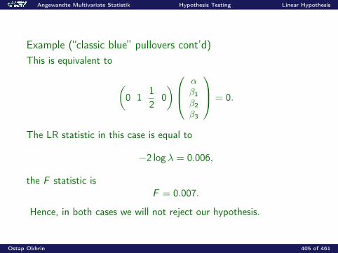
Angewandte Multivariate Statistik Hypothesis Testing Linear Hypothesis
Example (“classic blue” pullovers cont’d)This is equivalent to
(0 1
12
0) α
β1β2β3
= 0.
The LR statistic in this case is equal to
−2 log λ = 0.006,
the F statistic isF = 0.007.
Hence, in both cases we will not reject our hypothesis.
Ostap Okhrin 405 of 461
Angewandte Multivariate Statistik Hypothesis Testing Linear Hypothesis
Test Problem 8 (Comparison of two means)Suppose Xi1 ∼ Np(µ1,Σ),i = 1, · · · , n1 andXj2 ∼ Np(µ2,Σ),j = 1, · · · , n2, all the variables being independent.
H0 : µ1 = µ2, H1 : no constraints.
Both samples provide the statistics xk and Sk , k=1,2. Letδ = µ1 − µ2,we have
(x1 − x2) ∼ Np
(δ,n1 + n2
n1n2Σ
)n1S1 + n2S2 ∼Wp(Σ, n1 + n2 − 2).
Ostap Okhrin 406 of 461
Angewandte Multivariate Statistik Hypothesis Testing Linear Hypothesis
The rejection region will thus be given by:
n1n2(n1 + n2 − p − 1)
p(n1 + n2)2 ((x1 − x2))> S−1 ((x1 − x2))
≥ F1−α;p,n1+n2−p−1
A (1− α) ∗ 100% confidence region for δ is given by the ellipsoidcentered at (x1 − x2)
(δ − (x1 − x2))> S−1 (δ − (x1 − x2))
≤ p(n1 + n2)2
(n1 + n2 − p − 1)(n1n2)F1−α;p,n1+n2−p−1,
and the simultaneous confidence intervals for all linear combinations ofthe elements of δ : a>δ are given by
a>δ ∈ a>(x1−x2)±
√p(n1 + n2)2
(n1 + n2 − p − 1)(n1n2)F1−α;p,n1+n2−p−1a>Sa.
Ostap Okhrin 407 of 461
Angewandte Multivariate Statistik Hypothesis Testing Linear Hypothesis
ExampleWe want to compare the mean of the assets (X1) and of the sales (X2)of the two sectors energy (group 1) and manufacturing (group 2). Wehave the following statistics n1 = 15, n2 = 10, p = 2,
x1 =
(40842580.5
), x1 =
(4307.24925.2
)and
S1 = 107 ∗(
1.6635 1.24101.2410 1.3747
),
S2 = 107 ∗(
1.2248 1.14251.1425 1.5112
),
so that S = 107 ∗(
1.4880 1.20161.2016 1.4293
).
Ostap Okhrin 408 of 461
Angewandte Multivariate Statistik Hypothesis Testing Linear Hypothesis
ExampleThe observed value of the test statistic is Fobs = 2.7036. SinceF0.95;2,22 = 3.4434 the hypothesis of equal means of the two groups isnot rejected although it would be rejected at a less severe level(p − value = 0.0892). The 95% simultaneous confidence intervals forthe differences are given by
−4628.6 ≤ µ1a − µ2a ≤ 4182.2−6662.4 ≤ µ1s − µ2s ≤ 1973.0.
Ostap Okhrin 409 of 461
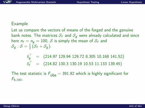
Angewandte Multivariate Statistik Hypothesis Testing Linear Hypothesis
ExampleLet us compare the vectors of means of the forged and the genuinebank notes. The matrices Sf and Sg were already calculated and sincehere nf = ng = 100, S is simply the mean of Sf andSg : S = 1
2 (Sf + Sg ).
x>g = (214.97 129.94 129.72 8.305 10.168 141.52)
x>f = (214.82 130.3 130.19 10.53 11.133 139.45)
The test statistic is Fobs = 391.92 which is highly significant forF6,193.
Ostap Okhrin 410 of 461
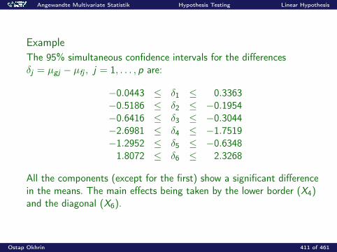
Angewandte Multivariate Statistik Hypothesis Testing Linear Hypothesis
ExampleThe 95% simultaneous confidence intervals for the differencesδj = µgj − µfj , j = 1, . . . , p are:
−0.0443 ≤ δ1 ≤ 0.3363−0.5186 ≤ δ2 ≤ −0.1954−0.6416 ≤ δ3 ≤ −0.3044−2.6981 ≤ δ4 ≤ −1.7519−1.2952 ≤ δ5 ≤ −0.63481.8072 ≤ δ6 ≤ 2.3268
All the components (except for the first) show a significant differencein the means. The main effects being taken by the lower border (X4)and the diagonal (X6).
Ostap Okhrin 411 of 461

Angewandte Multivariate Statistik Hypothesis Testing Linear Hypothesis
Test Problem 9 (Comparison of Covariance Matrices)Let Xih ∼ Np(µh,Σh), i = 1 · · · ,Nh; h = 1, · · · , kall variables being independent,
H0 : Σ1 = Σ2 = · · · = Σk , H1 : no constraints.
Ostap Okhrin 412 of 461
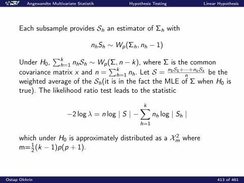
Angewandte Multivariate Statistik Hypothesis Testing Linear Hypothesis
Each subsample provides Sh an estimator of Σh with
nhSh ∼Wp(Σh, nh − 1)
Under H0,∑k
h=1 nhSh ∼Wp(Σ, n − k), where Σ is the commoncovariance matrix x and n =
∑kh=1 nh. Let S = n1S1+···+nkSk
n be theweighted average of the Sh(it is in the fact the MLE of Σ when H0 istrue). The likelihood ratio test leads to the statistic
−2 log λ = n log | S | −k∑
h=1
nh log | Sh |
which under H0 is approximately distributed as a X 2m where
m=12(k − 1)p(p + 1).
Ostap Okhrin 413 of 461

Angewandte Multivariate Statistik Hypothesis Testing Linear Hypothesis
ExampleCome back to US companies data, where the mean of assets and saleshave been compared for companies from the energy and manufacturingsector. The test Σ1 = Σ2 leads to the value of the test statistic
−2 log λ = 0.9076
which is not significant (p-value for a χ23 = 0.82). We cannot reject H0
and the comparison of the means above is valid.
Ostap Okhrin 414 of 461

Angewandte Multivariate Statistik Hypothesis Testing Linear Hypothesis
Test Problem 10 (Comparison of two means, unequal covariancematrices, large samples)Suppose Xi1 ∼ Np(µ1,Σ1),i = 1, · · · , n1 andXj2 ∼ Np(µ2,Σ2),j = 1, · · · , n2, all the variables being independent.
H0 : µ1 = µ2, H1 : no constraints.
Ostap Okhrin 415 of 461
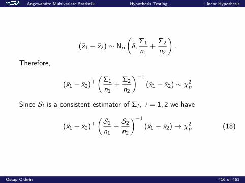
Angewandte Multivariate Statistik Hypothesis Testing Linear Hypothesis
(x1 − x2) ∼ Np
(δ,
Σ1
n1+
Σ2
n2
).
Therefore,
(x1 − x2)>(
Σ1
n1+
Σ2
n2
)−1
(x1 − x2) ∼ χ2p
Since Si is a consistent estimator of Σi , i = 1, 2 we have
(x1 − x2)>(S1
n1+S2
n2
)−1
(x1 − x2)→ χ2p (18)
Ostap Okhrin 416 of 461
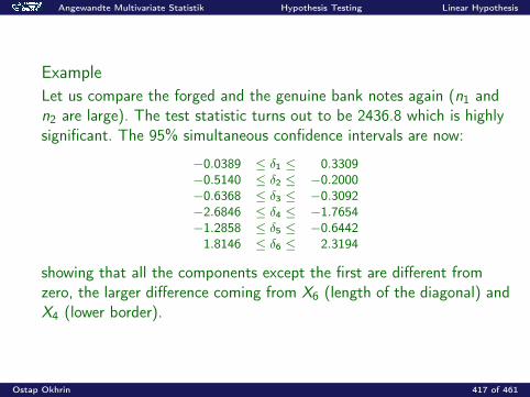
Angewandte Multivariate Statistik Hypothesis Testing Linear Hypothesis
ExampleLet us compare the forged and the genuine bank notes again (n1 andn2 are large). The test statistic turns out to be 2436.8 which is highlysignificant. The 95% simultaneous confidence intervals are now:
−0.0389 ≤ δ1 ≤ 0.3309−0.5140 ≤ δ2 ≤ −0.2000−0.6368 ≤ δ3 ≤ −0.3092−2.6846 ≤ δ4 ≤ −1.7654−1.2858 ≤ δ5 ≤ −0.6442
1.8146 ≤ δ6 ≤ 2.3194
showing that all the components except the first are different fromzero, the larger difference coming from X6 (length of the diagonal) andX4 (lower border).
Ostap Okhrin 417 of 461
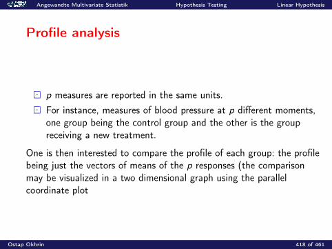
Angewandte Multivariate Statistik Hypothesis Testing Linear Hypothesis
Profile analysis
p measures are reported in the same units. For instance, measures of blood pressure at p different moments,
one group being the control group and the other is the groupreceiving a new treatment.
One is then interested to compare the profile of each group: the profilebeing just the vectors of means of the p responses (the comparisonmay be visualized in a two dimensional graph using the parallelcoordinate plot
Ostap Okhrin 418 of 461
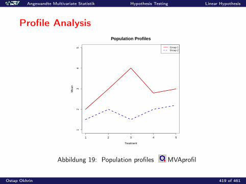
Angewandte Multivariate Statistik Hypothesis Testing Linear Hypothesis
Profile Analysis
1 2 3 4 5
12
34
5
Population Profiles
Treatment
Mea
n
Group 1Group 2
Abbildung 19: Population profiles MVAprofil
Ostap Okhrin 419 of 461
Angewandte Multivariate Statistik Hypothesis Testing Linear Hypothesis
The following questions are of interest:1) Are the profiles similar in the sense of being parallel (which means
no interaction between the treatments and the groups)?2) If the profiles are parallel, are they at the same level?3) If the profiles are parallel, is there any treatment effect (are the
profiles horizontal)?The above questions are easily translated in terms of linear constraintson the means and a test statistic is obviously obtained.
Ostap Okhrin 420 of 461
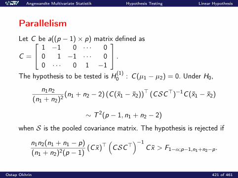
Angewandte Multivariate Statistik Hypothesis Testing Linear Hypothesis
Parallelism
Let C be a((p − 1)× p) matrix defined as
C =
1 −1 0 · · · 00 1 −1 · · · 00 · · · 0 1 −1
.The hypothesis to be tested is H(1)
0 : C (µ1 − µ2) = 0. Under H0,
n1n2
(n1 + n2)2 (n1 + n2 − 2) (C (x1 − x2))> (CSC>)−1C (x1 − x2)
∼ T 2(p − 1, n1 + n2 − 2)
when S is the pooled covariance matrix. The hypothesis is rejected if
n1n2(n1 + n1 − p)
(n1 + n2)2(p − 1)(Cx)>
(CSC>
)−1Cx > F1−α;p−1,n1+n2−p.
Ostap Okhrin 421 of 461

Angewandte Multivariate Statistik Hypothesis Testing Linear Hypothesis
Equality of two levels
The question of equality of the two levels is meaningful only if the twoprofiles are parallel. In the case of interaction (rejection of H(1)
0 ), thetwo populations react differently to the treatments and the question ofthe level has no meaning.The equality of the two levels is written as:
H(2)0 : 1>p (µ1 − µ2) = 0
Ostap Okhrin 422 of 461
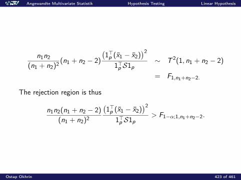
Angewandte Multivariate Statistik Hypothesis Testing Linear Hypothesis
n1n2
(n1 + n2)2 (n1 + n2 − 2)
(1>p (x1 − x2)
)21>p S1p
∼ T 2(1, n1 + n2 − 2)
= F1,n1+n2−2.
The rejection region is thus
n1n2(n1 + n2 − 2)
(n1 + n2)2
(1>p (x1 − x2)
)21>p S1p
> F1−α;1,n1+n2−2.
Ostap Okhrin 423 of 461
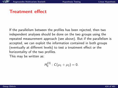
Angewandte Multivariate Statistik Hypothesis Testing Linear Hypothesis
Treatment effect
If the parallelism between the profiles has been rejected, then twoindependent analyses should be done on the two groups using therepeated measurement approach (see above). But if the parallelism isaccepted, we can exploit the information contained in both groups(eventually at different levels) to test a treatment effect or thehorizontality of the two profiles.This may be written as:
H(3)0 : C (µ1 + µ2) = 0.
Ostap Okhrin 424 of 461
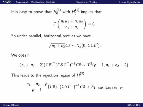
Angewandte Multivariate Statistik Hypothesis Testing Linear Hypothesis
It is easy to prove that H(3)0 with H
(1)0 implies that
C
(n1µ1 + n2µ2
n1 + n2
)= 0.
So under parallel, horizontal profiles we have√n1 + n2Cx ∼ Np(0,CΣC ′).
We obtain
(n1 + n2 − 2)(Cx)>(CSC>)−1Cx ∼ T 2(p − 1, n1 + n2 − 2).
This leads to the rejection region of H(3)0
n1 + n2 − p
p − 1(Cx)>(CSC>)−1Cx > F1−α;p−1,n1+n2−p.
Ostap Okhrin 425 of 461
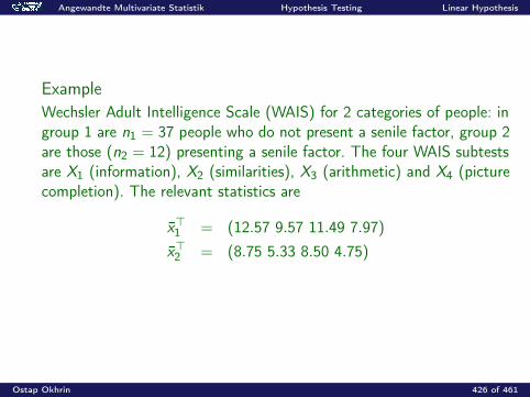
Angewandte Multivariate Statistik Hypothesis Testing Linear Hypothesis
ExampleWechsler Adult Intelligence Scale (WAIS) for 2 categories of people: ingroup 1 are n1 = 37 people who do not present a senile factor, group 2are those (n2 = 12) presenting a senile factor. The four WAIS subtestsare X1 (information), X2 (similarities), X3 (arithmetic) and X4 (picturecompletion). The relevant statistics are
x>1 = (12.57 9.57 11.49 7.97)
x>2 = (8.75 5.33 8.50 4.75)
Ostap Okhrin 426 of 461
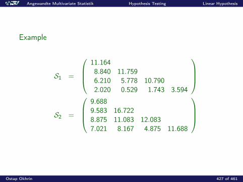
Angewandte Multivariate Statistik Hypothesis Testing Linear Hypothesis
Example
S1 =
11.1648.840 11.7596.210 5.778 10.7902.020 0.529 1.743 3.594
S2 =
9.6889.583 16.7228.875 11.083 12.0837.021 8.167 4.875 11.688
Ostap Okhrin 427 of 461
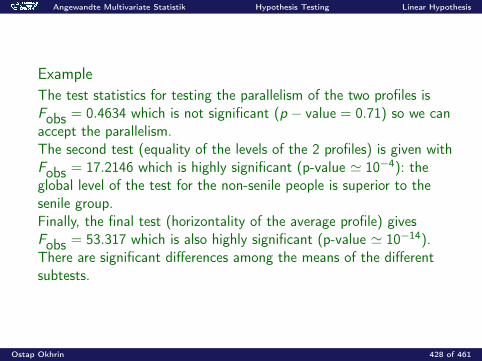
Angewandte Multivariate Statistik Hypothesis Testing Linear Hypothesis
ExampleThe test statistics for testing the parallelism of the two profiles isFobs = 0.4634 which is not significant (p − value = 0.71) so we canaccept the parallelism.The second test (equality of the levels of the 2 profiles) is given withFobs = 17.2146 which is highly significant (p-value ' 10−4): theglobal level of the test for the non-senile people is superior to thesenile group.Finally, the final test (horizontality of the average profile) givesFobs = 53.317 which is also highly significant (p-value ' 10−14).There are significant differences among the means of the differentsubtests.
Ostap Okhrin 428 of 461
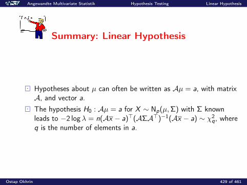
Angewandte Multivariate Statistik Hypothesis Testing Linear Hypothesis
Summary: Linear Hypothesis
Hypotheses about µ can often be written as Aµ = a, with matrixA, and vector a.
The hypothesis H0 : Aµ = a for X ∼ Np(µ,Σ) with Σ knownleads to −2 log λ = n(Ax − a)>(AΣA>)−1(Ax − a) ∼ χ2
q, whereq is the number of elements in a.
Ostap Okhrin 429 of 461
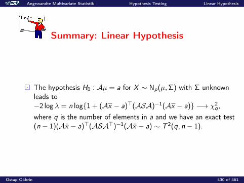
Angewandte Multivariate Statistik Hypothesis Testing Linear Hypothesis
Summary: Linear Hypothesis
The hypothesis H0 : Aµ = a for X ∼ Np(µ,Σ) with Σ unknownleads to−2 log λ = n log1 + (Ax − a)>(ASA)−1(Ax − a) −→ χ2
q,where q is the number of elements in a and we have an exact test(n − 1)(Ax − a)>(ASA>)−1(Ax − a) ∼ T 2(q, n − 1).
Ostap Okhrin 430 of 461
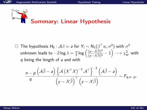
Angewandte Multivariate Statistik Hypothesis Testing Linear Hypothesis
Summary: Linear Hypothesis
The hypothesis H0 : Aβ = a for Yi ∼ N1(β>xi , σ2) with σ2
unknown leads to −2 log λ = n2 log
(||y−X β||2
||y−X β||2− 1)−→ χ2
q, withq being the length of a and with
n − p
q
(Aβ − a
)A(X>X
)−1A>−1 (
Aβ − a)
(y −X β
)> (y −X β
) ∼ Fq,n−p.
Ostap Okhrin 431 of 461
Angewandte Multivariate Statistik Regression Models
Regression Models
Linear Regression
y = Xβ + ε
X (n × p) explanatory variabley(n × 1) response
Ostap Okhrin 432 of 461
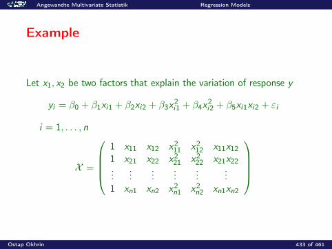
Angewandte Multivariate Statistik Regression Models
Example
Let x1, x2 be two factors that explain the variation of response y
yi = β0 + β1xi1 + β2xi2 + β3x2i1 + β4x
2i2 + β5xi1xi2 + εi
i = 1, . . . , n
X =
1 x11 x12 x2
11 x212 x11x12
1 x21 x22 x221 x2
22 x21x22...
......
......
...1 xn1 xn2 x2
n1 x2n2 xn1xn2
Ostap Okhrin 433 of 461
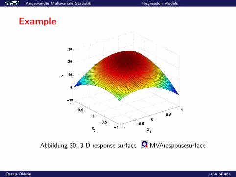
Angewandte Multivariate Statistik Regression Models
Example
Abbildung 20: 3-D response surface MVAresponsesurface
Ostap Okhrin 434 of 461
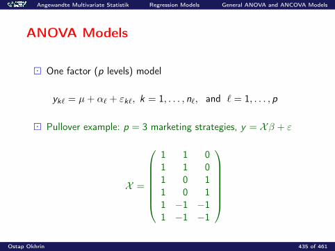
Angewandte Multivariate Statistik Regression Models General ANOVA and ANCOVA Models
ANOVA Models
One factor (p levels) model
yk` = µ+ α` + εk`, k = 1, . . . , n`, and ` = 1, . . . , p
Pullover example: p = 3 marketing strategies, y = Xβ + ε
X =
1 1 01 1 01 0 11 0 11 −1 −11 −1 −1
Ostap Okhrin 435 of 461
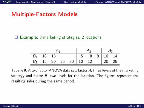
Angewandte Multivariate Statistik Regression Models General ANOVA and ANCOVA Models
Multiple-Factors Models
Example: 3 marketing strategies, 2 locations
A1 A2 A3
B1 18 15 5 8 8 10 14B2 15 20 25 30 10 12 20 25
Tabelle 9: A two factor ANOVA data set, factor A, three levels of the marketingstrategy and factor B, two levels for the location. The figures represent theresulting sales during the same period.
Ostap Okhrin 436 of 461
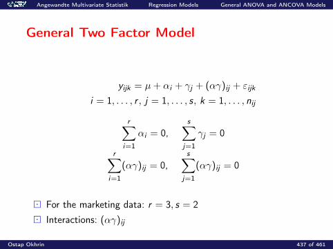
Angewandte Multivariate Statistik Regression Models General ANOVA and ANCOVA Models
General Two Factor Model
yijk = µ+ αi + γj + (αγ)ij + εijk
i = 1, . . . , r , j = 1, . . . , s, k = 1, . . . , nij
r∑i=1
αi = 0,s∑
j=1
γj = 0
r∑i=1
(αγ)ij = 0,s∑
j=1
(αγ)ij = 0
For the marketing data: r = 3, s = 2 Interactions: (αγ)ij
Ostap Okhrin 437 of 461

Angewandte Multivariate Statistik Regression Models General ANOVA and ANCOVA Models
Example
(αγ)11 > 0 The effect of A1 (advertisement in local newspaper)more successful in location B1 (commercial centre)
(αγ)31 < 0 A3 (luxury presentation) less effective in B1 than inB2 (non-commercial centre)
Ostap Okhrin 438 of 461
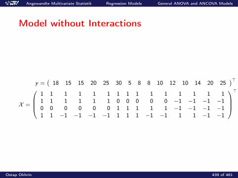
Angewandte Multivariate Statistik Regression Models General ANOVA and ANCOVA Models
Model without Interactions
y =(
18 15 15 20 25 30 5 8 8 10 12 10 14 20 25)>
X =
1 1 1 1 1 1 1 1 1 1 1 1 1 1 11 1 1 1 1 1 0 0 0 0 0 −1 −1 −1 −10 0 0 0 0 0 1 1 1 1 1 −1 −1 −1 −11 1 −1 −1 −1 −1 1 1 1 −1 −1 1 1 −1 −1
>
Ostap Okhrin 439 of 461
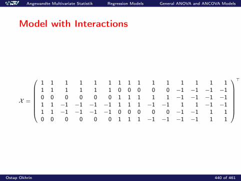
Angewandte Multivariate Statistik Regression Models General ANOVA and ANCOVA Models
Model with Interactions
X =
1 1 1 1 1 1 1 1 1 1 1 1 1 1 11 1 1 1 1 1 0 0 0 0 0 −1 −1 −1 −10 0 0 0 0 0 1 1 1 1 1 −1 −1 −1 −11 1 −1 −1 −1 −1 1 1 1 −1 −1 1 1 −1 −11 1 −1 −1 −1 −1 0 0 0 0 0 −1 −1 1 10 0 0 0 0 0 1 1 1 −1 −1 −1 −1 1 1
>
Ostap Okhrin 440 of 461
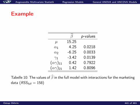
Angewandte Multivariate Statistik Regression Models General ANOVA and ANCOVA Models
Example
β p-valuesµ 15.25α1 4.25 0.0218α2 -6.25 0.0033γ1 -3.42 0.0139
(αγ)11 0.42 0.7922(αγ)21 1.42 0.8096
Tabelle 10: The values of β in the full model with interactions for the marketingdata (RSSfull = 158)
Ostap Okhrin 441 of 461

Angewandte Multivariate Statistik Regression Models General ANOVA and ANCOVA Models
ANCOVA Models
Regression models where some of the variables are qualitative andothers are continuous
Example: Consider the Car data and analyse the effect of weight (W )and displacement (D) on the mileage (M). Test if the origin of the car(C ) has some effect on the response and if the effect of the continuousvariables is same for different factor levels.
Ostap Okhrin 442 of 461
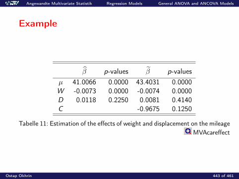
Angewandte Multivariate Statistik Regression Models General ANOVA and ANCOVA Models
Example
β p-values β p-valuesµ 41.0066 0.0000 43.4031 0.0000W -0.0073 0.0000 -0.0074 0.0000D 0.0118 0.2250 0.0081 0.4140C -0.9675 0.1250
Tabelle 11: Estimation of the effects of weight and displacement on the mileageMVAcareffect
Ostap Okhrin 443 of 461
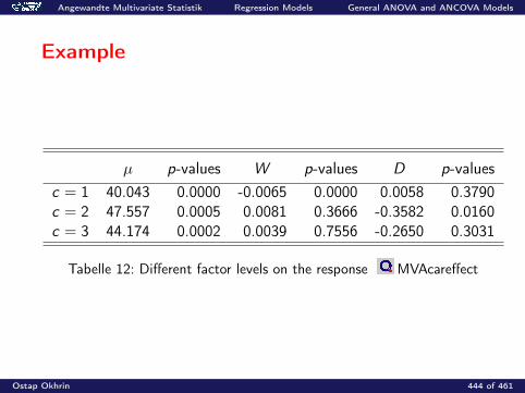
Angewandte Multivariate Statistik Regression Models General ANOVA and ANCOVA Models
Example
µ p-values W p-values D p-valuesc = 1 40.043 0.0000 -0.0065 0.0000 0.0058 0.3790c = 2 47.557 0.0005 0.0081 0.3666 -0.3582 0.0160c = 3 44.174 0.0002 0.0039 0.7556 -0.2650 0.3031
Tabelle 12: Different factor levels on the response MVAcareffect
Ostap Okhrin 444 of 461
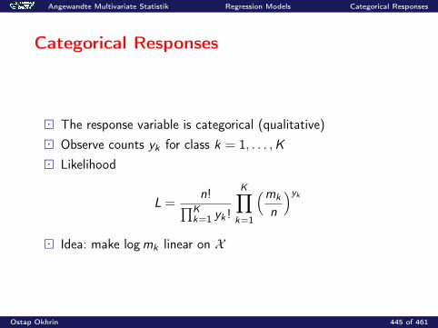
Angewandte Multivariate Statistik Regression Models Categorical Responses
Categorical Responses
The response variable is categorical (qualitative) Observe counts yk for class k = 1, . . . ,K Likelihood
L =n!∏K
k=1 yk !
K∏k=1
(mk
n
)yk Idea: make logmk linear on X
Ostap Okhrin 445 of 461
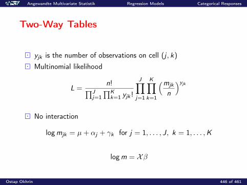
Angewandte Multivariate Statistik Regression Models Categorical Responses
Two-Way Tables
yjk is the number of observations on cell (j , k)
Multinomial likelihood
L =n!∏J
j=1∏K
k=1 yjk !
J∏j=1
K∏k=1
(mjk
n
)yjk No interaction
logmjk = µ+ αj + γk for j = 1, . . . , J, k = 1, . . . ,K
logm = Xβ
Ostap Okhrin 446 of 461
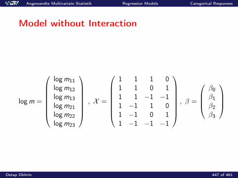
Angewandte Multivariate Statistik Regression Models Categorical Responses
Model without Interaction
logm =
logm11logm12logm13logm21logm22logm23
, X =
1 1 1 01 1 0 11 1 −1 −11 −1 1 01 −1 0 11 −1 −1 −1
, β =
β0β1β2β3
Ostap Okhrin 447 of 461
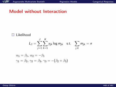
Angewandte Multivariate Statistik Regression Models Categorical Responses
Model without Interaction
Likelihood
Lβ =J∑
j=1
K∑k=1
yjk logmjk s.t.∑j ,k
mjk = n
α1 = β1, α2 = −β1
γ1 = β2, γ2 = β3, γ3 = −(β2 + β3)
Ostap Okhrin 448 of 461
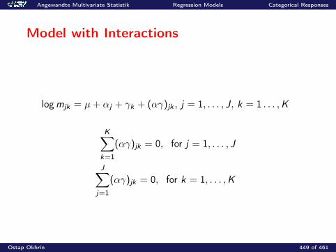
Angewandte Multivariate Statistik Regression Models Categorical Responses
Model with Interactions
logmjk = µ+ αj + γk + (αγ)jk , j = 1, . . . , J, k = 1 . . . ,K
K∑k=1
(αγ)jk = 0, for j = 1, . . . , J
J∑j=1
(αγ)jk = 0, for k = 1, . . . ,K
Ostap Okhrin 449 of 461
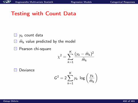
Angewandte Multivariate Statistik Regression Models Categorical Responses
Testing with Count Data
yk count data mk value predicted by the model
Pearson chi-square
χ2 =K∑
k=1
(yk − mk)2
mk
Deviance
G 2 = 2K∑
k=1
yk log(
ykmk
)
Ostap Okhrin 450 of 461
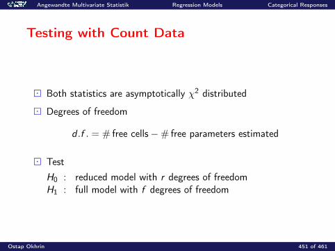
Angewandte Multivariate Statistik Regression Models Categorical Responses
Testing with Count Data
Both statistics are asymptotically χ2 distributed
Degrees of freedom
d .f . = # free cells−# free parameters estimated
TestH0 : reduced model with r degrees of freedomH1 : full model with f degrees of freedom
Ostap Okhrin 451 of 461
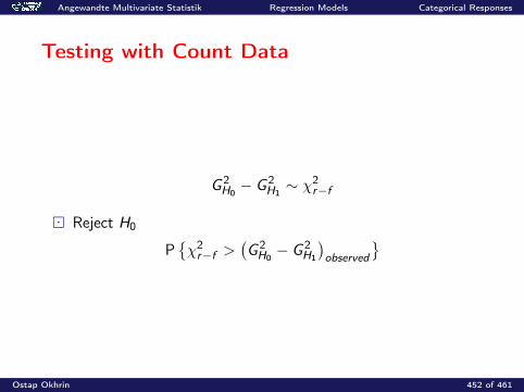
Angewandte Multivariate Statistik Regression Models Categorical Responses
Testing with Count Data
G 2H0− G 2
H1∼ χ2
r−f
Reject H0
Pχ2r−f >
(G 2H0− G 2
H1
)observed
Ostap Okhrin 452 of 461
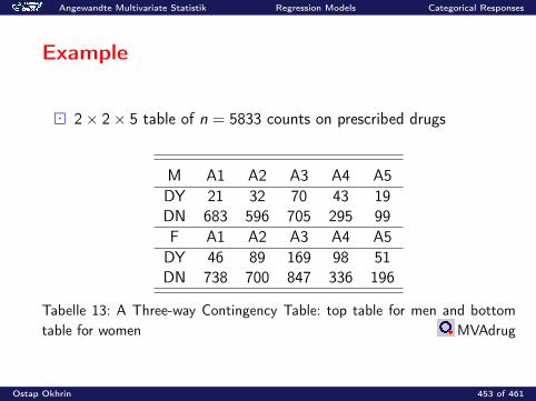
Angewandte Multivariate Statistik Regression Models Categorical Responses
Example
2× 2× 5 table of n = 5833 counts on prescribed drugs
M A1 A2 A3 A4 A5DY 21 32 70 43 19DN 683 596 705 295 99F A1 A2 A3 A4 A5DY 46 89 169 98 51DN 738 700 847 336 196
Tabelle 13: A Three-way Contingency Table: top table for men and bottomtable for women MVAdrug
Ostap Okhrin 453 of 461
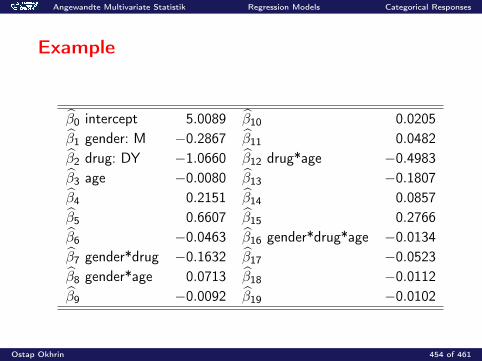
Angewandte Multivariate Statistik Regression Models Categorical Responses
Example
β0 intercept 5.0089 β10 0.0205β1 gender: M −0.2867 β11 0.0482β2 drug: DY −1.0660 β12 drug*age −0.4983β3 age −0.0080 β13 −0.1807β4 0.2151 β14 0.0857β5 0.6607 β15 0.2766β6 −0.0463 β16 gender*drug*age −0.0134β7 gender*drug −0.1632 β17 −0.0523β8 gender*age 0.0713 β18 −0.0112β9 −0.0092 β19 −0.0102
Ostap Okhrin 454 of 461
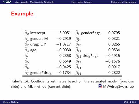
Angewandte Multivariate Statistik Regression Models Categorical Responses
Example
β0 intercept 5.0051 β8 gender*age 0.0795β1 gender: M −0.2919 β9 0.0321β2 drug: DY −1.0717 β10 0.0265β3 age −0.0030 β11 0.0534β4 0.2358 β12 drug*age −0.4915β5 0.6649 β13 −0.1576β6 −0.0425 β14 0.0917β7 gender*drug −0.1734 β15 0.2822
Tabelle 14: Coefficients estimates based on the saturated model (previousslide) and ML method (current slide) MVAdrug3waysTab
Ostap Okhrin 455 of 461
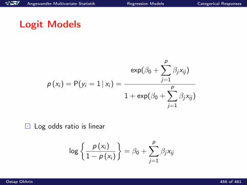
Angewandte Multivariate Statistik Regression Models Categorical Responses
Logit Models
p (xi ) = P(yi = 1 | xi ) =
exp(β0 +
p∑j=1
βjxij)
1 + exp(β0 +
p∑j=1
βjxij)
Log odds ratio is linear
log
p (xi )
1− p (xi )
= β0 +
p∑j=1
βjxij
Ostap Okhrin 456 of 461
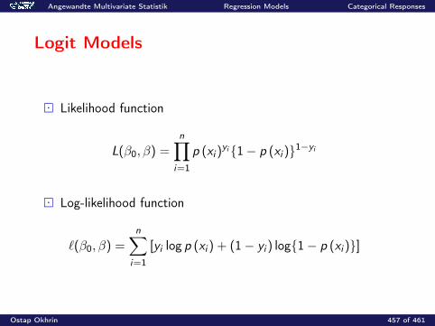
Angewandte Multivariate Statistik Regression Models Categorical Responses
Logit Models
Likelihood function
L(β0, β) =n∏
i=1
p (xi )yi1− p (xi )1−yi
Log-likelihood function
`(β0, β) =n∑
i=1
[yi log p (xi ) + (1− yi ) log1− p (xi )]
Ostap Okhrin 457 of 461
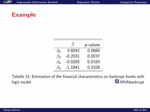
Angewandte Multivariate Statistik Regression Models Categorical Responses
Example
β p-valuesβ0 3.6042 0.0660β3 -0.2031 0.0037β4 -0.0205 0.0183β5 -1.1841 0.3108
Tabelle 15: Estimation of the financial characteristics on bankrupt banks withlogit model MVAbankrupt
Ostap Okhrin 458 of 461
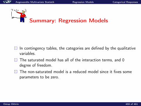
Angewandte Multivariate Statistik Regression Models Categorical Responses
Summary: Regression Models
In contingency tables, the categories are defined by the qualitativevariables.
The saturated model has all of the interaction terms, and 0degree of freedom.
The non-saturated model is a reduced model since it fixes someparameters to be zero.
Ostap Okhrin 459 of 461
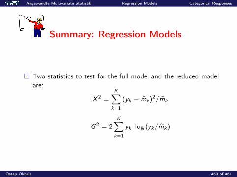
Angewandte Multivariate Statistik Regression Models Categorical Responses
Summary: Regression Models
Two statistics to test for the full model and the reduced modelare:
X 2 =K∑
k=1
(yk − mk)2/mk
G 2 = 2K∑
k=1
yk log (yk/mk)
Ostap Okhrin 460 of 461
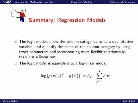
Angewandte Multivariate Statistik Regression Models Categorical Responses
Summary: Regression Models
The logit models allow the column categories to be a quantitativevariable, and quantify the effect of the column category by usingfewer parameters and incorporating more flexible relationshipsthan just a linear one.
The logit model is equivalent to a log-linear model.
log [p (xi )/1− p (xi )] = β0 +
p∑j=1
βjxij
Ostap Okhrin 461 of 461