Inve"tigQción Reo;,ta Mexicana de Física 39, No. 2 (1993) 235-249

A new kind of neural network based on radial basisfunctions

M. SERVÍN AND F.J. CUEVASCentro de Investigaciones en Optica, A. C.Apartado postal 948, León, Gto., México

Recibido el 16 de octubre de 1991; aceptado el 12 de enero de 1993

ABSTRACT.We have derived a new kind of neural network using normalized radial basis functions,"RBF", with the same classifying properties as if it were buUt up using sigmoid functions. Thisequivalence is mathematically demonstrated. In addition, to this, we also show that the proposednetwork is equivalent to a gaussian classifier. The network does not require any computing learningtime to buUd a classifier. This network has been compared with well known adaptive networks,such as backpropagation and linear combination of generalized radial basis functions (GRBF's). Itsadapted forms are presented to see how the classifying regions and boundaries among the suppliedexamples are formed. This neural network can be made to have identical classifying properties, asthe nearest neighborhood classifier "NNC". In the case of having many examples per class, fewercenters can be found using vector quantizing "VQ" techniques as done in Kohonen 's network.Finally, this neural system can also be used to approximate a smooth continuous function, givensparse examples.

RESUMEN. Hemos derivado una nueva clase de redes neuronales usando funciones de base radialnormalizadas, "FBR", con las mismas propiedades de clasificación de una red construida confunciones sigmoides. Esta equivalencia es demostrada matemáticamente. Además, mostramos quela red propuesta es equivalente a un clasificador gaussiano. La red no requiere tiempo de aprendizajepara construir el clasificador. Esta red ha sido comparada con redes adaptivas conocidas, comoel modelo de retro-propagación y una combinación lineal de funciones generalizadas de baseradial. Se presenta CÓmose forman las regiones de clasificación, dado un conjunto de ejemplosde entrenamiento. Esta red neuronal puede ser modelada para tener las mismas propiedades declasificación de un clasificador del vecino más cercano. En el caso de tener varios ejemplos porclase, los centros pueden encontrarse usando técnicas de cuantificación de vectores tal como se usaen la red de Kohonen. Finalmente, este sistema neuronal también puede ser usado para aproximaruna función suave continua, dados puntos dispersos.

PACS: 87.22.J

l. INTRODUCTION

Approximation and c1assification are currently the two most important tasks that neuralnetworks deal with successfully. Since the work of Rumelhart et al. [1] on multilayerfeedforward neural networks and sigmoid based networks of the backpropagation kindhave been the most commonly used neural model for these tasks. Recently Poggio andGirossi [2], emphasized that generalized radial basis functions (GRBF) have many inter-esting properties to be considered seriously as more suitable basis functions lo approx-imate and learn smooth continuous functions from sparse data. The two main learning

236 M. SERVÍN ANO F.J. CUEVAS

procedures mentioned by Poggio and Girossi are: the simple gradient descent on thenetwork's parameter space for oH-line learning (used for backpropagation, too), and theMoore-Peorose pseudoinverse.

However, given a classifying task to be performed, backpropagation classifiers needin general, fewer neurons to classify an input set of feature vectors X in the requiredclasses than a linear combination of GRBF's. Let us take for example, the simplest caseof classifying the entire feature space into two sharply separated regions using aplane,only one high gain sigmoid will be needed to fulfill the aboye requirement. However, thenumber of neurons required using a linear combination of GRBF's to solve the sameclassifying task could be too high. That is one reason why most classifying problems havegenerally been solved using sigmoidal based classifiers.Unfortunately, the backpropagation algorithm for training these sigmoid based net-

works is quite slow. Moreover, in general, there is no way to know in advance the numberof sigmoids the neural system will require to fulfill a given classifying task. The numberof hidden neurons is made large enough to allow for such uncertainties, therefore oftenconstituting a waste of computing power and overfitting.The network described in this work is based on RBF's centered at the data points when

the number of templates per class is not very large. Moreover it is possible to have fewerRBF's than examples using vector quantizing "VQ" techniques [10,11) to distribute theircenters among the data. The approximation and classification of the proposed networkare equivalent to those based on sigmoid functions. In other words, the feature spacecan be filled by back to back hyperpolygons enclosing a unique class forming a Voronoitessellation map [3].The only difference is that, for sigmoid networks, several hyperplanes(neurons) are needed to build up a closed convex region.There is yet another interesting property of the proposed neural network, using smooth

RBF neurons. Making those RBF neurons less selective, a smooth continuous functionwill pass through or near the given set of sparse examples.The learning procedure can be regarded from two points of view. The classical one,

where the examples arrive stochastically in time, so the network learns the given mappingon-line, and the off-line learning, where the complete set of examples and their correctclassification are given at once.

In the earlier years of neural networks [4],on-line learning was an important motivationfor the development of a neural network theory. The on-line learning method is dynamic,that is, the network dynamically wires itself to reduce the error between its current outputand the desired one, often in real time. Due to this, the most widely used method oflearning has been: simple gradient descent. On the other hand, when we have off-linelearning, that is, when it is possible to wait until several examples and their correctclassification has been given, then gradient descent is not generally the best learningprocedure. The reason for this, is the fact of having all the data at once, we implicitlyhave much more information, so it is then possible to use this information surplus to getmuch faster learning algorithms because we can see the future, the present, and the pastsimultaneously. Classical approximation methods can be used to achieve such improvedlearning: the Moore-Penrose pseudoinverse [21, or the conjugate gradient descent. Theproposed network described in this work, is built off-lineoIn the pattern recognition fieldit is very often possible to have several representative templates in advance along with

A NEW KIND OF NEURAL NETWORK.. . 237

their corresponding correct classifications. In this case, classical approximation and wellknown classifying techniques [10] can be used to find the appropriate classifying networkmuch faster than simple gradient descent.

2. THEORETICAL BASIS FOIl THE PROPOSED NEURAL NETWORK

Our starting point to develop a network in which the processors work toward a com-mon goal is statistical mechanics "SM'o. In SM every individual (i.e. atoms, molecules orneurons) will change its state to reduce an energy function called the free energy, F, ofthe system [5], until it reaches its minimum. This state can change stochastically [6] asnormally occurs in nature, or using a deterministic dynamic system to find local minimaclose enough to the global one to be considered as acceptable solutions to the problem athand.

Because of the simple form of the internal encrgy proposed for the classifying task,the minimum of the proposed free energy can be found in just one iteration, that is, nodynamical system is required to find it.

The free energy F of a thermodynamic system at constant temperature can be expressedas [51

F=E-TS, (1)

where E, the internal energy, translates into mathcmatical terms the kind of task weare dealing with. In pattern recognition, the Euclidean distance in the feature space canbe used as a measure of similarity between the incoming data to be classified and thetemplates used to train the network. The parameter T is the absolute temperature andit gives us an indication of how well the task represented by E can be achieved. The lastterm is called the entropy S of the system.

Let us suppose we choose M real valued n-dimensional vectors Ai = (ali, a2i,'" ,an;)as being our set of templates. Thesc templates are chosen to be a complete and represen-tative set of examples in order to guarantee (likc any other pattern recognition system)a reasonably good performance of the system. Additionally, we associated M real valuedclasses Y = (YI, Y2,'" ,Ym), with each of the M templates. \Ve assume we are given, orwe can calculate an estimate of the spread-out of a given class around its templa te. Thisclass-region spread will be expressed as E = (0'1,0'2, .•. , O'AI).

Using the aboye defined terms we can write a free energy for the classifying system as

Al Al""" (X - Af(X - A) """F(X) = L.,¿ • O' I P(X E Ai) + T L.,¿ P(X E Ai) logP(X E Ai),i=l t i=l

providing that

M

¿:P(X E Ai) = 1,i=l

(2)

(3)

238 M. SERVÍN AND F.J. CUEVAS

where P(X E Ai) is the probability that gives us a measure to decide whether an observedfeature vector X belongs to the region surrounding the template Ai.In fact, the term in the internal energy expression which multiplies P(X E Ai), can have

many other mathematical forms with the only condition of being a monotonic increasingfunction of the distance to the template. Changing this isotropic function the networkwill be based on different RBFs. Furthermore, we can even find a representation basedon non-RBFs by using an anisotropic monotonic increasing function. In consequence, thenetwork can be based on a variety of functions. The one presented here is only one typeamong an infinite number of different possibilities.The class to which the observed feature vector X will be assigned, is given by the

fol!owing mathematical expected value:

M

y(X) =L YiP(X E A;).i=1

(4)

Now we have to find the expression for P(X E Ai), which minimizes Eq. (2) subjectto the normalizing, condition given by Eq. (3). Doing this we obtain

(5)

Final!y, Eqs. (4) and (5) constitutes our classifying system.Having chosen (or estimated from the examples) the relative region's hypervolumes

(1;'S, a low value for the T parameter will force the network to behave similarly to amultilayer high gain sigmoid based neural network, so sharp classifying boundaries areformed with the region's hypervolumes, which are proportional to (1i. On the other hand,a high value of this parameter T will make the network behave as formed by a linearcombination of broad Gaussians centered at the examples, so a smooth approximationcurve is then obtained. The topology of the network is shown in Fig. 1.Ifthe network is used as a classifier, then the user should set the temperature parameter

T to the lowest possible value to get the sharpest boundaries among the classes.The ambiguity in choosing the temperature para meter T arises when dealing with

smooth approximation, because for an infinite T, the approximating function becomes aconstant real value equal to the average value of the sparse examples (infinite smoothness).So an additional criterio n should be supplied to find the "best" value for T to set theamount of desired smoothness. Due to the wide range of applications this approximationcan be used for, no particular criterion has been given and the user should find the mostappropriate one to find the "best" T depending upon its particular application.Making al! the (1;'S equal, and using a very low value for the T parameter, the classifying

properties of the network become those of a NNC because it divides the feature spaceexactly in the same way as a NNC, so any figure of merit, limitation or applicationreported concerning the NNC, will directly be applied to this network. AIso the featurespace segmentation will be that of a Voronoi tessel!atioll mal'.

A NEWKINDOFNEURALNETWORK.. . 239

y(x I •••••X,) =• -El, -, ¡i.¿ Ji e l" J IJ ,~.~ -Él, -, ji.1_1 e'.' J IJ ,

FIGUREl. Topologyoí the praposed neura!network.E""h circlein the first hidden laye, representsneuraos having gaussian kind oí response centered at the training examples.

In the case of clustered, noisy data, we can reduce network size by finding the mean anddeviation for clusters formed by the featme vectors and assign one neuran per cluster. Fora given class there may be several clusters that can be sufliciently close to be consideredas connected and these connections can make up class regions with complicated forms.Having this in mind, we can rewrite Eq. (5) as function of these local averages andvariances as

Y(X) = L:~~YIexp h+'(X - EA,f(X - EA,)],¿'=I exp [-rk(X - EA,)T(X - EA,)]

where EA, and (1; are given as

(6)

(7)

(8)

where Ak represents the templates belonging to cluster i. IN;I is the number of examplesof cluster i, which belong to class Vi. As shown from Eqs. (7) and (8), EA, is the centerof mass for cluster i and (1i gives us a measure of how spread those examples are from itscenter of mass.Another alternative (which works much better) to ¡¡nd less Gaussian centers than ex-

amples, is obtained by using vector quantizing (VQ) techniques. This technique has beenused by Kohonen [9Jin a self-organizing neural network. The application and consequencesof this techniques coupled with the nemal model herein described is now developing andwill be published in a future papero

240 M. SERVÍNAND F.J. CUEVAS

3. A COMMENT ON TIIE SMOOTH FUNCTION APPROXIMATION PROBLEM

So far we have concentrated on the classifying problem, now we briefly mention (withoutany formal proof whatsoever) how the proposed network can be used to approximate asmooth function which passes through or near the data points.The easiest way of approximating a smooth function from examples (Ai, Yi) using the

proposed network, is, as mentioned before, by making the T parameter relatively large.This simple procedure gives reasonable approximations as shown in the experimentalresult sections. Another way to proceed is to add another term to the internal energyexpression which encodes this smoothness condition. This additional term is called aregularization term [21. This procedure gives, in general, far better smooth approximation.\Ve do not follow this approach but it is worth mentioning because it is the root of a moregeneral way of approximating smooth functions to sparse data [21.

4. EQUIVALENCE BETWEEN NORMALIZEO RBF NETWORKS ANO SIGMOID BASEO ONES

\Ve show in this section how, for a two class problem, the regio n boundary is formedbetween the two classes using Eqs. (4) and (5), and the condition needed to reduce it toa network based on sigmoid function with linear argument.If we have two n-dimensional real valued template vectors A = (al, a2, ... , an) and

E = (bl, b2, ... , bn), which belong lO lhe real valued classes YI and Y2 respectively, theproposed neural network has lhe following input-outpUl relationship:

y(X) = YI exp[-gl(X - A)T(X - A)I + Y2 exp[-g2(X - Ef(X - E)] (9)exp[-gl(X - A)T(X - E)) + exp[-g2(X - A)T(X - E) ,

where we have made gi = l/(Ta;) for i = {l,2}. \Vhen both gains 91 and 92 are equal,the proposed network can algebraically be lransformed into

y(X) - YI + Y2 - Yl- 1+ exp [-2g1(E - A)T (X - AtB)]' (10)

which is a sigmoid function with linear argument. The boundary between the classes is anhyperplane halfway and perpendicular to the !ine connecting both templates. For example,in a two dimensional feature space (X,Y), if we have two templates at A = (a\,a2) anoE = (b¡, b2), according to Eq. (10) the bOllndary will lie on the following straight !ine:

Yal - bl b; - a; + b~ - a~

= --X + ------b2 - a2 2(b2 - a2)

\Vhen the gains gl and 92 are different Eq. (10) becomes

(11)

y(X) = Yl + Y2 - Yl (12)1+ exp[(g2 - 9¡ )XTX - 2(92E - 91A)TX + g2ETE - gl AT Al'

A NEW KIND OF NEURAL NETWORK. .. 241

The argument of the sigmoid function looks like a complicated quadratic hypersurfacebut it is in fact a hypersphere. To show it in a simple way let us suppose that the twofeature vectors are: A = (0,0, ... ,O) and B = (b, O, ... ,O), that is, A is situated at theorigin and B at a distance b from A. Furthermore let us consider (92/91) = 1/ as the spreadratio between the two elasses. Using those values in the sigmoid argument of Eq. (12),the boundary wil! lie within the set of points X which satisfy

( b) T ( b) b2X - _1/_1 X - _1/_1 - 1/ = O,1/-1 1/-1 (1/-1)2 '

1=(1,1,... ,1). (13)

As can be analyzed from Eq. (13), if the spreading ratio is set to 1/ > 1 then the hyper-sphere wil! enelose the B example. Otherwise with 1/ < 1 the hypersphere wil! enelosethe A template. If 1/ = 1, then the infinite radius hypersphere becomes the separatinghyperplane discussed aboye. Additionally, if 1/ » 1 then the hypersphere surrounding theB example collapses at the template's point B. That means, having the extreme case of1/ = 00 the only feature vectors assigned to the Y2 regio n will be those exactly equal toB. On the other hand if 1/ « 1, the hypersphere collapses in example A.If this problem is solved in two dimensions using sigmoid network with backpropagation,

we would need at least three sigmoid neurons to build a elosed region. Furthermore, ifthe number of dimensions of the feature space grows, the number of hyperplanes neededto build a convex elosed regio n wil! grow proportionally. Consequently, the number ofbackpropagation neurons depends also on the dimensions of the feature space for a similarelassifying task.From this discussion it can be seen that the proposed model is in fact a generalization

of the commonly used sigmoid when the linear term in its argument is replaced by aquadratic function, and by using isotropic Gaussians the boundaries formed between theelasses are hyperspheres. Using another RBFs or non-RBFs the model can give rise toother boundary functions (elosed or open) such as ellipses, parabolas, etc., with probableadditional interesting properties not yet explored.\Ve conelude this section by recalling that if all the ai 's are set to an equal value

and T --> 0, then the network proposed can be switched into a network based on highgain linear argument sigmoid functions. Its properties, merits and limitations are thesame as for a NNC. Otherwise, if the a;'s are different, the network is stil! switcheableinto a sigmoid based network but now the boundaries among the elasses are portions ofhyperspheres and its elassifying properties are like as for a MLC system. This wil! bediscussed in the next section.

5. RELATION OF THE PURPOSED MODEL TO GAUSSIAN CLASSIFIERS

In this section, it is shown that the neural network proposed is mathematically equivalentto a Gaussian maximum likelihood elassifier "GMLC" [8). Moreover, introducing addi.tional prior knowledge (the prior probability of the templates) the presented network canbe transformed into a Gaussian estimator.

242 M. SERVÍN AND F.J. CUEVAS

Let US suppose we have M templates Ai in an n-dimensional feature space. Each timewe sample the outside world (which is our source of vectors X) a feature vector X isgenerated. Having this input vector X, we have to look at the stored templates Ai, andchoose the template which resembles the mosto This selection is done according to sorneprior knowledge of how these X are generated. Once we have chosen the most similartemplate Ai, then we can associate to the X the class Yi to which the template Aibelongs.

One way of specifying the mechanism used by the source to generate those X, is es-timating or assuming prior probabilities. The conditional prior probability, p(X I .4i).gives us a measure in the sense that: having observed a feature vector X, a noisy processfrom Ai was generated. The other one is the prior probability p(Ai), which gives us ameasure of the relative frequency of sampling a noisy version of Ai among the other M - 1possibilities.

Those two probabilities are commonly used to find the posterior probability, which givesus a similarity measure to choose Ai given X. Using the Bayes' formula, this probabilityreads as

(A I X) = p(Ai)p(X I Ai)P 1M' 2::j=1 p(Aj)p(X I Aj)

(1 .;; i .;;M), (14)

and its class will be given by the following expected value:

M

y(X) = LYiP(Ai IX).i;:::1

(15)

Many probability distributions are represented by smooth continuous functions, in conse-quence Eq. (14) gives us continuous real numbers in the range (0,1). To choose the mostprobable one, we have to select the p(Ai I X) with the highest value. Once this selectionhas been done, the remaining probabilities are set to 0, and the selected one to 1. In thisway Eq. (15) will give us only a possible class, and not a weighted average of them.

If the distribution of the feature vectors X are Gaussians (or assumed to be Gaussians)with variance equal <7i and centered at the templates Ai, and having the same chance ofsampling any Ai, then, the resulting classifier given by Eqs. (14)-(15) looks similar to theproposed network, with the exception that the temperature parameter T is set to one.AIso the network as stated by Eq. (14) and Eq. (15) is the same as the one reported byMoody and Darken [91, which performs a soft competition among the classes. In otherwords, it approximates a smooth surface, so no sharp classifying is obtained (the "winnertakes all" process is not achieved).

Adding the temperature parameter T to Eq. (14) as done in the proposed model, thenthe maximum selection process is achieved simultaneously to the process of computingp(Ai I X). In' this way a GMLC is obtained.

Moreover as mentioned before, the proposed network will perform in parallel a Gaussianmaximum likelihood classification of the input vector X. To show it, in a simple way, let's

A NEWKINDOF NEURALNETWORK.. . 243

•• ••

FIGURE2. Sel of represenlalive lemplales used lo build lhe classifying neural nelwork. The graylevel of lhe small circles represenls one of four differenl classes of lhe problem. The dol in lheircenler is lhe exacl lemplales coordinales in lhe fealure space.

return to our simple two class problem of Section 4. For this classifying task, we can writethe likelihood ratio as

where the decision is taken according lo [81.1. Assign A if ¡(X) > 1,2. Assign B if ¡(X) < 1,3. Make an arbitrary decision at the boundary: ¡(X) = 1.The decision boundary (statement 3 aboye) is the same hypersphere as the boundary

formed by the proposed network. This section has shown that, if the probability of se-lecting an Ai is not evenly distributed, the Bayesian Gaussian classifier gives a betterperformance. Olherwise lhe Gaussian-Bayesian classifier is reduced lo a GMLC with lhesame properties as the proposed neural system.

6. EXPERI~IENTAL RESULTS

The proposed network has been tested to show its classifying, interpolation and ap-proximation capabililies. Fig. 2 shows a two dimensional feature region at which the12 examples used to build the proposed nelwork are shown. The gray level of the circles,which surround each template represents one possible class. The example coordinates andlheir corresponding classes were generated at random inside the region.After feeding the templales' coordinales and lheir corresponding classes, iuto lhe pro-

posed nelwork [Eqs. (4) and (5)1, the nelwork creales the classifying topography shownat Fig. 3. The parameter T has been set lo a small value and lhe {}"i'S have been chosen all

244 M. SERVÍNANDF.J. CUEVAS

FIGURE3. Sharp region boundaries formed by the proposed neural network given lhe classifyingtask shown at Fig. 2. The variance from the templates have been set equal to 1. The temperatureparameter T has been set to a low value to obtain sharp classifying boundaries.

equal to one. Fig. 3 shows how sharp boundaries between the classes are formed and thoseboundaries fal! half way hetween the examples. This classifier has the same behavior as theNNC, but with substantial!y faster computing capabilities when a ful!y paral!el hardwareor a vector based digital machine is used. Fig. 4 shows the same classifying problem butnow the 0';'5 of the white regions have been increased so its classifying area has grownand the region boundaries are now arc segments belonging to the boundaries circles.Fig. 5 shows the same examples and classes shown in Fig. 2, but there the parameter T

has been increased. Their deviations from their templates have been taken equal to one.It can now be seen that a smooth curve passing through or near the examples has beenformed. This is almost the kind of smooth functions that would be obtained if we hadtrained a RBF's kind of network centered at these examples.

i. COMPARISON TO SIGMOIDAND GAUSSIANADAPTIVE CLASSIFIERS

The most traditional approaches in adaptive neural networks have also been tesled usingthe same classifying problem for comparison purposes. \Ve have used the fol!owing ap-proximations for the sigmoidal or backpropagation neural network and for the Gaussianone:

~ ['¿""(X-cY]jj(x¡, X2) = ~ h; exp - f;;; ] O' .] , (lia)

A NEWKINDOF NEURALNETWORK.. . 245

FIGURE4. Same dassifying task shown in Fig. 2, bul in this case lhe varialions for the lemplatesassigned to the brighter dass has been doubled, so its region dass has grown.

FIGURE5. Same dassifying lask as shown in Fig. 2, but in this case lhe "lemperature" parameterT has been raised, to change lhe behavior of the network fram a sharp dassifier to a smoolhapproximator.

ydx¡, X2) = (Jk (t hik(Ji (t XjWijk - Cjk)) k E (0,1), (17b)1=1 )=1

(18)

246 M. SERVíNANDF.J. CUEVAS

FIGURE6. Classifying topography created by the network based on Gaussian functions when thetemplates and classes in Fig. 2 where supplied to the adaptive network. It can be seen how sornewell classified templates are in the raising edge of a basis function making even very close observedfeature vectors be missclassified.

and the error has been defined as:

12E = 2:Jy(alk>a2k) - Yk)2,

k=1

(19)

as in the proposed network the classes' numeric values were chosen to be 0,1,2 and 3.The number of neurons used for the GRBF network was 50, and 15 for the sigmoid basedone. The equations of motion for the adaptive systems were the simple gradient descentover the error surface E, in the network's parameter space, that is

8Ehi = -'18hi'

8ECij = -11--,8c,j

(20)

for the GRBF network and for the sigmoid network

8EWijk = '1-8--,Wijk

(21 )

where '1 is the rate of convergence or gain for the detenninistic adaptive neural systems.The aboye adaptive networks were tested solving the classifying task shown at Fig. 2.

These networks have created the regions and boundaries shown at Figs. 6 and 7 for theGaussian and the sigmoid networks respectively. The error over the 12 examples given byEq. (18) has been almost zero after the adaptive process.

A NEWKINn OF NEURALNETWORK.. . 247

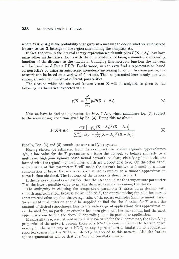
FIGURE 7. Classifying topography created by the backpropagation kind of neural network whenthe templates and classes shown at Fig. 2 were supplied to the adaptive network. It can be seenhow the classification topography has completely changed with ,eference to the Gaussian basednetwo,k and the proposed one. The same problem that sorne templates are on the raising edge ofthe basis functions is also presented in this case.

From these Figures mainly two things can be observed: firstly the created regions aresometimes not sharply classified, especially in the Gaussian case, unless many Gaussianneurons were used; secondly, quite often the class regions are not plateau having the samegray leve!. Frequently sorne well classified examples may fall on the raising edge of a basisfunction making even very close input feature vectors to be missclassified, as can be seenfrom Figs. 6 and 7. What is normally done in such systems to improve the regions plateauis to provide the neural system with many examples per class around its average to spreadout the class' region.Finally, before leaving this section it is worthwhile showing the class regions created

by the NNC using the same classifying task, so we can compare it with the topographycreated by the proposed network when all (Jis are equa!. These class regions are shownin Fig. 8. lt can be observed how the class boundaries are formed in the same way asthe proposed network with the exception that, the nearest neighborhood classifier has thesharpest boundaries among the classes, given that it is not a continuous function as theproposed one.

8. CONCLUSIONS

A new kind of network for classification and approximation based on RBFs has beenobtained. Their capabilities and the condition needed to switch it into a linear argument,sigmoid based network has been considered. Comparison of well known approaches such

248 M. SERVÍNANDF.J. CUEVAS

FIGURE8. Classifying topography erealed by lhe nearest neighborhood classifier for the classifyingtask shown in Fig. 2. It can be observed how the separating boundaries between the examples areexaetly the same as the ones erealed by the proposed neural nelwork shown in Fig. 3. The soledifferenee is lhat lhese boundaries are even sharper, given lhat lhe nearesl neighborhood classifieris not a continuous function in the feature space.

as baekpropagation, GRBF's, NNC, Bayesian classifier and MLC, have also been poinledout.The main advantage of this approaeh is lhal having lhe examples and its eorreel clas-

sifiealion in advanee, they can be fed inlo lhe network just as lhey are, and no gradienldeseent training or matrix inversion are needed lo build up the right classifying network,that is, the network requires no learning. Ir we have many noisy examples, slalisliealreduetion can be used lo find fewer eenters and their associated deviations per class.These two numbers are fed into the redueed network. Moreover it has been shown how wecan eontinuously ehange the behavior of the network from a sharp classifier lo a smoolhfunetion approximator by ehanging jusI one parameter, whieh is the value of lhe absolutelemperature T of the system.This network can also learn on-line under gradient deseent. Its behavior, eapabilities

and learning rates are now being researehed.

ACKNOWLEDGEMENTS

\Ve wish to aeknowledge Dr. J.L. Marroquin's useful suggestions throughout the devel-opment of this work. \Ve also with to aeknowledge Pro£. Stephen Grossberg's fruitfuleomments to improve the presentation of this work.

A NEW KIND OF NEURAL NETWORK. . . 249

REFERENCES

1. D.E. Rumelhart, G.E. Hinton, and R.J. Williams, "Learning internal representations byerror propagation" I in ParaIlel di3tributed processing: explorations in the microstructures o/cognition 1, D.E. Rumelhart and J.L. McClelland (eds.) Cambridge, MA, MIT Press (1986)318.

2. T. Poggio and F. Girossi, "A theory 01 networks for approximation and learning", in MITA.I. Memo 1140 (1989), C.B.I.P. paper No. 31.

3. J.O. Murphy, "Nearest neighbor pattern classification perceptrons", in Proceedings o/ theIEEE 78 (1990) 1595.

4. R. Rosenblatt, Principies o/ neurodynamics, New York, Spartan Books (1959).5. G.E. Hinton, Neural Computing 1 (1989) 143.6. S. Kirpatrick, C.D. Gelatt Jr. and M.R. Vecchi, Science 220 (1983) 671.7. J.J. Hopfield, "Neural networks and physical systems with emergent collective eomputational

abilities", in Proceedings o/ the National Academy o/ Seienee USA 79 (1982) 2554.8. J.T. Tou, R.C. Gonzalez, Pattem recognition principies, Massaehusetts, Addison-Wesley

Publishing Company (1974).9. J. Hertz, Krogh A., Palmer, R.G. Introduction to the theory o/neural computation, California,

Addison-\Vesley Publishing Company (1991).10. J. Makhoul, S. Roncos and H. Gish, ¡¡Vector quantization in speech codingll, in Proceedings

o/ the IEEE 73, 11 (Nov. 1985) 1551.11. R. Duda, P. Hart, Pattem classification and scene analysis, Wiley-Interscience Publication

(1973).