An efficient numerical approach tomodel wave overtopping of rubblemound breakwaters

M.L.A. Moretto

TechnischeUniversiteitDelft

Photo cover image:X-bloc breakwater with wave wall along the coastline of Panama City.Source: Personal image,September 2019Copyright ©

The presented work was conducted and carried out in cooperation withRoyal HaskoningDHV.

Copyright ©All rights reserved.

An efficient numerical approach to model waveovertopping of rubble mound breakwaters

by

M.L.A. Moretto

For the degree of Master of Science in Civil Engineering at Delft Universityof Technology

February 17, 2020

An electronic version of this thesis is available at http://repository.tudelft.nl/.

DELFT UNIVERSITY OF TECHNOLOGYDEPARTMENT OF

HYDRAULIC ENGINEERING

The undersigned hereby certify that they have read and recommend to the Faculty of CivilEngineering and Geosciences (CEG) for acceptance a thesis entitled

An efficient numerical approach to model wave overtopping of rubble mound breakwaters

by

M.L.A. Moretto

in partial fulfillment of the requirements for the degree of

MASTER OF SCIENCE CIVIL ENGINEERING AND GEOSCIENCES (CEG)HYDRAULIC ENGINEERING

at the Delft University of Technology

Dated: February 17, 2020

Thesis committee:

Chairman:Dr. ir. Antonini, A.Delft University of TechnologyHydraulic EngineeringCoastal Engineering

Members:Ir. van den Bos, J.Delft University of TechnologyHydraulic EngineeringCoastal Engineering

Dr. Tissier, M.F.S.Delft University of TechnologyHydraulic EngineeringEnvironmental Fluid Dynamics

Ir. van der Lem, C.Royal HaskoningDHVMaritimeSenior Port Engineer

Ir. drs. Boersen, S.Royal HaskoningDHVRivers & CoastsHydraulic & Coastal Engineer

Preface

This research marks the last stage of the master in Civil Engineering at the Delft University of Technol-ogy, Faculty of Civil Engineering and Geosciences. It has been the last challenge in obtaining the titleof Master of Science in the field of Hydraulic Engineering.

This thesis was carried out in collaboration with the Rivers & Coasts Department at Royal Haskon-ingDHV, which makes considerable efforts to create innovative design tools for coastal defences. Inline with this ambition, Royal HaskoningDHV joined Boskalis Westminster, van Oord and Deltares in aJoin Industry Project (JIP) named ”JIP CoastalFOAM”, which aims to contribute to the validation andexpansion of a numerical model as design tool. I would like to thank Royal HaskoningDHV for theprovided opportunity, resources and internal knowledge to perform this thesis at their offices in Rot-terdam. I take this opportunity to express my gratitude to all the persons who had an impact on thisfinal work.

My special thanks go to Alessandro Antonini for his constant and valuable guidance. His knowledgeabout the OpenFOAM package and numerical modelling was essential and highly appreciated. Hisinput at every meeting and availability for discussion have substantially increased the quality of thisresearch. Jeroen van den Bos’ input, guidance and knowledge on rubble mound breakwaters and nu-merical modelling have helped me throughout the process. Always present at every progress meetingand willing to take the time to spar and discuss, which was greatly appreciated. I would like to thankMarion Tissier as well, for her precious feedback and time. Her contribution has certainly helped inincreasing the quality of this report.

I would also like to express my deep gratitude to both my supervisors at Royal HaskoningDHV, Cockvan der Lem and Stef Boersen. They have welcomed, introduced and guided me all along the way,offering me also the opportunity to attend my first scientific conference in Panama City, the 38 IAHRworld congress with as theme ”Water - Connecting the World”. Their continuing assistance and feed-back were essential.

Lastly, I would like to thank my family and friends for their personal support during these months.Without their encouragement it would not have been an enjoyable and instructive journey.

M.L.A. MorettoDelft, February 17, 2020

iii

Abstract

Worldwide, rubble mound breakwaters are designed and built to shelter and protect coastal areas fromovertopping and flooding, especially harbours and shorelines. Rubble mound breakwaters are essentialto preserve desired hydraulic conditions within the hinterland, avoiding damage to inhabited or indus-trial areas. This research focuses on the wave overtopping of rubble mound breakwaters as failuremechanism. To assess the wave overtopping engineers can adopt multiple methods. These methodscan be ordered in increasing degree of accuracy and costs: empirical methods, neural networks, nu-merical models and physical laboratory experiments. The preliminary design phase is a highly iterativeprocess. Using physical laboratory experiments within this phase is an expensive choice, therefore em-pirical methods are often preferred. Nevertheless, this research revealed that empirical methods, e.g.the so called EurOtop 2018, show significant shortcomings in assessing average overtopping quantitiesover rubble mound breakwaters, even more when the geometrical complexity of the structure increases(presence of protruding wave wall). This thesis re-calibrated the roughness coefficient proposed bythe original EurOtop 2018 approach, referred to as the updated EurOtop 2018 method.

Numerical models are proposed as a possible solution between empirical methods (which can be car-ried out quickly given their low complexity) and physical laboratory experiments (which need moretime but are characterised by high accuracy). They have been increasingly used and accepted in thepast decades. Following this trend, the Joint Industry Project (JIP) CoastalFOAM 1 was launched withthe objective to develop and validate a numerical model (OpenFOAM, waves2Foam, OceanWaves3Dand JIP additions; referred to as CoastalFOAM) capable of accurately modelling the wave-structureinteraction of rubble mound breakwaters. This research aims to calibrate and evaluate the Coastal-FOAM model to assess small to large wave overtopping of rubble mound breakwaters with protrudingor non-protruding wave wall, considering 500 waves. The evaluation of CoastalFOAM shows that thisnumerical model can be used, instead of empirical methods (e.g. updated EurOtop 2018), to assessthe average overtopping discharges. CoastalFOAM showed excellent agreement with measurementsfor large and medium overtopping cases, while resulting less accurate for small overtopping cases.

The analysis revealed, however, that the average overtopping discharge as a quantity is not capa-ble of identifying the magnitude of large overtopping events (without modelling all 500 waves). Thiscan be considered critical in determining whether the structure is safe enough in terms of ServiceabilityLimit State (SLS) or Ultimate Limit State (ULS). Consequently, this thesis proposes a new methodologyto assess the maximum overtopping volume within a storm, applying the concept of wave focusingand using the NewWave theory. The input variables for the NewWave profile are extracted from thespectral properties at the toe of the breakwater. A first order wave maker is used to generate theNewWave profile, making the methodology sensitive for the degree of non-linearity of the consideredwave conditions. This NewWave methodology offers improved accuracy to assess the maximum over-topping volumes when compared to the EurOtop 2018 approach. Furthermore, this research proposesto apply the inverse EurOtop 2018 technique to assess the average overtopping discharge using theNewWave maximum overtopping volume. However, the accuracy of this methodology is lower thanthat obtained with the updated EurOtop 2018 guidelines.

This study shows that CoastalFOAM can be used, instead of the current empirical methods, to assessthe average overtopping discharge within the design cycle of rubble mound breakwaters. However,according to what has emerged, CoastalFOAM shows to be less accurate in calculating small overtop-ping discharges as opposed to medium and large. On the other hand, when considering the maximumovertopping volume as design criterion the proposed NewWave methodology showed to be the mostefficient and accurate.

1The Joint Industry Project (JIP) CoastalFOAM was founded in 2015 by the following engineering companies: Royal Haskon-ingDHV, Boskalis Westminster, van Oord and Deltares.

v

Contents

Preface iii

Abstract v

List of Figures ix

List of Tables xv

1 Introduction 11.1 Importance of this research. . . . . . . . . . . . . . . . . . . . . . . . . . . . . . . . . 11.2 Coastal structures . . . . . . . . . . . . . . . . . . . . . . . . . . . . . . . . . . . . . . 21.3 Numerical models . . . . . . . . . . . . . . . . . . . . . . . . . . . . . . . . . . . . . . 31.4 Problem definition and description . . . . . . . . . . . . . . . . . . . . . . . . . . . . 31.5 Research objective and questions . . . . . . . . . . . . . . . . . . . . . . . . . . . . . 41.6 Research methodology. . . . . . . . . . . . . . . . . . . . . . . . . . . . . . . . . . . . 4

2 Physical experiments 72.1 Introduction . . . . . . . . . . . . . . . . . . . . . . . . . . . . . . . . . . . . . . . . . . 72.2 Geometry . . . . . . . . . . . . . . . . . . . . . . . . . . . . . . . . . . . . . . . . . . . 72.3 Wave parameters . . . . . . . . . . . . . . . . . . . . . . . . . . . . . . . . . . . . . . . 82.4 Validation cases . . . . . . . . . . . . . . . . . . . . . . . . . . . . . . . . . . . . . . . 9

3 Empirical Methods 113.1 Introduction . . . . . . . . . . . . . . . . . . . . . . . . . . . . . . . . . . . . . . . . . . 113.2 Average overtopping formulas . . . . . . . . . . . . . . . . . . . . . . . . . . . . . . . 113.3 Comparison . . . . . . . . . . . . . . . . . . . . . . . . . . . . . . . . . . . . . . . . . . 153.4 Provisional conclusions . . . . . . . . . . . . . . . . . . . . . . . . . . . . . . . . . . . 17

4 Numerical Model 194.1 Introduction . . . . . . . . . . . . . . . . . . . . . . . . . . . . . . . . . . . . . . . . . . 194.2 Numerical framework . . . . . . . . . . . . . . . . . . . . . . . . . . . . . . . . . . . . 194.3 Mathematical model . . . . . . . . . . . . . . . . . . . . . . . . . . . . . . . . . . . . . 204.4 Wave generation . . . . . . . . . . . . . . . . . . . . . . . . . . . . . . . . . . . . . . . 234.5 Ventilated boundary . . . . . . . . . . . . . . . . . . . . . . . . . . . . . . . . . . . . . 244.6 Overtopping . . . . . . . . . . . . . . . . . . . . . . . . . . . . . . . . . . . . . . . . . . 244.7 Numerical set-up . . . . . . . . . . . . . . . . . . . . . . . . . . . . . . . . . . . . . . . 25

5 Model validation 275.1 Introduction . . . . . . . . . . . . . . . . . . . . . . . . . . . . . . . . . . . . . . . . . . 275.2 Calibration case and procedure . . . . . . . . . . . . . . . . . . . . . . . . . . . . . . 275.3 Calibration of numerical model . . . . . . . . . . . . . . . . . . . . . . . . . . . . . . 285.4 Evaluation of medium overtopping cases. . . . . . . . . . . . . . . . . . . . . . . . . 355.5 Sensitivity analysis. . . . . . . . . . . . . . . . . . . . . . . . . . . . . . . . . . . . . . 395.6 Evaluation of large overtopping cases. . . . . . . . . . . . . . . . . . . . . . . . . . . 425.7 Evaluation of small overtopping cases . . . . . . . . . . . . . . . . . . . . . . . . . . 445.8 Summary . . . . . . . . . . . . . . . . . . . . . . . . . . . . . . . . . . . . . . . . . . . 46

6 Model application 496.1 Introduction . . . . . . . . . . . . . . . . . . . . . . . . . . . . . . . . . . . . . . . . . . 496.2 Importance of the maximum overtopping volume. . . . . . . . . . . . . . . . . . . . 496.3 Focused wave group . . . . . . . . . . . . . . . . . . . . . . . . . . . . . . . . . . . . . 516.4 The NewWave theory. . . . . . . . . . . . . . . . . . . . . . . . . . . . . . . . . . . . . 516.5 Application of the NewWave theory . . . . . . . . . . . . . . . . . . . . . . . . . . . . 53

vii

viii Contents

6.6 Methodology to assess the maximum overtopping volume (𝑉 ) . . . . . . . . . . . 536.7 Methodology to assess the average overtopping discharge, 𝑞 . . . . . . . . . . . . . 64

7 Comparison with empirical methods 677.1 Introduction . . . . . . . . . . . . . . . . . . . . . . . . . . . . . . . . . . . . . . . . . . 677.2 Comparison EurOtop 2018 with CoastalFOAM, 𝑞 . . . . . . . . . . . . . . . . . . . 677.3 Comparison EurOtop 2018 with NewWave methodologies . . . . . . . . . . . . . . 717.4 Provisional conclusions . . . . . . . . . . . . . . . . . . . . . . . . . . . . . . . . . . . 75

8 Discussion, conclusions and further research 778.1 Discussion. . . . . . . . . . . . . . . . . . . . . . . . . . . . . . . . . . . . . . . . . . . 778.2 Conclusions . . . . . . . . . . . . . . . . . . . . . . . . . . . . . . . . . . . . . . . . . . 798.3 Recommendations . . . . . . . . . . . . . . . . . . . . . . . . . . . . . . . . . . . . . . 82

References 85

A Appendix A 91

B Appendix B 93B.1 Time lag . . . . . . . . . . . . . . . . . . . . . . . . . . . . . . . . . . . . . . . . . . . . 93B.2 Amplification steering paddle. . . . . . . . . . . . . . . . . . . . . . . . . . . . . . . . 93B.3 OceanWaves3D coupling . . . . . . . . . . . . . . . . . . . . . . . . . . . . . . . . . . 95B.4 Reflection structure . . . . . . . . . . . . . . . . . . . . . . . . . . . . . . . . . . . . . 96

C Appendix C 101C.1 Spectrum fit . . . . . . . . . . . . . . . . . . . . . . . . . . . . . . . . . . . . . . . . . .101C.2 Composite Weibull distribution . . . . . . . . . . . . . . . . . . . . . . . . . . . . . .102C.3 NewWave profiles in OceanWaves3D . . . . . . . . . . . . . . . . . . . . . . . . . . .103C.4 Filtering out the spurious waves. . . . . . . . . . . . . . . . . . . . . . . . . . . . . .104

D Appendix D 105D.1 Cumulative overtopping figures . . . . . . . . . . . . . . . . . . . . . . . . . . . . . .105

List of Figures

1.1 Kansai Airport (JP), flooded during the passage of Typhoon Jebi 2018. Figure printedfrom Business Insider Nederland. . . . . . . . . . . . . . . . . . . . . . . . . . . . . . . 1

1.2 The structure and various tools of the current design process adopted by consultantsand contractors to obtain a final design. Figure printed from Van den Bos et al. (2015). 2

1.3 Proposed research methodology, in eight steps. . . . . . . . . . . . . . . . . . . . . . . 5

2.1 Sketch representing the geometry of the rubble mound breakwater in the numerical andphysical flume. The dimensions are given in meters. The water level is varied along the54 cases and represented by T-codes: 0.70 m (T30*), 0.75 m (T20*) and 0.80 m (T10*). 7

2.2 Hydraulic and geometrical parameters used in this research. . . . . . . . . . . . . . . . 82.3 (a) Reflection coefficient plotted against the prototype overtopping discharge for each

T20* case. (b) Ursell number plotted against the prototype overtopping discharge foreach T20* case. . . . . . . . . . . . . . . . . . . . . . . . . . . . . . . . . . . . . . . . 9

3.1 Mean overtopping discharges for 54 physical laboratory experiments, including a com-parison between physical laboratory measurements and the EurOtop 2018 guidelines (𝛾= 0.40). . . . . . . . . . . . . . . . . . . . . . . . . . . . . . . . . . . . . . . . . . . . 16

3.2 Mean overtopping discharges for 54 physical laboratory experiments, including a compar-ison between physical laboratory measurements and the updated EurOtop 2018 guide-lines (𝛾 ) = 0.53. . . . . . . . . . . . . . . . . . . . . . . . . . . . . . . . . . . . . . . 16

4.1 Sketch showing the nested OpenFOAM domain within the OceanWaves3D domain, di-mensions reported in meters. . . . . . . . . . . . . . . . . . . . . . . . . . . . . . . . . 20

4.2 The numerical model OpenFOAM with the various additional packages (Waves2Foam,OceanWaves3D and JIP CoastalFOAM improvements) for ease of reference in this reportglobally referred to as “CoastalFOAM”. . . . . . . . . . . . . . . . . . . . . . . . . . . . 20

4.3 [NTS = not to scale] Sketch of the numerical wave flume: a) OceanWaves3D domain;b) OpenFOAM domain. Dimensions are given in meters . . . . . . . . . . . . . . . . . 25

4.4 OpenFOAM mesh resolutions, from coarse to fine around wave wall (based on Jacobsenet al. (2018)). . . . . . . . . . . . . . . . . . . . . . . . . . . . . . . . . . . . . . . . . 26

5.1 Summary of parameters describing a non-protruding wave wall test sample with a mediumprototype overtopping discharge. Red line showing where the modelled wave overtop-ping is captured above the protruding wave wall. Note that the water level and structurelevels are given relative to the bottom of the flume. The bottom of the flume is not shown. 28

5.2 (a) Surface elevation captured at wave gauge closest to structure (No. 5), x = 40.10 m,showing the discrepancy in the modelled surface elevation (extreme event) comparedto measurements. (b) Comparison between modelled and measured surface elevationspectra, over 500 waves. . . . . . . . . . . . . . . . . . . . . . . . . . . . . . . . . . . 28

5.3 Cumulative overtopping results for a non-protruding wave wall and medium overtopping,including a comparison between: physical laboratory measurements and the initial model(B1). Figure based on Boersen et al. (2019). . . . . . . . . . . . . . . . . . . . . . . . 29

5.4 Modelled (A1) surface elevation captured at wave gauge (No. 5), x = 40.10 m. Upperplot: no time lag is experienced at 125 s. Middle plot: 𝑇 = 0.85 s is found at 415 s.Lower plot: the lag is enhanced as the simulation is carried further, around 865 s the lag𝑇 equals 1.72 s. . . . . . . . . . . . . . . . . . . . . . . . . . . . . . . . . . . . . . . 30

ix

x List of Figures

5.5 (a) Incoming surface elevation captured at wave gauge (No. 5), showing the discrepancyin the modelled (A2) surface elevation (extreme event) compared to measurements. (b)Comparison between modelled (A2) and measured incoming surface elevation spectra,over 300 waves. . . . . . . . . . . . . . . . . . . . . . . . . . . . . . . . . . . . . . . . 31

5.6 (a) Incoming surface elevation captured at wave gauge closest to structure (5), x = 40.10m, showing the improved (A4) modelled wave conditions. (b) Comparison betweenmodelled (A4) and measured incoming surface elevation spectra, over 300 waves. . . . 31

5.7 Cumulative overtopping results for a non-protruding wave wall and medium overtopping,including a comparison between: physical laboratory measurements, the improved nu-merical model (A5) and the initial model (B1) set-up. . . . . . . . . . . . . . . . . . . . 35

5.8 Summary of parameters describing a protruding wave wall test sample with a mediumprototype overtopping discharge. Red line showing where the modelled wave overtop-ping is captured above the protruding wave wall. . . . . . . . . . . . . . . . . . . . . . 35

5.9 Cumulative overtopping results for a protruding wave wall and medium overtopping,including a comparison between: physical laboratory measurements and the improvednumerical model (A5). . . . . . . . . . . . . . . . . . . . . . . . . . . . . . . . . . . . . 36

5.10 Cumulative measured overtopping results for a non-protruding wave wall and mediumovertopping, showing the six considered individual overtopping events. . . . . . . . . . 37

5.11 Four different batches were used to construct the core of the breakwater in the physicalflume. All four sieve curves are plotted against each other. The gradings (𝐷 ) andporosities (𝑛) of batches 1, 4 and average are modelled in OpenFOAM. . . . . . . . . . 39

5.12 Cumulative overtopping results for a non-protruding wave wall and medium overtopping,including a comparison between three numerical model runs (batch 1, batch 4 and batchaverage) with varying core characteristics (𝐷 and 𝑛). . . . . . . . . . . . . . . . . . 39

5.13 Cumulative overtopping results for a non-protruding wave wall and medium overtopping,including a comparison between four numerical model runs with varying porous flowcoefficients (𝛼 and 𝛽) and 𝐾𝐶). . . . . . . . . . . . . . . . . . . . . . . . . . . . . . . 40

5.14 Cumulative overtopping results for a protruding wave wall and medium overtopping,including a comparison between two numerical model runs with varying degree of open-ness of wave wall (0.5% and 3% degree of openness). . . . . . . . . . . . . . . . . . . 41

5.15 Cumulative overtopping results for a protruding wave wall and small overtopping, in-cluding a comparison between: the improved numerical model (A5) and the improvednumerical model with an increased resolution (3x) in the overtopping region and mea-surements. . . . . . . . . . . . . . . . . . . . . . . . . . . . . . . . . . . . . . . . . . . 41

5.16 Summary of parameters describing a non-protruding wave wall test sample with a largeprototype overtopping discharge. Red line showing where the modelled wave overtop-ping is captured above the non-protruding wave wall. . . . . . . . . . . . . . . . . . . 42

5.17 Cumulative overtopping results for a non-protruding wave wall and large overtopping,including a comparison between: physical laboratory measurements and the improvednumerical model (A5). . . . . . . . . . . . . . . . . . . . . . . . . . . . . . . . . . . . . 42

5.18 Summary of parameters describing a protruding wave wall test sample with a large pro-totype overtopping discharge. Red line showing where the modelled wave overtoppingis captured above the protruding wave wall. . . . . . . . . . . . . . . . . . . . . . . . . 43

5.19 Cumulative overtopping results for a protruding wave wall and large overtopping, in-cluding a comparison between: physical laboratory measurements and the improvednumerical model (A5). . . . . . . . . . . . . . . . . . . . . . . . . . . . . . . . . . . . . 43

5.20 Summary of parameters describing a non-protruding test sample with a small proto-type overtopping discharge. Red line showing where the modelled wave overtopping iscaptured above the non-protruding wave wall. . . . . . . . . . . . . . . . . . . . . . . 44

5.21 Cumulative overtopping results for a non-protruding wave wall and small overtopping,including a comparison between: physical laboratory measurements and the improvednumerical model (A5). . . . . . . . . . . . . . . . . . . . . . . . . . . . . . . . . . . . . 44

5.22 Summary of parameters describing a protruding test sample with a small prototype over-topping discharge. Red line showing where the modelled wave overtopping is capturedabove the protruding wave wall. . . . . . . . . . . . . . . . . . . . . . . . . . . . . . . 45

xi

5.23 Cumulative overtopping results for a protruding wave wall and small overtopping, in-cluding a comparison between: physical laboratory measurements and the improvednumerical model (A5). . . . . . . . . . . . . . . . . . . . . . . . . . . . . . . . . . . . . 45

5.24 Mean overtopping discharge for non-protruding wave wall cases in terms of relative over-topping rate and relative freeboard, including a comparison between: physical laboratorymeasurements, the improved numerical model (CoastalFOAM). . . . . . . . . . . . . . 46

5.25 Mean overtopping discharge for protruding wave wall cases in terms of relative overtop-ping rate and relative freeboard, including a comparison between: physical laboratorymeasurements and CoastalFOAM. . . . . . . . . . . . . . . . . . . . . . . . . . . . . . 47

6.1 Maximum volumes plotted against the average discharges for the respective cases, 27protruding wave wall cases and 27 non-protruding wave wall cases. . . . . . . . . . . . 50

6.2 Technique to estimate the maximum overtopped volume from the measured cumulativeovertopping curves. . . . . . . . . . . . . . . . . . . . . . . . . . . . . . . . . . . . . . 50

6.3 Process to achieve the desired NewWave profile at focus location, including: the NewWavetheory to compute the NewWave profile at focus location, the linear wave theory to trans-form the NewWave profile to the paddle and a first order wave generation to producethe necessary steering file. . . . . . . . . . . . . . . . . . . . . . . . . . . . . . . . . . 53

6.4 Flowchart representing the followed methodology in order to obtain 𝑉 , foreach case which is compared to 𝑉 , . Red colour representing MATLAB proce-dures, yellow numerical modelling in CoastalFOAM, purple measurements and gray inputparameters for the NewWave model. . . . . . . . . . . . . . . . . . . . . . . . . . . . . 54

6.5 (a) Showing two possible spectrum fits applied to the incoming wave spectrum, wherethe JONSWAP (𝛾 = 3.3) showed a good comparison with the measured incoming spec-trum. Grey lines showing the threshold cut-off limits 𝑓 and 𝑓 . (b) Location wherethe incoming measured wave spectrum was captured (wave gauge 5). . . . . . . . . . 55

6.6 Comparison between two possible NewWave events depending on which enhancementfactor (𝛾) is used and where the Pierson Moskowits NewWave profile shows an improvedcapacity of focusing compared to the JONSWAP NewWave profile. . . . . . . . . . . . . 55

6.7 Composite Weibull exceedance curve for incoming wave heights considering case T205,showing a Rayleigh distribution (red line) until the threshold wave height and from therea Weibull distribution (red dotted line). . . . . . . . . . . . . . . . . . . . . . . . . . . 56

6.8 Comparing the most non-linear NewWave focused wave group (a, b) with the least non-linear NewWave focused wave group (c, d), where the spurious waves gain in magnitudefor increasing non-linear character. . . . . . . . . . . . . . . . . . . . . . . . . . . . . . 58

6.9 A comparison for case T203 (a) and T207 (b) between the NewWave profile contain-ing the low frequency error wave (black line) and the NewWave profile where the lowfrequency wave is filtered out (red dotted line). . . . . . . . . . . . . . . . . . . . . . . 59

6.10 (a) Comparison between CoastalFOAM and OceanWaves3D surface elevation time seriesfor a non-protruding wave wall case, where the difference is induced by the reflectionof the rubble mound breakwater. (b) The location at which the comparison is made. (c)The instantaneous overtopping discharge caused by the NewWave. (d) The location atwhich the overtopping discharge is captured. . . . . . . . . . . . . . . . . . . . . . . . 60

6.11 (a) Comparison between 𝜂 . %, , 𝜂 , and 𝜂 . %, , for the nine non-protrudingcases at focus location. (b) Range in which focusing of the incoming NewWave occurs. 61

6.12 Figure on the left showing the various locations at which focusing is forced, for a non-protruding wave wall case (A3W1T205), and how the overtopping volume varies alongthese locations. Table 6.2 showing the exact results. . . . . . . . . . . . . . . . . . . . 61

6.13 Maximum overtopping volumes, including a comparison between the NewWave approachand measurements. (a) For non-protruding wave wall cases. (b) For protruding wavewall cases. . . . . . . . . . . . . . . . . . . . . . . . . . . . . . . . . . . . . . . . . . . 62

6.14 The maximum overtopping volume plotted against the Ursell number, including a com-parison between: the NewWave methodology and the measurements for non-protrudingwave wall cases. . . . . . . . . . . . . . . . . . . . . . . . . . . . . . . . . . . . . . . . 63

xii List of Figures

6.15 The maximum overtopping volume plotted against the Ursell number, including a com-parison between: the NewWave methodology and the measurements for protrudingwave wall cases. . . . . . . . . . . . . . . . . . . . . . . . . . . . . . . . . . . . . . . . 63

6.16 Mean overtopping discharge for non-protruding wave wall cases in terms of relative over-topping rate and relative freeboard, including a comparison between: physical laboratorymeasurements and the NewWave single event approach using the updated roughness(𝛾 = 0.53). . . . . . . . . . . . . . . . . . . . . . . . . . . . . . . . . . . . . . . . . . 65

6.17 Mean overtopping discharge for protruding wave wall cases in terms of relative overtop-ping rate and relative freeboard, including a comparison between: physical laboratorymeasurements and the NewWave single event approach using the updated roughness(𝛾 = 0.53). . . . . . . . . . . . . . . . . . . . . . . . . . . . . . . . . . . . . . . . . . 65

7.1 Mean overtopping discharge for non-protruding wave wall cases in terms of relative over-topping rate and relative freeboard, including a comparison between: physical laboratorymeasurements, the improved numerical model (CoastalFOAM) and the updated EurOtop2018 guidelines. . . . . . . . . . . . . . . . . . . . . . . . . . . . . . . . . . . . . . . . 68

7.2 Mean overtopping discharge for protruding wave wall cases in terms of relative overtop-ping rate and relative freeboard, including a comparison between: physical laboratorymeasurements, the improved numerical model (CoastalFOAM) and the updated EurOtop2018 guidelines. . . . . . . . . . . . . . . . . . . . . . . . . . . . . . . . . . . . . . . . 69

7.3 Schematization of methods considered in the present research to assess 𝑞, where adistinction is made based on the availability of physical experiments. The accuracy ofeach method is given in function of RMSE values and measured average overtoppingdischarges, light blue boxes are for protruding wave wall cases and yellow for non-protruding wave wall cases. . . . . . . . . . . . . . . . . . . . . . . . . . . . . . . . . . 70

7.4 Maximum overtopping volumes, including a comparison between three different methodsand measurements: NewWave, EurOtop 2018 (𝛾 = 0.40) and EurOtop 2018 (𝛾 = 0.53);(a) for non-protruding wave wall cases; (b) for protruding wave wall cases. . . . . . . . 71

7.5 The maximum overtopping volume plotted against the Ursell number, including a com-parison between: the NewWave methodology, the updated EurOtop 2018 approach andthe measurements for non-protruding wave wall cases. . . . . . . . . . . . . . . . . . 72

7.6 The maximum overtopping volume plotted against the Ursell number, including a com-parison between: the NewWave methodology, the updated EurOtop 2018 approach andthe measurements for protruding wave wall cases. . . . . . . . . . . . . . . . . . . . . 72

7.7 Mean overtopping discharge for non-protruding wave wall cases in terms of relativeovertopping rate and relative freeboard, including a comparison between: physical lab-oratory measurements, the NewWave single event methodology and the EurOtop 2018guideline (using the updated roughness). . . . . . . . . . . . . . . . . . . . . . . . . . 73

7.8 Mean overtopping discharge for protruding wave wall cases in terms of relative overtop-ping rate and relative freeboard, including a comparison between: physical laboratorymeasurements, the NewWave single event methodology and the EurOtop 2018 guideline(using the updated roughness). . . . . . . . . . . . . . . . . . . . . . . . . . . . . . . 74

8.1 Recommended methodology to follow at start of the design of a rubble mound break-water when CoastalFOAM is to be used to assess the amount of wave overtopping. . . 82

8.2 In the event that physical laboratory experiments are to be performed the present re-search recommends to carry out steps 1 to 7 and collect the best possible data to calibratethe numerical model. . . . . . . . . . . . . . . . . . . . . . . . . . . . . . . . . . . . . 83

B.1 Incoming modelled and measured spectra at wave gauge closest to structure (5), x =40.10 m. Showing that the amplification performed in this research performs better interms of spectral wave height comparison with measurements. . . . . . . . . . . . . . 94

B.2 Incident surface elevation captured at wave gauge closest to structure (No. 5), x = 40.10m, showing the the discrepancies in modelling the incident surface elevations (extremewaves) when OceanWaves3D is coupled to OpenFOAM. . . . . . . . . . . . . . . . . . 95

B.3 Incident surface elevation captured at wave gauge closest to structure (No. 5), x =40.10 m, showing the improvement in coupling when adopting the proposed solution. . 95

xiii

B.4 Measured sieving curve of the armour layer in the physical flume. . . . . . . . . . . . . 98B.5 Measured sieving curve of the filter layer in the physical flume. . . . . . . . . . . . . . 98B.6 Measured sieving curve of the core in the physical flume. Four different batches were

used to construct the core of the breakwater in the physical flume. All four sieve curvesare plotted against each other. . . . . . . . . . . . . . . . . . . . . . . . . . . . . . . . 98

B.7 The 𝛼 dimensionless resistance coefficient plotted against the 𝛽 dimensionless resis-tance coefficients. Contours of the error between simulated and experimental surfaceelevations, using a set of dimensionless resistance coefficients, for different flow regimes(characterised by the porous Reynolds number (𝑅𝑒 )). . . . . . . . . . . . . . . . . . . 99

C.1 Showing two possible spectrum fits applied to the incoming wave spectrum. Where theJONSWAP (𝛾 = 3.3) showed a good comparison with the measured incoming spectrum.Grey lines showing the threshold cut-off limits 𝑓 and 𝑓 . Cases T201 to T209 withoutT205. . . . . . . . . . . . . . . . . . . . . . . . . . . . . . . . . . . . . . . . . . . . . . 101

C.2 Composite Weibull exceedance curve for incoming wave heights considering cases T201to T209 without T205, showing a Rayleigh distribution (red) until the threshold waveheight and from there a Weibull distribution (red dotted line). . . . . . . . . . . . . . . 102

C.3 Incident surface elevation measured at focusing point, including a comparison between:the OceanWaves3D model generated surface elevation using a first-order wave genera-tion and the theoretical NewWave profile according to NewWave theory, for cases T201to T209 without T203 and T207. . . . . . . . . . . . . . . . . . . . . . . . . . . . . . . 103

C.4 A comparison between the NewWave profile containing the low frequency error wave(black line) and the NewWave profile where the low frequency wave is filtered out (reddotted line), showing the induced set-up in front of the incident NewWave profile forhighly non-linear cases such as T206 for example. Cases T201-T209 are shown exceptT203 and T207. . . . . . . . . . . . . . . . . . . . . . . . . . . . . . . . . . . . . . . . 104

D.1 Cumulative overtopping results for a large overtopping discharge for (a) a non-protrudingwave wall and (b) a protruding wave wall, including a comparison between: physicallaboratory measurements, the improved numerical model and the updated EurOtop 2018guideline. . . . . . . . . . . . . . . . . . . . . . . . . . . . . . . . . . . . . . . . . . . 105

D.2 Cumulative overtopping results for a medium overtopping discharge for (a) a non-protrudingwave wall and (b) a protruding wave wall, including a comparison between: physical lab-oratory measurements, the improved numerical model and the updated EurOtop 2018guideline. . . . . . . . . . . . . . . . . . . . . . . . . . . . . . . . . . . . . . . . . . . 105

D.3 Cumulative overtopping results for a small overtopping discharge for (a) a non-protrudingwave wall and (b) a protruding wave wall, including a comparison between: physicallaboratory measurements, the improved numerical model and the updated EurOtop 2018guideline. . . . . . . . . . . . . . . . . . . . . . . . . . . . . . . . . . . . . . . . . . . 106

List of Tables

2.1 Ranges of hydraulic and geometrical boundary conditions in which the 54 test samples lie. 9

3.1 CLASH data base ranges for which the roughness coefficient (double rock layer) wasre-calibrated. . . . . . . . . . . . . . . . . . . . . . . . . . . . . . . . . . . . . . . . . . 13

3.2 Parameters reported in Molines and Medina (2016) to compute the dimensionless over-topping discharge. . . . . . . . . . . . . . . . . . . . . . . . . . . . . . . . . . . . . . . 14

3.3 Input parameters for the previous empirical methods. . . . . . . . . . . . . . . . . . . 153.4 Root mean squared errors compared to measurements, including a comparison between:

the EurOtop 2018, the Neural Network and Molines and Medina 2016. The mean mea-sured average overtopping discharges over the respective 27 cases (non-protruding orprotruding) are reported to interpret the magnitude of the reported errors (RMSE). . . 17

5.1 Summary of parameters describing a non-protruding wave wall test sample with a mediumprototype overtopping discharge. . . . . . . . . . . . . . . . . . . . . . . . . . . . . . . 28

5.2 Statistical and spectral parameters (RMSE, PCC and 𝐻 ) describing the quality of thewave conditions at wave gauge 5, including a comparison between: the original andimproved numerical model (A2 and A4) in terms of total, incoming and reflected waveconditions. . . . . . . . . . . . . . . . . . . . . . . . . . . . . . . . . . . . . . . . . . . 32

5.3 Multiple sets of dimensionless resistance coefficients used in the parametrisation of vanGent (1995), showing that the desired bulk reflection can be obtained using differentsets of coefficients. . . . . . . . . . . . . . . . . . . . . . . . . . . . . . . . . . . . . . 34

5.4 Statistical and spectral parameters (RMSE, PCC and 𝐻 ) describing the quality of thewave conditions at wave gauge 5, including a comparison between: the numerical model(A2, A4 and A5) in terms of total, incoming and reflected wave conditions. . . . . . . . 34

5.5 Summary of parameters describing a protruding wave wall test sample with a mediumprototype overtopping discharge. . . . . . . . . . . . . . . . . . . . . . . . . . . . . . . 35

5.6 Statistical and spectral parameters (RMSE, PCC and 𝐻 ) describing the quality of thewave conditions at wave gauge 5, including a comparison between: the improved nu-merical model (A5) in terms of total, incoming and reflected wave conditions. . . . . . 36

5.7 Individual overtopping volumes (O1-O6) for the non-protruding wave wall with mediumprototype overtopping case, including a comparison between: the measurements, theinitial model (B1) and the improved model (A5) set-up. . . . . . . . . . . . . . . . . . . 38

5.8 Individual overtopping volumes (O1-O6) for the protruding wave wall with medium pro-totype overtopping case, including a comparison between: the measurements and theimproved model (A5) set-up. . . . . . . . . . . . . . . . . . . . . . . . . . . . . . . . . 38

5.9 Summary of parameters describing a non-protruding wave wall test sample with a largeprototype overtopping discharge. . . . . . . . . . . . . . . . . . . . . . . . . . . . . . . 42

5.10 Statistical and spectral parameters (RMSE, PCC and 𝐻 ) describing the quality of thewave conditions following the proposed validation process, for a non-protruding testsample with a large prototype overtopping discharge. . . . . . . . . . . . . . . . . . . 42

5.11 Summary of parameters describing a protruding wave wall test sample with a largeprototype overtopping discharge. . . . . . . . . . . . . . . . . . . . . . . . . . . . . . . 43

5.12 Statistical and spectral parameters (RMSE, PCC and 𝐻 ) describing the quality of thewave conditions following the proposed validation process, for a protruding test samplewith a large prototype overtopping discharge. . . . . . . . . . . . . . . . . . . . . . . . 43

5.13 Summary of parameters describing a non-protruding wave wall test sample with a smallprototype overtopping discharge. . . . . . . . . . . . . . . . . . . . . . . . . . . . . . . 44

xv

xvi List of Tables

5.14 Statistical and spectral parameters (RMSE, PCC and 𝐻 ) describing the quality of thewave conditions following the proposed validation process, for a non-protruding testsample with a small prototype overtopping discharge. . . . . . . . . . . . . . . . . . . 44

5.15 Summary of parameters describing a protruding wave wall test sample with a smallprototype overtopping discharge. . . . . . . . . . . . . . . . . . . . . . . . . . . . . . . 45

5.16 Statistical and spectral parameters (RMSE, PCC and 𝐻 ) describing the quality of thewave conditions following the proposed validation process, for a protruding test samplewith a small prototype overtopping discharge. . . . . . . . . . . . . . . . . . . . . . . . 45

5.17 Measured average discharges and RMSE values when applying the uncalibrated modelor CoastalFOAM for the estimation of the average overtopping discharge 𝑞, including aseparation between protruding and non-protruding wave wall cases. . . . . . . . . . . 47

6.1 Spectral properties of the incoming measured/physical wave conditions for all consideredcases. Based on the spectral wave height 𝐻 , the 𝐻 . % is found according to Battjesand Groenendijk (1999) used to construct the Composite Weibull distribution from which𝜂 . % is derived and compared to the maximum 𝜂 experienced during measure-ments. Additionally, for each case a degree of non-linearity has been given in terms ofthe Ursell number. . . . . . . . . . . . . . . . . . . . . . . . . . . . . . . . . . . . . . . 57

6.2 The overtopping volumes given for each focus location around the toe of the breakwater,considering a non-protruding wave wall case (A3W1T205). . . . . . . . . . . . . . . . . 61

6.3 Maximum overtopping volumes, including a comparison between the NewWave method-ology and measured maximum overtopping volumes for protruding and non-protrudingwave wall cases. The Ursell number describes the degree of non-linearity for each case. 63

6.4 RMSE values when comparing both NewWave approaches (original and updated rough-ness) with measurements, for non-protruding and protruding wave wall cases. In addi-tion, the measured average discharges of the respective cases are given against whichthe RMSE values can be evaluated. . . . . . . . . . . . . . . . . . . . . . . . . . . . . . 64

7.1 RMSE values of three proposed methods for the estimation of the average overtoppingdischarge 𝑞, including a separation between: protruding, non-protruding wave wall andoverall. . . . . . . . . . . . . . . . . . . . . . . . . . . . . . . . . . . . . . . . . . . . . 68

7.2 Maximum overtopping volumes, including a comparison between the NewWave, thecorrected EurOtop 2018 method and measured maximum overtopping volumes for pro-truding and non-protruding wave wall cases. The Ursell number describes the degree ofnon-linearity for each case. . . . . . . . . . . . . . . . . . . . . . . . . . . . . . . . . . 71

7.3 RMSE and error values of two proposed methods for the estimation of maximum over-topping volume. . . . . . . . . . . . . . . . . . . . . . . . . . . . . . . . . . . . . . . . 72

7.4 Reported errors when using the various methodologies to compute 𝑞 compared to themeasured average overtopping discharges. . . . . . . . . . . . . . . . . . . . . . . . . 74

8.1 Recommended mesh properties concerning the wave propagation in both numerical do-mains, according to the present research. . . . . . . . . . . . . . . . . . . . . . . . . . 82

A.1 Hydraulic boundary conditions for all 54 experimental cases. First half containing caseswith protruding wave wall, defined by the A1 code. The bottom half containing the caseswithout protruding wave wall element with code A3. The water depth is described bythe T-code, where cases containing T1 are for a water depths of 0.80 m, T2 for 0.75 mand T3 for 0.70 m. . . . . . . . . . . . . . . . . . . . . . . . . . . . . . . . . . . . . . 91

B.1 Statistical and spectral parameters describing the relation between the various OCW3Dconfigurations. . . . . . . . . . . . . . . . . . . . . . . . . . . . . . . . . . . . . . . . . 95

B.2 Grading parameters for different subdivisions of the rubble mound breakwater, on lab-oratory and prototype scale. . . . . . . . . . . . . . . . . . . . . . . . . . . . . . . . . 96

1Introduction

1.1. Importance of this researchIn 2018, Typhoon Jebi passed through the Kansai region in Japan (JP) which flooded Kansai Interna-tional Airport, as shown in Figure 1.1. A combination of land subsidence, storm surge and high tideresulted in overtopping of the sea defences. The Kansai region contributes for 19% (939$ billion) ofthe GDP of Japan, where the airport plays a key role receiving over 25 million passengers every year.The recorded economical damage was estimated around 66.4 million Euros (Kansai Airport, 2019).Ports situated at the coast or offshore are prone to increasing hydraulic conditions (sea level, waves,etc.). Nowadays, cargo transport (for inland or transfer purposes) processed and transmitted throughseaports accounts for a noteworthy slice of the gross domestic product (GDP) of the hosting country.The Port of Rotterdam creates 384,500 jobs and is responsible for an added value (direct or indirect)of 45.6 billion euros, equal to 6.2% of the GDP of The Netherlands. The Port of Rotterdam is thelargest port in Europe with a throughput of 469 million tonnes and lists in the top 10 seaports onglobal scale (10th) (Port of Rotterdam, 2018). The presented numbers demonstrate the importance ofthese ports in the current economy, clarifying the need for hydraulic structures to protect them againstoccurring risks. Given the economic importance, the consequences of damaging or disrupting the portactivities are high and therefore the acceptable probability low. Ensuring a tolerable risk is achievedby setting strict safety standards (low probabilities of failure). The latter are continuously monitoredand re-assessed to ensure that the port activities are well protected. Even more now, since currentextreme wave conditions, used as design conditions for coastal defences, will occur more frequentlycaused by various climate change scenarios (Chini and Stansby, 2012). When the latter is consideredin combination with the ageing of coastal defences and the ongoing growth of present ports, it leads toa high demand for the re-assessment of coastal defences. Considering this, consultants develop newefficient methods to cover this upcoming demand.

Figure 1.1: Kansai Airport (JP), flooded during the passage of Typhoon Jebi 2018. Figure printed from Business Insider Nederland.

1

2 1. Introduction

1.2. Coastal structuresCoastal structures, e.g. breakwaters and revetments, find their main use in sheltering and protectingthe hinterland. For instance, in case of seaports, breakwaters are used to reduce the incoming waveconditions. So that, within the harbour, no loss of loading/unloading time is encountered as it would leadto economic damage. Different type of breakwaters exist, for example: submerged, emerged, verticalor floating. The choice between the various types depends on various parameters, e.g. site conditions,hydraulic boundary conditions and material/labour costs. A frequently encountered breakwater type isthe Conventional Multi-layered rubble mound BreakWater (CMBW) with a superstructure, referred to aswave wall, placed on top. The former typically mainly consists of a porous core made out of rock. Ontop of the core, protective layers (filter layers) are placed avoiding internal erosion. The armour layer,i.e. most external layer, is dimensioned to withstand the incoming waves and currents protecting boththe filter layer and the core. The stability of the rocks placed on the exposed slope depends on the ratiobetween load and strength, i.e. wave height versus rock size and the relative density of the elements(Verhagen and Van den Bos, 2018). Multiple failure mechanisms exist for rubble mound breakwaters,e.g. damage to the armour layer which exposes the filter and the core, toe erosion, wave overtopping,slip circle and wave wall instabilities.

1.2.1. Wave overtoppingWave overtopping is defined as the passing of water over the crest of a rubble mound breakwater dueto excessive wave run-up. Wave overtopping is one of the aforementioned failure mechanisms and willbe studied more closely during this research. Extreme wave overtopping over coastal defences couldlead to coastal flooding which may cause significant damage to domestic and industrial infrastructure(see Figure 1.1). In addition, it may threaten life in vulnerable coastal communities, particularly whereresidents are unaware of the risks posed by overtopping (Allsop et al., 2003). In current practice, aver-age overtopping discharges over breakwaters and coastal revetments are key elements in determiningthe required crest elevation, berm or slope of these structures in order to reduce the overtoppingamounts to acceptable levels. Due to increased loads caused by global warming and lowering of theresistance owed to the ageing of coastal defences (Geeraerts et al., 2007), these acceptable levelsare often exceeded. This leads to re-evaluating current and recommend new designs where needed.Designing new coastal defences can be done using multiple methods, ordered in increasing degree ofaccuracy and costs: empirical methods, neural networks, numerical models and physical laboratoryexperiments.

1.2.2. Design process

Figure 1.2: The structure and various tools of the currentdesign process adopted by consultants and contractors toobtain a final design. Figure printed from Van den Boset al. (2015).

The current design process for rubble mound break-waters can be schematized as shown in Figure 1.2.The choice of the combination between the visualizedtools will depend on multiple factors, e.g. on the com-plexity of the structure, the available time and bud-get. The design formulas, upper part in Figure 1.2,are usually semi-empirical methods that are them-selves based on physical model tests or field mea-surements. Using these formulas outside their validityranges, which is frequently encountered during a de-sign process as the complexity of the design increases,introduces errors. On the left hand side the physicallaboratory experiments are schematized. These arewidely used to test, adapt and re-evaluate produceddesigns, reducing the inaccuracy of the applied empir-ical formulas. Within Royal HaskoningDHV, in case ofrubble mound breakwaters, roughly 70% of the physi-cal laboratory experiments evaluate wave overtoppingquantities, showing how important consultants andcontractors esteem the accurate assessment of waveovertopping. However, physical laboratory experiments, apart from being accurate, are significantly

3

more expensive than their alternatives. Consequently, the right hand side was introduced as an alter-native solution. Over the past decade notable research progress has been made in the capabilities ofnumerical models, making these suitable for design purposes. Numerical models are introduced andapplied as a way between empirical formulas and physical model tests, considering accuracy and costs.Nonetheless, numerical models are only worthwhile if the results can be trusted, i.e. the numericalmodel is sufficiently accurate to represent the process at hand.

1.3. Numerical modelsVarious numerical model types exist and are used to simulate wave-structure interactions which fallunder Computational Fluid Dynamics (CFD) models. These numerical models may be separated intwo main categories: the nonlinear shallow water equations models (NLSW) and the Navier Stokesequations models (NS). The Navier-Stokes (NS) differential equations represent the most completeflow description in three dimensions. Solving for pressure, the three dimensional flow velocity compo-nents in time and space using numerical methods makes them computationally expensive comparedto other models. Nowadays, a frequently used form of the Navier-Stokes differential equations are theReynolds-Averaged Navier-Stokes equations (RANS) with resistance terms (due to presence of break-water skeleton) combined with the volume of fluid method (VOF). RANS codes have already beendeveloped and validated for a wide range of coastal engineering applications (e.g. overtopping, waveloads, armour stability, toe stability, wave-structure interaction etc.). Multiple CFD codes applying RANSare found in the community to model coastal processes: IH-3VOF (Lara et al., 2012a,b), COBRAS (Hsuet al., 2002; Lin and Karunarathna, 2007), IHFOAM (Higuera et al., 2013, 2014a,b), OpenFoam (Jensenet al., 2014; Higuera et al., 2014a). The latter, provided as open source tool and accessible at boththe TU Delft and Royal HaskoningDHV, will be used during this research.

1.4. Problem definition and descriptionCurrently, empirical methods, e.g. EurOtop 2018 (Van der Meer et al., 2018), are used for the as-sessment of average overtopping discharges either in a deterministic way or in a probabilistic way.However, when designing complex geometrical structures, often the derived formulas are applied out-side their range of validity, introducing significant errors. Instead, physical laboratory experiments areused, which apart from being more accurate are significantly more expensive than their alternatives.Therefore, numerical models are suggested to replace the aforementioned applications.

Numerical modelling of wave overtopping has already been validated for different situations (verti-cal seawalls, vertical breakwaters, impermeable dikes, rubble mound breakwaters etc.) (Losada et al.,2008; Jensen et al., 2014; Karagiannis et al., 2015; Castellino et al., 2018). A first attempt to validatethe average overtopping discharges over rubble mound breakwaters with a wave wall on top, usingthe numerical package proposed by Jacobsen et al. (2018), was done in Boersen et al. (2019). Never-theless, Boersen et al. (2019) adopted a non-calibrated model which showed discrepancies in terms ofmodelled surface elevations. The quality of the incident and reflected wave conditions together withthe reflection of the structure were not addressed. Consequently, the aim of the present research isto widen the applicability of the numerical model (recommended by Jacobsen et al. (2018); capable ofmodelling forces on the wave wall), through presenting a systematic validation considering the waveovertopping of a rubble mound breakwater and its basic hydraulic parameters: incoming waves, re-flected waves and the bulk reflection of the structure.

Numerical models are gaining importance as engineering design tool, as a result of a wide rangeof validation studies which were done over the past years and which still continue. However, an im-portant set-back is computational time. Applying the numerical model as design tool requires multiplesimulations to find the optimal design iteratively and therefore a high amount of computational time.To reduce the computational time the present research proposes a different approach to the currentdesign methods. Instead of designing based on average overtopping discharges, extreme events willbe considered. Van der Meer et al. (2018) mentions a trend towards replacing average overtoppingdischarges with maximum overtopped volumes for design purposes. This approach follows from theidea that storms containing one extreme event could result in similar average overtopping dischargesas storms with multiple small events. However, the first storm could result in more damage and this

4 1. Introduction

can not be captured from just looking at average overtopping discharges. Accordingly, a method ap-plying the concept of wave focusing will be proposed in the presented research to simulate isolatedovertopping events caused by extreme wave events. This method will be validated by comparing themodelled volumes with the volumes obtained from full time series measurements.

1.5. Research objective and questionsThis research should give insight on the capability of the numerical model to simulate the average over-topping discharges and maximum overtopping volumes over rubble mound breakwaters with or withoutprotruding wave wall placed on top. At the same time, it should give more insight on the sensitivitiesof different used input parameters on the wave conditions in front of the structure and consequentlyon the average/extreme overtopping discharges over the considered structure. Furthermore, it shouldconsider the trade-off between accuracy and time consumption, by comparing full measured time seriesextreme events against modelled isolated extreme events. This different design approach is validatedfor rubble mound breakwaters, but expectedly can be extended to consider other coastal structures.All this can be summarised in the following research objective:

”Demonstrate that CFD (Computational Fluid Dynamics) can be applied to accurately andefficiently simulate two-dimensional overtopping of rubble mound breakwaters, in terms ofaverage overtopping discharges and individual overtopping volumes.”

The following sub-research questions are extracted from the main research objective:

1. Which methods do exist and to what extent are they able to accurately assess average overtoppingquantities over rubble mound breakwaters with protruding and non-protruding wave wall?

2. Can the proposed numerical model accurately capture small to large average overtopping dis-charges whilst considering 500 incident waves, replacing empirical methods in the preliminarydesign stages of rubble mound breakwaters?

3. Can a methodology be developed which accurately captures the maximum overtopping volumeand average overtopping discharge by modelling only a couple of incident waves, therefore re-ducing computational time?

1.6. Research methodologyA methodology is proposed in order to answer the main research objective and sub-questions in astructured way (see Figure 1.3). The eight considered steps are the respective chapters of this thesis.

∘ Chapter 1 introduces the importance of this work, the problem definition, the research objectiveand main questions, as well as its scope and methodology. A literature study is carried out on:numerical modelling, computational fluid dynamics, RANS-VOF models, design methods consid-ering average discharges or maximum overtopped volumes and rubble mound breakwaters.

∘ The physical laboratory experiments used for the calibration and validation of the numerical modelare explained in Chapter 2.

∘ In Chapter 3 multiple empirical methods are elaborated and compared with measured outcomes.The shortcomings (if any) of state of the art empirical formulas are highlighted. The most accurateempirical method is selected and will be compared with numerical outcomes.

∘ Chapter 4 describes the adopted numerical model; framework, theoretical aspects, mathematicalequations, coupling and set-up of the numerical model.

∘ In Chapter 5 a calibration procedure is carried out in which various aspects are analysed: surfaceelevations, the coupling between adopted numerical models, the induced reflection by the break-water, the instant and cumulative overtopping curves and concluded by a sensitivity analysis.The calibrated model is than used to validate small and large overtopping cases.

5

∘ At this point, the research shifts from average overtopping discharges towards individual over-topping volumes. In Chapter 6 the numerical model is applied to simulate extreme overtoppingevents. Two methodologies are presented to efficiently assess the maximum overtopping volumeand the average overtopping discharge given the wave conditions at the toe of the breakwater.

∘ Chapter 7 compares the numerical model outcomes from Chapters 5 and 6 with the selected em-pirical methods from Chapter 3, demonstrating if the numerical model shows improved accuracycompared to the considered empirical methods.

∘ Finally, in Chapter 8 the results are discussed, a conclusion is formulated regarding the outcomesof this study and recommendations for future research are given.

Figure 1.3: Proposed research methodology, in eight steps.

2Physical experiments

2.1. IntroductionOver the past decade numerical modelling has often been used within the design process of coastalstructures. Following this upcoming trend, the Joint Industry Project (JIP) CoastalFOAM was foundedby the following engineering companies: Royal HaskoningDHV, Boskalis Westminster, van Oord andDeltares. The goal of the JIP was to develop and validate a numerical model (OpenFOAM/waves2Foam)capable of accurately modelling the wave-structure interaction of permeable structures (e.g. rubblemound breakwaters). The model was validated by van Gent et al. (2017) for the design of open filtersin case of rubble mound breakwaters. More recently, Jacobsen et al. (2018) used the numerical modelto validate forces on protruding wave wall elements. In this chapter the physical experiments used byJacobsen et al. (2018) for the validation of forces acting on protruding wave wall are described. Con-ducted in the Scheldt flume at Deltares and provided within the JIP CoastalFOAM, these experimentswill be used in the presented research for the validation of wave overtopping. Primarily, the geometryof the coastal structure, a double rock layered breakwater, is illustrated. Subsequently, for the 54performed experimental cases the incoming wave climate parameters are provided. Further, a sub-stantiated reason is given for selecting specific cases for the purpose of validating the wave overtoppingusing the numerical model.

2.2. GeometryThe physical geometry of the rubble mound breakwater is both used for the physical as well as forthe numerical wave flume. A scale factor of 36 is used compared to prototype. The geometry of thehydraulic structure is shown in Figure 2.1. All dimensions are given in meters.

Figure 2.1: Sketch representing the geometry of the rubble mound breakwater in the numerical and physical flume. Thedimensions are given in meters. The water level is varied along the 54 cases and represented by T-codes: 0.70 m (T30*), 0.75m (T20*) and 0.80 m (T10*).

The structure is a breakwater with an armour layer protecting the under layer (filter) from wave impacts,which in turn covers the core. These layers are characterised by their rock grading curves. The median

7

8 2. Physical experiments

nominal diameter (𝐷 ) is the value for which 50% of the mass of the considered rock grading haspassed (see Equation 2.1). For the core a 𝐷 of 0.007 m is chosen, which is covered by a filter layerwith a 𝐷 value of 0.017 m. On top a double rock armour layer is placed with a 𝐷 of 0.036 m. Theaforementioned numbers were used in Jacobsen et al. (2018) and will be re-assessed in the calibrationpart.

𝐷 = ( 𝑀𝜌 ) (2.1)

Details concerning the length, height, layer thicknesses, width of the crest and slopes of the breakwaterare given in Figure 2.1 in meters. Important to note is that for half of the performed cases the wavewall does not protrude the armour layer but reaches the same height (0.897 m from the bed), giventhe code A3 (for example A3W1T205). For the other half the wave wall protrudes the armour layer andreaches a height of 0.95 m from the bed, given the code A1. The Scheldt Flume at Deltares has a widthof 1 m and a height of 1.2 m. The breakwater was placed 41.5 m from the wave paddle. The paddle isa piston-type wave paddle and is equipped with active reflection compensation. For validation purposesin the flume five wave gauges were placed at 𝑥 = 35.74 m, 𝑥 = 38.73, 𝑥 = 39.38 m, 𝑥 = 39.83m, 𝑥 = 40.10 m to compare the experimental surface elevation with the numerical surface elevation.The overtopping was measured using an overtopping tray with a width of 0.2 m which collected theovertopping water. Additionally, during these experiments pressure sensors were placed on the wavewall, sensors which Jacobsen et al. (2018) used for the validation of forces acting on the protrudingwave wall.

2.3. Wave parametersIn the 54 performed physical model tests several input parameters were varied, from wave conditionsto geometries (protruding or non-protruding wave wall element). Each incoming surface elevation timeseries is characterised by its variance density spectrum (𝐸(𝑓)). The latter can be described by spectralmoments using Equation 2.2.

𝑚 = ∫ 𝑓 𝐸(𝑓)𝑑𝑓 𝑓𝑜𝑟 𝑛 = ..., −2,−1, 0, 1, 2, ... (2.2)

Various spectral properties are used to describe wave spectra, e.g. the spectral wave height 𝐻 =4 ⋅ √𝑚 , where 𝑚0 is the zero order moment. In deep water the spectral wave height equals thesignificant wave height which is the average value of the highest one third of the waves. Furthermore,various spectral wave periods can be defined, e.g. the period containing the highest energy in thespectrum 𝑇 or the average wave period 𝑇 , defined as 𝑚 /𝑚 . The waves break as they interactwith the rubble mound breakwater. The type of wave-breaking can be characterised by the Irribarrennumber, calculated using Equation 2.3, where 𝐿 , is the spectral wave length in deep water using𝑇 , . This number is computed for all 54 cases and ranged from 2.35-3.76 [-], labeled as non-breaking or surging waves.

𝜉 , =𝑡𝑎𝑛(𝛼)

√𝐻 /𝐿 ,(2.3)

Properties such as 𝑅 the wave wall freeboard, 𝐴 the armour layer freeboard, 𝐺 the width of thecrest, 𝑐𝑜𝑡(𝛼) the front slope, ℎ water depth above toe, ℎ water depth and 𝐵 the width of the bermare depicted in Figure 2.2.

Figure 2.2: Hydraulic and geometrical parameters used in this research.

9

The ranges in which the hydraulic and geometrical boundary conditions lie for the 54 cases are listedin the following Table 2.1.

Armor type No. Data 𝐻 [m] 𝑇 , [s] 𝑅 [m] 𝐴 [m] 𝐺 [m] 𝑐𝑜𝑡𝛼 ℎ [m] ℎ [m] 𝐵 [m]

Rock (2 L) 54 0.078–0.171 1.120–2.807 0.097–0.250 0.097–0.197 0.114 2 0.70-0.80 0.70–0.80 0.000

Table 2.1: Ranges of hydraulic and geometrical boundary conditions in which the 54 test samples lie.

As no berm and no toe were used in the physical flume, the toe depth (ℎ ) is equal to the water depth(ℎ) and berm width (𝐵 ) is zero. Table 2.1 will be used in Chapter 3 to show that the experimentslie within the ranges for which most empirical formulas are derived. The case specific hydraulic andgeometrical boundary conditions are provided in Appendix A (see Table A.1).

2.4. Validation casesIt would be interesting to study all of the 54 provided test samples for the validation of the numericalmodel. Yet, the computational time it would require would be too large. Therefore, only six casesare investigated: three protruding wave wall cases and three non-protruding wave wall cases. Theselection considered various aspects: the prototype overtopping discharges (𝑞 ), the reflectioncoefficients (𝐾 ) and the degree of non-linearity of the incoming wave conditions (Ursell number).First, the selection contains cases with limited to no and significant prototype overtopping discharges(e.g. T204, T205 and T206). By doing this, a wide range of validation is created, showing the strength(or weakness) of the numerical model. All selected cases have a water depth of 0.75 m (T20*), sothat the variability of the water depth on the bulk reflection is left for future validation works. Thenumber of waves range from 1077 to 1250 to simulate a fully developed sea state. Second, as the bulkreflection of the structure is expected to influence overtopping quantities, cases with varying reflectioncoefficients are selected (so as T205 and T209). This is done to prove that the numerical model isable to correctly capture the varying bulk reflection of the rubble mound breakwater. The reflectioncoefficient is given by Equation 2.4.

𝐾 = 𝐻 ,𝐻 ,

(2.4)

Where 𝐻 , is the reflected spectral wave height and 𝐻 , the incoming spectral wave height. Thereflection coefficient is plotted against the prototype overtopping discharge for all non-protruding wavewall cases with a water depth of 0.75 m, as shown in Figure 2.3a.

(a) Reflection coefficient. (b) Ursell number.

Figure 2.3: (a) Reflection coefficient plotted against the prototype overtopping discharge for each T20* case. (b) Ursell numberplotted against the prototype overtopping discharge for each T20* case.

Third, the non-linearity of the measured wave conditions is another important aspect to consider aswaves are propagating in intermediate water (0.05 < ℎ/𝐿 < 0.5) and interact with the porous structure.In the present research the Zelt and Skjelbreia (1992) technique with five wave gauges is used asreflection analysis method. This technique uses the linear wave theory (LWT). The higher the amount

10 2. Physical experiments

of wave gauges the more accurate the method becomes. As the technique is based on LWT, non-linearities are filtered out. The non-linearity of the incoming wave conditions can be characterised bythe Ursell number (𝐻 𝐿 /ℎ ), where an increase represents a higher degree of non-linearity. TheUrsell number is plotted against the prototype overtopping discharge in Figure 2.3b. Cases T201-203 and T206 show the highest degree of non-linearity and are therefore not selected as precaution.Finally, considering all the above mentioned: small to large overtopping discharge, varying reflectioncoefficient and low degree of non-linearity cases T204, T205 and T209 are chosen, represented in boldin Appendix A (see Table A.1).

3Empirical Methods

3.1. IntroductionThis chapter introduces and deals with the first design technique, used at the beginning of the designcycle for coastal structures, i.e. the empirical approach. Firstly, a description is given of the variousempirical formulas applicable for the design of a rubble mound breakwater considering failure due toaverage overtopping quantities. Explanations are provided when empirical methods are disregarded.Secondly, a method by Molines and Medina (2015) is introduced and applied to improve the state ofthe art methods. Finally, a comparison is given between the outcomes of the mentioned empiricalmethods and the physical laboratory experiments.

3.2. Average overtopping formulasCurrently the engineer is limited to past experiences, empirical overtopping design formulas or neuralnetworks for the preliminary stages of a breakwater design. However, using empirical formulationsoutside their range of validity reduces their applicability, considerably increasing the error betweenmeasured and predicted values. In this chapter, several empirical overtopping formulas, applicable incase of rubble mound breakwaters with wave wall on top (protruding/non- protruding), will be com-pared with the available measurements. A short description of the empirical formulas, in chronologicalorder, and their range of applicability will be given in the following paragraphs. It is not the scopeof this research to assess all possible overtopping formulas that have been derived in past works forrubble mound breakwaters. Only the methods that are used nowadays within consultancy firms andat the TU Delft are reported here.

3.2.1. Rock Manual 2007The Rock Manual (CIRIA et al., 2007a) recommends to use the TAW method (TAW, 2002) for theassessment of average overtopping quantities over a rough permeable slope. Two formulas wereproposed (without berm on armoured slope): one for breaking waves (𝜉 , < ≅ 2), where waveovertopping increases for increasing breaker parameter; and one for non-breaking waves (𝜉 , >≅ 2), where maximum overtopping is achieved. In this research non-breaking waves are studied.Therefore, the maximum overtopping formula will be used for comparison with experimental data, asshown in Equation 3.1.

𝑞√𝑔 ⋅ 𝐻

= 𝐶 ⋅ 𝑒𝑥𝑝 [−𝐷 𝑅𝐻 ⋅ 𝛾 ⋅ 𝛾 ] (3.1)

Where 𝛾 and 𝛾 are influence factors considering the roughness of the armoured slope and the obliquityof the incoming waves respectively. The Rock Manual uses the roughness influence factors which werederived by Pearson et al. (2004), for 𝜉 , < ≅ 2. When 𝜉 , > ≅ 2 the roughness factors areincreased linearly up to 1 when 𝜉 , reaches 10. Coefficients 𝐶 and 𝐷 were derived representing theaverage trend through the studied data set, and for the purpose of comparing the empirical method withexperimental results values 0.20 and 2.30 were proposed. For the influence of the wave wall placed

11

12 3. Empirical Methods

on top of the structure, the Bradbury et al. (1988) approach is proposed, where the dimensionlessaverage overtopping discharge is obtained using Equations 3.2, 3.3 and 3.4.

𝐹∗ = (𝑅𝐻 ) ⋅ √𝑠2𝜋 (3.2)

𝑄∗ = 𝑎 ⋅ (𝐹∗) (3.3)

𝑞 = 𝑄∗ ⋅ 𝑇 ⋅ 𝑔 ⋅ 𝐻 (3.4)

Where, 𝑅 is the free-board compared to SWL, 𝐻 the significant wave height of the incoming waves(mean wave height of the highest one third of the waves), 𝑔 the gravitational constant, 𝑠 the fictitiouswave steepness (𝐿 /𝑇 ) based on 𝑇 (the mean wave period of the incoming waves) and 𝐿 (the deepwater wave length using linear wave theory), 𝑄∗ dimensionless overtopping discharge and 𝐹∗ a factoraccounting for the presence of the wave wall. For the protruding cases Equation 3.2 will be used tocompute the average overtopping discharges. Coefficients 𝑎 and 𝑏 are based on studies by Aminti andFranco (1988) and Bradbury et al. (1988) to account for the presence of the wave wall, and are foundto be 1.7 ⋅ 10 and 2.41 respectively. Moreover, the influence of the armoured crest width on top ofthe breakwater on the average overtopping discharge (protruding and non-protruding) has not beenimplemented directly in the Rock Manual 2007. It was improved in the EurOtop 2007 guidelines (seeSection 3.2.2). As a consequence, the Rock Manual 2007 results are not listed in the comparison.

3.2.2. EurOtop 2007For armoured rubble slopes and mounds the EurOtop 2007 (Pullen et al., 2007) presents empiricalformulas based on the European Crest Level Assessment of Coastal Structures (CLASH) data base.It is able to quantify average overtopping values for various types of armoured slopes as shown byEquations 3.5 and 3.6 herebelow.

Mean value approach𝑞

√𝑔 ⋅ 𝐻= 0.2 ⋅ 𝑒𝑥𝑝 [−2.6 𝑅

𝐻 ⋅ 𝛾 ⋅ 𝛾 ] (3.5)

Design and assessment approach

𝑞√𝑔 ⋅ 𝐻

= 0.2 ⋅ 𝑒𝑥𝑝 [−2.3 𝑅𝐻 ⋅ 𝛾 ⋅ 𝛾 ] (3.6)

Where 𝑞 is the average overtopping discharge expressed in m /s/m at the front of the crest, 𝐻the spectral wave height, 𝛾 the roughness coefficient and 𝛾 is the reduction coefficient when wavesapproach under a different angle than shore normal. The roughness coefficients were derived byBruce et al. (2009) for rock slopes and different type of armour units on sloping permeable structures.Important to note: in case of a wave wall element placed on top of the breakwater, the height of thewave wall (𝑅 ) should be used in Equations 3.5 and 3.6. For comparisons with laboratory experiments,Pullen et al. (2007) mentions to use the mean value approach, Equation 3.5. Equation 3.6 doesnot vary much from Equation 3.5. Yet, includes a standard deviation for safety and is advised forthe deterministic design or safety assessment approach. Moreover, for armoured crests, a reductionfactor is applied which is multiplied with the calculated average overtopping at the front of crest (𝑞 ),accounting for energy dissipation and leaking of water through the crest, using Equations 3.7 and 3.8(Besley, 1999).

𝐶 = 3.06 ⋅ 𝑒𝑥𝑝 (−1.5 ⋅ 𝑊𝐻 ) with maximum 𝐶 = 1 (3.7)

𝑞 = 𝐶 ⋅ 𝑞 (3.8)

Where 𝐶 is the reduction coefficient accounting for the dissipation along the armoured crest,𝑊 thewidth of the crest until reaching the wave wall and 𝑞 the average overtopping discharge measured

13

at the end of the crest. In cases 𝑊 < 0.75⋅𝐻 no reduction (𝐶 = 1) is applied. Finally, theresults obtained using this method are not reported as the method was improved in the EurOtop 2018guidelines (see Section 3.2.6).

3.2.3. Overtopping neural networkThe Neural Network (NN) by van Gent et al. (2007) may also be applied to assess the average over-topping quantities. Neural networks find their use for solving difficult modelling problems, e.g. formodelling coastal processes for which the relationship of the individual input parameters is unclear,but where enough experimental data is available to identify correlations. The CLASH data base wasprimarily created as the foundation for a generic overtopping prediction method based on artificialneural networks. The developed tool can be found on the Deltares web page1 and is open source. TheNeural Network uses 15 input parameters. The relation between all of them, described as a black box,is unclear.

3.2.4. Molines and Medina 2015Molines and Medina (2015) re-calibrated the roughness coefficients, 𝛾 , for non-breaking waves inter-acting with rubble mound breakwaters. This was done for the EurOtop 2007 (Pullen et al., 2007) andNeural Network (van Gent et al., 2007), making use of the best available overtopping data (selectedcases from the CLASH data base). The bootstrap method (sampling data set with replacement) wasapplied, which resulted in 10%, 50% and 90% values for each type of roughness coefficient (e.g.rocks, blocks or other type of revetments) and empirical overtopping formula. Molines and Medina(2015) selected 555 cases from the CLASH data base to re-calibrate the roughness coefficient (doublerock layer placed on top of a permeable core), which was applied to the following ranges, shown inTable 3.1.

Armour type No. Data 𝐻 [m] 𝑇 − 1, 0 [s] 𝑅 [m] 𝐴 [m] 𝐺 [m] 𝑐𝑜𝑡𝛼 ℎ [m] ℎ [m] 𝐵 [m]

Rock (2 L) 555 0.051–0.203 0.800–2.560 0.062–0.370 0.010–0.300 0.000–0.360 1.33–4.00 0.087–0.730 0.138–0.730 0.000–0.140

Table 3.1: CLASH data base ranges for which the roughness coefficient (double rock layer) was re-calibrated.

The experimental data (see Chapter 2 Table 2.1) lies within the ranges for which the roughness coeffi-cient was re-calibrated. Therefore, the method is expected to perform well. The median values of theroughness factors, 𝛾 , %, are used to estimate the mean overtopping discharges.

3.2.5. Molines and Medina 2016Molines and Medina (2015) found that the overtopping Neural Network with reassessed roughnesscoefficients performed best in assessing average overtopping quantities under different circumstances(555 cases with varying geometries and hydraulic boundary conditions). However, the tool is a blackbox, not showing how it computes average overtopping discharges with according confidence bounds.Therefore, Molines and Medina (2016) created a new and explicit overtopping formula that providesestimates in case of conventional mound breakwaters with or without a toe, in non-breaking waveconditions. The derived formula is able to predict average overtopping quantities as accurately as theneural network, as well as the relations between all input parameters. By mutually studying all environ-mental and structural variables which affect overtopping in case of conventional mound breakwaters,Molines and Medina (2016) found Equation 3.9.

𝑞√𝑔 ⋅ 𝐻

= 𝑒𝑥𝑝 [𝜆 ⋅ 𝜆 ⋅ 𝜆 ⋅ 𝜆 ⋅ 𝜆 (𝑎 + 𝑏 ⋅ 𝑅𝐻 ⋅ 1𝛾 ⋅ 𝛾 )] (3.9)

Where

𝜆 = 𝑎 + 𝑏 ⋅ (𝜉 , ⋅ √𝑅𝐻 ) (3.10)

𝜆 = 𝑎 + 𝑏 ⋅ exp (𝑐 𝑅ℎ ) (3.11)

1The Neural Network tool can be found on the Deltares web page, www.deltares.nl/en/software/overtopping-neural-network.

14 3. Empirical Methods

𝜆 = max [𝑐 ; 𝑎 + 𝑏 ⋅ 𝑊𝐻 ] (3.12)

𝜆 = 𝑎 + 𝑏 ⋅ 𝐴𝑅 (3.13)

𝜆 = 𝑑 (3.14)The left term of Equation 3.10 can be computed by filling in the needed hydraulic boundary conditionsat the toe of the conventional breakwater accompanied by the structural parameters. The values ofthe constant parameters 𝑎 , 𝑏 , 𝑐 and 𝑑 can be found in Table 3.2. The roughness factor, 𝛾 , for thelatter method is equal to 0.48.

Subscript 𝑎 𝑏 𝑐 𝑑1 -1.6 -2.6 0 02 1.20 -0.05 0 03 1.0 2.0 -35 04 0.85 0.13 0.95 05 0.85 0.15 0 06 1.2 -0.5 1 1

Table 3.2: Parameters reported in Molines and Medina (2016) to compute the dimensionless overtopping discharge.

3.2.6. EurOtop 2018The EurOtop 2018 by Van der Meer et al. (2018) is widely renowned as the state of the art work andis used as design tool for various coastal structures (e.g. dikes, sea walls and rubble mound breakwa-ters). In the following section the improvements introduced compared to version 2007 (Pullen et al.,2007) will be discussed and an explanation will be given on how the overtopping discharge is obtainedaccording to the modern EurOtop guidelines. Being the EurOtop 2018 approach, an improved versionof the previous manual, the results concerning the EurOtop 2007 can be disregarded.

Overtopping at low to zero freeboard conditions have often been overlooked in physical model stud-ies, leading to a gap in available data on which empirical formulas were fitted. However, low tozero freeboard conditions are often encountered, e.g. breakwaters under construction, low-free boardbreakwaters, etc. The EurOtop 2007 used a straight-line approach (see Equation 3.15), on log-linearpaper, which in the low to zero free board region (𝑅 /𝐻 < 0.5) often over-estimates the averageovertopping. Where coefficients 𝑎 and 𝑏 are fitted, which depend on the type of coastal structure theformula is describing, e.g. dikes or rubble mound breakwaters. van der Meer and Bruce (2013) re-analysed old works providing a prediction to zero freeboard, which the EurOtop 2007 formula was notdesigned for. A curved line was proposed, introducing an exponent 𝑐, making the formula (see Equa-tion 3.16) applicable to the full data range 𝑅 /𝐻 > 0. The formula widens the application area, butis very similar in the area with 𝑅 /𝐻 > 0.5, and has been introduced in the new EurOtop guidelines.

EurOtop 2007 approach𝑞

√𝑔 ⋅ 𝐻= 𝑎 ⋅ 𝑒𝑥𝑝[−𝑏 𝑅𝐻 ] (3.15)

EurOtop 2018 approach𝑞

√𝑔 ⋅ 𝐻= 𝑎 ⋅ 𝑒𝑥𝑝[−(𝑏 𝑅𝐻 )c] (3.16)

The presented breakwater (see Chapter 2) is a rubble mound breakwater superimposed by a verti-cal wave wall (protruding or non-protruding). The guidelines presented in the EurOtop for the lattercase can be found in Chapter 6 (Armoured rubble slopes and mounds), where the formulas are basedon Equation 3.16. When comparing model outcomes and measurements with empirical outcomes, theEurOtop advises to use Equation 3.17. On the other hand, when considering the design of the break-water, Equation 3.18 is suggested, where a standard deviation is added to account for uncertainties.

15

Mean value approach

𝑞√𝑔 ⋅ 𝐻

= 0.09 ⋅ 𝑒𝑥𝑝[−(1.5 𝑅𝐻 ⋅ 𝛾 ⋅ 𝛾 ) . ] (3.17)

Design and assessment approach

𝑞√𝑔 ⋅ 𝐻

= 0.1035 ⋅ 𝑒𝑥𝑝[−(1.35 𝑅𝐻 ⋅ 𝛾 ⋅ 𝛾 ) . ] (3.18)

Where the used parameters have the same meaning as explained before in Section 3.2.2. The abovementioned Equations 3.17 and 3.18 are applicable for slopes ranging from 1:2 to 1:4/3, which aresatisfied by the experimental cases in this research. As was done in Section 3.2.2 a coefficient forenergy dissipation (𝐶 ) is introduced to account for energy losses which reduce the average overtoppingquantities at the end of the crest (see Equations 3.7 and 3.8). With regard to the effect of the protrudingwave wall on the average overtopping value, Van der Meer et al. (2018) states that for the 𝑅 value(see Equation 3.17) the height of the wave wall compared to the SWL should be used. In case the walldoes not protrude and is equal to the height of the armour layer, the Equation 3.17 reported above canbe applied.

3.3. ComparisonIn this section a comparison is made between the considered empirical methods and the outcomesof the 54 performed physical laboratory experiments. The comparison is expressed in terms of theroot mean squared error, following Equations 3.19. The Irribarren number for all the cases is higherthan 2.5 (see Chapter 2) regarded as non-breaking or surging waves. In case of non-breaking waves,the EurOtop uses figures such as Figure 3.1 to compare empirical outcomes (using input parame-ters; see Table 3.3) with experimental results. The dimensionless mean overtopping (𝑞/√𝑔𝐻 ) isplotted against the relative freeboard (𝑅 /𝐻 ). Applying the EurOtop 2018 guidelines without the re-calibrated roughness coefficients by Molines and Medina (2015), induce under-estimations in the orderof a factor 2-273x (see Figure 3.1). It is worth noting that the original EurOtop 2018 method induceserrors ranging between 2-30x for non-protruding wave wall cases and 14-273x for protruding cases.

𝑅𝑀𝑆𝐸 = √∑ (𝑞 , − 𝑞 , )

𝑁 (3.19)

Input parameters Symbol Value Unit

Crest width 𝑊 0.114 mFront slope 𝑡𝑎𝑛(𝛼) 0.5 -Gravitational constant 𝑔 9.81 m /sRoughness coefficient - EurOtop 2018 (original) 𝛾 0.40 -Roughness coefficient - Molines and Medina (2015) - EurOtop 2007 𝛾 0.53 -Roughness coefficient - Molines and Medina (2015) - Neural Network 𝛾 0.49 -Roughness coefficient - Molines and Medina (2016) 𝛾 0.48 -Obliquity coefficient 𝛾 1 -Free board 𝑅 0.097-0.250 mSpectral wave height 𝐻 0.078 - 0.171 mWater level 𝑑 0.70-0.80 m

Table 3.3: Input parameters for the previous empirical methods.

16 3. Empirical Methods

Figure 3.1: Mean overtopping discharges for 54 physical laboratory experiments, including a comparison between physicallaboratory measurements and the EurOtop 2018 guidelines ( = 0.40).

Molines and Medina (2015) reassessed the used roughness coefficients by considering a portion of theCLASH data base. It should be noted that Molines and Medina (2015) did not calibrate the roughnesscoefficient for the EurOtop 2018 formula, but only for the EurOtop 2007 method. Nonetheless, theroughness coefficient is calibrated in the present research for the EurOtop 2018 approach, based onthe 54 available physical laboratory experiments. The roughness coefficients are computed for eachcase so that the EurOtop 2018 overtopping discharge equals the measurement. The case specificroughness coefficients, considering all the non-protruding and protruding wave wall cases, are subse-quently averaged and have a mean of 0.53 and a standard deviation of 0.05. The found roughnesscoefficient (mean value of 0.53) is equal to what was reported by Molines and Medina (2015) for theEurOtop 2007 approach (see Table 3.3 above). Consequently this research agrees with Molines andMedina (2015) that the original EurOtop 2018 roughness (𝛾 = 0.40) under-estimates the averageovertopping discharges compared to measurements. The re-calibrated roughness coefficients for allconsidered methods, according to Molines and Medina (2015), are reported in Table 3.3. Applying there-calibrated roughness coefficient (𝛾 = 0.53, based on the 54 available physical experiments) withinthe EurOtop 2018 approach is referred to as ”the updated EurOtop 2018 method” and is used fromthis point onwards. When the updated empirical methodology is compared with measurements, animprovement can be observed, as shown in Figure 3.2.

Figure 3.2: Mean overtopping discharges for 54 physical laboratory experiments, including a comparison between physicallaboratory measurements and the updated EurOtop 2018 guidelines ( ) = 0.53.

17

In Figure 3.2 the EurOtop 2018 cloud of data points is shifted upwards, compared to Figure 3.1, sincethe roughness coefficient is changed from 𝛾 = 0.40 to 𝛾 = 0.53. The NN and Molines and Medina 2016approaches are not shown as the reported errors in Table 3.4 were higher compared to the EurOtop2018 (updated) approach.

Geometry Mean measured value [m /s/m] Empirical method RMSE [m /s/m]EurOtop 2018 - Molines 3.19⋅10

Protruding 3.39⋅10 Neural Network - Molines 3.60⋅10Molines and Medina 2016 3.30⋅10EurOtop 2018 - Molines 6.86⋅10

Non-protruding 14.56⋅10 Neural Network - Molines 8.60⋅ 10Molines and Medina 2016 11.30⋅10

Table 3.4: Root mean squared errors compared to measurements, including a comparison between: the EurOtop 2018, theNeural Network and Molines and Medina 2016. The mean measured average overtopping discharges over the respective 27cases (non-protruding or protruding) are reported to interpret the magnitude of the reported errors (RMSE).

Concluding, the EurOtop 2018 approach with the re-calibrated roughness coefficient performed best incase of a protruding wave wall with a RMSE value of 3.19 ⋅10 (m /s/m). Also, for the non-protrudingwave wall cases the EurOtop 2018 resulted in the lowest RMSE value, equal to 6.86 ⋅ 10 (m /s/m).

3.4. Provisional conclusionsWhen comparing the results of the presented overtopping formulas with the available measurements itcan be concluded that: the original (non-calibrated) empirical method (EurOtop 2018) shows shortcom-ings. Considering the non-protruding wave wall test samples, the dimensionless overtopping dischargesundermine the measurements (a factor ranging between 2 and 30x). The discrepancies are noticeablyhigher for protruding wave wall cases (a factor a factor ranging between 14 and 273x). This revealsthat for increasing structural complexity (protruding wave wall) the EurOtop 2018 approach becomesless reliable. On the other hand, while considering the re-calibrated roughness coefficients, applicablein the considered data range (see Section 2.3), the updated EurOtop 2018 shows improved results andis compared to other empirical approaches (NN and Molines and Medina 2016). For both protrudingand non-protruding wave wall the updated EurOtop 2018 showed the highest accuracy. The updated(𝛾 = 0.53) approach will therefore be compared with model outcomes in Chapter 7.

4Numerical Model

4.1. IntroductionIn this chapter the framework, the mathematical equations, several theoretical aspects and the set-upof the numerical model are examined. First, the numerical framework, consisting of multiple soft-ware packages which, when compiled together, solve complex wave-structure interactions, is brieflydiscussed. Thereafter, a description of the mathematical model is given. Aspects such as the Reynolds-Averaged Navier-Stokes equations (RANS), the porous flow model, turbulence and the Volume Of Fluid(VOF) approach are touched upon. Thereafter, the wave generation toolbox and the relaxation zonetechnique are examined. The applied methodology to avoid air entrapment in 2D numerical simu-lations, referred to as ”the ventilated boundary” technique, is briefly discussed next followed by theadopted method by the numerical model to capture the overtopping over the breakwater. Finally, thenumerical set-up is discussed.

4.2. Numerical frameworkThe numerical model used in the present research is the OpenFOAM/waves2Foam. Various packagesare compiled together (see Figure 4.2). For the sake of simplicity in the present research the total ofthese packages is referred to as ”CoastalFOAM”. The input used by Jacobsen et al. (2018) for the vali-dation of forces acting on a protruding wave wall will be applied as starting point in this research. Themodel will be validated considering average overtopping discharges for protruding and non-protrudingwave walls as explained in Chapter 1. The core of the numerical framework consists of the open-sourcemodel OpenFOAM (Weller et al., 1998). This is an open-source library consisting of C++ libraries andcodes which have the ability to solve CFD problems using finite volume discretization. The librarycontains pre and post-processing tools and is able to run simulations in parallel, increasing numericalefficiency. Moreover, OpenFOAM is capable of handling two phase flows by linking the RANS equationsto a Volume Of Fluid (VOF) method (see Section 4.3.5) in order to capture the free surface.

Additionally, the waves2Foam library (Jacobsen et al., 2012) was released as a plug-in toolbox tothe OpenFOAM package and is used to generate and absorb free surface water waves. The methodthereto applies the relaxation zone technique (see Section 4.4.1). The toolbox was extended with thepossibility of modelling flow through porous media, e.g. rubble mound breakwaters (Jensen et al.,2014). The extension was achieved by volume averaging the momentum equation, which introducedextra terms. These additional terms describe the frictional forces caused by the presence of the flowdisturbing structure characterised by its skeleton. The frictional forces are described by an extendedform of the Forchheimer equation.

In this research the waves are generated by the relaxation zone placed at the inlet of the Open-FOAM domain. The boundary conditions (waves) used as input for the inlet relaxation zone (applied totransfer the wave conditions from the OceanWaves3D to the OpenFOAM domain as further explainedin Section 4.4.1) are generated with a potential flow solver called OceanWave3D (Engsig-Karup et al.,

19

20 4. Numerical Model

2009). The numerical wave flume therefore consists of an OpenFOAM model nested within an Ocean-Wave3D (OCW3D) model (see Section 4.4), as visualised in Figure 4.1.

Figure 4.1: Sketch showing the nested OpenFOAM domain within the OceanWaves3D domain, dimensions reported in meters.

The OpenFOAM model is coupled with an OceanWaves3D model because:

∘ OceanWaves3D uses steering files as input to produce the desired wave conditions. These steer-ing files contain the exact wave paddle velocity time series which were saved during the performedphysical laboratory experiments, resulting in comparable wave conditions between the numericaland physical flumes.

∘ The OpenFOAM domain from the wave paddle to a couple of wave lengths in front of the rubblemound breakwater can be replaced by a combination of an inlet relaxation zone and Ocean-Waves3D. The latter is numerically more attractive to use (potential flow solver) compared toNS solvers (computationally very heavy) in regions where the potential flow assumption is valid.Combining both models increases numerical efficiency.

The coupling between OpenFOAM and OceanWaves3D was done by Paulsen et al. (2013) and is re-ferred to for further details.

Lastly, numerous validation studies using CoastalFOAM have been performed before and during theperiod of the JIP CoastalFOAM (2015-2019). Examples of such validation areas are: formation anddevelopment of a breaker bar under regular waves, wave reflection, transformation, damping, inducedset-up, forces and sediment transport in open filters (Jacobsen and Fredsoe, 2014; Jacobsen et al.,2015; van Gent and Wolters, 2015; Jacobsen et al., 2017). Developments and improvements duringthe period of the JIP, such as tools and processing utilities, are added to the numerical frameworkby compiling the JIPCoastalFOAM toolbox (version 10) to the waves2Foam package. The ventilatedboundary, introduced by Jacobsen et al. (2018), is an example of such developments and will be usedin this research (see Section 4.5).

Figure 4.2: The numerical model OpenFOAM with the various additional packages (Waves2Foam, OceanWaves3D and JIPCoastalFOAM improvements) for ease of reference in this report globally referred to as “CoastalFOAM”.

4.3. Mathematical modelAfter having described in Section 4.2 the numerical framework used in this research, the mathematicalequations used in the numerical wave flume are addressed below. Important theoretical aspects that

21

require more attention are examined and discussed along the way.

4.3.1. Hydrodynamic modelThe hydrodynamic model is based on the Reynolds Averaged Navier-Stokes (RANS) equations, dis-cussed in Section 4.3.2. As mentioned in Section 4.2, Jensen et al. (2014) presented these equationsin a way to account for permeable coastal structures. The RANS model uses the continuum approach.Therefore, Jensen et al. (2014) defined the velocity as the filter velocity in the Navier-Stokes equations(see Equations 4.1 and 4.2; mass and momentum conservation respectively).

∇ ⋅ u = 0 (4.1)

(1 + 𝐶 ) ⋅ 𝜕𝜕𝑡𝜌u𝑛 + 1

𝑛 ⋅ ∇ 𝜌𝑛 uu = −∇𝑝∗ + 𝑔 ⋅ x ⋅ ∇𝜌 + 1𝑛 ⋅ ∇𝜇 ⋅ ∇u− F (4.2)

Where 𝐶 is the added mass coefficient, 𝑡 is the time, 𝜌 is the density of the fluid, u is the filtervelocity expressed in Cartesian coordinates, 𝑝∗ is the excess pressure, x is the Cartesian coordinatevector ([x, y, z]), 𝜇 is the dynamic viscosity of the velocity field and F is the resistance induced onthe flow by the presence of permeable coastal structure (see 4.3.3). It is worth mentioning that thesign in front of the gravitational term was mis-typed in Jensen et al. (2014) and has been correctedby Jacobsen et al. (2018). The excess pressure is defined as 𝑝∗ = 𝑝 − 𝜌𝑔 ⋅ x, 𝑝 being the totalpressure. The system of equations is closed by considering the incompressibility of the fluid, givenby the continuity equation (see Equation 4.1). In the present research turbulence is not modelled foroutside the structure. However, inside the breakwater turbulence will be accounted for by calibratingthe dimensionless porous flow coefficients. The reason for this assumption is explained in Section4.3.4. Tracking of the free surface in the OpenFOAM domain is performed with the VOF method andthe MULES advection algorithm, a standard method available in the OpenFOAM package (see Section4.3.5).

4.3.2. Reynolds-averaged Navier-Stokes modelThe model used in this research is a Reynolds Averaged Navier Stokes (RANS) model, using time-averaged equations of the motion of fluid, introducing mean and fluctuating components. The trans-formation from Navier Stokes to RANS creates an extra term referred to as Reynolds stress which allowsfor turbulence modelling. This Reynolds stress term demands additional modelling to close the RANSequations for solving and therefore requires a turbulence closure model, as the number of unknowns(pressure, velocity and turbulence upon closure) is higher than the number of equations. Multipleclosure models do exist, e.g. 𝑘 − 𝜖 and 𝑘 − 𝜔. Therefore, RANS models find their use in describingturbulent flows, giving approximated time-averaged solutions to the Navier-Stokes equations. The in-fluence of porous flow is implemented by introducing resistance terms (𝐹 ) in the flow equations (seeEquation 4.2), which is described by the Darcy-Forchheimer resistance equation, explained in moredetail in Section 4.3.3. The porous media (e.g. armour, filter layers and core), consisting of a skeletonwith pores, are represented as a continuum.

4.3.3. Flow resistanceThe flow resistance, induced by the presence of the permeable structure, is described by two terms.First, the added mass coefficient 𝐶 , which accounts for inertial effects caused by the presence of theporous skeleton as defined by van Gent (1995) and shown in Equation 4.3.

𝐶 = 𝛾1 − 𝑛𝑛 (4.3)

Where 𝛾 is an empirical constant, which is set to 0.34 in the present research. Second, the param-eterisation of van Gent (1995) is used to outline the flow resistance term, described by the Darcy-Forchheimer resistance equation (see Equation 4.4).

F = 𝑎𝜌u+ 𝑏𝜌||u|| u (4.4)

Where the first linear term dominates linear flow regimes and the second non-linear term dominatesturbulent regimes. The closure coefficients 𝑎 and 𝑏 are evaluated based on the parametrisation of van

22 4. Numerical Model

Gent (1995) using Equation 4.5.

𝑎 = 𝛼(1 − 𝑛 )

𝑛𝜈𝐷 and 𝑏 = 𝛽(1 + 7.5𝐾𝐶 )

1 − 𝑛𝑛

1𝐷 (4.5)

Where 𝐷 is the nominal diameter of the permeable layer (e.g. core, filter or armour layer in caseof a breakwater), 𝐾𝐶 is the Keulegan-Carpenter number (e.g. for stones) and 𝛼 and 𝛽 are closurecoefficients. Jacobsen et al. (2015) used standard values based on the recommendations by van Gent(1995) as follows: 𝛼 = 1.000 and 𝛽 = 1.1. However, various combinations can be used for the closurecoefficients in order to obtain the same results (Jensen et al., 2014). Indeed, not only one combinationexist and wide ranges of closure coefficients can be found in literature (Losada et al., 2016). The 𝑑(mean rock size for which 50% of the rocks are smaller) is often used in the formulas (Jensen et al.,2014). However it is the 𝐷 as defined in van Gent (1995) that is applied here. The 𝐾𝐶 number forstones is not an easy parameter to estimate, due to rapid damping of waves through the permeablestructures. As a consequence, a temporal and spatial varying 𝐾𝐶 number should be used in the model,as done in IHFOAM (Higuera et al., 2013, 2014a,b). However, a simplified approach will be used in thisresearch, where the 𝐾𝐶 number will be estimated based on the incoming wave field and the shallowwater wave theory as described in the following Equation 4.6.

𝐾𝐶 = 𝐻2 √𝑔ℎ

1.1𝑇 ,𝐷 (4.6)

Where 𝑇 , is considered the most appropriate wave period in case of wave reflection (Dekker et al.,2007) and in wave overtopping studies (van Gent, 1999). It is therefore used to calculate 𝐾𝐶.

4.3.4. Turbulence modellingBoth Jensen et al. (2014) and Jacobsen et al. (2015) showed the possibility to correctly represent thebulk hydrodynamics (free surface elevation, wave absorption and reflection) without directly account-ing for turbulence. In Jacobsen et al. (2015) wave breaking played little or no role and hardly anyproduction of turbulence was experienced outside of the breakwater. Therefore, including turbulencemodels - RNG or 𝑘−𝜖 - would increase computational time without increasing the accuracy of the out-comes. Nevertheless, inside the breakwater turbulence will be produced. The amount of turbulencewill depend on the dimensions of the stones composing the layers and the magnitude of the incomingwaves. Jensen et al. (2014) pointed out that the obtained resistance coefficients by van Gent (1995)were calibrated taking into account the dissipative effects of turbulence inside the breakwater. Forceshave been validated following this approach (Jacobsen et al., 2018), thus not accounting for turbu-lence outside the breakwater. The same approach will be used for the present validation of the waveovertopping over the rubble mound breakwater. No turbulence will be modelled outside the structure(𝜉 > 2.5-3 resulting in surging waves). However, inside the breakwater turbulence will be accountedfor by calibrating the 𝛼, 𝛽 and 𝐾𝐶 resistance coefficients.

4.3.5. Volume of fluid (VOF)At the interface between waves and coastal structures the flow is expected to be highly non-linear(e.g. due to wave breaking and reflection) and therefore assumptions such as potential flow theory(OCW3D) are not applicable. To correctly model these cases a two-phase incompressible Navier-Stokessolver was introduced to the RANS model, addressing flow of water and air. The free surface waves arecaptured/tracked with an extended VOF equation (see Equation 4.7) as explained in detail in Berberovićet al. (2009). The VOF method has been used in numerical studies to capture various complex coastalprocesses, e.g. wave reflection, wave transformation over a shoal, wave damping, wave set-up, waveovertopping and forces in 2D and 3D (Higuera et al., 2013, 2014a,b; Jacobsen et al., 2015). In orderto obtain a non-diffusive solution, which is often the case when solving transport type equations (seeEquation 4.7 herebelow), the numerical model (OpenFoam) uses the standard MULES (multidimensionallimiter scheme) technique.

𝜕𝛼𝜕𝑡 +

1𝑛 [∇ ⋅ u𝛼 + ∇ ⋅ u (1 − 𝛼)𝛼] = 0 (4.7)

Where 1/𝑛 ensures that only the pores of the material can be filled with water (𝑛 being the porosity ofthe permeable structure), and where 𝑢 is the velocity (bold as it is expressed in Cartesian coordinates),

23

and 𝑢 the relative velocity between both fluids. Using a two-phase approach induces smearing ofthe interface between two fluids, which is reduced with the last term on the left side of the equationsign. The term is activated when 𝛼 lies between 0 and 1 (when addressing foam), a so-called indicatorfunction. This is a scalar function, found by solving Equation 4.7 in each control volume (computationalgrid cell). By doing this the volume fraction of the fluid in each cell is obtained and is tracked for allcells. Empty cells (not containing any fluids) are represented by an indicator function 𝛼 equal to 0,whereas wet cells are indicated by 𝛼 equal to 1. Computational cells which contain some fluid havevalues between 0 and 1. The value of 𝛼 is then used to evaluate properties such as densities andviscosities in each grid cell, using the Equations 4.8 and 4.9 herebelow.

𝜌 = 𝛼 ⋅ 𝜌 + 𝜌 (1 − 𝛼) (4.8)

𝜇 = 𝛼 ⋅ 𝜇 + 𝜇 (1 − 𝛼) (4.9)Where subscripts 𝑎 and 𝑤 represent air and water respectively. The obtained viscosities and densitiesare used within the RANS equations, which give the time-averaged velocities in each grid cell. Thesevelocities are then applied in Equation 4.7 to re-evaluate the indicator function in each grid cell. Thisprocess is repeated for each dynamic time step. The normal on the fluid interface is establishedwhere 𝛼 changes most rapidly. Moreover, in order to obtain accurate results, a refinement is neededaround the water level, otherwise the free-surface would not be defined sharply. The VOF method is acomputational efficient way to track the free-surface by adding only one extra equation, the advectionequation.

4.4. Wave generationDuring this research a fully non-linear wave climate, computed with the wave transformation modelOceanWaves3D (Engsig-Karup et al., 2009), will be imposed. The advantages of using OceanWaves3Dwere explained in Section 4.2. OceanWaves3D is a fully nonlinear and dispersive potential flow modelwhich overcomes the limitations of most Boussinesq-type models (applicable to weakly non-linear andfairly long waves). Potential flow models neglect viscous terms - which become more important uponwave breaking - and assume irrotational flow (∇ ⋅ 𝑢 = 0). OceanWaves3D was a key element for theprediction of wave forces acting on the front of the crest wall on top of the rubble mound breakwater(Jacobsen et al., 2018). Consequently, OceanWaves3D will also play a key role in the 2D overtoppingvalidation, ensuring comparable surface elevations (between the numerical model and the physicallaboratory experiments). Closer to the coastal structure potential flow is not valid anymore and thewaves generated within the OceanWaves3D domain are transferred to the OpenFOAM domain applyingthe relaxation zone technique as explained in Section 4.4.1 below.

4.4.1. Relaxation zoneWave generating and absorbing capabilities of the numerical model were improved with the waves2Foamtoolbox presented in Section 4.2. This toolbox uses the relaxation zone technique as boundary condi-tion to avoid reflection of the waves at boundaries and waves reflecting internally which could influencethe wave maker at the boundary. Relaxation zones work by weighing the computed solution (velocityand indicator function) and the target solution (based on the imposed wave theory, i.e. the solutionmodelled by OceanWaves3D). Both the velocity and the indicator function are solved each time stepwith the following Equations 4.10 and 4.11.

𝜙 = 𝛼 ⋅ 𝜙 + (1 − 𝛼 ) ⋅ 𝜙 (4.10)

𝛼 (𝜒 ) = 1 − 𝑒𝑥𝑝(𝜒. ) − 1

𝑒𝑥𝑝(1) − 1 for 𝜒 ∈ [0; 1] (4.11)

Where 𝜙 is either the velocity u or the indicator function 𝛼. Important to note is that 𝛼 is the relaxationfunction and is not equal to 𝛼, the indicator function mentioned in Section 4.3.5. 𝜒 is such that 𝛼is equal to 1 (𝜒 is equal to zero) at the interface between the non-relaxed part of the computationaldomain and the relaxation zone, thus only the computed values remain. At the opposing side, 𝜒 isequal to 1 (𝛼 equal to zero) so that only the target values remain. Additionally, relaxation zones canfix the water level in the numerical flume, which is necessary in case of overtopping quantities to avoidundesired set-up due to trapped water.

24 4. Numerical Model

4.5. Ventilated boundaryThe numerical wave flume is two-dimensional. When waves run-up the structure and break againstthe protruding wave wall, the air within the enclosed pockets is not able to escape. This is called airentrapment. Waves in air-trapped closed cavities (2D) exert much larger forces on the structure thanwhen small ventilation holes are present allowing air to escape, as it has been proved experimentally(Cuomo et al., 2009; Seiffert et al., 2015) and numerically (Bozorgnia et al., 2012; Hayatdavoodiet al., 2014; Jacobsen et al., 2015). Various solutions have been adopted, e.g. a small tube throughwhich the entrapped air could escape (Bozorgnia et al., 2012; Seiffert et al., 2014). Nonetheless, thisapproach is numerically unattractive as the velocities generated through the tube could become verylarge inducing small dynamic time steps to ensure model stability. The model stability is indicated bythe Courant number (see Equation 4.12), which during the run needs to be lower than a pre-definedvalue (e.g. 0.35). To reach numerical stability, the time step is set to be adaptive, so that the Courantnumber is kept below 0.35. Also, the Courant number is kept low to avoid smearing of the interface.

𝐶 = 𝑢 ⋅ Δ𝑡Δ𝑥 (4.12)

Where 𝑢 is the velocity, Δ𝑡 the time step and Δ𝑥 a fixed value based on pre and post processing meshingtools. Since the wave celerity cannot be altered, nor can the resolution of the grid during the run (fixedmesh is used), only time can be adapted ensuring a low Courant number. Time steps will vary along thesimulation (so called dynamical time steps). To solve this time issue, Jacobsen et al. (2018) proposedto model the upper boundary of the cavity by means of a permeable boundary condition, referred to asventilated boundary. The boundary is equipped with a certain degree of openness and is applied to thefront wall of the concrete wave wall in this research. Jacobsen et al. (2018) found that computationaltime is reduced by a factor 20, compared with the small tubes through the wall approach. A 3% degreeof openness was reported to provide the best results for the validation of forces and will therefore beadopted here.

4.6. OvertoppingThe possibility to quantify wave overtopping has been added to the waves2Foam package. Overtoppingdischarges (𝑞) and overtopping volumes (𝑉) are captured by placing one or multiple overtopping facesover a group of cell faces. In the present research the dimensions of the overtopping face are chosensuch to capture all the overtopped water over the protruding or non-protruding wave wall. Multipleovertopping faces can be defined along the crest width of the breakwater. To quantify the overtoppingdischarge the numerical model captures the flux of fluid going through each of the cell faces (𝑓). Then,the overtopping discharge is calculated by summing up the face fluid fluxes through the respective cellfaces over which the overarching overtopping face (𝜉) is defined. Each of the face fluid fluxes ismultiplied by the indicator function (see Section 4.3.5). The instantaneous directional overtoppingdischarge is then given by Equation 4.13 herebelow.

𝑞 =∑∈𝜙 ,

𝑆∥ 𝑆 ∥ (4.13)

Where 𝑞 is the volume flux (discharge) in three directions, 𝜙 , is the flux of fluid through a face 𝑓multiplied by the indicator function and this flux is positive in the direction of the dimensionless normalvector to the face 𝑆 .

25

4.7. Numerical set-upHaving outlined the numerical framework, in this section the physical flume is reconstructed numerically.Multiple aspects are discussed: coupling between OpenFOAM and OceanWaves3D, geometry and meshproperties.

4.7.1. Model couplingThe numerical wave flume consists of an OpenFOAM model nested within an OceanWave3D model(see Figure 4.3). As OceanWaves3D is numerically attractive to use (potential flow solver) comparedto OpenFOAM since it covers the domain from the wave paddle to a couple of wave lengths beforethe toe of the breakwater. As already mentioned, in this region the potential flow assumption is valid.Closer to the breakwater (highly energetic region due to wave-structure interaction) the potential flowassumption (irrationality and neglecting viscous terms) is not valid anymore. OpenFOAM is thereforeapplied closer to the breakwater. The assessment of the coupling quality is done by placing wave gaugesat equal positions in both numerical models (light blue dotted lines in Figure 4.3). Figure 4.3 showsthat the incoming waves are transferred from the OceanWaves3D domain to the OpenFOAM domainthrough the left relaxation zone. The latter has two functions: damping of the reflected waves due tothe wave-structure interaction and transferring the incoming surface waves from the OceanWaves3Dto the OpenFOAM domain.

(a) OceanWaves3D domain.

(b) OpenFOAM domain.

Figure 4.3: [NTS = not to scale] Sketch of the numerical wave flume: a) OceanWaves3D domain; b) OpenFOAM domain.Dimensions are given in meters

4.7.2. GeometryThe rubble mound breakwater is included in the numerical flume by applying the porous media con-cept. When water flows through the rubble mound breakwater it experiences resistance. Instead ofconsidering the stones individually, a continuum approach is preferred where their spatially averagedeffect is taken into account. This results in layers (sponge layers) consisting of multiple stones whichoverall induce resistance on the flow. As explained in Section 4.3.3, the parametrisation of van Gent(1995) is used to describe the induced resistance on the flow. The resistance is dependent on the 𝐷(rock grading) and 𝑛 (porosity) and thus varies for each layer (core, filter and armour). In the physicalflume the porosities were not measured, yet an initial 𝑛 = 0.4 is assumed for every layer in line withthe work of Jacobsen et al. (2018). Considering the grading types, the 𝐷 values are 0.007 m, 0.017m and 0.036 m for the core, filter layer and armour layer respectively. The thickness of the filter layeris 0.031 m and that of the armour layer is 0.066 m as shown in Chapter 2. Furthermore, to close theparametrisation of van Gent (1995) resistance coefficients (𝛼, 𝛽 and 𝐾𝐶) are needed. Initially, therecommended values, i.e. 𝛼 = 1,000 and 𝛽 = 1.1 according to van Gent (1995), are applied for everylayer. The 𝐾𝐶 is set to 10,000. The aforementioned parameters were adopted by Jacobsen et al.

26 4. Numerical Model

(2018) and are therefore taken as starting position for this work.

4.7.3. Mesh propertiesFor the validation of OpenFOAM, a relatively fine mesh is used (see Figure 4.4).

Figure 4.4: OpenFOAM mesh resolutions, from coarse to finearound wave wall (based on Jacobsen et al. (2018)).

Square cells are used (Δx = Δy), which accordingto Jacobsen et al. (2012) give the most accurateresults considering wave propagation towards thestructure. The under-laying coarse mesh (Δ𝑥 )contains cells of 1.25x1.25 cm. Around the wa-ter surface the mesh is refined by a factor 2 giv-ing cells of 0.625x0.625 cm, which follows therule of thumb suggesting that the wave heightof interest should be divided into 10-20 points.Around the wave wall element a second refine-ment is performed which results in cell sizes of0.3125x0.3125 cm (Δ𝑥 ). A ventilated boundaryis then placed on the left boundary of the wavewall, defined by a certain degree of openness (3%), as explained in Section 4.5. The presented meshfollows from a sensitivity analysis performed by Jacobsen et al. (2018). In total, the domain con-sists of approximately 130,000 computational cells which become 180,000 after performing the abovementioned refinements.

4.7.4. OceanWaves3DOCW3D makes use of the wave paddle velocity registered during the physical laboratory experiments asboundary condition. The active reflection compensation applied in the physical flume due to reflectionis filtered out since OCW3D uses the relaxation zone technique at the end of the numerical flume (seeFigure 4.3a above) to dampen out the incoming waves. The relaxation zone has the length of one peakwavelength (𝐿 ), computed with linear wave theory. The length of the OCW3D domain should at leastbe equal to the length of the physical flume. This to ensure that the propagating waves travel the samedistance in the physical and numerical flume. The OCW3D domain dimensions are given in Figure 4.3.A horizontal bathymetry is loaded in OCW3D. Furthermore, OCW3D uses a vertically clustered grid,characterised by an increased resolution towards the free water surface, which enhances the accuracyof the propagating waves. The mesh resolution used by Jacobsen et al. (2018) in OCW3D are 12 gridpoints in the vertical direction and approximately 80 grid points per peak wave length in the horizontaldirection.

5Model validation

5.1. IntroductionIn the previous chapter the framework and set-up of the numerical model were explained. The next stepis the validation of the average overtopping discharge over the rubble mound breakwater. This is done intwo phases: the calibration phase and the evaluation phase. The calibration phase consists of multiplesteps. First, the total surface elevation in front of the breakwater is compared with measurements,as the surface elevation closest to the structure directly affects the overtopping results. Second, thetotal surface elevation is decomposed in an incoming and reflective part using the Zelt and Skjelbreia(1992) technique, opening up the possibility to compare the incoming and reflected modelled andexperimentally measured surface elevations. Discrepancies in modelled and measured incoming signalsare visualized, located and corrected. Third, the reflection coefficients induced by the presence ofthe structure in both the numerical and the experimental flume are studied. Here, the influence ofthe porous flow parameters (according to the parametrisation of van Gent (1995)) on the reflectioncoefficient is elaborated. The influence of various model input parameters on the wave overtoppingover the breakwater is studied in a sensitivity analysis based on a specific case. Once the model hasbeen calibrated and the numerical settings fixed, in the evaluation phase the average overtoppingvalues can be assessed to validate the numerical model for small to large overtopping discharges.

5.2. Calibration case and procedureCalibration of the numerical model is done for one out of the six previously picked cases. Assuming thenumerical model can represent the selected case accurately, the other five cases will be modelled us-ing the same procedure and implemented improvements. Case A3W1T205 (non-protruding wave wall,medium overtopping) is chosen to build up the calibration methodology and show if the numericalmodel can quantify the average overtopping precisely. According to Romano et al. (2015) considering500 waves is enough to accurately assess the average overtopping discharge and is therefore chosenas threshold duration for upcoming runs. A non-protruding sample is studied first, reducing geometriccomplexity.

The designated case (A3W1T205) can be visualised with the hydraulic and geometrical parametersshown in Figure 5.1 and Table 5.1. The validation procedure, consisting of multiple calibration andevaluation phases, can be outlined as follows:

∘ Comparison of the total surface elevation at the wave gauge closest to the toe of the rubblemound breakwater, wave gauge 5, in terms of spectral properties (𝐻 ).

∘ Reflection analysis using the method by Zelt and Skjelbreia (1992) is adopted with 5 gauges,resulting in incoming and reflected surface elevations.

∘ Comparison of incoming surface elevation at wave gauge 5 in terms of spectral properties (𝐻 , ).

∘ Calibration of incoming surface elevation at wave gauge 5.27

28 5. Model validation

Water level ℎ 0.75 mWave height 𝐻 0.127 mPeak period 𝑇 1.76 sReflection coefficient 𝐾 0.28 [-]Geometry 𝐴3 non-protrudingModel scale 𝑞 𝑞 0.0853 l/s/mPrototype 𝑞 𝑞 18.43 l/s/m

Figure 5.1 and Table 5.1: Summary of parameters describing a non-protruding wave wall test sample with a medium prototypeovertopping discharge. Red line showing where the modelled wave overtopping is captured above the protruding wave wall.Note that the water level and structure levels are given relative to the bottom of the flume. The bottom of the flume is notshown.

∘ Comparison of the modelled and measured reflection coefficients induced by the presence of therubble mound breakwater (𝐾 ).

∘ Calibration of the modelled reflection coefficient at wave gauge 5.∘ Evaluation of the total surface elevation at wave gauge 5 following the calibration of the incidentwaves and the reflection coefficient of the structure.

∘ Evaluation of the average and individual overtopping discharges respectively. First for a non-protruding wave wall case and after for a protruding wave wall case.

∘ Sensitivity analysis is carried out for a couple of parameters, which influence the overtoppingresults.

5.3. Calibration of numerical modelStarting point of the calibration/validation work for case A3W1T205 is formed by a rerun of the modelset-up by Jacobsen et al. (2018) without making any changes to the numerical settings. This run isreferred to as non-calibrated (B1). The surface elevation in front of the structure (wave gauge 5, x= 40.10 m) is depicted in Figure 5.2a. It can be deduced that the modelled wave heights are lowcompared to the measurements. Figure 5.2b shows the comparison between measured and modelled(B1) surface elevation spectra, where an under-estimation of the modelled wave energy around thepeak can be deduced. When comparing 𝐻 to measurements a 13% under-estimated total waveheight is found in wave gauge 5, which was also found by Boersen et al. (2019). The measured totalspectral wave height (𝐻 , ) is 0.134 m and the modelled total spectral wave height (𝐻 , , )equals 0.116 m.

(a) Surface elevation time series.(b) Surface elevation spec-trum.

Figure 5.2: (a) Surface elevation captured at wave gauge closest to structure (No. 5), x = 40.10 m, showing the discrepancy inthe modelled surface elevation (extreme event) compared to measurements. (b) Comparison between modelled and measuredsurface elevation spectra, over 500 waves.

CoastalFOAM captures the overtopping quantities over the non-protruding crown wall, as shown inFigure 5.1. When assessing the average overtopping discharge (𝑞 , = 0.073 l/s/m), which is the

29

total captured volume divided by the duration of the time series, a 33% under-estimation is foundcompared to what was reported in Chapter 2. A comparison is made between the measured andmodelled (B1) cumulative overtopping curves (see Figure 5.3 below), where a model spin-up time ofapproximately 80 s is taken. The modelled and measured cumulative overtopping curves are comparedfrom the spin-up time onwards, which is done for all further cases. It can be deduced that around 235to 245 s the largest overtopping event is not modelled. The total modelled surface elevation aroundthis time interval is shown in Figure 5.2a. A discrepancy results in the total modelled surface elevation,under-estimating the wave troughs and crests.

Figure 5.3: Cumulative overtopping results for a non-protruding wave wall and medium overtopping, including a comparisonbetween: physical laboratory measurements and the initial model (B1). Figure based on Boersen et al. (2019).

To understand the cause of the discrepancy of the modelled wave height (influencing the overtopping),the incoming and reflected surface elevations are studied herebelow.

5.3.1. Incoming surface elevationThe 13% under-estimated total spectral wave height can be caused by an under-dimensioned incomingwave height combined with and/or by an erroneously induced reflection by the structure. Therefore,the Zelt and Skjelbreia (1992) method has been used to carry out a reflection analysis and decomposethe total modelled surface elevation time series in an incoming and reflective part. The calculatedincoming surface elevation is generated using an exterior model, OceanWaves3D (OCW3D; see Section4.4). However, when comparing (after decomposition) the incoming surface elevation in OpenFOAMwith the measured incoming surface elevation time series, multiple discrepancies were identified. Theproposed and adopted solutions for the established discrepancies are elaborated in Appendix B. Eachdiscrepancy and solution is given a code A* (A1-A4) and is discussed below. Adopting the proposedsolutions to the numerical settings and performing a rerun in OpenFOAM results in four different A*modelled wave conditions. The simulations run for 300 waves (528 seconds, 𝑇 = 1.76 s), enough tocompare spectral wave properties.

∘ (A1) Time shift: the OceanWaves3D files start modelling at 0 s. However, measurements werestarted when according to the laboratory mechanic the wave conditions were fully developed andstarted to interact with the structure. The MATLAB ”finddelay” function (returning an estimateof the delay via cross correlation between two signals) was used to determine Δ𝑇 . Thiswas around 30 seconds after the wave paddle motion was initiated. This correction was alreadyapplied in Figure 5.2 so that modelled and measured total surface elevations could visually becompared.

∘ (A2) Time lag: the time steps for which the steering velocities are written out in the physicalflume are coarse (0.04 s). Small differences between physically simulated time steps (for example,0.0401 s) and time steps for which the velocities of the paddle are saved (0.04 s) induce noticeableerrors over 1,800 simulated seconds (equaling 45,000 time steps and the induced error over alltime steps becomes 45,000*(0.0401-0.0400) = 4.5 s). The MATLAB ”finddelay” function was usedto determine 𝑇 . The time lag (𝑇 ) was approximately 2⋅𝑇 and was corrected by reducing

30 5. Model validation

every time step by a small margin Δ𝑇 = 𝑇 /𝑁 . The time lag issue is shown in Figure 5.4,where for increasing modelled seconds the lag between model and measurements increases.

Figure 5.4: Modelled (A1) surface elevation captured at wave gauge (No. 5), x = 40.10 m. Upper plot: no time lag is experiencedat 125 s. Middle plot: = 0.85 s is found at 415 s. Lower plot: the lag is enhanced as the simulation is carried further,around 865 s the lag equals 1.72 s.

The A1 and A2 improvements were added to make the modelled signal comparable with measurements.

∘ (A3) Amplification steering file: as the incoming wave conditions are under-dimensioned com-pared to the measured incoming wave conditions (difference >5%), the steering file is amplified.In this research a frequency dependent amplification factor is used. This is done because thegoal of this research is to validate the overtopping rather than the wave height.

The incoming wave conditions are generated in OceanWaves3D. When comparing the incoming waveconditions of a non-amplified steering file (raw, 𝐻 , , = 0.117 m) in OceanWaves3D with theincoming wave conditions of the measurements (𝐻 , , = 0.127 m), an under-estimation of 8%is found. It is assumed that for that reason Jacobsen et al. (2018) amplified the steering file witha constant factor (𝐻 , , = 0.121 m). However, in the present research a frequency dependentamplification factor (A3) is applied to the raw steering file, achieving an improved comparability interms of incoming spectral wave height (𝐻 , , = 0.127 m). It is important to note that the A1 andA2 modelled wave conditions are adopting the imposed amplification by Jacobsen et al. (2018).

∘ (A4) OceanWaves3D and OpenFOAM coupling: the coupling between OceanWaves3D and Open-FOAM showed discrepancies in modelling large events, as seen in Figure 5.5. This issue is en-hanced when the steering files are amplified, as the modelled wave heights are increased. In-creasing the resolution in propagating direction (x-direction) within OceanWaves3D improved thecoupling.

31

The A4 modelled wave conditions contain all the implemented improvements. Now modelled (A4) andmeasured signals can be compared by means of RMSE (Root mean squared error) and PCC (Pearsoncorrelation coefficient) values.

(a) Surface elevation time series.(b) Surface elevation spec-trum.

Figure 5.5: (a) Incoming surface elevation captured at wave gauge (No. 5), showing the discrepancy in the modelled (A2)surface elevation (extreme event) compared to measurements. (b) Comparison between modelled (A2) and measured incomingsurface elevation spectra, over 300 waves.

Intermezzo - RMSE and PCC

The root mean squared error is a statistical parameter, used to quantify the magnitude of theerror between two signals. In this research, the RMSE value is obtained between the numericalmodelled and the experimental measured surface elevations. Compared signals are identicalwhen the calculated RMSE is equal to zero.

RMSE = √∑ (𝑦 , − 𝑦 , )

𝑁 (5.1)

Where 𝑁 is the number of data points, 𝑦 , the numerical model output and 𝑦 , theexperimental measured value at the specified data point. The Pearson correlation coefficientdescribes the correlation between two signals (random variables). The PCC value is obtainedbetween the numerically modelled and the experimentally measured surface elevations. A PCC(𝜌) equal to 1 shows that both signals are fully (linearly) correlated.

PCC = cov(𝑋 , 𝑋 )𝜎 ⋅ 𝜎 (5.2)

Where cov is the covariance between two random variables (surface elevations or overtoppingdischarges) and 𝜎 the standard deviation of the studied random variable.

(a) Surface elevation time series.(b) Surface elevation spec-trum.

Figure 5.6: (a) Incoming surface elevation captured at wave gauge closest to structure (5), x = 40.10 m, showing the improved(A4) modelled wave conditions. (b) Comparison between modelled (A4) and measured incoming surface elevation spectra, over300 waves.

Before, due to time lags, the signals could only be compared by means of spectral properties. The

32 5. Model validation

modelled (A2 and A4) and measured incoming surface elevation time series and spectra are comparedin Figures 5.5 and 5.6. The spectral and statistical comparison is made in Table 5.2.

Type Total In Reflected

Case RMSE [m] PCC [%] 𝐻 [%] RMSE [m] PCC [%] 𝐻 [%] RMSE [m] PCC [%] 𝐻 [%]A2 0.0177 88.59 -12.60 0.0160 88.94 -15.38 0.0061 78.89 5.76A4 0.0146 92.08 -1.14 0.0118 93.61 -4.93 0.0056 85.23 17.14

Table 5.2: Statistical and spectral parameters (RMSE, PCC and ) describing the quality of the wave conditions at wave gauge5, including a comparison between: the original and improved numerical model (A2 and A4) in terms of total, incoming andreflected wave conditions.

The most important addition to the calibration procedure of the numerical model is the improvementin incident surface elevation (𝐻 , ), as a result of the introduced A3 (amplification of steering file)and A4 (improved coupling between OceanWaves3D and OpenFOAM) corrections. This means that theunder-estimation decreases from 15% to about 5%.

5.3.2. Reflected surface elevationThe reflected spectral wave height represents the amount of wave energy which is reflected back dueto the presence of the structure in the physical or numerical flume. Table 5.2 shows that the reflectedspectral wave height is over-estimated by 17% compared to the measurements. The aforementionedimprovements (A1-A4) increased the accuracy of the model considering the incoming surface elevation.The magnitude of induced reflection by the presence of the structure can be quantified by the reflectioncoefficient. The reflection coefficient (𝐾 , = 0.34 [-]) of the structure is 21% too high compared tothe measured one (𝐾 , = 0.28 [-]). The bulk reflection of the rubble mound breakwater dependson various parameters, e.g. Iribarren number, the angle of the slope and the porous flow properties.Since the first two factors cannot be altered as they are set by the geometry of the structure and theincident wave conditions, a closer look is given to the parametrisation by van Gent (1995). Section4.3.3 described the various equations which are solved every time step to describe the resistance theflow experiences due to the presence of the rubble mound breakwater. The higher the resistanceexerted by the skeleton on the incoming flow (waves), the higher the reflected waves (𝐻 , ) will beand therefore the higher the reflection coefficient. The lower the resistance, the more wave energy istransmitted through the breakwater and the lower the reflected waves become. Resistance coefficients𝑎 and 𝑏 (see Equation 4.5, Chapter 4), depend on a set of parameters of which four (𝑛 (porosity), 𝛼,𝛽 and 𝐾𝐶) can be adapted with substantiated research. These four parameters are discussed in theupcoming sections.

PorosityIncreasing the porosity lowers both resistance coefficients (𝑎 and 𝑏), reducing the reflection coefficient.The porosity of all layers in the numerical model initially had been set at 0.40. However, these valueswere assumed by Jacobsen et al. (2018) and not measured in the physical flume. In this researchthe approach by the Rock Manual 2007 (CIRIA et al., 2007b) is used (see Equations 5.3 and 5.4below), providing a methodology to predict the average porosity for different gradings and shapecharacteristics. The method applies to all bulk-placed granular materials (core, filter and armour). Theporosity is estimated based on the grain size distribution parameters, such as the uniformity index 𝑛of the Rosin-Rammler (Ros-Ram) curve.

𝑛 = 190 ⋅ (𝑒 ) ⋅ arctan(0.645 ⋅ 𝑛 ) ⋅ 180𝜋 (5.3)

𝑛 = 𝑒1 + 𝑒 (5.4)

Where 𝑒 is the void ratio (volume of voids divided by the volume of solids), 𝑒 the void ratio associatedto the single-size particles of different shapes and 𝑛 the bulk porosity of the granular material. Fortypically mechanical crushed rock the single-size void ratio (𝑒 ) ranges between 0.92-0.96 and is takenas 0.94 (middle value) here (CIRIA et al., 2007b). The followed procedure and intermediate resultscan be found in Appendix B. Following the above mentioned methodology, the average bulk porosityof the granular materials is estimated to be:

33

∘ 𝑛 = 0.416 [-]

∘ 𝑛 = 0.432 [-]

∘ 𝑛 = 0.425 [-]

The resulting modelled reflection coefficient (𝐾 , = 0.34) differs from the measured reflection co-efficient (𝐾 , = 0.28). Consequently, other parameters are altered to reduce the bulk reflection ofthe structure in the numerical flume.

𝛼, 𝛽 and 𝐾𝐶According to laboratory experiments for stationary and oscillating flow performed by van Gent (1995),the coefficients 𝛼 and 𝛽 should be set as 1000 and 1.1 respectively. Furthermore, these coefficientsrely on several aspects, e.g. grading, shape, aspect ratio and orientation of the stones. Therefore, itis worth considering different sets of coefficients (𝛼 and 𝛽). van Gent (1995) reported ranges in whichthe coefficients should lie (0 to 2780 for 𝛼 and 0.36 to 1.33 for 𝛽).

On the other hand, Losada et al. (2008) mention that under oscillatory flow conditions and wavespropagating and breaking over slopes, the 𝛼 and 𝛽 values mentioned in literature may not be valid.This is due to the conditions from which these parameters were derived, not considering the wave-structure interaction correctly. Therefore, Losada et al. (2008) compared free surface and pressuretime series for waves interacting with a high-mound breakwater considering different 𝛼 and 𝛽 values.This approach resulted in the following results: 𝛼 = 200 and 𝛽 = 0.8 for the breakwater core, 𝛼 = 200and 𝛽 = 1.1 for the filter layer and 𝛼 = 200 and 𝛽 = 0.7 for the armour layer.

Moreover, in OpenFOAM Jensen et al. (2014) addressed the issue by comparing experimental datasets with numerical model outcomes. Different flow regimes and ranges of dimensionless coefficients(𝛼 and 𝛽) were defined. The Darcy flow regime (laminar) 1 < 𝑅𝑒 < 10, the Forchheimer flow regime10 < 𝑅𝑒 < 150, the transitional flow regime 150 < 𝑅𝑒 < 300 and the fully turbulent flow regime 300< 𝑅𝑒 . The regimes were determined based on the porous Reynolds number and reconstructed withdifferent test configurations. For each of the last three flow regimes a graph was presented, displayingthe errors introduced by the numerical model when compared with measured surface elevations, fordifferent combinations of coefficients (see Appendix B). According to Jensen et al. (2014), the set 𝛼= 500 and 𝛽 = 2.0 performed best considering all flow regimes and is therefore tested in the presentresearch. Nonetheless, other sets of coefficients (lying in low error regions) will be selected and tested(see Table 5.3). Both Jensen et al. (2014) and Losada et al. (2008) noticed that in case of turbulentflow the dependency on the turbulent coefficient 𝛽 is high.

Furthermore, Jacobsen et al. (2018) set the 𝐾𝐶 parameter to 10,000 eliminating the second termin the equation to determine 𝛽 (see Section 4.3.3). The influence of 𝐾𝐶 (oscillating flow) was thusalmost completely removed from the porous flow model. However, as the model addresses the inter-action between waves and structure, the number is re-introduced in this research. The 𝐾𝐶 number iscalculated according to Equation 4.6 (see Section 4.3.3). The 𝐾𝐶 values for the non-protruding mediumovertopping case are equal to 13.11, 25.04 and 66.78 for armour, filter layer and core respectively.

All the above mentioned sets of coefficients are tested in CoastalFOAM. The simulations performedin OpenFoam are still based on the initial model (B1), which is more efficient to run as the resolutionin OceanWaves3D is coarse. This set-up gives insight on how much certain changes/parameters influ-ence the bulk reflection of the structure. The simulations run for 300 waves. The initial case is usedas reference case, where the porosity of all layers is set to 0.40, the initial estimated 𝐷 for armour,filter and core according to (Jacobsen et al., 2018) is used and 𝛼 and 𝛽 coefficients are set to 1000and 1.1 respectively. The reference case has a reflection coefficient 𝐾 , of 0.35, which is ∼25% too high (𝐾 , = 0.28). Table 5.3 shows the modelled reflection coefficients for variousset-ups. It can be concluded that when lowering 𝛼 or 𝛽 coefficients the reflection coefficient lowers.This is noticed when comparing the Vanneste and Troch (2015) run with the Losada et al. (2008) run.The 𝐾𝐶 value is kept constant and 𝛼 and 𝛽 (except for the core) are lowered, resulting in a decreasedbulk reflection coefficient. On the contrary lowering 𝐾𝐶, increases the importance of the second term

34 5. Model validation

in determining 𝛽 and results in an increase of the reflection coefficient. Therefore, when lowering 𝐾𝐶from 10,000 to the computed values (different for each case) the other dimensionless coefficients haveto be lowered as well. This to ensure that overall the reflection coefficient is reduced.

Losada et al. (2016) performed an extensive literature study on previously performed numerical andexperimental studies which tried to capture the porous flow through rubble mound breakwaters. Theyprovided a table which shows that considerable efforts have been made over the past years to under-stand the porous flow characteristics between waves and structures. However, the wide range of 𝛼 and𝛽 coefficients shows that even today there is still room for improvement when considering the deter-mination of the porous flow dimensionless coefficients. This supports the conclusion that no exact setof coefficients exist, as can also be seen in Table 5.3. The same reflection coefficient can be obtainedwith different combinations of 𝛼, 𝛽 and 𝐾𝐶. The dimensionless coefficients applied by Losada et al.(2008) presently performed best in correctly representing the measured bulk reflection (𝐾 , =0.28) of the structure. This can be inferred from the reported reflection coefficient (𝐾 , = 0.28) inTable 5.3, using the set of coefficients proposed by Losada et al. (2008). Combining these coefficientswith the adjusted porosities results in the configuration that will be adopted for the evaluation runs.

Armour Filter Core Total

Case 𝛼 [-] 𝛽 [-] 𝐾𝐶 [-] 𝛼 [-] 𝛽 [-] 𝐾𝐶 [-] 𝛼 [-] 𝛽 [-] 𝐾𝐶 [-] 𝐾 [-]

Jacobsen et al. (2018) 1,000 1.1 10,000 1,000 1.1 10,000 1,000 1.1 10,000 0.35Jacobsen et al. (2018) (good coupling) 1,000 1.1 10,000 1,000 1.1 10,000 1,000 1.1 10,000 0.34Jensen et al. (2014) 500 2.0 10,000 500 2.0 10,000 500 2.0 10,000 0.35Re-evaluated porosity and 𝐷 1,000 1.1 10,000 1,000 1.1 10,000 1,000 1.1 10,000 0.35Losada et al. (2008) 200 0.7 13.11 200 1.1 25.04 200 0.8 66.78 0.28Jensen et al. (2014) (adapted) 0.001 1.1 13.11 0.001 1.1 25.04 250 0.75 66.78 0.29Vanneste and Troch (2015) 305 1.27 13.11 305 1.27 25.04 1007 0.63 66.78 0.36

Table 5.3: Multiple sets of dimensionless resistance coefficients used in the parametrisation of van Gent (1995), showing thatthe desired bulk reflection can be obtained using different sets of coefficients.

Degree of openness of wave wallThe influence of the degree of openness of the wave wall on the bulk reflection is also considered. Theventilated boundary (see Chapter 4, Section 4.5) is applied to the front of the wave wall to compensatethe over-predictive lift forces. Altering the degree of openness makes the wave wall less/more openand reflects more/less wave energy back. The reference case is simulated with a degree of open-ness of 0.5% and 3%. This resulted in an difference of less than 1% for the reflection coefficientof the structure. Therefore, this factor is neglected as possible improvement of the overall reflectioncoefficient.

5.3.3. Total surface elevationA final simulation (A5) is performed with all the aforementioned improvements (A1-A4 and re-assessedporosities and porous flow dimensionless coefficients). The final modelled wave conditions (A5), inter-mediate wave conditions (A4) and the initial wave conditions (A2) are compared with measurements,showing that the introduced changes improved the overall wave conditions (total, incoming and re-flected). Results are presented in Table 5.4. The reflected wave conditions still show differences higherthan 5%, yet they are improved in terms of statistical parameters (PCC and RMSE) and can thereforebe accepted.

Type Total In Reflected

Case RMSE [m] PCC [%] 𝐻 [%] RMSE [m] PCC [%] 𝐻 [%] RMSE [m] PCC [%] 𝐻 [%]A2 0.0177 88.59 -12.60 0.0160 88.94 -15.38 0.0061 78.89 5.76A4 0.0146 92.08 -1.14 0.0118 93.61 -4.93 0.0056 85.23 17.14A5 0.0137 92.94 -3.33 0.0113 94.08 -3.78 0.0048 85.82 -7.00

Table 5.4: Statistical and spectral parameters (RMSE, PCC and ) describing the quality of the wave conditions at wavegauge 5, including a comparison between: the numerical model (A2, A4 and A5) in terms of total, incoming and reflected waveconditions.

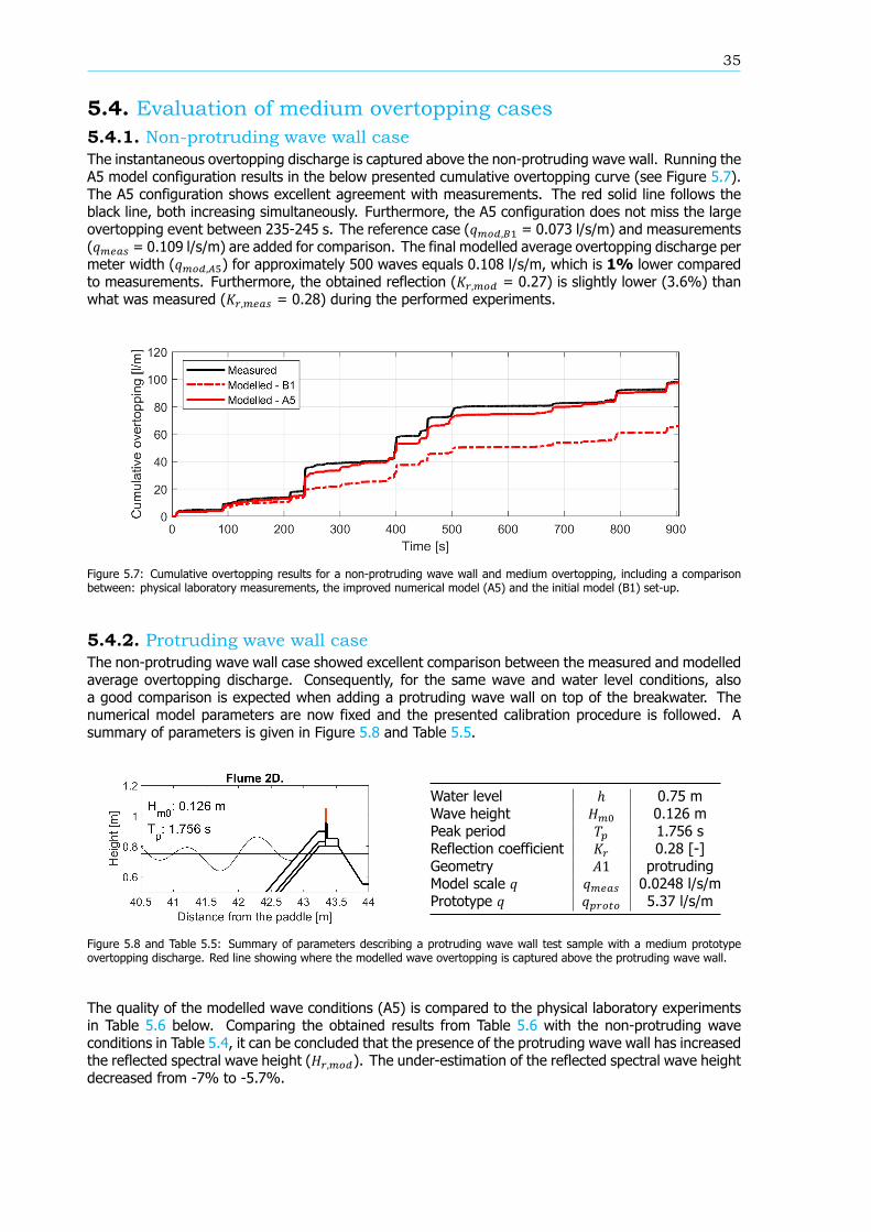
35

5.4. Evaluation of medium overtopping cases5.4.1. Non-protruding wave wall caseThe instantaneous overtopping discharge is captured above the non-protruding wave wall. Running theA5 model configuration results in the below presented cumulative overtopping curve (see Figure 5.7).The A5 configuration shows excellent agreement with measurements. The red solid line follows theblack line, both increasing simultaneously. Furthermore, the A5 configuration does not miss the largeovertopping event between 235-245 s. The reference case (𝑞 , = 0.073 l/s/m) and measurements(𝑞 = 0.109 l/s/m) are added for comparison. The final modelled average overtopping discharge permeter width (𝑞 , ) for approximately 500 waves equals 0.108 l/s/m, which is 1% lower comparedto measurements. Furthermore, the obtained reflection (𝐾 , = 0.27) is slightly lower (3.6%) thanwhat was measured (𝐾 , = 0.28) during the performed experiments.

Figure 5.7: Cumulative overtopping results for a non-protruding wave wall and medium overtopping, including a comparisonbetween: physical laboratory measurements, the improved numerical model (A5) and the initial model (B1) set-up.

5.4.2. Protruding wave wall caseThe non-protruding wave wall case showed excellent comparison between the measured and modelledaverage overtopping discharge. Consequently, for the same wave and water level conditions, alsoa good comparison is expected when adding a protruding wave wall on top of the breakwater. Thenumerical model parameters are now fixed and the presented calibration procedure is followed. Asummary of parameters is given in Figure 5.8 and Table 5.5.

Water level ℎ 0.75 mWave height 𝐻 0.126 mPeak period 𝑇 1.756 sReflection coefficient 𝐾 0.28 [-]Geometry 𝐴1 protrudingModel scale 𝑞 𝑞 0.0248 l/s/mPrototype 𝑞 𝑞 5.37 l/s/m

Figure 5.8 and Table 5.5: Summary of parameters describing a protruding wave wall test sample with a medium prototypeovertopping discharge. Red line showing where the modelled wave overtopping is captured above the protruding wave wall.

The quality of the modelled wave conditions (A5) is compared to the physical laboratory experimentsin Table 5.6 below. Comparing the obtained results from Table 5.6 with the non-protruding waveconditions in Table 5.4, it can be concluded that the presence of the protruding wave wall has increasedthe reflected spectral wave height (𝐻 , ). The under-estimation of the reflected spectral wave heightdecreased from -7% to -5.7%.

36 5. Model validation

Type Total In Reflected

Case RMSE [m] PCC [%] 𝐻 [%] RMSE [m] PCC [%] 𝐻 [%] RMSE [m] PCC [%] 𝐻 [%]A5 0.0149 91.68 -3.80 0.0123 93.14 -4.01 0.0049 85.97 -5.73

Table 5.6: Statistical and spectral parameters (RMSE, PCC and ) describing the quality of the wave conditions at wavegauge 5, including a comparison between: the improved numerical model (A5) in terms of total, incoming and reflected waveconditions.

When considering the incoming wave conditions, one would expect that the incident wave height wouldbe equal in both cases (as an identical steering file is used). However, a small dissimilarity is seen.The non-identical total surface elevation combined with the adopted reflection analysis method canintroduce such small differences. The total modelled spectral wave height decreased, which is mainlycaused by the reduction of the incoming wave conditions from -3.8% to -4.0%.

Figure 5.9 shows the comparison between the A5 modelled cumulative overtopping curve and mea-surements. Between 0 and 500 seconds an excellent comparability is found, represented by almostmatching lines. However, the difference between the measured (𝑞 = 0.033 l/s/m) and modelledovertopping quantities (𝑞 , = 0.043 l/s/m) is larger compared to the non-protruding case. Themeasured average overtopping discharge is over-estimated by 27.7%. It can therefore be concludedthat the cause lies in some overtopping events which have been modelled, but not measured (seeFigure 5.9). Additionally, the obtained reflection (𝐾 , = 0.28) can be considered equal to what wasmeasured (𝐾 , = 0.28) during the performed experiments.

Figure 5.9: Cumulative overtopping results for a protruding wave wall and medium overtopping, including a comparison between:physical laboratory measurements and the improved numerical model (A5).

Over the whole considered time series small overtopping events, referred to as overtopping discrepan-cies, are captured within the numerical model, resulting in sloping lines instead of horizontal lines (e.g.between 120-240 s and 240-400 s). Several causes can be identified:

∘ Wave conditions: discrepancies between modelled and measured total surface elevation timeseries at wave gauge 5, caused by a combination of:

• The incoming surface elevation time series, generated using the exterior OceanWaves3Dmodel. The frequency dependent amplification factor applied to the incoming wave condi-tions (see the calibration procedure in Section 5.3.1) improved the comparison in terms ofincoming spectral wave height (𝐻 , ) between the model and measurements. However,small differences still arise between the measured and modelled incoming surface elevationtime series (see Figure 5.6a, Section 5.3.1).

• The reflected surface elevation time series, which depends on the porous flow properties(reflection) of the breakwater. If the reflection induced by the breakwater is different fromwhat is experienced in the physical flume, a different reflected surface elevation is capturedat wave gauge 5.

37

Differences in the captured total surface elevation at wave gauge 5 could result in dissimilaritiesin overtopping discharges.

∘ Porous flow coefficients: the chosen coefficients (𝑛 (porosity), 𝛼, 𝛽 and 𝐾𝐶) in Section 5.3.2directly influence the overflow, wave breaking patterns and therefore the overtopping. The in-fluence on the overtopping is studied in Section 5.5.2. Nevertheless, the porous flow coefficientswere chosen based on a comparison of modelled and measured reflection coefficients (based onspectral wave heights 𝐻 ), not considering overflow over the breakwater.

∘ Degree of openness of the wave wall: a ventilated boundary is applied to the front of the wavewall, characterised by a degree of openness. A low degree of openness means that the wave wallis less permeable. As a consequence more water is pushed in upward and backward direction,which results in more wave overtopping and an increase in bulk reflection. The influence of theopenness of the wave wall on the average overtopping discharge is discussed in Section 5.5.3.

∘ Numerical diffusion in the overtopping region due to grid size: small overtopping events can beover-estimated when a coarse grid is applied in the capturing region (above wave wall). Smalldrops of water can be stretched out over the coarse cell, over-estimating the initial volume of thedrop. This cause is further elaborated in Section 5.5.4.

However, without flow measurements over the crest of the breakwater the first cause can not besubstantiated and is left for future research. The last three are addressed in the sensitivity analysis. Itis worth noting that the first two causes and the last cause also apply to the non-protruding wave wallcases.

5.4.3. Evaluation of individual overtopping eventsIn previous sections the cumulative overtopping curves were compared in terms of average discharges.Here, the individual modelled and measured overtopping events for both non-protruding and protrud-ing wave wall samples are compared; results are shown in Tables 5.7 and 5.8. The six largest measuredindividual overtopping events (O1-O6; see Figure 5.10) are compared in magnitude with model out-comes.

Figure 5.10: Cumulative measured overtopping results for a non-protruding wave wall and medium overtopping, showing thesix considered individual overtopping events.

Non-protruding wave wallThe A5 configuration shows improved results compared to the initial B1 configuration in case of a non-protruding wave wall (see Table 5.7). The individual volumes are under-estimated (14%) in the non-protruding wave wall case. Yet, the average overtopping discharge (see Section 5.6) showed excellentagreement with the measurements. In regions where the measurements show no overtopping events,the model captures very small overtopping events (overtopping discrepancies), which compensate theunder-estimated individual volumes.

38 5. Model validation

Event 𝑇 [s] 𝑉 [l/m] 𝑉 , [l/m] Error [%] 𝑉 , [l/m] Error [%]O1 91 - 95 4.4 2.4 -45.5 3.8 -13.6O2 237 - 241 12.6 4.5 -64.3 11.3 -10.3O3 396 - 399 5.2 2.9 -44.2 3.6 -30.8O4 399 - 402 9.5 5.8 -38.9 5.8 -38.9O5 455 - 459 6.2 3.8 -38.7 5.6 -9.7O6 882 - 886 5.1 3.5 -31.4 6.0 +17.6Mean - - - -43.8 - -14.3Std - - - ±10.2 - ±17.9

Table 5.7: Individual overtopping volumes (O1-O6) for the non-protruding wave wall with medium prototype overtopping case,including a comparison between: the measurements, the initial model (B1) and the improved model (A5) set-up.

Protruding wave wallThe A5 configuration shows good comparability with measurements, under-estimating the individualvolumes by 4% (see Table 5.8). The protruding wave wall average overtopping discharge was over-estimated (see Section 5.4.2). This over-estimation is caused by a combination of under-estimatedindividual volumes which are compensated by small overtopping discrepancies, as discussed for thenon-protruding wave wall case. However, the relative importance of these small overtopping discrepan-cies increases as the average overtopping discharge decreases due to the presence of the protrudingwave wall. Consequently, the average overtopping discharge for the protruding wave wall case isover-estimated.

Event 𝑇 [s] 𝑉 [l/m] 𝑉 , [l/m] Error [%]O1 91 - 95 1.9 1.4 -26.3O2 237 - 241 6.7 6.3 -6.0O3 396 - 399 1.8 1.7 -5.6O4 399 - 402 3.9 3.4 -12.8O5 455 - 459 2.5 2.8 12.0O6 882 - 886 1.3 1.5 15.4Mean - - - -3.9Std - - - ±14.2

Table 5.8: Individual overtopping volumes (O1-O6) for the protruding wave wall with medium prototype overtopping case,including a comparison between: the measurements and the improved model (A5) set-up.

39

5.5. Sensitivity analysisEach input parameter influences the overtopping results by a certain degree. Three uncertain parame-ters are studied below: the 𝐷 of the core of the breakwater, the porous flow resistance coefficients(𝛼, 𝛽 and KC) and the degree of openness of the wave wall. Additionally, the numerical diffusion inthe overtopping region is addressed.

5.5.1. 𝐷 of the coreFor the physical model construction, four different batches were used to built up the core of thebreakwater in the physical flume. Each batch is characterised by a grading curve and a 𝐷 (seeFigure 5.11), which relates to varying bulk reflections. Batches 1 and 4 represent both extremities:left and right compared to the average line. The nominal diameters (𝐷 ) for batches 1 and 4 are 5.7mm and 7.5 mm respectively (𝐷 = 0.84⋅𝐷 (CIRIA et al., 2007b)).

Figure 5.11: Four different batches were used to construct the core of the breakwater in the physical flume. All four sieve curvesare plotted against each other. The gradings ( ) and porosities ( ) of batches 1, 4 and average are modelled in OpenFOAM.

Using the same procedure as explained in Section 5.3.2 the found porosities are: 𝑛 = 0.430 and𝑛 = 0.417. Three runs are performed in OpenFOAM: batch 1, batch 4 and batch average run. Thefound reflection coefficients are: 𝐾 , = 0.28, 𝐾 , = 0.28 and 𝐾 , = 0.27. The averagecharacteristics of the core were used for the calibration runs (see Section 5.3.2 above). The overtoppingwas modelled during these runs (300 waves). The sensitivity analysis reveals that the discharge isnot affected by the value of 𝑛 and 𝐷 of the considered batches (see Figure 5.12). However, themagnitude of the individual overtopping events showed differences along the three modelled runs.

Figure 5.12: Cumulative overtopping results for a non-protruding wave wall and medium overtopping, including a comparisonbetween three numerical model runs (batch 1, batch 4 and batch average) with varying core characteristics ( and ).

40 5. Model validation

5.5.2. Porous flow resistance coefficientsAs shown earlier in Section 5.3.2 the dimensionless porous flow coefficients do influence the bulkreflection of the breakwater. Additionally, the wave and flow properties in front (e.g. wave breaking)and over the breakwater are also influenced by the choice of dimensionless porous flow coefficients.Numerous runs were done with varying dimensionless porous flow coefficients (see Section 5.3.2, Table5.3 above). The cumulative overtopping curves of the performed runs are reported in Figure 5.13.

Figure 5.13: Cumulative overtopping results for a non-protruding wave wall and medium overtopping, including a comparisonbetween four numerical model runs with varying porous flow coefficients ( and ) and ).

The original Jacobsen et al. (2018) run was left out for comparison since no change was made to thedimensionless resistance coefficients compared to the re-evaluated 𝐷 and 𝑛 run, where 𝛼 = 1,000,𝛽 = 1.1 and 𝐾𝐶 = 10,000. The remaining runs (see Figure 5.13) were performed using varying 𝛼 and𝛽 coefficients, keeping 𝐾𝐶 constant (which was calculated using Equation 4.6; see Chapter 4, Section4.3.3). Comparing the Losada et al. (2008) run with the Vanneste and Troch (2015) run reveals theinfluence of changing 𝛼 and 𝛽 coefficients on the cumulative overtopping curve (as 𝐾𝐶 is unchanged).It can be deduced that for increasing bulk reflection of the breakwater (less permeable) the averageovertopping discharge increases. The highest reflection coefficient was found using the proposed coef-ficients by Vanneste and Troch (2015) (𝐾 = 0.36), showing the highest average overtopping discharge(𝑞 = 0.07 l/s/m). As the breakwater is made less permeable, the flow of water over the crestof the breakwater is less capable to seep through the armour, filter layer and the core, which results inhigher overtopping quantities. The re-evaluated 𝐷 and 𝑛 run (𝐾 = 0.35) has a similar bulk reflectionto the Vanneste and Troch (2015) run. Nonetheless, the average overtopping discharge (𝑞 = 0.05l/s/m) is different. On the other hand, the Losada et al. (2008) and Jensen et al. (2014) runs showthe same comparability in terms of bulk reflection and similar average overtopping discharges. Thisshows how sensitive the dimensionless porous flow coefficients are in correctly capturing the overflowand eventually the wave overtopping over breakwaters.

5.5.3. Openness of the wave wallHere, the sensitivity of the degree of openness of the wave wall is analysed. The degree of opennessof the wave wall was introduced by Jacobsen et al. (2018) to compensate the over-predicted lift forcesdue to air entrapment upon wave breaking (see Section 4.5). Jacobsen et al. (2018) performed thevalidation of forces using values ranging between 0.5-6% and concluded that the 3% performed best.Here, two protruding wave wall cases are modelled in OpenFOAM with varying degree of openness ofthe wave wall (lower limit 0.5% and the optimal 3%). Two cases were esteemed enough to test thesensitivity of this parameter on the cumulative overtopping curve. As shown in Figure 5.14 below, itcan be concluded that a lower degree of openness (red line) results in a higher average overtoppingdischarge (42.7% higher). The front wall is made less permeable (from 3% to 0.5%), which pushesthe water flow in upward direction as the flume is two dimensional. The latter causes the increase inindividual overtopping volumes.

41

Figure 5.14: Cumulative overtopping results for a protruding wave wall and medium overtopping, including a comparison betweentwo numerical model runs with varying degree of openness of wave wall (0.5% and 3% degree of openness).

5.5.4. Numerical DiffusionUsing coarse meshes (overtopping region) to model small (splashes) overtopping events can inducenumerical diffusion. The water droplets are smaller than the considered grid cell and are stretchedout over the cell. The relative importance of these overtopping discrepancies increases with: loweraverage overtopping discharges and protruding wave wall cases. The presence of the protrudingwave wall, upon which the overflow impacts, generates splashes which are over-estimated due tothe coarse grid. This increases the amount of small overtopping events compared to non-protrudingwave wall cases and partly explains the over-estimations found for the protruding wave wall casecompared to the non-protruding wave wall case. Considering all the aforementioned, a protrudingsmall prototype overtopping case is expected to show the largest effect of this numerical diffusion. Inthis section an extra run is performed where the grid size resolution is increased (3x in the overtoppingregion, from 0.0125 m to 0.0016). From figure 5.15 below it can be inferred that, compared tomeasurements, the numerical model with refined overtopping region showed a reduction in overtoppingdiscrepancies, visible between 100 and 200 seconds. However, the computational effort required tocope with the higher grid size resolution increased with a factor 2.3x (from 61 hours to 141 hours),which is not desired. Therefore, the aforementioned over-estimation of small overtopping events isaccepted for medium and large prototype overtopping cases. To model small overtopping cases (bothnon-protruding and protruding) it is recommended to use an adequate grid in the overtopping region.Yet, due to time constraints, this was not carried out in the present research for the small overtoppingcases.

Figure 5.15: Cumulative overtopping results for a protruding wave wall and small overtopping, including a comparison between:the improved numerical model (A5) and the improved numerical model with an increased resolution (3x) in the overtoppingregion and measurements.

42 5. Model validation

5.6. Evaluation of large overtopping cases5.6.1. Non-protruding wave wall caseIn Section 5.3 above a calibration procedure was proposed based on a medium non-protruding proto-type overtopping discharge case. Here, the calibration procedure is evaluated for a large non-protrudingwave wall prototype overtopping discharge case. The wave conditions and geometry are shown in Fig-ure 5.16 and Table 5.9.

Water level ℎ 0.75 mWave height 𝐻 0.144 mPeak period 𝑇 1.461 sReflection coefficient 𝐾 0.21 [-]Geometry 𝐴3 non-protrudingModel scale 𝑞 𝑞 0.194 l/s/mPrototype 𝑞 𝑞 42.181 l/s/m

Figure 5.16 and Table 5.9: Summary of parameters describing a non-protruding wave wall test sample with a large prototypeovertopping discharge. Red line showing where the modelled wave overtopping is captured above the non-protruding wave wall.

The comparison between modelled and measured wave conditions is given in Table 5.10. A comparableaccuracy compared to the calibration case is attained, except for the reflected wave conditions whichover-estimate the measurements. This is in line with the modelled reflection coefficient (𝐾 , =0.22), which is higher (4.8%) than measured (𝐾 , = 0.21).

Type Total In Reflected

Case RMSE [m] PCC [%] 𝐻 [%] RMSE [m] PCC [%] 𝐻 [%] RMSE [m] PCC [%] 𝐻 [%]A5 0.0166 90.56 -1.77 0.0139 92.46 -2.90 0.0050 79.46 1.33

Table 5.10: Statistical and spectral parameters (RMSE, PCC and ) describing the quality of the wave conditions following theproposed validation process, for a non-protruding test sample with a large prototype overtopping discharge.

The modelled average overtopping discharge per meter width (𝑞 , ) for approximately 500 wavesequals 0.210 l/s/m, which is 2.5% higher compared to measurements (𝑞 = 0.205 l/s/m), as shownin Figure 5.17.

Figure 5.17: Cumulative overtopping results for a non-protruding wave wall and large overtopping, including a comparisonbetween: physical laboratory measurements and the improved numerical model (A5).

From Figure 5.17 it can be inferred that the model is capable of modelling large prototype overtoppingdischarges for the breakwater with non-protruding wave wall. An excellent comparison is seen be-tween the A5 configuration and the measured cumulative overtopping line over the whole time series,meaning that the individual events are well captured by CoastalFOAM. However, the model captures

43

small overtopping events which are not measured between 220-320 seconds. As mentioned in Section5.4.2 above these discrepancies can be caused by various factors. Being the influence on the overallresult limited, this is accepted.

5.6.2. Protruding wave wall caseA protruding test sample with a large prototype overtopping discharge, characterised by the followinggeometrical and hydraulic parameters (see Figure 5.18 and Table 5.11) is presented and analysedherebelow.

Water level ℎ 0.75 mWave height 𝐻 0.144 mPeak period 𝑇 1.461 sReflection coefficient 𝐾 0.22 [-]Geometry 𝐴1 protrudingModel scale 𝑞 𝑞 0.052 l/s/mPrototype 𝑞 𝑞 11.32 l/s/m

Figure 5.18 and Table 5.11: Summary of parameters describing a protruding wave wall test sample with a large prototypeovertopping discharge. Red line showing where the modelled wave overtopping is captured above the protruding wave wall.

The statistical and spectral comparison between model and measurements is reported in Table 5.12.

Type Total In Reflected

Case RMSE [m] PCC [%] 𝐻 [%] RMSE [m] PCC [%] 𝐻 [%] RMSE [m] PCC [%] 𝐻 [%]A5 0.0173 89.87 -2.04 0.0145 91.55 -3.10 0.0049 80.16 2.22

Table 5.12: Statistical and spectral parameters (RMSE, PCC and ) describing the quality of the wave conditions following theproposed validation process, for a protruding test sample with a large prototype overtopping discharge.

The modelled reflection coefficient (𝐾 , = 0.22) is equal when compared to measurements (𝐾 ,= 0.22). An increase in reflected spectral wave height, caused by the protruding wave wall, is seen inTable 5.12. The under-estimation of the total spectral wave height increased as the incoming spectralwave height further reduced, which weights more than the increase in reflected spectral wave height.One would expect that the incident wave height would be equal in both cases (as an identical steeringfile is used). However, a non-identical total surface elevation combined with the adopted reflectionanalysis method (using LWT in intermediate water) can introduce such small differences.

Figure 5.19: Cumulative overtopping results for a protruding wave wall and large overtopping, including a comparison between:physical laboratory measurements and the improved numerical model (A5).

The modelled average overtopping discharge per meter width (𝑞 , ; see Figure 5.19 above) forapproximately 500 waves equals 0.110 l/s/m, which is 85.1% higher compared to measurements

44 5. Model validation

(𝑞 = 0.059 l/s/m). The modelled cumulative overtopping line shows good agreement with themeasurements. However, the previously addressed erroneous overtopping events between 220 to 320s are also visible in this case. It is worth noting that their relative importance and number increasedby the presence of the protruding wave wall, as previously discussed in Section 5.5.4, and eventuallyleads to the seen over-estimation of the average overtopping discharge.

5.7. Evaluation of small overtopping cases5.7.1. Non-protruding wave wall caseIn this section the calibration procedure is carried out for a small non-protruding wave wall prototypeovertopping discharge case, characterised by the following geometrical and hydraulic parameters (seeFigure 5.20 and Table 5.13).

Water level ℎ 0.75 mWave height 𝐻 0.105 mPeak period 𝑇 1.628 sReflection coefficient 𝐾 0.25 [-]Geometry 𝐴3 non-protrudingModel scale 𝑞 𝑞 0.052 l/s/mPrototype 𝑞 𝑞 2.11 l/s/m

Figure 5.20 and Table 5.13: Summary of parameters describing a non-protruding test sample with a small prototype overtoppingdischarge. Red line showing where the modelled wave overtopping is captured above the non-protruding wave wall.

The quality of the modelled wave climate compared to measurements is reported in Table 5.14.

Type Total In Reflected

Case RMSE [m] PCC [%] 𝐻 [%] RMSE [m] PCC [%] 𝐻 [%] RMSE [m] PCC [%] 𝐻 [%]A5 0.0093 95.10 -5.58 0.068 96.61 -4.90 0.0032 87.85 -6.60

Table 5.14: Statistical and spectral parameters (RMSE, PCC and ) describing the quality of the wave conditions following theproposed validation process, for a non-protruding test sample with a small prototype overtopping discharge.

The modelled reflection coefficient (𝐾 , = 0.25) is equal than what was measured (𝐾 , = 0.25)during the performed experiments. The incoming wave condition is under-estimated by 5%, the ac-cepted limit. The under-estimated reflected and incoming spectral wave height resulted in an overallunder-estimated total spectral wave height (-5.6%).

Figure 5.21: Cumulative overtopping results for a non-protruding wave wall and small overtopping, including a comparisonbetween: physical laboratory measurements and the improved numerical model (A5).

The modelled average overtopping discharge per meter width (𝑞 , ) for approximately 500 waves

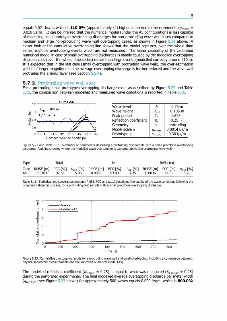
45

equals 0.021 l/s/m, which is 110.0% (approximately x2) higher compared to measurements (𝑞 =0.010 l/s/m). It can be inferred that the numerical model (under the A5 configuration) is less capableof modelling small prototype overtopping discharges for non-protruding wave wall cases compared tomedium and large non-protruding wave wall overtopping cases, as shown in Figure 5.21 above. Acloser look at the cumulative overtopping line shows that the model captures, over the whole timeseries, multiple overtopping events which are not measured. The lesser capability of the calibratednumerical model in case of small overtopping discharges is mainly caused by the modelled overtoppingdiscrepancies (over the whole time series) rather than large events (modelled correctly around 210 s).It is expected that in the last case (small overtopping with protruding wave wall), the over-estimationwill be of larger magnitude as the average overtopping discharge is further reduced and the wave wallprotrudes the armour layer (see Section 5.5.4).

5.7.2. Protruding wave wall caseFor a protruding small prototype overtopping discharge case, as described by Figure 5.22 and Table5.15, the comparison between modelled and measured wave conditions is reported in Table 5.16.

Water level ℎ 0.75 mWave height 𝐻 0.105 mPeak period 𝑇 1.628 sReflection coefficient 𝐾 0.25 [-]Geometry 𝐴1 protrudingModel scale 𝑞 𝑞 0.0014 l/s/mPrototype 𝑞 𝑞 0.30 l/s/m

Figure 5.22 and Table 5.15: Summary of parameters describing a protruding test sample with a small prototype overtoppingdischarge. Red line showing where the modelled wave overtopping is captured above the protruding wave wall.

Type Total In Reflected

Case RMSE [m] PCC [%] 𝐻 [%] RMSE [m] PCC [%] 𝐻 [%] RMSE [m] PCC [%] 𝐻 [%]A5 0.0103 92.54 -5.06 0.0086 93.43 -4.35 0.0036 84.95 -5.28

Table 5.16: Statistical and spectral parameters (RMSE, PCC and ) describing the quality of the wave conditions following theproposed validation process, for a protruding test sample with a small prototype overtopping discharge.

Figure 5.23: Cumulative overtopping results for a protruding wave wall and small overtopping, including a comparison between:physical laboratory measurements and the improved numerical model (A5).

The modelled reflection coefficient (𝐾 , = 0.25) is equal to what was measured (𝐾 , = 0.25)during the performed experiments. The final modelled average overtopping discharge per meter width(𝑞 , ; see Figure 5.23 above) for approximately 500 waves equals 0.009 l/s/m, which is 800.0%

46 5. Model validation

(approximately a factor 9) higher compared to measurements (𝑞 = 0.001 l/s/m). It can be deducedfrom the above that the numerical model (under the A5 configuration) is least capable of modellingsmall prototype overtopping discharges for protruding cases, as Figure 5.23 shows above. The modelledcumulative overtopping curve captures overtopping events where the measurements do not (straightline). As expected, the over-estimation is the most pronounced in this case; the small protrudingwave wall overtopping case amounts the lowest average overtopping discharge and is characterisedby the presence of the wave wall. The effect of numerical diffusion for this case was illustrated inFigure 5.15 (see Section 5.5.4 above), where the estimated average overtopping (under the A5 - 3xrefined configuration) discharge amounted 0.004 l/s/m, which is 311% higher than measured. This isan improvement compared to the earlier mentioned 800%. However, the run is disregarded for futurecomparison since it consisted of a different grid in the overtopping region compared to other runs anddid not account for 500 waves. Nonetheless, from the foregoing it can be concluded that an increasedgrid resolution is required to accurately model small overtopping protruding wave wall cases at the costof computational time.

5.8. SummaryHerebelow a summary is given of the obtained numerical model results (CoastalFOAM; considering 500waves), which are compared with measurements. To compare the results the EurOtop 2018 proposes toplot the relative overtopping rate (𝑞/(𝑔𝐻 ) . ) against the relative freeboard (𝑅 /𝐻 ). The format ofFigures 5.24 and 5.25 is based on Figure 6.7 of the EurOtop manual 2018. For the spectral wave height(𝐻 ) the measured incident spectral wave height is used, since the difference in incident spectral waveheight between the calibrated numerical model and measurements was minimal.

Non-protruding wave wallFor the non-protruding wave wall cases (see Figure 5.24), CoastalFOAM showed good agreement withmeasurements.

Figure 5.24: Mean overtopping discharge for non-protruding wave wall cases in terms of relative overtopping rate and relativefreeboard, including a comparison between: physical laboratory measurements, the improved numerical model (CoastalFOAM).

The calibration procedure from the original model configuration (B1) to the A5 configuration showedimproved results in terms of wave conditions, overtopping discharges and individual overtopping vol-umes for both the medium and large overtopping case. All this resulted in improved comparability withmeasurements for the medium and large overtopping cases (two left data points) compared to thesmall overtopping case.

Protruding wave wallWhen considering the protruding wave wall cases (see Figure 5.25 below), it can be deduced thatCoastalFOAM over-estimated the measurements for all cases. For two (medium and large overtopping)

47

out of three cases the model showed good agreement with measurements. Two causes were workedout for the over-estimated model outcomes compared to measurements:

∘ The overtopping discrepancies (see Section 5.5.4 above), which became more frequent for pro-truding wave wall cases and relatively more important for decreasing average overtopping dis-charge (to the right in Figure 5.25).

∘ The degree of openness of the wave wall, which has a significant influence on the averageovertopping discharge, as seen in Section 5.5 above.

Therefore, when modelling small overtopping with protruding wave wall cases, it is recommended toincrease the resolution of the grid in the overtopping region.

Figure 5.25: Mean overtopping discharge for protruding wave wall cases in terms of relative overtopping rate and relativefreeboard, including a comparison between: physical laboratory measurements and CoastalFOAM.

Finally, the accuracy of the calibrated model (CoastalFOAM; A5 model set-up) is evaluated againstthe accuracy achieved by the uncalibrated version of the numerical model, applied by Boersen et al.(2019), considering the average overtopping discharge as evaluation criterion. Eight overtopping caseswere selected and modelled by Boersen et al. (2019). Out of the eight cases, six are selected herefor the comparison (small, medium and large overtopping with non-protruding and protruding wavewall cases). The cases modelled by Boersen et al. (2019) are not equal to the ones modelled in thisresearch, hence the reported difference in measured average overtopping discharges in Table 5.17.The comparison is done (see Table 5.17) in terms of RMSE (l/s/m) relative to the measured averages,where the calibrated model shows improved results for both non-protruding and protruding wave wallcases. The RMSE values relative to the measured averages are lower for CoastalFOAM (non-protruding= 0.07, protruding = 0.97) compared to the uncalibrated model (non-protruding = 0.16, protruding =1.67) for both geometries.

Non-protruding Protruding[l/s/m]

Measured average (Boersen et al., 2019) 0.106 0.027Measured average 0.108 0.031

RMSE [l/s/m]Uncalibrated (Boersen et al., 2019) 0.017 0.045CoastalFOAM 0.008 0.030

Table 5.17: Measured average discharges and RMSE values when applying the uncalibrated model or CoastalFOAM for theestimation of the average overtopping discharge , including a separation between protruding and non-protruding wave wallcases.

6Model application

6.1. IntroductionIn this chapter the focus shifts from average overtopping discharges (𝑞), validated in Chapter 5, tomaximum overtopping volumes (𝑉 ). First, the definitions of extreme wave and overtopping eventsadopted in the present research are given. Second, the reasoning and the advantages of the proposedshift are explained. Third, a theory is elaborated where the surface elevation of extreme wave eventsis reconstructed based on spectral wave properties of a given sea state. The following topics will beaddressed for clarification: wave focusing, the NewWave theory, its application in the coastal engineer-ing domain and the first order wave generation. Finally, two methodologies are presented in whichthe NewWave theory is applied numerically (using CoastalFOAM) to assess: maximum overtoppingvolumes and average overtopping discharges based on the spectral wave properties at the toe of thebreakwater.

6.1.1. Extreme wave and overtopping eventsIn the present research an extreme wave event is defined as: a train of waves containing the highestwave of the considered sea state, which is characterised by its spectral parameters (𝐻 , 𝑇 and thepeak enhancement factor 𝛾). The waves prior to the highest wave are also considered to be part of theextreme wave event. These preceding waves ”warm-up” the rubble mound breakwater, i.e. running upand down the slope which reduces the roughness (filling of pores armour or filter layer) for upcomingwaves. Furthermore, an extreme overtopping event is defined as: the wave overtopping volumecaptured during the interaction between the extreme wave event and the rubble mound breakwater.

6.2. Importance of the maximum overtopping volumeIn Chapter 5 the numerical model was validated for the reproduction of average overtopping dischargesover rubble mound breakwaters. Nevertheless, the average overtopping discharge as a quantity is notcapable of identifying extreme overtopping events. It gives the total overtopped volume over the con-sidered period. However, extreme events are likely to cause most of the damage to coastal structures,as suggested by Franco et al. (1994), using the largest individual overtopping volume instead of anaverage value for design. The EurOtop 2018 manual mentions that most damage close to the hydraulicstructure is caused by the largest overtopping volumes. For a given mean overtopping discharge, smallwaves will produce small overtopping volumes. On the other hand, large waves carry many cubic me-ters of overtopping water in one wave. Therefore, tolerable limits should also be based on overtoppingvolumes and not only on tolerable mean discharges.

To highlight this further, the 54 performed laboratory experiments for a protruding and non-protrudingwave wall on top of a rubble mound breakwater are shown in Figure 6.1.

49

50 6. Model application

Figure 6.1: Maximum volumes plotted against the average discharges for the respective cases, 27 protruding wave wall casesand 27 non-protruding wave wall cases.

For each case, the measured maximum overtopped volume is plotted against the measured averageovertopping discharge. The former is estimated from the available measured cumulative overtoppingcurves. The maximum vertical increment over a period of 1⋅𝑇 is defined as the maximum overtoppingvolume (see Figure 6.2).

Figure 6.2: Technique to estimate the maximum overtopped volume from the measured cumulative overtopping curves.

According to the EurOtop 2018 guidelines the highest average overtopping discharge would be used toevaluate the height of the rubble mound breakwater. In Figure 6.1, the case with the highest overtop-ping discharge is visualised by the intersection of the blue dotted lines and is characterised by a 𝐻 =0.123 m, 𝑇 = 2.26 s with a water level equal to 0.80 m (case A3W1T103 in Table A.1). Nonetheless,the last mentioned case does not contain the highest overtopped volume. Cases with higher maximumovertopped volumes, compared to case A3W1T103, are circled in red as the EurOtop does not considerthem for design purposes. Yet, the red circled cases could induce more damage to the rubble moundbreakwater.

Two situations can be distinguished when designing a rubble mound breakwater: the ServiceabilityLimit State (SLS) and the Ultimate Limit State (ULS). The SLS is the design to ensure that the structureis suitable for its use, whereas the ULS is the design to ensure that the structure is safe and does notfail under high loads. In both approaches, the maximum overtopping volume can be used as designstandard, admitting that the ULS probably has a higher (acceptable) overtopping volume than the SLS.For the ULS the overtopping volume required to damage the breakwater would be considered. On theother hand, for the SLS the overtopping volume (hydrodynamics) causing pedestrians’ their instabilitywhen walking over a breakwater can be used, as done by Arrighi et al. (2017) for floodwaters. Instead

51

of looking at a full sea state to assess the individual overtopping volumes (see Chapter 5 above), com-pact extreme wave and overtopping events will be reproduced and compared with empirical methodsand measurements. From a numerical point of view, simulating compact extreme wave events is anattractive solution as it would reduce simulation times. This opens up the possibility to increase theamount of set-ups that could be tested. The generation of extreme wave events is discussed next.

6.3. Focused wave groupExtreme wave events arise due to four different processes: wave-current interaction, wave-bottominteraction (shoaling), wave-wind interaction and wave-wave interaction (i.e. linear superposition andphasing of multiple wave components). The latter process will be considered as wave focusing. Thesurface elevation can be expressed as a linear superposition of multiple independent harmonic compo-nents (see Equation 6.1), at any point in space and time.

𝜁(𝑥, 𝑡) = ∑𝑎 𝑐𝑜𝑠(𝑘 𝑥 − 𝜔 𝑡 + 𝜙 ) (6.1)

Where 𝑁 is the number of wave components considered to recreate the focused wave group, 𝑥 is thehorizontal distance from the wave paddle, 𝑡 is time, 𝑎 is the wave amplitude, 𝑘 the wave number,𝜔 the angular frequency and 𝜙 the phase of the 𝑛 component. In case of an irregular sea state,for each wave component the 𝜙 would be randomly distributed between 0 and 2𝜋. However, informulating a focused wave group this phase is not random. When the waves are focused at a certainlocation 𝑥 and time 𝑡 , the phase 𝜙 of each component satisfies Equation 6.2. Combining Equations6.1 and 6.2 results in Equation 6.3.

𝜙 = −𝑘 𝑥 + 𝜔 𝑡 + 2𝑚𝜋, 𝑚 = 0,±1,±2, ... (6.2)

𝜁(𝑥, 𝑡) = ∑𝑎 𝑐𝑜𝑠(𝑘 (𝑥 − 𝑥 ) − 𝜔 (𝑡 − 𝑡 )) (6.3)

Upon focusing, constructive interference occurs among the considered wave components, which resultsin a large energetic event (extreme wave event). The focusing only occurs at 1 location, namely 𝑥 ; atother locations the maximum surface elevation is less. For that reason, the choice of the focus locationwill be substantiated as it is expected to have a significant influence on the overtopping results.

6.4. The NewWave theoryThe NewWave theory by Tromans et al. (1991) opens up the possibility to define the extreme waveevent from a wave spectrum. The surface elevation of the extreme wave event created with theNewWave theory is referred to as: NewWave profile. A NewWave profile is consistent with the math-ematical description of the expected shape of extreme wave events in a linear random sea, as shownby Jonathan and Taylor (1995).

The underlying statistical theory originates from Lindgren (1970), who described the expected (mostprobable) shape near an arbitrary crest with a non-linear relation. However, when the crest height isincreased (extreme wave events) the Lindgren profile converges to a linear relation, 𝑎 ⋅ 𝑟 , which is thescaled auto-correlation function and where 𝑟 is the autocorrelation function for the Gaussian surfacein time and 𝑎 the surface elevation.

This asymptotic solution is applied in this research. The theory is valid when the wave amplitudeof the NewWave profile is large compared to the standard deviation of the considered process (surfacedeviation). According to the NewWave theory the profile is given by the normalised auto-correlationfunction pre-multiplied with crest height of interest (𝜂 ). The crest-focused NewWave profile timeseries is given by Equation 6.4 herebelow.

𝜁(𝑡) = 𝜂∑ 𝑆 (𝜔)Δ𝜔 𝑐𝑜𝑠(𝜔 (𝑡 − 𝑡 ))

∑ 𝑆 (𝜔)Δ𝜔 (6.4)

52 6. Model application

Where 𝜂 is the desired amplitude of the NewWave profile at focus location which can be extractedfrom a wave height distribution fit to measured data, 𝑆 is the variance spectral density of the modelledunderlying wave energy spectrum (JONSWAP, Pierson Moskowits or others) and Δ𝜔 the angular fre-quency resolution. In Equation 6.4 the numerator is the auto-correlation function, given by the inverseFourier transform of the underlying spectrum. The denominator is the normalising factor, which is thevariance of the considered wave spectrum. By combining Equations 6.3 and 6.4 the individual waveamplitudes 𝑎 can be derived (see Equation 6.5) to obtain a desired NewWave profile at focus location.Filling in these individual wave amplitudes in Equation 6.3 gives the crest-focused NewWave profiletime series (see Equation 6.6).

𝑎 =𝜂 𝑆 (𝜔)Δ𝜔∑ 𝑆 (𝜔)Δ𝜔 (6.5)

𝜁(𝑡) = ∑𝑎 𝑐𝑜𝑠(𝜔 (𝑡−𝑡 )) = ∑𝜂 𝑆 (𝜔)Δ𝜔∑ 𝑆 (𝜔)Δ𝜔 𝑐𝑜𝑠(𝜔 (𝑡−𝑡 )) = 𝜂

∑ 𝑆 (𝜔)Δ𝜔 𝑐𝑜𝑠(𝜔 (𝑡 − 𝑡 ))∑ 𝑆 (𝜔)Δ𝜔

(6.6)Several input parameters are therefore needed for the creation of a NewWave event at 𝑥 . The waveamplitudes are based on the underlying spectrum properties. The essential parameters to recreate aNewWave are listed below:

∘ 𝜂 : the desired surface elevation at focusing point [m]

∘ 𝛾: peak enhancement factor [-]∘ 𝑇 : peak period [s]∘ 𝑥 : location of focusing [m]∘ 𝑡 : time of focusing [m]∘ 𝑓 : lower cut-off frequency [Hz]

∘ 𝑓 : higher cut-off frequency [Hz]

6.4.1. The NewWave theory in coastal engineeringThe NewWave profile has been applied as design wave in the coastal engineering domain. Offshoreconditions (wave spectrum) are analyzed and transformed nearshore using numerical models (e.g.SWAN). The nearshore spectral wave properties are used as input for the NewWave theory, generatingthe NewWave profile. The latter is modelled numerically to study which responses coastal structures(e.g. quay walls; Antonini et al. (2017)) give under extreme conditions. Hofland et al. (2014) cre-ated multiple NewWave profiles. They extracted 𝜂 from the probability of exceedance curve ofthe measured wave heights. The captured overtopping volumes were compared with the measuredovertopping volumes. The NewWave profiles caused overtopping volumes which lied within a factor 2compared to measurements.

Recently Whittaker et al. (2016) demonstrated that the NewWave profile can be adopted in intermedi-ate and shallow waters. However, as waves in intermediate water depth are non-linear, adjustmentsare added to the NewWave profile, referred to as second order corrections.

Whittaker et al. (2018) studied extreme overtopping events over an inclined seawall on a sloping fore-shore. The overtopping due to a NewWave group showed a strong dependence on the focus location,the linear amplitude and the phase of the group at focus.

6.4.2. First order wave generationThe desired NewWave profile at focus location is given by Equation 6.4, while the amplitudes of thewave components in order to recreate the profile by Equation 6.5. Still, as the NewWave profile is tobe generated in OceanWaves3D (as input for CoastalFOAM), a wave paddle signal (horizontal velocitytime series) is needed to recreate the desired profile. The NewWave profile is transformed to the

53

paddle position with linear wave theory. Thereafter, a first order (linear) wave-maker theory is used togenerate the horizontal paddle displacement time series. The followed process is shown in Figure 6.3.A detailed description of the linear wave-maker theory is given by Dean and Dalrymple (1991) and isreferred to for more details.

Figure 6.3: Process to achieve the desired NewWave profile at focus location, including: the NewWave theory to compute theNewWave profile at focus location, the linear wave theory to transform the NewWave profile to the paddle and a first order wavegeneration to produce the necessary steering file.

6.5. Application of the NewWave theoryIn the present research the NewWave theory is applied in two different ways:

∘ (i) methodology to assess the maximum overtopping volume given the spectral properties at thetoe of the breakwater.

∘ (ii) methodology to assess the average overtopping discharge using the maximum overtoppingvolume as input.

These two applications are explained in the upcoming sections.

6.6. Methodology to assess the maximum overtopping volume(𝑉𝑚𝑎𝑥)

In the presented methodology the NewWave theory is used to create a NewWave profile based onspectral properties at the toe of the breakwater, addressed in Section 6.6.1. The NewWave profilerepresents the largest event in a given sea state, characterised by its wave spectrum and parame-ters. The methodology assesses the maximum overtopping volume caused by the interaction of thatNewWave profile with the hydraulic structure. The measured incoming spectral properties are used asinput parameters for the NewWave profile. This to ensure that the obtained overtopping volumes arecomparable with the maximum measured overtopping volumes for validation purposes. The method-ology is applied to 18 cases; non-protruding and protruding wave wall with a water depth (ℎ) of 0.75m (A3W1T201-A3W1T209 & A1W1T201-A1W1T209; see Appendix A). The required input parameters(see Section 6.4 above) for the NewWave profile are derived from the measurements. After this, theNewWave profile is modelled in OCW3D, where a comparison is made between the theoretical pro-file and the NewWave profile generated in OCW3D. Several iterations are required to ensure that the𝜂 and the focus location 𝑥 obtained in OCW3D are equal to the desired input values. Finally, theNewWave profile is modelled in CoastalFOAM to account to model the overtopping over the breakwater.

The followed methodology is summarized in a flowchart (as shown in Figure 6.4), and can be ap-plied in cases where the designer chooses the maximum overtopping volume as design criterion (firststep). All the proposed steps on the left and right of the orange box are steps required to recreate aNewWave profile which can be validated with measurements. The orange box represent the reprodu-cable methodology, where the input parameters for the NewWave profile are derived and chosen andthe maximum overtopping volume is obtained as output. To guide the reader trough the methodology,the respective steps are illustrated below in different sections.

54 6. Model application

Figure 6.4: Flowchart representing the followed methodology in order to obtain , for each case which is compared to, . Red colour representing MATLAB procedures, yellow numerical modelling in CoastalFOAM, purple measurements

and gray input parameters for the NewWave model.

55

6.6.1. Input parametersThe NewWave profile will be constructed for nine cases, each based on the measured incoming waveconditions. The latter are obtained using the Zelt and Skjelbreia (1992) reflection analysis method,with 5 wave gauges. The incoming surface elevation time series are transformed to wave spectra,from which spectral properties, such as 𝐻 , 𝑇 , 𝑓 and 𝑓 , can be extracted (see Figure 6.5).

(a) Spectrum of incoming wave signal. (b) Location of interest.

Figure 6.5: (a) Showing two possible spectrum fits applied to the incoming wave spectrum, where the JONSWAP ( = 3.3)showed a good comparison with the measured incoming spectrum. Grey lines showing the threshold cut-off limits and .(b) Location where the incoming measured wave spectrum was captured (wave gauge 5).

The peak enhancement factor is one of the required input parameters for the NewWave theory. Itcan be inferred that the JONSWAP fit shows good resemblance with the incoming surface elevationspectrum (case A3W1T205; see Appendix A). This resemblance is seen for all cases (see Section C.1,Appendix C). Therefore, a peak enhancement factor equal to 3.3 is chosen to construct the NewWaveprofiles (JONSWAP type), creating a wider extreme event compared to a Pierson-Moskowits spectrum(see Figure 6.6).

Figure 6.6: Comparison between two possible NewWave events depending on which enhancement factor ( ) is used and wherethe Pierson Moskowits NewWave profile shows an improved capacity of focusing compared to the JONSWAP NewWave profile.

This can be clarified by the groupiness of the wave energy around the peak period 𝑇 which is strongerin case of a JONSWAP spectrum, focusing the energy around a limited amount of discrete frequenciesavailable to reconstruct the NewWave group, as explained in Section 6.3 above. Combining a limitedamount of wave components, which do not vary much in wave celerity (energy focused around peak),results in a reduced capacity of focusing. Therefore the JONSWAP NewWave profile is characterised bya larger wave group compared to the Pierson-Moskowits NewWave profile. The cut-off frequency limits

56 6. Model application

are chosen as 0.2 Hz (lower cut-off) and 2 Hz (upper cut-off) for all cases, as the wave energy lieswithin these limits and the peak periods can be extracted from the measured incoming wave spectra.Important to note is that measurements have been carried out for approximately 1000 waves (rangingfrom 1094 to 1223 over nine cases). Therefore, the highest wave has a probability of exceedance of1/1000 = 0.1%. In this research a comparable NewWave profile is modelled (𝜂 = 𝜂 . %), making theobtained measured 𝑉 , comparable with the NewWave profile induced overtopping volumes(𝑉 ). The presented methodology is based on the assumption that no surface elevation timeseries are available; therefore, 𝜂 . % needs to be estimated based on spectral properties. This is doneso that the developed method can be reproduced in lack of surface elevation time series. The 𝜂 . %is obtained from a Composite Weibull distribution fit based on spectral properties as suggested byBattjes and Groenendijk (1999) and is therefore coupled to the wave spectrum. A Composite Weibulldistribution is chosen since the limited water depth (intermediate water depth), which could inducewave-breaking for wave heights above the threshold value (see Figure 6.7). In these cases the Rayleighdistribution is not valid anymore.

Figure 6.7: Composite Weibull exceedance curve for incoming wave heights considering case T205, showing a Rayleigh distri-bution (red line) until the threshold wave height and from there a Weibull distribution (red dotted line).

Data points are given as comparison, ensuring that values comparable to the measurements are ex-tracted from the fitted distribution. As a result, the comparison between CoastalFOAM-NewWave andmeasurements can be done. The proposed procedure to extract the 𝐻 . % based on spectral propertieswas developed by Battjes and Groenendijk (1999) and is briefly explained below. Three input variablesare of importance:

∘ water depth: ℎ∘ slope angle: 𝛼∘ spectral wave height: 𝐻

Two out of these three variables (ℎ and 𝐻 ) can be extracted from an offshore nearshore transfor-mation using SWAN or other numerical models. In this research the spectral wave height (𝐻 ) isderived from the reconstructed measured incoming spectrum after application of the reflection analy-sis method. The slope angle can be retrieved from bathymetry profiles, yet for the studied cases thebottom is flat and therefore 𝛼 is taken as a very large value (close to flat). The wave height whichdetermines the transition between the Rayleigh part (𝐻 < 𝐻 ) and the Weibull part (𝐻 > 𝐻 ) of theComposite Weibull distribution is called the transitional wave height and is determined by Equation 6.7.In case of a flat slope the second term can be discarded, as tan 𝛼 becomes zero. Furthermore, theroot means squared wave height is determined using Equations 6.8 and 6.9.

𝐻 = (0.35 + 5.8 ⋅ tan 𝛼) ⋅ ℎ (6.7)

𝐻 = (2.69 + 3.24 ⋅ Ψ)√𝑚 (6.8)

57

Ψ = √𝑚ℎ (6.9)

Now, the ratio between 𝐻 and 𝐻 determines the non-dimensional transitional wave height (ℎ̃ ),needed to determine �̃� and �̃� , using Table 7.1 in Appendix C as explained by Battjes and Groenendijk(1999). The aforementioned non-dimensional values are in turn used to obtain 𝐻 and 𝐻 , usingEquations 6.10 and 6.11, needed to complete the non-exceedance Composite Weibull distribution givenby Equation 6.12, where 𝑘 and 𝑘 equal 2 (Rayleigh) and 3.6 (Weibull) respectively.

𝐻 = �̃� ⋅ 𝐻 (6.10)

𝐻 = �̃� ⋅ 𝐻 (6.11)

𝐹(𝐻) ≡ 𝑃𝑟(𝐻 ≤ 𝐻){𝐹 (𝐻) = 1 − exp [− ( ) ] 𝐻 ≤ 𝐻

𝐹 (𝐻) = 1 − exp [− ( ) ] 𝐻 > 𝐻(6.12)

From Figure 6.7 above it can be deduced that the Composite Weibull wave height exceedance distribu-tion over-estimates the incoming measured wave heights, which increases for increasing non-linearity(increasing Ursell number) of the considered wave conditions. This over-estimation may be causedby the applied reflection analysis method (Zelt and Skjelbreia (1992)), which uses linear wave the-ory. This increased over-estimation for increasing non-linearity is shown in Section C.2 of Appendix C,where for all cases the Composite Weibull distribution is plotted against the incoming measured waveheights. Nevertheless, the wave heights extracted from the Composite Weibull distribution are highercompared to the measured incoming wave heights and can be accepted, since they give a safer de-sign compared to the situation where the wave height would be under-estimated. Table 6.1 gives theresulting 𝜂 . % using Battjes and Groenendijk (1999) technique. Additionally, the maximum measuredcrest elevations (𝜂 ), obtained after adopting the reflection analysis method with a zero-downcrossing method, are reported. This is done to show if the extracted 𝜂 . % values lie within acceptablerange when compared to the measured values, which is the case. The Ursell number for the NewWaveprofile is calculated using the 5 highest waves within each NewWave profile (obtained with a zero-downcrossing method).

Case H [𝑚] T [𝑠] h [m] 𝐻 . % [m] 𝜂 . % [m] 𝜂 [m] 𝜂 [m] 𝐿 [m] Ursell [-]

T201 0.106 2.16 0.75 0.195 0.098 0.111 0.007 5.22 6.30T202 0.124 2.36 0.75 0.230 0.115 0.120 0.013 5.82 8.84T203 0.138 2.53 0.75 0.257 0.129 0.141 0.018 6.32 11.70T204 0.104 1.66 0.75 0.192 0.096 0.100 0.002 3.68 3.47T205 0.126 1.81 0.75 0.233 0.117 0.116 0.007 4.16 5.18T206 0.148 1.97 0.75 0.271 0.136 0.139 0.013 4.65 7.79T207 0.101 1.32 0.75 0.186 0.093 0.094 0 2.58 1.52T208 0.123 1.46 0.75 0.229 0.115 0.113 0.002 3.04 2.41T209 0.144 1.56 0.75 0.266 0.133 0.138 0.003 3.40 3.70

Table 6.1: Spectral properties of the incoming measured/physical wave conditions for all considered cases. Based on thespectral wave height , the . % is found according to Battjes and Groenendijk (1999) used to construct the CompositeWeibull distribution from which . % is derived and compared to the maximum experienced during measurements.Additionally, for each case a degree of non-linearity has been given in terms of the Ursell number.

6.6.2. Comparison between the theoretical and the OceanWaves3D NewWaveprofile

A MATLAB script ”focusedwaves2.m” (applying the NewWave and linear wave theory with a first orderwave generation) is used to produce the NewWave profile based on spectral properties. A first-orderwave generation is used to compute the required horizontal paddle velocity time series. Using the𝜂 . %, 𝑇 , 𝛾 and 𝑥 as input variables does not immediately result in the desired NewWave profile at

58 6. Model application

the focus location on first try. Therefore, an iterative approach is opted where the 𝜂 . % and the focuslocation 𝑥 are changed until comparable results are achieved. An example of a NewWave profileobtained with the iterative approach is given in Figure 6.8, which shows that the modelled NewWaveprofile is different from the NewWave profile according to the NewWave theory. This difference couldaffect wave overtopping results and is discussed below.

(a) Focused wave group, wave climate T203. (b) Location of focusing.

(c) Focused wave group, wave climate T207. (d) Location of focusing.

Figure 6.8: Comparing the most non-linear NewWave focused wave group (a, b) with the least non-linear NewWave focusedwave group (c, d), where the spurious waves gain in magnitude for increasing non-linear character.

Using a first-order wave generation to produce a NewWave profile in intermediate water depths (weaklynon-linear waves) introduces errors, referred to as ”spurious waves” or ”error waves”. It is caused byusing the linear wave generation outside its validity range. The error waves consist of low frequencywaves travelling ahead of the NewWave profile and of high frequency waves trailing behind, as canbe seen in Figure 6.8a. A set-up is experienced ahead of the NewWave profile. The set-up 𝜂in front of the NewWave profile is quantified by subtracting the original (black) and the filtered signal(red dotted). This set-up (approximately 0.018 m for an input 𝜂 . % = 0.129 m; the highest amongall cases) is visible in Figure 6.9a below, where the long error wave is filtered out using a frequencycut-off filter for case T203 (most non-linear, highest Ursell number). The other remaining cases arereported in Sections C.3 and C.4 of Appendix C. The waves trailing behind will not influence the waverun-up and the overtopping results as they interact with the structure after the NewWave profile haspassed. Therefore, from now on these waves are not considered anymore.

In contrast, the long error wave does influence run-up levels and overtopping quantities as reported byOrszaghova et al. (2014) and Whittaker et al. (2017). The spurious wave enhances the wave heightsin front of the leading crest of the NewWave profile and flattens the troughs which induces later wavebreaking. Orszaghova et al. (2014) reported that the spurious wave reduced overtopping volumesbetween 25-83%. However, they were studying a sloping foreshore where waves do have the time tobreak before arriving at the structure. In this research, instead, the bed is horizontal and the distanceover which the waves tend to break small (armour slope). Therefore, the aforementioned effect on theovertopping quantities is expected to be less significant. The long error wave could be removed witha second order wave generation technique, as proposed by Schaffer (1995), but this is left for futureresearch.

It can be concluded from the reported figures in Section C.4 of Appendix C and the reported 𝜂in Table 6.1 that the magnitude of the produced spurious waves is correlated with the degree of non-

59

linearity of the produced NewWave profile. The higher the degree of non-linearity, given by the Ursellnumber, the more pronounced the spurious wave. The Ursell number is obtained by considering thewave height and period (wave length) of the 5 highest waves within the travelling NewWave profile.If the nine considered cases (T201-209) are ranked in function of the degree of non-linearity, andcompared between themselves, some conclusions can be derived. Looking at Table 6.1 above, caseT203 shows the highest degree of non-linearity (Ursell number). In contrast, Figure 6.9b (case T207)shows the least.

(a) Case T203.

(b) Case T207.

Figure 6.9: A comparison for case T203 (a) and T207 (b) between the NewWave profile containing the low frequency error wave(black line) and the NewWave profile where the low frequency wave is filtered out (red dotted line).

If both cases (T203 and T207) are plotted (see Figure 6.9), it can be concluded that for increasingnon-linearity (increasing Ursell number) the magnitude of the spurious waves increases and is mostpronounced for case T203. The comparison between the theoretical NewWave profiles and what isgenerated in OceanWaves3D for the other cases is reported in Section C.3 of Appendix C.

6.6.3. NewWave in CoastalFOAMThe produced NewWave profiles (capturing 𝜂 . % well at the desired focus location, 𝑥 ) are now mod-elled in CoastalFOAM to procure the maximum overtopping volumes 𝑉 . The NewWave profilesare modelled in CoastalFOAM with the same numerical settings used for the validation of the aver-age overtopping discharge. Figure 6.10 below shows the incoming wave climate (red) generated withOceanWaves3D and the total surface elevation (black) measured at focusing point close to the toe of thebreakwater. The difference between the OceanWaves3D and the CoastalFOAM signal is caused by thepresence of the structure in the CoastalFOAM domain, inducing reflection. The reflection coefficientsfor all 9 cases have been computed and lie within a 6% confidence interval when compared to mea-sured reported reflection coefficients from the full time series. Reflection is therefore well representedusing the corrected porous flow coefficients (see Chapter 5).

60 6. Model application

(a) Surface elevation time series. (b) Location of interest.

(c) Overtopping discharge time series. (d) Measuring location.

Figure 6.10: (a) Comparison between CoastalFOAM and OceanWaves3D surface elevation time series for a non-protruding wavewall case, where the difference is induced by the reflection of the rubble mound breakwater. (b) The location at which thecomparison is made. (c) The instantaneous overtopping discharge caused by the NewWave. (d) The location at which theovertopping discharge is captured.

The distance between the wave gauge at which the focusing occurs and the measuring overtoppingsurface (model) is roughly 2.2 m. The time at which the 𝜂 . % passes is measured at 212.9 s and thetime at which the peak overtopping discharge is captured occurs around 214.0 s, with a time differ-ence equal to 1.1 s. If the wave celerity is approximated using linear wave theory for the shown case(A3W1T205), equal to 2.30 m/s, the distance covered by the wave can be estimated by multiplyingthe wave celerity with the time difference, 𝐿 = 𝑡 ⋅ 𝑐, which results in 2.53 m. This estimationgives a rough first impression that the highest wave indeed causes the highest overtopping event, re-ferred to as the Main event. Integrating the overtopping discharge over time results in the overtoppedvolume (l/m). For each case the overtopped volume has been computed and is compared with themaximum measured overtopping volumes (see Section 6.6.5).

Now the theoretical NewWave profile 𝜂 . %, (Section 6.6.1 above) is compared with the Ocean-Waves3D NewWave profile 𝜂 . %, (Section 6.6.2 above) and the CoastalFOAM NewWave profileafter completing the reflection analysis method (𝜂 . %, , ). The comparison is shown in Figure 6.11.For all the nine runs the focus location lies between 41.15 and 41.40 m (see Figure 6.11b). Threegroups can be distinguished from Figure 6.11: an upper, a middle and a lower cloud of dots:

∘ Upper cloud shows the T203, T206 and T209 wave conditions∘ Middle cloud shows the T202, T205 and T208 wave conditions∘ Lower cloud shows the T201, T204 and T207 wave conditions

The upper part shows the largest difference between the NewWave profile in OceanWaves3D and theincoming NewWave profile in CoastalFOAM. The reflection analysis method uses linear wave theoryto split the total surface elevation in incoming and reflected surface elevations and induces errors fornon-linear cases. From Figure 6.11 it can be inferred that for increasing 𝐻 (see Table 6.1 above) theadopted reflection analysis method overestimates crest elevations compared to the produced Ocean-Waves3D crest elevations (cases T201, 202, 203, 205 and 206). Additionally, considering the overallNewWave profile, it can be deduced that the quality of reproduction of the theoretical NewWave profiledecreases with increasing non-linearity, as can be seen in Figure 6.8 above.

61

(a) Comparison . %. (b) Location lies between 41.15 and 41.40 m.

Figure 6.11: (a) Comparison between . %, , , and . %, , for the nine non-protruding cases at focuslocation. (b) Range in which focusing of the incoming NewWave occurs.

6.6.4. Location of focusingThe focus location has a direct impact on the quantity of overtopped water (Whittaker et al., 2018).Away from the focus location the energy/maximum crest level of the NewWave profile will decrease.Therefore, to reproduce the most violent event (largest wave), focusing is forced at the toe of thebreakwater, which is considered between 41.15 and 41.40 m. A region of desired focusing is definedas focusing is achieved by multiple iterations, making it difficult to attain the exact desired location.The sensitivity of this parameter (𝑥 ) is studied for a rubble mound breakwater by running multipleCoastalFOAM simulations where the NewWave profile is focused at different locations (see Figure 6.12and Table 6.2 below).

Focus location 𝑥 [m] 𝑉 , [l/m]

Location 1 40.94 5.49Location 2 41.18 6.22Location 3 41.35 6.30Location 4 41.64 6.71Location 5 41.82 6.91Location 6 42.03 7.11Location 7 42.15 6.99Location 8 42.27 6.96Location 9 43.05 5.78Location 10 43.38 5.51Location 11 43.76 5.13

Figure 6.12 and Table 6.2: Figure on the left showing the various locations at which focusing is forced, for a non-protrudingwave wall case (A3W1T205), and how the overtopping volume varies along these locations. Table 6.2 showing the exact results.

A non-protruding wave wall case (A3W1T205) is chosen to study the influence of the focus location onthe overtopping volume. From the multiple simulations, it can be deduced that the obtained overtoppedvolume is highest when focusing occurs around the toe of the breakwater. The difference in overtoppedvolume between focus location 2 and 3 is negligible and therefore the earlier mentioned focusing rangecan be accepted (41.15-41.40 m). Location 6 shows the highest overtopped volume. The waves

62 6. Model application

tend to break further on the slope as the influence of the breakwater is still small at that location.Consequently, higher overtopped volumes are captured. This finding can be case dependent (waveheight and period, type of breakwater and foreshore), therefore focusing is kept between the previouslymentioned boundaries (location 2-3). Location 7 and onwards show that the quality of focusing isreduced (waves are breaking at this location), which leads to lower overtopping volumes.

6.6.5. Comparison with measurementsNow the NewWave modelled overtopping volumes are compared with the maximum measured over-topping volumes, for non-protruding and protruding wave wall cases (see Figure 7.4 below).

(a) Non-protruding wave wall cases. (b) Protruding wave wall cases.

Figure 6.13: Maximum overtopping volumes, including a comparison between the NewWave approach and measurements. (a)For non-protruding wave wall cases. (b) For protruding wave wall cases.

It is noteworthy to mention that the adopted method to quantify the maximum volumes from themeasured cumulative overtopping curves (see Section 6.2 above) is sensitive for errors, and this isaccounted for in the discussion (see Chapter 8). Figures 6.14 and 6.15 herebelow give the overtoppingvolumes as function of the degree of non-linearity of the considered wave conditions. The intersect ofboth trend lines is forced through zero, as no waves (Ursell equals zero) results in no overtopping. Indoing so, the NewWave trend line matches the measured trend line, showing that the proposed method-ology matches the general trend of measured maximum overtopping volumes, for non-protruding andprotruding wave wall cases. Furthermore, from Figures 6.14 and 6.15 it can be deduced that for in-creasing degree of non-linearity (increased Ursell number) of the considered wave climate the 𝑉over-estimates the 𝑉 . On the contrary, the most linear cases (lowest Ursell number) have thetendency to under-estimate the 𝑉 . Two possible causes can be identified:

∘ 1. For increasing degree of non-linearity the Composite Weibull distribution over-estimate theincoming measured wave heights. Therefore, the extracted 𝐻 . % values are higher compared tothe measured data and a higher 𝜂 . % induces a higher maximum overtopping volume.

∘ 2. NewWave groups characterised by a strong non-linear character (highest Ursell number)enhance the magnitude of spurious waves (see Section 6.6.2 above). Most importantly, thelong error wave travelling in front is inducing an increased water level prior to the NewWaveprofile. This fills the pores of the armour and filter layer, reducing the experienced roughnessfor the incoming waves. As a consequence, the overtopping volumes increase, which can alsobe seen in Table 6.3 where the modelled NewWave volumes (𝑉 ) are compared with themeasurements (𝑉 ).

63

Geometry Protruding Non-ProtrudingCase 𝑉 [l/m] 𝑉 [l/m] Case 𝑉 [l/m] 𝑉 [l/m] UrsellA1T201 1.0 0.58 A3T201 3.4 3.92 6.3A1T202 4.2 3.49 A3T202 11.5 9.56 8.8A1T203 12.2 10.56 A3T203 22.9 14.92 11.7A1T204 0.4 0.18 A3T204 1.7 2.10 3.5A1T205 2.7 6.54 A3T205 6.2 12.56 5.2A1T206 8.6 8.02 A3T206 15.3 17.53 7.8A1T207 0.1 0.49 A3T207 0.3 2.74 1.5A1T208 0.9 2.02 A3T208 2.1 7.03 2.4A1T209 3.2 7.87 A3T209 6.6 13.01 3.7

Table 6.3: Maximum overtopping volumes, including a comparison between the NewWave methodology and measured maximumovertopping volumes for protruding and non-protruding wave wall cases. The Ursell number describes the degree of non-linearityfor each case.

Figure 6.14: The maximum overtopping volume plotted against the Ursell number, including a comparison between: theNewWave methodology and the measurements for non-protruding wave wall cases.

Figure 6.15: The maximum overtopping volume plotted against the Ursell number, including a comparison between: theNewWave methodology and the measurements for protruding wave wall cases.

64 6. Model application

6.7. Methodology to assess the average overtopping discharge, 𝑞In this section the NewWave theory is applied to quantify the average overtopping discharge, given theincoming wave conditions. The present research proposes a technique referred to as the single eventapproach. This technique is explained below.

6.7.1. The single event approachThe maximum overtopped volumes were quantified by one single NewWave event in Section 6.6 above.Now, the NewWave overtopping volumes are used in the inverse EurOtop 2018 approach to computethe NewWave average overtopping discharges. The EurOtop 2018 manual touches upon a relationbetween the average overtopping discharge (𝑞) and the maximum overtopped volume (𝑉 ), givenby Equations 6.13 to 6.17.

𝑉 = 𝑎 ⋅ [ln𝑁 ] / (6.13)

𝑎 = ( 1Γ(1 + )

) (𝑞𝑇𝑃 ) (6.14)

𝑏 = 0.85 + 1500( 𝑞𝑔𝐻 𝑇 ,

).

(6.15)

𝑃 = 𝑁 /𝑁 = 𝑒𝑥𝑝 [−(√− ln 0.001 𝑅𝑅 , %

) ] (6.16)

𝑅 , % = 1.75 ⋅ 𝐻 ⋅ 𝛾 ⋅ 𝛾 ⋅ 𝛾 ⋅ 𝜉 , (6.17)

Where 𝑎 and 𝑏 are fitting parameters which depend on: the average overtopping discharge 𝑞; prob-ability of overtopping 𝑃 , which translates to the ratio between the number of waves that lead to anovertopping event (𝑁 ) and the total number of waves (𝑁 ) within the considered incoming waveconditions; the spectral periods 𝑇 and 𝑇 , . The probability of overtopping depends on the run uplevel exceeded by 2% of the waves 𝑅 , %. To be coherent with the rest of the present research, theupdated roughness coefficient (Molines and Medina (2015), 𝛾 = 0.53) is used in Equation 6.17, evenif the original roughness performed better (see Table 6.4 below). Additionally, the original 0.02 value(related to the 2% run-up level; see Formula 6.16) is altered here to 0.001 as the 𝑉 is the volumecaused by the 𝐻 . % exceedance wave height.

6.7.2. Comparison with measurementsTo compare the results of the proposed method with measurements, similar figures are used as appliedin the EurOtop 2018 manual. The relative overtopping rate (𝑞/(𝑔𝐻 ) . ) is plotted against the relativefreeboard (𝑅 /𝐻 ) in Figures 6.16 and 6.17. The obtained NewWave overtopping discharges arecompared with measurements by means of the root mean squared errors in Table 6.4. These dischargescan be evaluated against the reported measured average discharges for the respective cases.

Non-protruding Protruding

Method RMSE [l/s/m]

Measured average 0.122 0.029NewWave/Reverse EurOtop 2018 (𝛾 = 0.40) 0.137 0.047NewWave/Reverse EurOtop 2018 (𝛾 = 0.53) 0.234 0.099

Table 6.4: RMSE values when comparing both NewWave approaches (original and updated roughness) with measurements, fornon-protruding and protruding wave wall cases. In addition, the measured average discharges of the respective cases are givenagainst which the RMSE values can be evaluated.

For increasing degree of non-linearity (Ursell number) the NewWave overtopping discharges tend toover-estimate measurements. This tendance to over-estimate was also the case for the maximum

65

overtopping volumes (see Section 6.6.5 above) and is carried further here by using the original in-verse EurOtop 2018 approach. Moreover, Figures 6.16 and 6.17 reveal a wide scatter compared tomeasurements which is undesired when considered as design tool.

Non-protruding wave wall

Figure 6.16: Mean overtopping discharge for non-protruding wave wall cases in terms of relative overtopping rate and relativefreeboard, including a comparison between: physical laboratory measurements and the NewWave single event approach usingthe updated roughness ( = 0.53).

Protruding wave wall

Figure 6.17: Mean overtopping discharge for protruding wave wall cases in terms of relative overtopping rate and relativefreeboard, including a comparison between: physical laboratory measurements and the NewWave single event approach usingthe updated roughness ( = 0.53).

7Comparison with empirical methods

7.1. IntroductionChapter 3 showed that the empirical average overtopping discharges under-estimated the physicalexperiments described in Chapter 2. Based on the identified research gap in Chapter 1 the choice wasmade to validate the wave overtopping over rubble mound breakwaters with CoastalFOAM. The aim ofthe present chapter is to show if the numerical model developed, calibrated and validated so far canbe applied in the design process of rubble mound breakwaters and if the numerical model outcomes(see Chapters 5 and 6) perform better compared to the updated empirical method (EurOtop 2018,𝛾 = 0.53). The original EurOtop 2018 approach (𝛾 = 0.40) showed significant shortcomings and istherefore disregarded. In this chapter the numerical results are compared with the selected empiricalmethod (see Chapter 3) and measurements, in two stages: a comparison with CoastalFOAM in termsof average overtopping discharges (𝑞; accounting for 500 waves) and a comparison with the proposedNewWave methodologies in terms of maximum overtopping volumes (𝑉 ) and average overtoppingdischarges (𝑞; accounting for one NewWave profile).

7.2. Comparison EurOtop 2018 with CoastalFOAM, 𝑞To compare the results of the different methods, similar figures are used as applied in the EurOtop2018 manual. The relative overtopping rate (𝑞/(𝑔𝐻 ) . ) is plotted against the relative freeboard(𝑅 /𝐻 ). For the spectral wave height (𝐻 ) the measured incoming spectral wave height is usedfor all cases (modelled, measured and empirical). In doing so all results are plotted on the same ver-tical line since the crest-freeboard is kept constant between methods. This was possible as Chapter 5showed that the modelled incident spectral wave height after the calibration procedure was similar tothe measured one, for all cases.

The case specific cumulative overtopping curves, comparing model outcomes with measurements,were given in Chapter 5. Adding the considered empirical methods to all cumulative curves is doneand shown in Section D.1 of Appendix D.

Non-protruding wave wall casesFor the non-protruding wave wall cases CoastalFOAM shows the highest accuracy compared to mea-surements. Table 7.1 below gives the RMSE value for each applied method. In Chapter 5 most ofthe numerical discrepancies compared to the physical flume were solved by calibrating the numericalmodel. For two (medium and large overtopping) out of the three cases CoastalFOAM performed bettercompared to the updated EurOtop 2018 method. Considering all non-protruding wave wall cases thenumerical model (RMSE = 0.007 l/s/m) performed better compared to the EurOtop 2018 methodology(updated (RMSE = 0.044 l/s/m)). The measured average discharge of the respective non-protrudingcases is 0.108 l/s/m.

67

68 7. Comparison with empirical methods

Figure 7.1: Mean overtopping discharge for non-protruding wave wall cases in terms of relative overtopping rate and relativefreeboard, including a comparison between: physical laboratory measurements, the improved numerical model (CoastalFOAM)and the updated EurOtop 2018 guidelines.

Protruding wave wall casesWhen considering the protruding wave wall cases (see Figure 7.2), it is evident that CoastalFOAMover-estimates and the updated EurOtop methodology under-estimates the measurements. For two(medium and large prototype overtopping) out of three cases CoastalFOAM shows good agreementwith measurements. Table 7.1 below gives the RMSE value for each applied method.

Non-protruding Protruding

Method RMSE [l/s/m]

EurOtop 2018 (𝛾 = 0.53) 0.044 0.020CoastalFOAM - calibrated 0.007 0.030

Table 7.1: RMSE values of three proposed methods for the estimation of the average overtopping discharge , including aseparation between: protruding, non-protruding wave wall and overall.

From this table it can be inferred that the updated EurOtop 2018 (RMSE = 0.020 l/s/m) approachshowed improved accuracy compared to CoastalFOAM (RMSE = 0.030 l/s/m). The measured averagedischarge of the respective protruding cases is 0.031 l/s/m. It is mainly the small overtopping dischargecase (highest 𝑅 /𝐻 ratio) that is better estimated with the EurOtop 2018 corrected methodologywhen compared with model outcomes. Two causes may explain the over-estimated numerical modeloutcomes compared to measurements:

∘ The overtopping discrepancies, still present after the numerical model was calibrated, which be-come more frequent for protruding wave wall cases and relatively more important for decreasingaverage overtopping discharge (to the right in Figure 7.2). In Chapter 5 and Section 5.5.4 it wasshown that numerical diffusion mainly caused this over-estimation.

∘ The degree of openness of the wave wall which has a significant influence on the average over-topping discharge as seen in Section 5.5.

Furthermore, from Figure 7.2 below it can be deduced that all results run on a (near) straight line,except for the measured small overtopping case. This test sample could therefore be interpreted aswrong and additional small overtopping cases should be modelled and compared.

69

Figure 7.2: Mean overtopping discharge for protruding wave wall cases in terms of relative overtopping rate and relative free-board, including a comparison between: physical laboratory measurements, the improved numerical model (CoastalFOAM) andthe updated EurOtop 2018 guidelines.

7.2.1. Overall comparisonFigure 7.3 illustrates the four possible approaches designers can choose from when designing a rub-ble mound breakwater, considering the average discharge (𝑞) as design criterion. The four differentmethods (EurOtop original or updated and CoastalFOAM uncalibrated or calibrated) were all addressedin this research (see Chapters 3 and 5). The designer can use Figure 7.3 to evaluate which designtool to apply, while considering aspects such as time/cost and accuracy. The achieved accuracies permethod are expressed in terms of RMSE (l/s/m), where yellow stands for non-protruding wave walland light blue for protruding wave wall cases. Additionally, the measured average discharges are givenfor the respective cases so that the magnitude of the computed RMSE can be quantified. To assessboth EurOtop 2018 methodologies and the calibrated version of CoastalFOAM the 6 validation caseswere considered. Similarly, in case of the uncalibrated version of CoastalFOAM 6 cases were selected.However, 2 cases were different compared to the selected cases in this research, hence the reporteddifferences in measured average overtopping discharges (𝑞 , ).

In lack of physical experiments, the original EurOtop 2018 and the uncalibrated CoastalFOAM modelare available as design tools. Taking both into account, the uncalibrated CoastalFOAM model showed tobe more promising for the non-protruding wave wall cases, considering the relation between the RMSEvalue and the according measured average discharge. This ratio (RMSE/𝑞 , , also known asthe normalised RMSE) is lower in case of CoastalFOAM (non-protruding, CoastalFOAM ratio = 0.16 andEurOtop 2018 ratio = 0.99). On the contrary, in case of the protruding wave wall cases the originalEurOtop performed better (protruding, uncalibrated CoastalFOAM ratio = 1.67 and EurOtop 2018 ratio= 1.23). However, for the original EurOtop 2018 method, the under-estimations are so large that theRMSE converges to the mean measured discharge, which can be misleading and result in an improvedratio (close to 1) compared to the uncalibrated model. As reported in Chapter 3, the under-estimationswere ranging between between 14-273x, which are higher than the reported errors by Boersen et al.(2019) (over-estimating by a factor 2.5x) for the uncalibrated model. The latter is therefore advised,for both geometries, in lack of physical laboratory experiments.

When physical experiments are performed, the EurOtop 2018 approach can be updated and used alongwith a calibrated CoastalFOAM model. For non-protruding wave wall cases the calibrated CoastalFOAMmodel (ratio = RMSE/𝑞 , = 0.008/0.108 = 0.07) showed higher accuracy when compared

70 7. Comparison with empirical methods

to the updated EurOtop 2018 technique (ratio = 0.41). However, the updated EurOtop 2018 (ratio =0.65) demonstrated to be more capable than CoastalFOAM (ratio = 0.97) in assessing the average over-topping discharge for protruding wave wall cases. Possible causes were addressed in Section 7.2 above.

Additionally, CoastalFOAM is capable of modelling instantaneous overtopping discharges, velocities,pressures and forces simultaneously, which is an advantage when compared to empirical formulas.The use of CoastalFOAM should therefore be encouraged in the preliminary design stage of rubblemound breakwaters. However, the increased accuracy and advantages are at the cost of computa-tional time.

EurOtop 2018 (original)

CoastalFOAM (uncalibrated; Boersen et al. 2019)

0.045 l/s/m0.017 l/s/m

0.053 l/s/m0.171 l/s/m

No phsyical laboratory experiments are performed

CoastalFOAM (calibrated)

EurOtop 2018 (updated)

Phsyical laboratory experiments are performed

RMSE

Mean value

0.033 l/s/m0.142 l/s/m

RMSE

Mean value

0.027 l/s/m0.106 l/s/m

RMSE

Mean value

0.033 l/s/m0.142 l/s/m

0.030 l/s/m0.008 l/s/m

RMSE

Mean value

0.031 l/s/m0.108 l/s/m

0.068 l/s/m0.032 l/s/m

0.031 l/s/m0.108 l/s/m

0.031 l/s/m0.108 l/s/m

0.038 l/s/m0.107 l/s/m

0.044 l/s/m0.020 l/s/m

Figure 7.3: Schematization of methods considered in the present research to assess , where a distinction is made based on theavailability of physical experiments. The accuracy of each method is given in function of RMSE values and measured averageovertopping discharges, light blue boxes are for protruding wave wall cases and yellow for non-protruding wave wall cases.

71

7.3. Comparison EurOtop 2018 with NewWave methodologies7.3.1. Comparison of maximum overtopping volumes - NewWave approachIn this section the NewWave modelled overtopping volumes, using the approach explained in Chapter6, are compared with: the maximum measured overtopping volumes and the EurOtop 2018 com-puted maximum overtopping volumes. The methodology proposed by the EurOtop 2018 was alreadyexplained in Section 6.7.1, where it was used inversely to compute the NewWave average dischargefrom the NewWave overtopping volume. Here the EurOtop 2018 maximum overtopping volumes arecalculated using the average overtopping discharges computed in Chapter 3, adopting the updatedroughness coefficient. Figure 7.4 compares: the earlier computed NewWave overtopping volumes (seeChapter 6), the EurOtop 2018 overtopping volumes (using the updated roughness coefficient) and themeasured maximum overtopping volumes retrieved from the measured cumulative overtopping curves.

(a) Non-protruding wave wall cases. (b) Protruding wave wall cases.

Figure 7.4: Maximum overtopping volumes, including a comparison between three different methods and measurements:NewWave, EurOtop 2018 ( = 0.40) and EurOtop 2018 ( = 0.53); (a) for non-protruding wave wall cases; (b) for pro-truding wave wall cases.

The NewWave overtopping volumes are compared with the measured and empirically (EurOtop 2018)obtained maximum overtopping volumes in the following Table 7.2.

Geometry Protruding Non-protrudingCase 𝑉 [l/m] 𝑉 [l/m] 𝑉 [l/m] Case 𝑉 [l/m] 𝑉 [l/m] 𝑉 [l/m] UrsellA1T201 1.0 0.58 0.05 A3T201 3.4 3.92 0.58 6.3A1T202 4.2 3.49 0.38 A3T202 11.5 9.56 2.39 8.8A1T203 12.2 10.56 0.96 A3T203 22.9 14.92 5.56 11.7A1T204 0.4 0.18 0.12 A3T204 1.7 2.10 0.77 3.5A1T205 2.7 6.54 0.68 A3T205 6.2 12.56 3.30 5.2A1T206 8.6 8.02 2.5 A3T206 15.3 17.53 10.05 7.8A1T207 0.1 0.49 0.15 A3T207 0.3 2.74 0.90 1.5A1T208 0.9 2.02 0.98 A3T208 2.1 7.03 3.75 2.4A1T209 3.2 7.87 3.25 A3T209 6.6 13.01 10.06 3.7

Table 7.2: Maximum overtopping volumes, including a comparison between the NewWave, the corrected EurOtop 2018 methodand measured maximum overtopping volumes for protruding and non-protruding wave wall cases. The Ursell number describesthe degree of non-linearity for each case.

In Section 6.6.5 (see Chapter 6) the NewWave overtopping volumes (𝑉 ) were evaluated againstthe maximum measured overtopping volumes (𝑉 ). It was concluded that the NewWave over-topping volumes, when plotted against the degree of non-linearity of the considered wave conditions,showed a similar trend with measurements (similar equations in Figures 7.5 and 7.6 below). The exact

72 7. Comparison with empirical methods

same figures are reconstructed and the updated EurOtop 2018 maximum overtopping volumes areadded. From these figures it can be deduced that the updated EurOtop 2018 results show an under-estimating trend (also seen in Figure 7.4 above) compared to the measured maximum volumes for boththe non-protruding and protruding wave wall cases.

Figure 7.5: The maximum overtopping volume plotted against the Ursell number, including a comparison between: the NewWavemethodology, the updated EurOtop 2018 approach and the measurements for non-protruding wave wall cases.

Figure 7.6: The maximum overtopping volume plotted against the Ursell number, including a comparison between: the NewWavemethodology, the updated EurOtop 2018 approach and the measurements for protruding wave wall cases.

The comparison in terms of RMSE values between: the proposed NewWave methodology, the updatedEurOtop 2018 methodology and measurements is done in Table 7.3 below.

Non-protruding Protruding

Method RMSE [l/m]

EurOtop 2018 (𝛾 = 0.53) 5.91 4.59NewWave 4.53 2.15

Table 7.3: RMSE and error values of two proposed methods for the estimation of maximum overtopping volume.

73

The measured average maximum volumes of the respective cases are: 9.26 l/m for non-protrudingand 4.41 l/m for protruding wave wall cases. From the above it can be concluded that the proposedNewWave methodology, referred to as (i) in Chapter 6, shows improved results compared to the up-dated EurOtop 2018 methodology. The NewWave methodology shows the lowest RMSE values for bothprotruding (RMSE = 2.15 l/s/m) and non-protruding (RMSE = 4.53 l/s/m) wave wall cases. One of theconclusions of Chapter 3 was that for increasing complexity of a rubble mound breakwater (wave walls)the EurOtop 2018 manual increases in uncertainty. Therefore, for rubble mound breakwaters with in-creasing complexity the NewWave proposed methodology can be adopted as an improved estimator(lowest RMSE values; see Table 7.3 above) of the maximum overtopping volume. Most importantly,this can be done without knowing the average overtopping discharge of the considered storm, savingcomputational effort and time, which can then be used to study various configurations or increasedbreakwater complexity (berms, recurved wave wall, etc.).

7.3.2. Comparison of average overtopping discharge - NewWave approachIn the present section the NewWave average overtopping discharges are compared with the updatedEurOtop 2018 approach and measurements. As inferred earlier in Chapter 3, the original EurOtop 2018approach under-estimated the measurements. Therefore, only the updated EurOtop 2018 approach isused in the comparison with the NewWave methodology and measurements. In Chapter 6 and Section6.7 the proposed methodology, where the NewWave average overtopping discharge is calculated usingthe inverse 𝑞 to 𝑉 EurOtop 2018, was explained. The NewWave overtopping volumes were appliedas input. In Section 7.3 the updated roughness (𝛾 = 0.53) was used to compute the EurOtop 2018maximum overtopping volumes, which were evaluated against the NewWave overtopping volumes.Therefore, to be coherent along this research, the updated roughness (𝛾 = 0.53) was preferred evenif the original roughness (𝛾 = 0.40) performed best. The NewWave average overtopping dischargesare displayed with the EurOtop 2018 and measured average overtopping discharges in Figures 7.7 and7.8 herebelow.

Non-protruding

Figure 7.7: Mean overtopping discharge for non-protruding wave wall cases in terms of relative overtopping rate and relativefreeboard, including a comparison between: physical laboratory measurements, the NewWave single event methodology andthe EurOtop 2018 guideline (using the updated roughness).

In view of the foregoing, it can be concluded that for the non-protruding wave wall cases the NewWaveovertopping discharges (red circles) show an over-estimating trend compared to measurements (black

74 7. Comparison with empirical methods

triangles). On the other hand, the updated EurOtop 2018 (cyan circles) results show a trend identicalto the measurements.

Protruding

Figure 7.8: Mean overtopping discharge for protruding wave wall cases in terms of relative overtopping rate and relative free-board, including a comparison between: physical laboratory measurements, the NewWave single event methodology and theEurOtop 2018 guideline (using the updated roughness).

For the protruding wave wall cases the NewWave overtopping discharges show an over-estimating trendcompared to measurements, whereas the updated EurOtop 2018 results show an under-estimatingtrend compared to measurements. The over-estimated trend in both wave wall cases for the NewWavemethod can be explained as follows:

∘ The EurOtop 2018 (𝛾 = 0.53) discharges showed excellent comparability with measurements.However, the resulting maximum overtopping volumes when adopting the 𝑞 to 𝑉 approach under-estimated the measurements (see Section 7.3.1 above).

∘ The NewWave overtopping volumes showed improved accuracy with measurements comparedto the EurOtop 2018 volumes. As a consequence, using the NewWave overtopping volumes asinput for the inverse EurOtop 2018 approach leads to an over-estimating trend compared to theupdated EurOtop 2018 average discharges and therefore also to the measurements.

From Table 7.4 below it can further be deduced that the NewWave method (RMSE = 0.183 l/s/m)achieves lower accuracy when compared to the advised EurOtop 2018 method (𝛾 = 0.53; RMSE =0.029 l/s/m). The measured average overtopping discharges over the 18 considered cases were: non-protruding 𝑞 = 0.122 l/s/m and protruding 𝑞 = 0.026 l/s/m. Additionally, the NewWave method showshigh scatter as shown in Figures 7.7 and 7.8 and is undesired when used as design tool.

Non-protruding Protruding Overall

Method RMSE [l/s/m]

EurOtop 2018 (𝛾 = 0.53) 0.037 0.017 0.029NewWave 0.234 0.099 0.183

Table 7.4: Reported errors when using the various methodologies to compute compared to the measured average overtoppingdischarges.

75

7.4. Provisional conclusionsThe designer can choose the average overtopping discharge (𝑞) or the maximum overtopping volume(𝑉 ) as design criterion. In the present research different methods were proposed to assess thesetwo properties.

As concluded in Chapter 3, the original EurOtop 2018 methodology revealed to be inaccurate in assess-ing the average overtopping discharge (𝑞) and was therefore re-evaluated and updated (from 𝛾 = 0.40to 𝛾 = 0.53). Moreover, of the various methods to assess the average overtopping discharge duringa design storm, CoastalFOAM (modelling approximately 500 waves; approximately 4 days simulationtime) showed the highest comparability with measurements in case of non-protruding wave wall cases.On the other hand, CoastalFOAM showed to be less capable in assessing overtopping discharges forprotruding wave wall cases, mainly the small overtopping discharge case. A possible cause was thenumerical diffusion in the overtopping region. This diffusion is enhanced in case of protruding wavewall cases (as explained in Section 5.5.4). It is therefore the updated EurOtop 2018 that performedthe best considering the protruding wave wall cases, which is also quick and easy to use. However,CoastalFOAM is capable of modelling instantaneous overtopping discharges, velocities, pressures andforces simultaneously, which is an advantage when compared to empirical formulas. Additionally, afirst attempt is made in this research to assess 𝑞 using 𝑉 as input. Yet, the proposed NewWavemethodology showed to be the least accurate in assessing the average overtopping discharge and re-quires further improvement.

To assess the maximum overtopping volume (𝑉 ) during a design storm, the NewWave method-ology showed more promising results compared to the updated EurOtop 2018 method. The advantageof the NewWave methodology is that it provides the engineer with an important design property (𝑉 )within approximately 1.5 hours. This would permit to quickly evaluate different breakwater cross sec-tions in quite some detail in one day, considering not only wave overtopping but also forces. In Chapter5 it was also shown that the individual volumes within a 500 waves simulation were modelled with goodaccuracy using the calibrated (A5) model set-up. Therefore, CoastalFOAM is also capable of assessingthe maximum volumes occurring within a storm. Yet, the computational time required is high whencompared to the NewWave approach.

From all the foregoing, it is worth to consider the following proposed methods:

∘ Applying the NewWave methodology in CoastalFOAM as first estimator for the maximum over-topping volume instead of the EurOtop 2018 approach or running 500 waves in CoastalFOAM.

∘ Using the calibrated CoastalFOAM set-up (500 waves) to assess small (with an adequate gridresolution), medium and large overtopping discharges as it provides more information comparedto empirical methods. When a quick assessment is required, the updated EurOtop 2018 is advised.

8Discussion, conclusions and further

research

8.1. DiscussionThe present research discusses wave overtopping over rubble mound breakwaters, in terms of av-erage overtopping discharges and maximum overtopping volumes. It focuses on the validation andapplicability of a numerical model to accurately quantify average overtopping discharges and maximumovertopping volumes. The results show the accuracy of the numerical model compared to measure-ments, allowing the designer to consider whether the numerical model could be implemented insteadof empirical methods within the preliminary design stages of breakwaters. In making this assessment,the designer should take particular care of certain aspects when considering the calibration of the nu-merical model (see Sections 8.1.1 to 8.1.3) and the proposed NewWave methodologies (see Sections8.1.4 to 8.1.6).

8.1.1. TurbulenceTurbulence was not directly modelled in this research (see Section 4.3.4). Wave breaking played littleor no role in the majority of the cases, since the type of wave-breaking was defined as surging (𝜉> 2.5-3.0). Therefore, it was assumed that the turbulence generated outside the structure wouldhave negligible effect on assessing the wave overtopping. The turbulence within the structure wasaccounted for by calibrating the resistance coefficients: 𝛼, 𝛽 and 𝐾𝐶. On the other hand, if the designerwants to apply the numerical model in wave-breaking (𝜉 < 2.5-3.0) conditions, the turbulence outsidethe structure can not be neglected and should be modelled for. As a consequence, the porous flowcoefficients should be re-calibrated to not account twice for turbulence within the structure.

8.1.2. Porous flow coefficients and the degree of opennessWhen using the porous flow coefficients proposed by Jacobsen et al. (2018) (𝛼 = 1,000, 𝛽 = 1.1 and𝐾𝐶 = 10,000), the obtained reflection coefficients were too high. Losada et al. (2016) performeda literature study listing multiple set of porous flow coefficients used in past numerical and physicalrubble mound breakwater studies. In the present research some of these sets were tested. Among thetested configurations the set-up by Losada et al. (2008) showed the most promising results in termsof modelled reflection coefficients when compared to measurements and was therefore selected. Thisresearch also showed that when using the reflection coefficient as selection criterion, multiple differentcombinations of porous flow coefficients can be accepted. Yet, the sensitivity analysis showed thatthe porous flow coefficients influence the overtopping results. The designer should therefore be awareof the sensitivity of such parameters and select them adequately by considering additional evaluationcriteria (such as wave breaking and overflow over the slope and crest of the breakwater). Anothersensitive parameter which the designer should consider is the degree of openness of the front of thewave wall, a computational solution for air entrapment and over-estimated forces against the walldeveloped by Jacobsen et al. (2018). For protruding wave wall cases the degree of openness showedto considerably influence the average overtopping discharge and individual overtopping events. The

77

78 8. Discussion, conclusions and further research

parameter can be altered in order to achieve improved comparability with measurements. Yet, in thisresearch the parameter was kept constant on the reported value, as suggested by Jacobsen et al.(2018).

8.1.3. Overtopping eventsFor certain parts of this research individual measured overtopping events were needed for compari-son with model outcomes. However, no instantaneous overtopping discharges, from which individualevents could be characterised, were provided with the available data. The measurements containedcumulative overtopping curves, which were used to identify individual overtopping events. The latterwere determined by taking the difference between the upper overtopping volume and the lower over-topping volume of a vertical increment within one peak period of the considered case. The maximumovertopping volume was then defined as the highest value of the identified individual overtopping vol-umes. The cumulative overtopping curve could thus be transformed to an instantaneous discharge.However, due to the sloshing behaviour (dynamic) within the measuring overtopping tray, it was diffi-cult to distinguish individual overtopping events. As a consequence, the cumulative overtopping curveswere used. Yet, very small overtopping events could not be determined as they were not visible in thecumulative overtopping curve. The aforementioned technique is not accurate and could induce errors.Nevertheless, it was the best method available.

8.1.4. First-order wave generationA first-order wave generation was used to generate the NewWave profile at focus location (see Section6.4.2). Using a first-order wave generation in intermediate water depths introduced errors, referredto as ”spurious waves”, which increased in magnitude for increasing non-linearity (see Section 6.6.2).These error waves consisted of low frequency waves travelling ahead of the NewWave group and highfrequency waves trailing behind. The latter were disregarded as they did not have a direct influenceon the overtopping results. On the contrary the low frequency waves, causing a set-up in front ofthe focused wave group, do influence run-up levels and overtopping quantities, as reported by Orsza-ghova et al. (2014) and Whittaker et al. (2017). In the present research for both non-protruding andprotruding wave wall cases the modelled overtopping volumes showed similar trend lines comparedto the maximum measured overtopping volumes. Nonetheless, for increasing degree of non-linearitythe modelled maximum overtopping volumes over-estimated the measurements. It was therefore hy-pothesised that the low frequency waves may have caused the found over-estimations, of which thedesigner should be aware when using the proposed methodology in intermediate to shallow waters.

8.1.5. Crest elevationOne of the input parameters for NewWave profile is the desired crest elevation (𝜂 ). The 𝜂 wasroughly estimated by dividing the design wave height by two (𝐻 . %/2). Furthermore, the design waveheight (𝐻 . %) was extracted from a Composite Weibull distribution. However, using the latter in casesof horizontal bottoms introduces errors (Van Os et al., 2011), under-estimating high wave heights(Caires and Van Gent, 2012).

8.1.6. EurOtop 2018The methodology proposed by the EurOtop 2018 manual is used in the present research to assess themaximum overtopping volume (𝑉 ) given the average overtopping discharge (𝑞). When using thistechnique the designer assumes that the waves are Rayleigh distributed in front of the rubble moundbreakwater and therefore also the run-up levels, which is a questionable assumption in intermediatewaters. Furthermore, to calculate the probability of overtopping (𝑃 ) the factor 0.02 is altered to0.001 as the 𝑉 is the volume caused by the 𝐻 . % exceedance wave height in this research. Last, asshown in Chapters 3 and 7, the choice of the roughness coefficient, used in the EurOtop 2018 approach,influences the accuracy to assess the average discharges and maximum overtopping volumes.

79

8.2. ConclusionsThis final Section provides the main conclusions which can be inferred from the present research giventhe research objective formulated in Chapter 1:

”Demonstrate that CFD (Computational Fluid Dynamics) can be applied to accurately andefficiently simulate two-dimensional overtopping of rubble mound breakwaters, in terms ofaverage overtopping discharges and individual overtopping volumes.”

The following sub-research questions were extracted (in Chapter 1) from the research objective:

1. Which methods do exist and to what extent are they able to accurately assess average overtoppingquantities over rubble mound breakwaters with protruding and non-protruding wave wall?

2. Can the proposed numerical model accurately capture small to large average overtopping dis-charges whilst considering 500 incident waves, replacing empirical methods in the preliminarydesign stages of rubble mound breakwaters?

3. Can a methodology be developed which accurately captures the maximum overtopping volumeand average overtopping discharge by modelling only a couple of incident waves, therefore re-ducing computational time?

WHICH METHODS DO EXIST AND TO WHAT EXTENT ARE THEY ABLE TO ACCURATELYASSESS AVERAGE OVERTOPPING QUANTITIES OVER RUBBLE MOUND BREAKWATERSWITH PROTRUDING AND NON-PROTRUDING WAVE WALL?Multiple tools exist for the design of rubble mound breakwaters: empirical methods, numerical mod-els and physical laboratory experiments, ordered in increasing accuracy, time and money. Withinthe preliminary design stages of rubble mound breakwaters engineers usually opt for empirical meth-ods, e.g. EurOtop 2018 when considering wave overtopping as failure criterion. Nonetheless, thisresearch showed that the current EurOtop 2018 approach (using 𝛾 = 0.40) under-estimates the av-erage overtopping discharges by a factor ranging between 2-273x compared to measurements. Theunder-estimation increases for increasing geometrical complexity of the breakwater (protruding wavewall). The roughness coefficient was therefore re-calibrated, for the EurOtop 2018 approach, basedon the 54 available physical laboratory experiments. The obtained roughness coefficient, consideringboth the non-protruding and protruding wave wall cases, had a mean of 0.53 and a standard deviationof 0.05. The present research therefore agreed with Molines and Medina (2015) that when using theoriginal EurOtop 2018 roughness (𝛾 = 0.40) the measurements are under-estimated. Consequently,the re-evaluated roughness coefficients by Molines and Medina (2015) were introduced and applied tothe used data ranges. Among all the considered empirical approaches (Molines and Medina 2016, theNeural Network and the EurOtop 2018) with re-evaluated roughness coefficients, the EurOtop 2018(using 𝛾 = 0.53) performed best for both non-protruding (RMSE = 6.86 ⋅ 10 (l/s/m)) and protruding(RMSE = 3.19 ⋅ 10 (l/s/m)) wave wall cases. In conclusion, accurate empirical methods doexist. However, this research showed that the roughness factor should be carefully andproperly selected and that, in case of doubt, it is advisable to perform a physical modeltest to confirm the proposed design.

CAN THE PROPOSED NUMERICAL MODEL ACCURATELY CAPTURE SMALL TO LARGEAVERAGE OVERTOPPING DISCHARGES WHILST CONSIDERING 500 INCIDENT WAVES,REPLACING EMPIRICAL METHODS IN THE PRELIMINARY DESIGN STAGES OF RUBBLEMOUND BREAKWATERS?The numerical model was set-up according to Jacobsen et al. (2018) as starting point for the validationof wave overtopping over rubble mound breakwaters with protruding and non-protruding wave wall.A calibration procedure was proposed in which: the incoming wave conditions were calibrated, thereflection of the structure was calibrated and the total surface elevation was evaluated. The calibrationwas carried out for a medium overtopping with non-protruding wave wall case. Some important findingsconcerning the calibration of the model are outlined below:

∘ The original steering file generated under-dimensioned incoming wave conditions (8% in termsof spectral wave height 𝐻 ) compared to measurements. It was therefore decided to amplifythe wave paddle steering file with a frequency dependent amplification factor.

80 8. Discussion, conclusions and further research

∘ The incoming wave conditions were still (after the performed amplification) under-dimensioned(15% in terms of 𝐻 ) in OpenFOAM and this was mainly caused by a coupling issue betweenOceanWaves3D and OpenFOAM. The coupling between OceanWaves3D and OpenFOAM was im-proved (difference <5% in terms of 𝐻 ) by increasing the resolution (2x) in propagating wavedirection of the OceanWaves3D grid.

∘ From the performed reflection analysis method it was concluded that the reflection of the structurein the numerical flume was too high. The bulk reflection of the structure was altered by re-assessing the porosity (𝑛), the grading (𝐷 ) and the porous flow coefficients (𝛼, 𝛽 and 𝐾𝐶).

The calibrated numerical model, in this report referred to as CoastalFOAM1, was thereafter used forthe evaluation of six overtopping cases. The cases were pre-selected to cover small to large averageovertopping discharges and varying bulk reflection coefficients, showing the strength (or weakness)of CoastalFOAM. The calibrated numerical results were compared by means of RMSE relative to theaverage measured discharge with empirical methods and the uncalibrated model results by Boersenet al. (2019). CoastalFOAM (ratio = RMSE/𝑞 , = 0.07) performed the best compared to theupdated EurOtop 2018 (𝛾 = 0.53; ratio = 0.41) approach and the uncalibrated model (ratio = 0.16)for the non-protruding wave wall cases. The updated EurOtop 2018 (𝛾 = 0.53; ratio = 0.65) methodshowed the highest accuracy compared to the uncalibrated model (ratio = 1.67) and CoastalFOAM(ratio = 0.97) when compared to measurements in case of protruding wave wall cases. However, thiswas mainly caused by the over-estimation of CoastalFOAM for the protruding wave wall with smallovertopping case. This over-estimation was caused by multiple modelled small overtopping eventswhich were not observed during the physical laboratory experiments. Possible causes were identifiedand studied more closely in the sensitivity analysis (e.g. the porous flow coefficients, the degree ofopenness of the wave wall and the grid size in the overtopping region). A few key findings regardingthe performed sensitivity analysis are mentioned below:

∘ The porous flow coefficients influence the wave-structure process (e.g. wave breaking and theflow over the crest of the breakwater). The reflection coefficient was used as selection criterion.However, numerical simulations characterised by equal reflection coefficients, achieved by adopt-ing different sets of porous flow coefficients, showed differences in the cumulative overtoppingcurves in terms of individual overtopping volumes and average discharges. These differencesshow how sensitive the porous flow coefficients are in assessing the wave overtopping.

∘ The degree of openness of the wave wall is a sensitive parameter, where a change from 3% to0.5% resulted in a 42% increase in terms of average overtopping discharge.

∘ The grid size in the overtopping region is important when modelling small overtopping dischargesand volumes to avoid numerical diffusion. The latter was reduced by increasing the grid resolution(from 0.0125 m to 0.0016 m; increased simulation time by a factor 2.35x is reported).

From all the above it can be concluded that CoastalFOAM can be used, instead of the cur-rent empirical methods, within the design cycle of rubble mound breakwaters. However,according to what has emerged so far, CoastalFOAM has shown to be less accurate incalculating small overtopping discharges as opposed to medium and large. Additionally,CoastalFOAM is capable of modelling instantaneous overtopping discharges (individualevents), forces and pressures (not used in this research), which is an advantage com-pared to empirical methods. Therefore, its use should be encouraged. In order to assessthe overtopping in CoastalFOAM a cross section is needed. To establish that cross sectionthe updated EurOtop 2018 (𝛾 = 0.53) can be used as starting point.

CAN A METHODOLOGY BE DEVELOPEDWHICH ACCURATELY CAPTURES THEMAXIMUMOVERTOPPING VOLUMEANDAVERAGEOVERTOPPINGDISCHARGEBYMODELLINGONLYA COUPLE OF INCIDENT WAVES, THEREFORE REDUCING COMPUTATIONAL TIME?In the present research two methodologies were developed to:

∘ (i) assess 𝑉∘ (ii) assess 𝑞 using 𝑉

1CoastalFOAM is Royal HaskoningDHV’s short for OpenFOAM +Waves2Foam etc.; Figure 4.2 in Chapter 4 explains the frameworkof CoastalFOAM.

81

i: methodology to assess 𝑉To generate the desired surface elevation at focus location a first-order wave generation was employed.However, using the latter to generate a NewWave profile in intermediate waters created ”spuriouswaves”. Further, from the comparison between the theoretical and the OceanWaves3D profiles it wasconcluded that for increasing degree of non-linearity the magnitude of the ”spurious waves” increased.The desired crest height used as input for the NewWave profile was extracted from a Composite Weibulldistribution (CWD; Battjes and Groenendijk (1999)) and had a 0.1% exceedance value. By doing sothe maximum measured overtopping volumes (occurring within approximately 1000 waves) could becompared with the volumes induced by the NewWave profiles. The generated NewWave profiles weremodelled in CoastalFOAM and maximum overtopping volumes captured. The comparison was donefor 18 cases (9 protruding and 9 non-protruding). The maximum overtopping volumes obtained withthe proposed methodology showed excellent agreement with measurements. However, for increas-ing Ursell number the modelled maximum overtopping volumes over-estimated the measurements.The set-up in front of the NewWave, which increased for increasing Ursell number, was pointed outas possible cause. The EurOtop 2018 also presents a technique to estimate the maximum overtop-ping volume given the average overtopping discharge. However the updated (𝛾 = 0.53) approachunder-estimated the maximum measured overtopping volumes. Upon plotting the modelled, empiricaland measured maximum overtopping volumes against each other, it was found that: the proposedNewWave methodology displayed improved agreement with measurements. The calculated RMSE val-ues when compared with measurements for both non-protruding (NewWave RMSE = 4.53 l/m; EurOtop2018 RMSE = 5.91 l/m) and protruding wave wall (NewWave RMSE = 2.15 l/m; EurOtop 2018 RMSE= 4.59 l/m) cases were lower when compared to the considered empirical method. In view of theseresults, it can be concluded that this NewWave methodology can be used for preliminarydesign considerations using 𝑉 , for both ULS and SLS, instead of the EurOtop 2018 pro-posed methodology.

ii: methodology to assess 𝑞 using 𝑉The maximum modelled overtopping volumes (𝑉 ), were used as input for the reversed EurO-top 2018 (using 𝛾 = 0.53) method to compute the average overtopping discharge. This methodology,named the ”single event” approach, consists in modelling only one NewWave profile to find 𝑞. From thecomparison between the EurOtop 2018 (updated 𝛾 = 0.53; RMSE = 0.029 l/s/m) and the NewWaveaverage discharges (RMSE = 0.183 l/s/m), it was concluded that the NewWave method achieves loweraccuracy when compared to the updated EurOtop 2018. To assess the average overtopping dis-charge, it is therefore advisable to use the updated EurOtop 2018 technique, when appli-cable, instead of the NewWave methodology.

Final conclusionsHaving regard to all the foregoing, the following conclusions can be drawn:

∘ CoastalFOAM can be used, instead of empirical methods, to assess average overtoppingdischarges within the preliminary design stages of rubble mound breakwaters. Coastal-FOAM showed excellent agreement with measurements for large and medium overtoppingcases (both non-protruding and protruding), while revealing to be less accurate for smallovertopping cases.

∘ To assess the maximum overtopping volume over a rubble mound breakwater, the pro-posed NewWave methodology can be used instead of the EurOtop 2018 proposed method-ology or the 500 waves simulation.

∘ The total numerical time required to model and process a NewWave profile in Coastal-FOAM is approximately 1.5 hours (single event). The NewWave proposed methodology istherefore more efficient when compared to the 500 waves simulations.

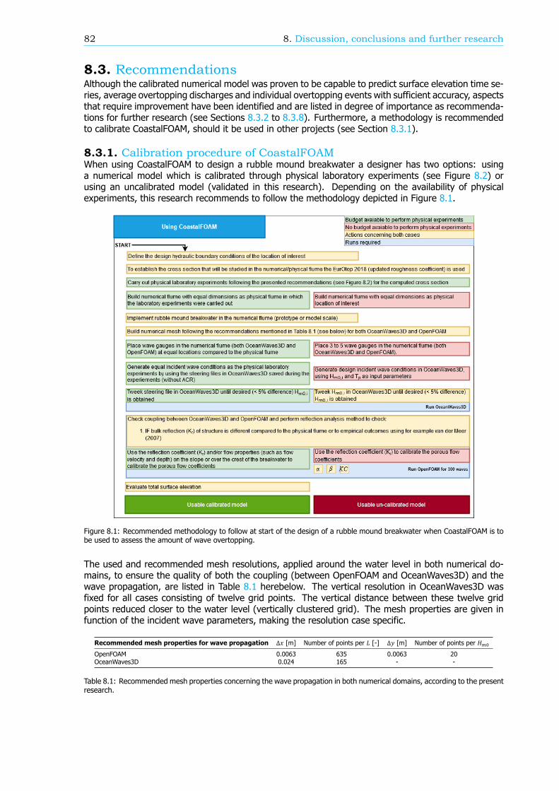
82 8. Discussion, conclusions and further research

8.3. RecommendationsAlthough the calibrated numerical model was proven to be capable to predict surface elevation time se-ries, average overtopping discharges and individual overtopping events with sufficient accuracy, aspectsthat require improvement have been identified and are listed in degree of importance as recommenda-tions for further research (see Sections 8.3.2 to 8.3.8). Furthermore, a methodology is recommendedto calibrate CoastalFOAM, should it be used in other projects (see Section 8.3.1).

8.3.1. Calibration procedure of CoastalFOAMWhen using CoastalFOAM to design a rubble mound breakwater a designer has two options: usinga numerical model which is calibrated through physical laboratory experiments (see Figure 8.2) orusing an uncalibrated model (validated in this research). Depending on the availability of physicalexperiments, this research recommends to follow the methodology depicted in Figure 8.1.

Figure 8.1: Recommended methodology to follow at start of the design of a rubble mound breakwater when CoastalFOAM is tobe used to assess the amount of wave overtopping.

The used and recommended mesh resolutions, applied around the water level in both numerical do-mains, to ensure the quality of both the coupling (between OpenFOAM and OceanWaves3D) and thewave propagation, are listed in Table 8.1 herebelow. The vertical resolution in OceanWaves3D wasfixed for all cases consisting of twelve grid points. The vertical distance between these twelve gridpoints reduced closer to the water level (vertically clustered grid). The mesh properties are given infunction of the incident wave parameters, making the resolution case specific.

Recommended mesh properties for wave propagation Δ𝑥 [m] Number of points per 𝐿 [-] Δ𝑦 [m] Number of points per 𝐻OpenFOAM 0.0063 635 0.0063 20OceanWaves3D 0.024 165 - -

Table 8.1: Recommended mesh properties concerning the wave propagation in both numerical domains, according to the presentresearch.

83

Figure 8.2: In the event that physical laboratory experiments are to be performed the present research recommends to carryout steps 1 to 7 and collect the best possible data to calibrate the numerical model.

Considering further improvement and extension of the numerical model:

8.3.2. OceanWaves3D and OpenFOAM couplingIn this research the coupling between OceanWaves3D and OpenFOAM for steep waves (extremes)was improved by increasing the resolution in propagating direction (x-axis). However, this solutionincreased computational time (approximately by a factor 2 on average over all cases). It is thereforerecommended to look at numerically more attractive solutions to improve the coupling.

8.3.3. Forces on protruding wave wallIn the present research the numerical model was set-up according to Jacobsen et al. (2018) as start-ing point. Jacobsen et al. (2018) used this set-up to validate: the numerical solution to avoid airentrapment (degree of openness of the wave wall) and the forces acting on a protruding wave wall.Nonetheless, discrepancies in the set-up were identified and tackled, and this resulted in a calibratedmodel. The calibrated model showed improved results when compared with measurements in termsof the cumulative overtopping curve. As a consequence, it is expected that the calibrated model willshow differences with the reported findings by Jacobsen et al. (2018) concerning the forces acting onthe protruding wave wall. It is thus recommended to use the calibrated model set-up and compare theoutcomes with the findings reported in Jacobsen et al. (2018) in order to show if the advised degreeof openness (3%) is still valid.

8.3.4. Bulk resistance structureAs shown by Losada et al. (2016) a wide set of dimensionless resistance coefficients (𝛼, 𝛽 and 𝐾𝐶)has been used numerically to recreate the porous flow and resulting bulk reflection coefficients of thebreakwater. First, it is recommended to use the presently selected set within another case study to see ifthe proposed coefficients are applicable to other situations. Second, as shown in this research, multiplesets of dimensionless coefficients can be used to correctly reconstruct the presence of the structure,defined by the reflection coefficient (𝐾 ). Consequently, the designer should adopt a different evaluationmethodology to select the set of porous flow coefficients, by accounting for additional evaluation criteria(for example the flow along the slope or over the crest of the breakwater), and see what the influenceis on the overtopping results.

8.3.5. Hydraulic boundary conditionsThe validation procedure considered the variation of wave height (𝐻 ), peak period (𝑇 ) and geometry(𝑅 , protruding and non-protruding). Nevertheless, the variation of the mean water level was discarded

84 8. Discussion, conclusions and further research

to reduce workload. However, the water level is an important hydraulic parameter when consideringwave overtopping, where 𝑞 is correlated to 𝑅 (Van der Meer et al., 2018). It is therefore recommendedto perform additional validation runs with varying water levels for which data is available, as shown inChapter 2.

8.3.6. Increased geometrical complexityThe model was validated for a conventional rubble mound breakwater with or without protruding wavewall. Yet, many other types of rubble mound breakwaters do exist, e.g. rubble mound breakwaterswith toe structure, berm or multiple protruding wave walls. It is thus recommended to test and validatethe proposed calibration methodology for rubble mound breakwaters for which no empirical method-ologies exist.

Considering the proposed NewWave methodologies:

8.3.7. Second-order wave generationThe first order wave generation introduced spurious waves which increased for increasing non-linearity.One possible solution is to use the second order wave generation by Schaffer (1995). It is recommendedto compare the overtopping results considering a NewWave profile generated with a first or secondorder wave generation. The comparison will show how big the influence of the spurious waves is onthe overtopping results when considering wave overtopping over rubble mound breakwaters, as similarto what has been done for sloping foreshores by Orszaghova et al. (2014).

8.3.8. Crest elevationOther methods do exist to obtain the crest height from the design wave height (instead of assuming𝜂 = 𝐻/2), which consider the water depth, deep water steepness and the slope of the foreshore toestimate the crest elevation using the cnoidal theory (Buhr Hansen, 1990). Another option is to runother type of numerical models (e.g. Mike 3 Wave FM model or SWASH) beforehand, to generate theincoming surface elevation time series (offshore to nearshore), giving an improved prediction of the𝜂 . % value at the toe of the breakwater. This 𝜂 . % value is recommended and can thus be used asinput for the proposed NewWave methodology.

References

W. Allsop, T. Bruce, J. M. Pearson, and J. Alderson. Violent wave overtopping at the coast, when arewe safe? Impact wave-forces View project Input to the Concrete Manual View project. Proceedingsof the International Conference on Coastal Management, pages 1–16, 2003. URL https://www.researchgate.net/publication/287547182.

P. Aminti and L. Franco. WAVE OVERTOPPING ON RUBBLE MOUND BREAKWATERS. 1988.

A. Antonini, R. Archetti, and A. Lamberti. Wave simulation for the design of an innovative quay wall:The case of Vlorë Harbour. Natural Hazards and Earth System Sciences, 17(1):127–142, 2017. ISSN16849981. doi: 10.5194/nhess-17-127-2017.

C. Arrighi, H. Oumeraci, and F. Castelli. Hydrodynamics of pedestrians’ instability in floodwaters.Hydrology and Earth System Sciences, 21(1):515–531, 2017. ISSN 16077938. doi: 10.5194/hess-21-515-2017.

J. A. Battjes and H. W. Groenendijk. Shallow foreshore wave height statistic. Proc. CoastalStructures, (January):29–35, 1999. URL http://repository.tudelft.nl/view/ir/uuid:fe03dda9-40d9-4046-87fb-459f01fcd3d3/.

E. Berberović, N. P. Van Hinsberg, S. Jakirlić, I. V. Roisman, and C. Tropea. Drop impact onto a liquidlayer of finite thickness: Dynamics of the cavity evolution. Physical Review E - Statistical, Nonlinear,and Soft Matter Physics, 79(3), 2009. ISSN 15393755. doi: 10.1103/PhysRevE.79.036306.

P. Besley. Wave overtopping of seawalls, design and assessment manual. R &D tech-nical report W178, (February):37, 1999. URL http://www.scribd.com/doc/7333031/-Over-Topping-Manual.

S. Boersen, O. Scholl, N. Jacobsen, and C. van der Lem. APPLYING A NUMERICAL WAVE FLUME TOPREDICT WAVE OVERTOPPING. In 38th IAHR World Congress, number 1, page 10, Panama City,2019.

M. Bozorgnia, J.-J. Lee, and F. Raichlen. Wave Structure Interaction: Role of Entrapped Air on WaveImpact and Uplift Forces. Coastal Engineering Proceedings, 1(32):57, 2012. ISSN 0589-087X. doi:10.9753/icce.v32.structures.57.

A. P. Bradbury, N. W. H. Allsop, and R. V. Stephens. Hydraulic Performance of Breakwater Crown Walls.(March):1–108, 1988.

T. Bruce, J. W. van der Meer, L. Franco, and J. M. Pearson. Overtopping performance of differentarmour units for rubble mound breakwaters. Coastal Engineering, 56(2):166–179, 2009. ISSN03783839. doi: 10.1016/j.coastaleng.2008.03.015. URL http://dx.doi.org/10.1016/j.coastaleng.2008.03.015.

J. Buhr Hansen. Periodic Waves in the Surf Zone: Analysis of Experimental Data. Coastal Engineering,14:19–41, 1990.

S. Caires and M. R. Van Gent. Wave height distribution in constant and finite depths. Proceedings ofthe Coastal Engineering Conference, 2012. ISSN 0589-087X. doi: 10.9753/icce.v33.waves.15.

M. Castellino, P. Sammarco, A. Romano, L. Martinelli, P. Ruol, L. Franco, and P. De Girolamo. Largeimpulsive forces on recurved parapets under non-breaking waves. A numerical study. Coastal Engi-neering, 136:1–15, 2018. ISSN 03783839. doi: 10.1016/j.coastaleng.2018.01.012.

85

86 References

N. Chini and P. K. Stansby. Extreme values of coastal wave overtopping accounting for climatechange and sea level rise. Coastal Engineering, 65:27–37, 2012. ISSN 03783839. doi: 10.1016/j.coastaleng.2012.02.009. URL http://dx.doi.org/10.1016/j.coastaleng.2012.02.009.

CIRIA, CUR, and CETMEF. Chapter 5 of The Rock Manual. Physical processes and design tools (2ndedition). C683, CIRIA, London, 2007a.

CIRIA, CUR, and CETMEF. Chapter 3 of The Rock Manual. Materials (2nd edition). C683, CIRIA, London,2007b.

G. Cuomo, K. i. Shimosako, and S. Takahashi. Wave-in-deck loads on coastal bridges and the role ofair. Coastal Engineering, 56(8):793–809, 2009. ISSN 03783839. doi: 10.1016/j.coastaleng.2009.01.005. URL http://dx.doi.org/10.1016/j.coastaleng.2009.01.005.

R. G. Dean and R. A. Dalrymple. Water Wave Mechanics for Engineers and Scientists. Advanced Serieson Ocean Engineering, Volume 2, 1991.

J. Dekker, S. Caires, and M. R. van Gent. Reflection of non-standard wave spectra by sloping structures.Proc. Coastal Structures, pages 760–770, 2007.

A. P. Engsig-Karup, H. B. Bingham, and O. Lindberg. An efficient flexible-order model for 3D nonlinearwater waves. Journal of Computational Physics, 228(6):2100–2118, 2009. ISSN 00219991. doi:10.1016/j.jcp.2008.11.028. URL http://dx.doi.org/10.1016/j.jcp.2008.11.028.

L. Franco, M. de Gerloni, and J. W. van der Meer. Wave overtopping on vertical and composite break-waters. Coastal Engineering, pages 1030–1045, 1994.

J. Geeraerts, P. Troch, J. De Rouck, H. Verhaeghe, and J. J. Bouma. Wave overtopping at coastalstructures: prediction tools and related hazard analysis. Journal of Cleaner Production, 15(16):1514–1521, 2007. ISSN 09596526. doi: 10.1016/j.jclepro.2006.07.050.

M. Hayatdavoodi, B. R. Seiffert, and R. C. Ertekin. Experiments and computations of solitary-waveforces on a coastal-bridge deck. Part II: Deck with girders. Coastal Engineering, 88(November 2017):210–228, 2014. ISSN 03783839. doi: 10.1016/j.coastaleng.2014.02.007.

P. Higuera, J. L. Lara, and I. J. Losada. Simulating coastal engineering processes with OpenFOAM®.Coastal Engineering, 71:119–134, 2013. ISSN 03783839. doi: 10.1016/j.coastaleng.2012.06.002. URL http://dx.doi.org/10.1016/j.coastaleng.2012.06.002.

P. Higuera, J. L. Lara, and I. J. Losada. Three-dimensional interaction of waves and porous coastalstructures using OpenFOAM®. Part II: Application. Coastal Engineering, 83:259–270, 2014a. ISSN03783839. doi: 10.1016/j.coastaleng.2013.09.002. URL http://dx.doi.org/10.1016/j.coastaleng.2013.09.002.

P. Higuera, J. L. Lara, and I. J. Losada. Three-dimensional interaction of waves and porous coastalstructures using OpenFOAM®. Part I: Formulation and validation. Coastal Engineering, 83:243–258,2014b. ISSN 03783839. doi: 10.1016/j.coastaleng.2013.08.010. URL http://dx.doi.org/10.1016/j.coastaleng.2013.08.010.

B. Hofland, I. Wenneker, and P. V. Steeg. Short Test Durations for Wave Overtopping Experiments.Conference Paper, (SEPTEMBER):1–10, 2014.

T. J. Hsu, T. Sakakiyama, and P. L. Liu. A numerical model for wave motions and turbulence flows infront of a composite breakwater. Coastal Engineering, 46(1):25–50, 2002. ISSN 03783839. doi:10.1016/S0378-3839(02)00045-5.

N. G. Jacobsen and J. Fredsoe. Formation and development of a breaker bar under regular waves. Part2: Sediment transport and morphology. Coastal Engineering, 88:55–68, 2014. ISSN 03783839. doi:10.1016/j.coastaleng.2014.01.015. URL http://dx.doi.org/10.1016/j.coastaleng.2014.01.015.

87

N. G. Jacobsen, D. R. Fuhrman, and J. Fredsøe. A wave generation toolbox for the open-source CFDlibrary: OpenFoam®. International Journal for Numerical Methods in Fluids, 70(9):1073–1088, 2012.ISSN 02712091. doi: 10.1002/fld.2726.

N. G. Jacobsen, M. R. van Gent, and G. Wolters. Numerical analysis of the interaction of irregular waveswith two dimensional permeable coastal structures. Coastal Engineering, 2015. ISSN 03783839. doi:10.1016/j.coastaleng.2015.05.004.

N. G. Jacobsen, M. R. van Gent, and J. Fredsøe. Numerical modelling of the erosion and deposi-tion of sand inside a filter layer. Coastal Engineering, 120(September 2016):47–63, 2017. ISSN03783839. doi: 10.1016/j.coastaleng.2016.09.003. URL http://dx.doi.org/10.1016/j.coastaleng.2016.09.003.

N. G. Jacobsen, M. R. van Gent, A. Capel, and M. Borsboom. Numerical prediction of integrated waveloads on crest walls on top of rubble mound structures. Coastal Engineering, 142(April 2017):110–124, 2018. ISSN 03783839. doi: 10.1016/j.coastaleng.2018.10.004. URL https://doi.org/10.1016/j.coastaleng.2018.10.004.

B. Jensen, N. G. Jacobsen, and E. D. Christensen. Investigations on the porous media equationsand resistance coefficients for coastal structures. Coastal Engineering, 84:56–72, 2014. ISSN03783839. doi: 10.1016/j.coastaleng.2013.11.004. URL http://dx.doi.org/10.1016/j.coastaleng.2013.11.004.

P. Jonathan and P. H. Taylor. Irregular, non-linear waves in a spread sea. Proceedings of the InternationalConference on Offshore Mechanics and Arctic Engineering - OMAE, 1(Part A):9–16, 1995. ISSN1528896X. doi: 10.1115/1.2829043.

Kansai Airport. FY2018 Consolidated Finanacial Resulst. Technical report, Kansai Region, 2019.

N. Karagiannis, T. Karambas, and C. Koutitas. Wave overtopping numerical simulation using OpenFoam.E-Proceeding of the 36th IAHR world congress, 2(2012):1–12, 2015.

J. L. Lara, M. del Jesus, and I. J. Losada. Three-dimensional interaction of waves and porous coastalstructures. Coastal Engineering, 64:26–46, 2012a. ISSN 03783839. doi: 10.1016/j.coastaleng.2012.01.009. URL http://dx.doi.org/10.1016/j.coastaleng.2012.01.009.

J. L. Lara, M. del Jesus, and I. J. Losada. Three-dimensional interaction of waves and porous coastalstructures. Coastal Engineering, 64:26–46, 2012b. ISSN 03783839. doi: 10.1016/j.coastaleng.2012.01.009. URL http://dx.doi.org/10.1016/j.coastaleng.2012.01.008.

P. Lin and S. A. Karunarathna. Numerical Study of Solitary Wave Interaction with Porous Breakwaters.Journal of Waterway, Port, Coastal, and Ocean Engineering, 133(5):352–363, 2007. ISSN 0733-950X.doi: 10.1061/(asce)0733-950x(2007)133:5(352).

G. Lindgren. Some Properties of a Normal Process Near a Local Maximum. the Annals of MathematicalStatistics. Annals of Mathematical Statistics, 41(6):1870–1883, 1970.

I. J. Losada, J. L. Lara, R. Guanche, and J. M. Gonzalez-Ondina. Numerical analysis of wave overtoppingof rubble mound breakwaters. Coastal Engineering, 55(1):47–62, 2008. ISSN 03783839. doi:10.1016/j.coastaleng.2007.06.003.

I. J. Losada, J. L. Lara, and M. del Jesus. Modeling the Interaction of Water Waves with Porous CoastalStructures. Journal of Waterway, Port, Coastal, and Ocean Engineering, 142(6):03116003, 2016.ISSN 0733-950X. doi: 10.1061/(asce)ww.1943-5460.0000361.

J. Molines and J. R. Medina. Calibration of overtopping roughness factors for concrete armor units innon-breaking conditions using the CLASH database. Coastal Engineering, 96:62–70, 2015. ISSN03783839. doi: 10.1016/j.coastaleng.2014.11.008.

J. Molines and J. R. Medina. Explicit Wave-Overtopping Formula for Mound Breakwaters with CrownWalls Using CLASH Neural Network–Derived Data. Journal of Waterway, Port, Coastal, and OceanEngineering, 142(3):04015024, 2016. ISSN 0733-950X. doi: 10.1061/(asce)ww.1943-5460.0000322.

88 References

J. Orszaghova, P. H. Taylor, A. G. Borthwick, and A. C. Raby. Importance of second-order wave gener-ation for focused wave group run-up and overtopping. Coastal Engineering, 94(1959):63–79, 2014.ISSN 03783839. doi: 10.1016/j.coastaleng.2014.08.007.

B. T. Paulsen, H. B. Bingham, and H. Bredmose. Efficient computations of wave loads on offshorestructures. (August):152, 2013.

J. Pearson, T. Bruce, L. Franco, J. W. van der Meer, M. Falzacappa, and R. Molino. Roughness factor.Technical report, Work package 4.4, D24 Report on additional tests, Part B, CLASH reportEVK3-CT-2001-00058, 2004.

Port of Rotterdam. Facts & Figures about the port, 2018. URL https://www.portofrotterdam.com/sites/default/files/feiten-en-cijfers-haven-rotterdam.pdf?token=PBcH9rLs.

T. Pullen, H. R. Wallingford, N. W. H. Allsop, T. Bruce, and C. Mitchel. The EurOtop Team Authors:Steering group: Funding bodies. (August), 2007.

A. Romano, G. Bellotti, R. Briganti, and L. Franco. Uncertainties in the physical modelling of the waveovertopping over a rubble mound breakwater: The role of the seeding number and of the testduration. Coastal Engineering, 103:15–21, 2015. ISSN 03783839. doi: 10.1016/j.coastaleng.2015.05.005.

H. A. Schaffer. Pergamon SECOND-ORDER WAVEMAKER THEORY FOR IRREGULAR WAVES. OceanEngineering, 23(1):47–88, 1995.

J. G. Schierirck and H. J. Verhagen. Introduction to bed, bank, shore protection. Delft Academic Press,2016.

B. R. Seiffert, M. Hayatdavoodi, and R. C. Ertekin. Experiments and computations of solitary-waveforces on a coastal-bridge deck. Part I: Flat Plate. Coastal Engineering, 88(November 2017):194–209, 2014. ISSN 03783839. doi: 10.1016/j.coastaleng.2014.01.005.

B. R. Seiffert, R. C. Ertekin, and I. N. Robertson. Wave loads on a coastal bridge deck and the role ofentrapped air. Applied Ocean Research, 2015. ISSN 01411187. doi: 10.1016/j.apor.2015.07.010.

TAW. Technisch rapport golfoploop en golfoverslag bij dijken/Wave run-up and waveovertopping atdikes, 2002.

P. S. Tromans, A. R. Anatruk, and P. Hagemeijer. New model for the kinematics of large ocean wavesapplication as a design wave. Proceedings of the First International Offshore and Polar EngineeringConference, August 11, 1991 - August 16, Ill(August):64–71, 1991.

J. Van den Bos, H. Verhagen, and C. Kuiper. Numerical modelling of wave reflection and transmissionin vertical porous structures. page 16. ASCE - COPRI, 2015.

J. van der Meer and T. Bruce. New Physical Insights and Design Formulas on Wave Overtopping atSloping and Vertical Structures. Journal of Waterway, Port, Coastal, and Ocean Engineering, 140(6):04014025, 2013. ISSN 0733-950X. doi: 10.1061/(asce)ww.1943-5460.0000221.

J. Van der Meer, N. Allsop, D. R. Bruce, T., A. J., Kortenhaus, T. Pullen, H. Schüttrumpf, P. Troch, andB. Zanuttigh. EurOtop, 2018. Manual on wave overtopping of sea defences and related structures.An overtopping manual largely based on European research, but for worldwide application. page320, 2018. URL www.overtopping-manual.com.

M. R. van Gent. Wave interaction with permeable coastal structures. International Journal of RockMechanics and Mining Sciences & Geomechanics Abstracts, 33(6):A277, 1995. ISSN 01489062. doi:10.1016/0148-9062(96)81968-1.

M. R. van Gent. Physical model investigations on coastal structures with shallow foreshores; 2D modeltest with single and double-peaked wave energy spectra, 1999.

89

M. R. van Gent and G. Wolters. Granular slopes with open filters under wave loading. Coastal Engi-neering, 104:135–150, 2015. ISSN 03783839. doi: 10.1016/j.coastaleng.2015.06.004.

M. R. van Gent, H. F. van den Boogaard, B. Pozueta, and J. R. Medina. Neural network modelling ofwave overtopping at coastal structures. Coastal Engineering, 54(8):586–593, 2007. ISSN 03783839.doi: 10.1016/j.coastaleng.2006.12.001.

M. R. van Gent, N. G. Jacobsen, and G. Wolters. Modelling of open filters under wave loading.(September):2–11, 2017. URL https://www.researchgate.net/publication/319877988.

J. Van Os, S. Caires, and M. Van Gent. Guidelines for metocean data analysis. Proceedings of theInternational Offshore and Polar Engineering Conference, (January 2011):290–297, 2011. ISSN10986189.

D. Vanneste and P. Troch. 2D numerical simulation of large-scale physical model tests of wave interac-tion with a rubble-mound breakwater. Coastal Engineering, 103:22–41, 2015. ISSN 03783839. doi:10.1016/j.coastaleng.2015.05.008. URL http://dx.doi.org/10.1016/j.coastaleng.2015.05.008.

H. Verhagen and J. Van den Bos. Breakwater design: Lecture notes CIE5308. (Draft), 2018.

H. G. Weller, G. Tabor, H. Jasak, and C. Fureby. A tensorial approach to computational continuum me-chanics using object-oriented techniques. Computers in Physics, 12(6):620, 1998. ISSN 08941866.doi: 10.1063/1.168744. URL http://scitation.aip.org/content/aip/journal/cip/12/6/10.1063/1.168744.

C. N. Whittaker, A. C. Raby, C. J. Fitzgerald, and P. H. Taylor. The average shape of large wavesin the coastal zone. Coastal Engineering, 114:253–264, 2016. ISSN 03783839. doi: 10.1016/j.coastaleng.2016.04.009. URL http://dx.doi.org/10.1016/j.coastaleng.2016.04.009.

C. N. Whittaker, C. J. Fitzgerald, A. C. Raby, P. H. Taylor, J. Orszaghova, and A. G. Borthwick. Op-timisation of focused wave group runup on a plane beach. Coastal Engineering, 121(November2016):44–55, 2017. ISSN 03783839. doi: 10.1016/j.coastaleng.2016.12.001. URL http://dx.doi.org/10.1016/j.coastaleng.2016.12.001.

C. N. Whittaker, C. J. Fitzgerald, A. C. Raby, P. H. Taylor, and A. G. Borthwick. Extreme coastal responsesusing focused wave groups: Overtopping and horizontal forces exerted on an inclined seawall.Coastal Engineering, 140(March):292–305, 2018. ISSN 03783839. doi: 10.1016/j.coastaleng.2018.08.004. URL https://doi.org/10.1016/j.coastaleng.2018.08.004.

J. Zelt and J. E. Skjelbreia. Estimating Incident and Reflected Wave Fields Using an Arbitrary Number ofWave Gauges. Coastal Engineering, pages 777–789, 1992. doi: 10.1061/9780872629332.058.

AAppendix A

Case 𝐻 [m] 𝑇 [s] 𝑇 , [s] ℎ [m] 𝜉 , [-] 𝐾 [-] Ursell [-] 𝑞 [l/s/m] 𝑞 [l/s/m]A1W1T101 0.08 1.82 1.73 0.80 3.77 0.31 3.51 0.004 0.78A1W1T102 0.10 2.12 1.98 0.80 3.84 0.33 7.59 0.037 8.03A1W1T103 0.12 2.26 2.22 0.80 3.96 0.36 14.28 0.181 37.36A1W1T104 0.08 1.45 1.35 0.80 2.97 0.23 1.30 0.001 0.26A1W1T105 0.10 1.63 1.51 0.80 2.94 0.25 2.57 0.027 5.88A1W1T106 0.12 1.72 1.66 0.80 2.94 0.28 4.50 0.149 31.34A1W1T107 0.08 1.14 1.12 0.80 2.50 0.19 0.59 0.000 0.00A1W1T108 0.10 1.29 1.25 0.80 2.45 0.19 1.16 0.013 2.89A1W1T109 0.12 1.37 1.37 0.80 2.46 0.20 2.06 0.084 18.13A1W1T201 0.10 2.03 1.99 0.75 3.86 0.33 9.37 0.002 0.36A1W1T202 0.12 2.26 2.25 0.75 3.98 0.37 18.48 0.014 2.91A1W1T203 0.14 2.51 2.47 0.75 4.16 0.40 29.32 0.044 9.59A1W1T204 0.10 1.63 1.51 0.75 2.94 0.25 3.15 0.001 0.30A1W1T205 0.12 1.76 1.67 0.75 2.96 0.28 5.65 0.025 5.37A1W1T206 0.15 1.94 1.87 0.75 3.06 0.29 10.41 0.078 16.55A1W1T207 0.10 1.24 1.25 0.75 2.47 0.20 1.39 0.002 0.41A1W1T208 0.12 1.37 1.39 0.75 2.48 0.21 2.60 0.012 2.60A1W1T209 0.14 1.46 1.50 0.75 2.48 0.22 4.17 0.052 11.32A1W1T301 0.12 2.26 2.29 0.70 4.06 0.36 24.38 0.000 0.00A1W1T302 0.14 2.51 2.54 0.70 4.21 0.41 42.13 0.011 2.28A1W1T303 0.16 2.61 2.79 0.70 4.31 0.45 69.78 0.072 15.48A1W1T304 0.12 1.72 1.70 0.70 3.01 0.27 7.29 0.001 0.16A1W1T305 0.15 1.93 1.90 0.70 3.12 0.30 13.59 0.012 2.48A1W1T306 0.17 2.00 2.11 0.70 3.24 0.32 23.51 0.049 10.49A1W1T307 0.12 1.37 1.39 0.70 2.49 0.21 3.20 0.000 0.00A1W1T308 0.14 1.46 1.52 0.70 2.51 0.23 5.43 0.010 2.25A1W1T309 0.16 1.60 1.64 0.70 2.55 0.25 8.27 0.033 7.13A3W1T101 0.08 1.82 1.74 0.80 3.76 0.31 3.61 0.037 7.89A3W1T102 0.11 2.12 1.99 0.80 3.84 0.34 7.93 0.256 54.81A3W1T103 0.13 2.26 2.23 0.80 3.94 0.36 14.78 0.731 155.82A3W1T104 0.08 1.45 1.36 0.80 2.96 0.23 1.35 0.014 3.06A3W1T105 0.11 1.63 1.52 0.80 2.92 0.26 2.64 0.138 29.40A3W1T106 0.13 1.72 1.68 0.80 2.95 0.28 4.79 0.542 113.10A3W1T107 0.08 1.14 1.13 0.80 2.51 0.20 0.62 0.005 1.09A3W1T108 0.10 1.29 1.26 0.80 2.46 0.20 1.23 0.066 14.28A3W1T109 0.12 1.35 1.39 0.80 2.47 0.21 2.17 0.301 64.22A3W1T201 0.11 2.03 2.00 0.75 3.84 0.33 9.79 0.022 4.73A3W1T202 0.12 2.26 2.25 0.75 3.98 0.36 18.28 0.088 18.95A3W1T203 0.14 2.51 2.48 0.75 4.17 0.39 30.38 0.267 56.74A3W1T204 0.10 1.63 1.52 0.75 2.93 0.25 3.22 0.010 2.11A3W1T205 0.13 1.76 1.68 0.75 2.96 0.28 5.80 0.088 18.43A3W1T206 0.15 1.94 1.88 0.75 3.05 0.29 10.76 0.358 74.68A3W1T207 0.10 1.29 1.25 0.75 2.46 0.19 1.45 0.010 2.11A3W1T208 0.12 1.37 1.39 0.75 2.47 0.20 2.67 0.056 11.93A3W1T209 0.14 1.46 1.51 0.75 2.48 0.22 4.31 0.195 42.18A3W1T301 0.13 2.26 2.30 0.70 4.02 0.38 25.34 0.010 2.04A3W1T302 0.15 2.51 2.59 0.70 4.18 0.41 47.52 0.084 17.91A3W1T303 0.17 2.61 2.81 0.70 4.29 0.46 73.66 0.249 52.10A3W1T304 0.13 1.72 1.70 0.70 2.98 0.29 7.59 0.016 3.26A3W1T305 0.15 1.93 1.92 0.70 3.10 0.31 14.29 0.053 11.33A3W1T306 0.17 2.00 2.13 0.70 3.22 0.33 24.91 0.186 39.08A3W1T307 0.12 1.37 1.39 0.70 2.47 0.22 3.32 0.009 1.92A3W1T308 0.15 1.46 1.53 0.70 2.50 0.25 5.71 0.032 6.82A3W1T309 0.16 1.60 1.65 0.70 2.54 0.27 8.65 0.110 23.69

Table A.1: Hydraulic boundary conditions for all 54 experimental cases. First half containing cases with protruding wave wall,defined by the A1 code. The bottom half containing the cases without protruding wave wall element with code A3. The waterdepth is described by the T-code, where cases containing T1 are for a water depths of 0.80 m, T2 for 0.75 m and T3 for 0.70 m.

91

BAppendix B

B.1. Time lagA time step error between measured and modelled incoming surface elevations, increasing over time,is captured. Two possibilities are discussed next:

∘ Numerical diffusion: errors (between modelled and measured) due to the introduction of simplifi-cations and assumptions into the numerical framework compared to the real world. The numericalmodel is not an exact representation of the experimental flume. However, for each modelled wavetraveling towards the structure, the error induced due to numerical diffusion would be the same.Therefore, the induced time lag would be close to constant at a selected wave gauge. However,the time step error increases in time and not over the distance covered by the travelling waves.This rules out numerical diffusion as cause.

∘ The time steps for which the steering velocities are written out are coarse (0.04 s), two decimals.Therefore, small differences between recorded time steps for which the velocities of the paddleare written off in the physical model and the steering signal used to reconstruct the same waveclimate, induce errors over 1800 simulated seconds (1000 waves).

This is solved by applying the following correction (see Equation B.1), to each time step for which thevelocity is written out within the original steering file.

𝑇 = 0 ∶ Δ𝑇 /𝑁 ∶ Δ𝑇 (B.1)

Where Δ𝑇 has been established by applying the ”finddelay” function in MATLAB at the end of thesurface elevation time series. Now modelled and measured signals can be compared by means ofRMSE (Root mean squared error) and PCC (Pearson correlation coefficient) values. Before, due to timeshifts, the signals could not be compared with the aforementioned statistical parameters.

B.2. Amplification steering paddleThe uncoupled incoming modelled surface elevation spectrum in OceanWaves3D (A2 steering file)and the incoming measured wave signal spectrum, are shown Figure B.1. Table B.1 describes therelation between both signal by means of spectral and statistical parameters. It can be inferred thatthe base OceanWaves3D steering file generates under dimensioned (-8%) incoming wave conditions(in terms of 𝐻 ) when comparing to the measured incoming wave conditions. However, when theoriginal steering files (Base = RAW) are compared with the provided steering files within the JIP,amplification factors can be inferred, used in order to achieve improved comparisons between modelledand measured wave incident conditions. The applied technique uses a constant factor over all timesteps. In the present research, a frequency based amplification is preferred, explained in intermezzo -Amplification.

93

94 Appendix B

Figure B.1: Incoming modelled and measured spectra at wave gauge closest to structure (5), x = 40.10 m. Showing that theamplification performed in this research performs better in terms of spectral wave height comparison with measurements.

Intermezzo - Amplification

In order to achieve an improved comparison between incoming modelled and measured surfaceelevations, a frequency based amplification is performed. This required multiple chronologicalsteps:

1. A spectral comparison is made between the base (provided raw steering file) incomingsurface elevation modelled within OCW3D (with the non-amplified steering files) and mea-sured incoming surface elevation (achieved after applying the reflection analysis method).

2. Both signals are interpolated to equal time steps, transformed to spectra and divided byeach other, giving an amplification factor which varies over the frequency band.

3. The velocity spectrum is obtained from the provided steering files (velocities per time step,interpolated to the equal time steps as the previous two data sets).

4. The square root of the frequency based amplification factor is multiplied with the veloc-ity spectrum, amplifying regions were discrepancies are encountered between modelledand measured signals. Amplifying the velocity spectrum in a range of interest results inamplifications in equal frequency ranges within the wave spectrum.

5. An inverse Fourier transform is executed to the amplified velocity spectrum in order toobtain the amplified steering file, used again as input in OCW3D, resulting in an amplifiedincoming surface elevation (OCW3D - Amplified = A3).

This process can be done iteratively in order to obtain the optimal match in terms of𝐻 betweenthe OCW3D and measured incoming wave signal. However, a second iteration step does notimprove RMSE and PCC values and therefore the first iteration step is sufficient. Around 500waves were used to compare the modelled wave conditions with measurements.

According to Table B.1 the amplification applied by Jacobsen et al. (2018) (Jacobsen = B1) showedimproved results, compared to the base (Base = RAW) case provided by Deltares, in terms of RMSEand PCC. However, RMSE and PCC values are sensitive for time shifts, which were applied previously to

95

improve the comparability between modelled and measured surface elevations. Therefore the spectralwave height is given more importance as evaluation factor. In that case, the amplification executed inthis research (A3) achieved the best result.

Case RMSE [m] PCC [%] Hm0 [%]OCW3D - RAW 0.0121 92.5 - 8.0%OCW3D - B1 0.0115 93.3 - 3.7%OCW3D - A3 0.0122 92.6 + 0.1%

Table B.1: Statistical and spectral parameters describing the relation between the various OCW3D configurations.

B.3. OceanWaves3D couplingComparing the OceanWaves3D (uncoupled) modelled incoming wave climate, detached from Open-FOAM, with the OceanWaves3D (coupled) modelled incoming wave climate extracted from an Open-FOAM run, gives Figure B.2. It can be concluded (see Figure B.2), that under the current conditions(A3) the numerical model is not capable to reproduce extreme waves accurately (high steepness).Upon coupling, 9.6% of the incoming wave condition (𝐻 ) is lost.

Figure B.2: Incident surface elevation captured at wave gauge closest to structure (No. 5), x = 40.10 m, showing the thediscrepancies in modelling the incident surface elevations (extreme waves) when OceanWaves3D is coupled to OpenFOAM.

The aforementioned phenomenon is caused by the coupling between OpenFOAM and OceanWaves3D,done by Paulsen et al. (2013). To solve the problem, the resolution in the propagation direction of theincoming waves (x-direction) needs to be increased, within OceanWaves3D domain. Instead of having85 grid points (which is much higher as the horizontal 10 grid points per leading wave length suggestedby Paulsen et al. (2013)) per leading wave length (𝑁 ) the number of grid points was doubled to 170.Various other set-ups have been tested, varying: time steps, Courant numbers and y-resolution, how-ever, without any success. Therefore, all x-directed resolutions of the provided OceanWaves3D.inputfiles were increased, ensuring good quality upon coupling. Applying the presented solution gives sig-nificant improvements in terms of spectral wave heights 𝐻 , losing 2.5%, (see Figure B.3).

Figure B.3: Incident surface elevation captured at wave gauge closest to structure (No. 5), x = 40.10 m, showing the improve-ment in coupling when adopting the proposed solution.

96 Appendix B

The reduction in 𝐻 can be further reduced by increasing the resolution, however, the computationaltime it would require is not worth the improvement in accuracy it would yield.

B.4. Reflection structureThe reflection of the structure is too high (𝐾 , = 0.34) compared to measurements (𝐾 , = 0.28).The bulk reflection of the rubble mound breakwater depends on various parameters, e.g. Irribarrennumber, the angle of the slope and the porous flow properties. As the first two factors can not bealtered, a closer look is given to the parametrisation by van Gent (1995) to describe the porous flowthrough the various layers of which the breakwater consists. In the upcoming sections the 𝑛 (porosity),𝛼, 𝛽 and 𝐾𝐶 coefficients are discussed.

PorosityIncreasing of the porosity lowers both resistance coefficients (𝑎 and 𝑏), reducing the resistance theincoming flow experiences and therefore reduces the reflection coefficient. The porosity of all layersin the numerical model has been set at 0.40, however, this was done without measuring it duringthe physical laboratory experiments. The Rock Manual 2007 (CIRIA et al., 2007b) suggests to useformulas (see Equations B.2 and B.3) to predict the average porosity for different gradings and shapecharacteristics. The Equation applies to all bulk-placed granular materials (core, filter and armour).The procedure was briefly discussed in Chapter 5. Here the methodology is elaborated. A procedure,estimating the porosity based on the grain size distribution parameters, such as the uniformity indexof the Rosin-Rammler (Ros-Ram) curve based on the grain diameter, 𝑛 .

𝑛 = 190 ⋅ (𝑒 ) ⋅ arctan(0.645 ⋅ 𝑛 ) ⋅ 180𝜋 (B.2)

𝑛 = 𝑒1 + 𝑒 (B.3)

Where, 𝑒 is the void ratio equal to the volume of voids divided by the volume of solids, 𝑒 the voidratio associated to the single-size particles of different shapes and 𝑛 the bulk porosity of the granularmaterial. For typically mechanical crushed the single-size void ratio (𝑒 ) ranges between 0.92-0.96and is taken as 0.94 here. In order to find the uniformity index describing the shape of the Ros-Ramcurve, the gradings of the granular materials are needed. The following gradings, for the differentlayers, were reported by Deltares and are listed in Table B.2. The grading curves are shown below.The Ros-Ram equation describes the typical shape of the mass/size grading curves and will be usedhere to estimate the bulk porosity of the granular materials.

Type Laboratory scale Prototype scale

Layer 𝐷𝑛 [mm] 𝐷𝑛 [mm] 𝐷𝑛 [mm] 𝐷𝑛 [mm] 𝐷𝑛 [mm] 𝐷𝑛 [mm] 𝑀 [kg] 𝑀 [kg] 𝑀 [kg]

Armour 20.6 32.1 52.4 741.6 1155.6 1886.4 1080.8 4089.5 17788.8Filter 11.5 16.5 23.8 414.0 594.0 856.8 188.0 555.4 1666.8Core 3.9 6.3 9.0 140.4 226.8 324 7.3 30.9 90.1

Table B.2: Grading parameters for different subdivisions of the rubble mound breakwater, on laboratory and prototype scale.

According to the Rock Manual 2007 guidelines the mass uniformity index (𝑛 ) can be determinedgiven any two fixed points on Ros-Ram curve (see Equations B.4-B.8). In practice, the nominal lowerlimit mass of a grading (𝑁𝐿𝐿) with the maximum allowable passing fraction 𝑦 , and similarly thenominal upper limit mass of a grading (𝑁𝑈𝐿) with the the maximum allowable passing fraction 𝑦 ,are set as two fixed points on the Ros-Ram curve. Combining both equations solves for the the massuniformity index, based on the pre-determined fractions of passing.

𝑦 = 1 − exp ⋅ (ln (12) ⋅𝑀𝑀 ) ≅ 1 − exp ⋅ (−0.693 ⋅

𝑀𝑀 ) (B.4)

the inverse:

97

𝑀 = 𝑀 ⋅ (ln(1 − 𝑦)ln ( )

)

/

≅ 𝑀 ⋅ (− ln(1 − 𝑦)0.693 )/

(B.5)

two fixed points:

𝑀 = 𝑁𝑁𝐿 ⋅ ( ln(1 − 𝑦 )−0.693 )

/(B.6)

𝑀 = 𝑁𝑈𝐿 ⋅ ( ln(1 − 𝑦 )−0.693 )

/(B.7)

reworked:

𝑛 =log ( ( )

( ))

log ( )(B.8)

Where, 𝑦 is the fraction passing value depending on the grading type (EN 13383 standard grading) ofthe granular material, 𝑀 is the mass of the granular particles corresponding to the fraction of passingand 𝑛 the mass uniformity index which is a measure for the steepness of the grading curve. In orderto find the EN 13383 standard gradings of the materials used during the experiments, the prototyperock masses were computed (𝜌 = 2650 kg/m , scale factor 36x) and are listed in Table B.2. Thecoefficient relating the nominal diameter (𝐷 ) with the diameter (𝐷) is taken as 0.84. The EN 13383standard grading table listed in Bed Bank and Shore protection (Schierirck and Verhagen, 2016) showsthat the gradings can be classified as heavy (armour), heavy (filter) and light (core). According tothe Rock Manual 2007 the fraction of passing (𝑦 and 𝑦 ) in cases of light-heavy gradings canbe chosen as 6% and 90% respectively. From the attached grading curves provided by Deltares (seeFigures B.4, B.5 and B.6), the 𝑀 % and 𝑀 % can be estimated which are used to re-evaluate 𝑛 .This resulted in the following 𝑛 values, 1.29 for the armour layer, 1.66 for the filter layer and1.47 for the core. Finally, the average bulk porosity of the granular materials can be estimated, usingEquations B.2 and B.3, where 𝑛 = 3 ⋅𝑛 , giving:

∘ 𝑛 = 0.416

∘ 𝑛 = 0.432

∘ 𝑛 = 0.425

Plugging in the re-evaluated porosities and 𝐷 , following the guidelines mentioned in the Rock Manual2007, the reflection coefficient 𝐾 , remains 0.34. The adaptations did not reduce the reflectionsufficiently and therefore additional changes are needed to lower the bulk reflection.

98 Appendix B

Figure B.4: Measured sieving curve of the armour layer in the physical flume.

Figure B.5: Measured sieving curve of the filter layer in the physical flume.

Figure B.6: Measured sieving curve of the core in the physical flume. Four different batches were used to construct the core ofthe breakwater in the physical flume. All four sieve curves are plotted against each other.

99

𝛼, 𝛽 and 𝐾𝐶From all the considered dimensionless porous flow coefficients sets by Losada et al. (2016) the tech-nique proposed by Jensen et al. (2014) is investigated here. Jensen et al. (2014) extended the researchby comparing experimental data sets with numerical model outcomes (using OpenFoam) for differentflow regimes (based on the porous Reynolds 𝑅𝑒 number) and ranges of dimensionless coefficients (𝛼and 𝛽). Four different flow regimes were characterised, the Darcy flow regime (laminar) 1 < 𝑅𝑒 < 10,the Forcheimer flow regime 10 < 𝑅𝑒 < 150, the transitional flow regime 150 < 𝑅𝑒 < 300 and the fullyturbulent flow regime 300 < 𝑅𝑒 . The regimes were determined based on the porous Reynolds numberand reconstructed with different dam break configurations. Three experimental laboratory test wereset up to represent each type of flow regime (except the laminar flow regime), which the numericalmodel tried to mimic by running several simulations with different dimensionless coefficients (𝛼 and𝛽). From this, three graphs were derived (see Figures B.7a, B.7b and B.7c). Each graph displays theerrors introduced by the numerical model when comparing modelled with measured surface elevationsrepresenting the dam break flow, for different combinations of coefficients. As the recommended coef-ficients according to van Gent (1995) produced a 𝐾 , which is too high, the ranges which introducedacceptable errors reported by Jensen et al. (2014) are selected and studied next. However, first thetype of flow regime needs to be determined. The porous Reynolds number is calculated using EquationB.9.

𝑅𝑒 =⟨�̄�⟩ ⋅ 𝐷𝑛 ⋅ 𝜈 (B.9)

Where, ⟨�̄�⟩ is the flow velocity averaged per time step and over each control volume (representing themost probable occurring flow regime in each cell) and 𝜈 the kinematic viscosity which at 18∘ is equalto 1.053e-06 m /s. Evaluating the type of flow is an iterative process (as the flow velocity will changefor different porosities and dimensionless resistance coefficients), however, here the reference case istaken as first estimate. The 𝑅𝑒 values will vary per cell, from which contour lines describing the flowtype over the breakwater can be derived. Instead of looking at the variation over all cells, the averageis taken over all cells contained within each layer type. The following flow regimes are found:

∘ 𝑅𝑒 , = 4468.1 - fully turbulent flow regime

∘ 𝑅𝑒 , = 1050.0 - fully turbulent flow regime

∘ 𝑅𝑒 , = 57.6 - Forcheimer flow regime

All flow regimes lie within the region where a non-linear relation between the resistance and the flowrate appears. For the armour and filter layer the third graph (turbulent flow; see Figure B.7c) canbe used. Jensen et al. (2014) noticed that in case of turbulent flow the dependency on the turbulentcoefficient 𝛽 is high, which was also noticed by Losada et al. (2008). In case of the core the firstgraph, Figure B.7a, must be used for the selection of a set of dimensionless coefficients. From all theforegoing the following sets are tested in the numerical model (1) 𝛼 = 500, 𝛽 = 2 for each layer and(2) 𝛼 = 0.001, 𝛽 = 1.1 for armour and filter and 𝛼 = 250, 𝛽 = 0.75 for the core.

(a) = 62. (b) = 325. (c) = 2750.

Figure B.7: The dimensionless resistance coefficient plotted against the dimensionless resistance coefficients. Contoursof the error between simulated and experimental surface elevations, using a set of dimensionless resistance coefficients, fordifferent flow regimes (characterised by the porous Reynolds number ( )).

CAppendix C

C.1. Spectrum fitThe following figures show the spectrum fit applied to the measured incident wave conditions for eachstudied incoming wave condition (T201-T209), except the ones already reported in Chapter 6.

(a) T201. (b) T202. (c) T203.

(d) T204. (e) T206. (f) T207.

(g) T208. (h) T209.

Figure C.1: Showing two possible spectrum fits applied to the incoming wave spectrum. Where the JONSWAP ( = 3.3) showeda good comparison with the measured incoming spectrum. Grey lines showing the threshold cut-off limits and . CasesT201 to T209 without T205.

101

102 C. Appendix C

C.2. Composite Weibull distributionThe following figures show the Composite Weibull distribution for each studied incident wave condition(T201-T209), except the ones already reported in Chapter 6, compared with the incident measuredwave heights. The latter were obtained by applying a reflection analysis combined with a zero-downcrossing method.

(a) T201. (b) T202.

(c) T203. (d) T204.

(e) T206. (f) T207.

(g) T208. (h) T209.

Figure C.2: Composite Weibull exceedance curve for incoming wave heights considering cases T201 to T209 without T205,showing a Rayleigh distribution (red) until the threshold wave height and from there a Weibull distribution (red dotted line).

103

C.3. NewWave profiles in OceanWaves3DThe following figures show a comparison between the theoretical NewWave profile using NewWavetheory versus the NewWave profile generated in OceanWaves3D, for all the studied incoming waveconditions (T201-209) except the ones already reported in Chapter 6. As already reported, the magni-tude of the spurious waves (in OceanWaves3D) increases with increasing degree of non-linearity whichis also seen here.

(a) T201. (b) T202.

(c) T204. (d) T205.

(e) T206. (f) T208.

(g) T209.

Figure C.3: Incident surface elevation measured at focusing point, including a comparison between: the OceanWaves3D modelgenerated surface elevation using a first-order wave generation and the theoretical NewWave profile according to NewWavetheory, for cases T201 to T209 without T203 and T207.

104 C. Appendix C

C.4. Filtering out the spurious wavesThe spurious long error wave, inducing a set-up in front of the NewWave profile, is filtered out usinga frequency cut-off filter. This is done to study the importance of the long error wave per case. Asalready reported, the magnitude of the long error wave relative to the input crest elevation was highestfor the most non-linear case T203. Here the cases not reported in Chapter 6 are shown.

(a) T201. (b) T202.

(c) T204. (d) T205.

(e) T206. (f) T208.

(g) T209.

Figure C.4: A comparison between the NewWave profile containing the low frequency error wave (black line) and the NewWaveprofile where the low frequency wave is filtered out (red dotted line), showing the induced set-up in front of the incident NewWaveprofile for highly non-linear cases such as T206 for example. Cases T201-T209 are shown except T203 and T207.

DAppendix D

D.1. Cumulative overtopping figuresIn this section the modelled cumulative overtopping curves using the calibrated numerical model(CoastalFOAM) are compared with measurements and the EurOtop 2018 method (updated 𝛾 = 0.53),ordered from large to small overtopping discharges.

D.1.1. Large overtopping discharge

(a) Non-protruding wave wall case. (b) Protruding wave wall case.

Figure D.1: Cumulative overtopping results for a large overtopping discharge for (a) a non-protruding wave wall and (b) aprotruding wave wall, including a comparison between: physical laboratory measurements, the improved numerical model andthe updated EurOtop 2018 guideline.

D.1.2. Medium overtopping discharge

(a) Non-protruding wave wall case. (b) Protruding wave wall case.

Figure D.2: Cumulative overtopping results for a medium overtopping discharge for (a) a non-protruding wave wall and (b) aprotruding wave wall, including a comparison between: physical laboratory measurements, the improved numerical model andthe updated EurOtop 2018 guideline.

105

106 Appendix D

D.1.3. Small overtopping discharge

(a) Non-protruding wave wall case. (b) Protruding wave wall case.

Figure D.3: Cumulative overtopping results for a small overtopping discharge for (a) a non-protruding wave wall and (b) aprotruding wave wall, including a comparison between: physical laboratory measurements, the improved numerical model andthe updated EurOtop 2018 guideline.