JOHANNES GEMMRICHUniversity of Victoria,

Victoria, BC

gemmrich@uvic.ca

ERICK ROGERS Naval Research Laboratory,

Stennis Space Center, MS

Summary: • Strong wave field variability present in open ocean, coastal

ocean and partially ice covered ocean

• can be addressed with different methods

• need to address definition of dominant wave

JIM THOMSON Applied Physics Laboratory-UW

Seattle, WA,

Spatial wave field characteristics

ANDREY PLESKACHEVSKY, SUSANNE LEHNERGerman Aerospace Centre (DLR), Bremen, Germany

A. Marchenko

Funded bySea State DRI

J. Thomson

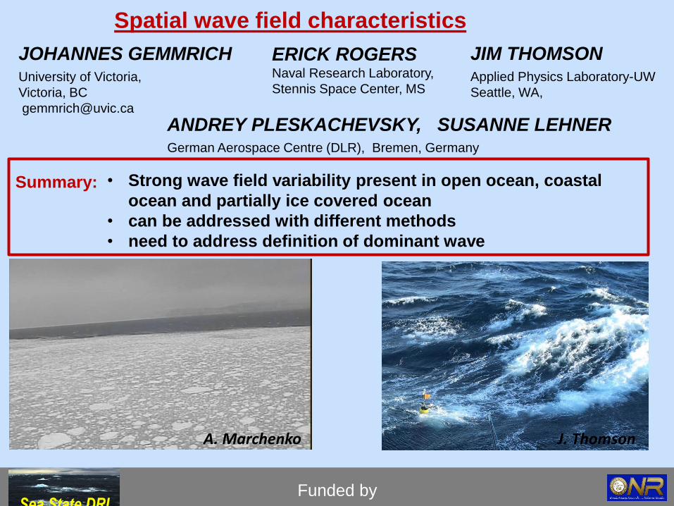
(Original) motivation:

Non-stationarity of wave field affects rogue wave statistics

Assume wave height time series

with significant wave height Hs but

2 stationary halves:

(Hs is always calculated from entire

record length)

Rogue wave occurrence in a non-

stationary record of two equal

length parts (coloured lines) is

much higher than if the record

were treated as 2 stationary parts

(black).

𝐻12 = 𝐻𝑠

2 1 + 𝜀𝐻22 = 𝐻𝑠

2 1 − 𝜀

𝑃𝜂

𝐻𝑠> 𝑧 =

1

2𝑒𝑥𝑝

−8𝑧2

1 + 𝜀+ 𝑒𝑥𝑝

−8𝑧2

1 − 𝜀

What about spatial inhomogeneity of wave field?

P

From Gemmrich & Garrett, NHESS 2011

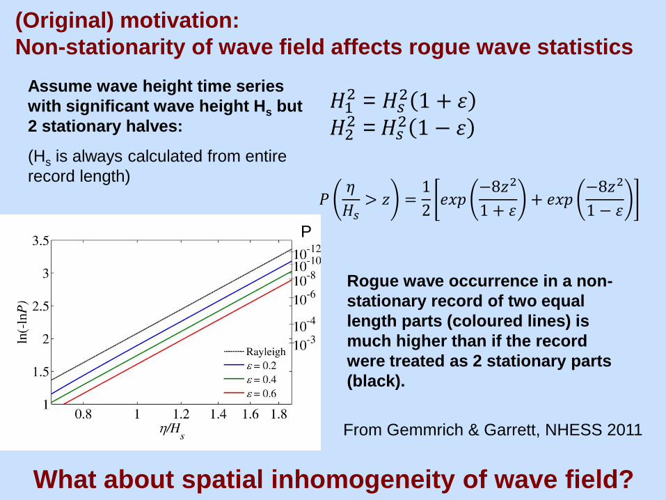
TerraSAR-X (DLR)

Wind Sea State Ice and Icebergs

• Sunlight independent (active sensor)

• Signal penetrates the clouds

• 1.25m resolution

• Swath width: 30 km

Methods (remote sensing):

Empirical algorithms for retrieval of

• significant wave height

• wind speed

(M. Bruck 2015; A. Pleskachevsky 2015)

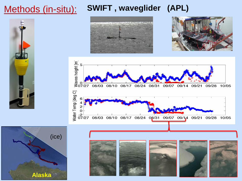
SWIFT , waveglider (APL)

(ice)

Alaska

Methods (in-situ):

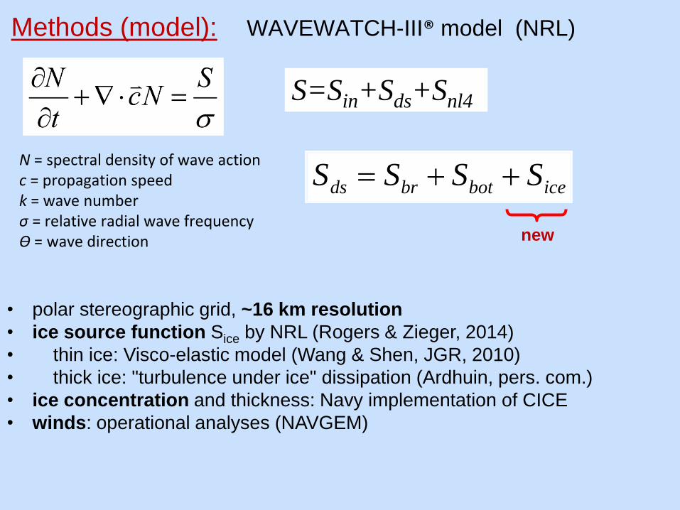
N = spectral density of wave actionc = propagation speed k = wave number σ = relative radial wave frequency ϴ = wave direction

• polar stereographic grid, ~16 km resolution

• ice source function Sice by NRL (Rogers & Zieger, 2014)

• thin ice: Visco-elastic model (Wang & Shen, JGR, 2010)

• thick ice: "turbulence under ice" dissipation (Ardhuin, pers. com.)

• ice concentration and thickness: Navy implementation of CICE

• winds: operational analyses (NAVGEM)

S=Sin+Sds+Snl4

new

icebotbrds SSSS

WAVEWATCH-III® model (NRL)Methods (model):

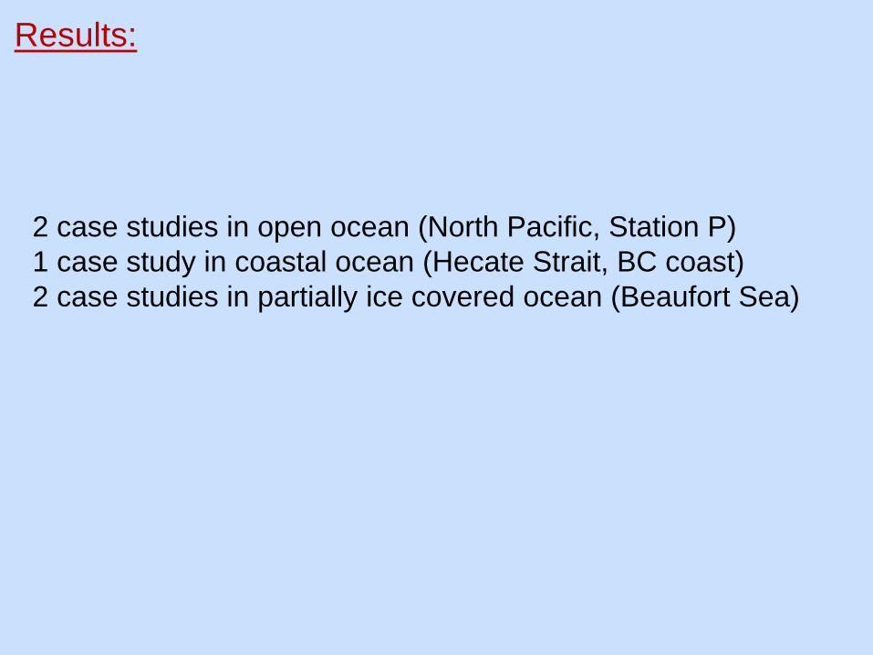
2 case studies in open ocean (North Pacific, Station P)

1 case study in coastal ocean (Hecate Strait, BC coast)

2 case studies in partially ice covered ocean (Beaufort Sea)

Results:

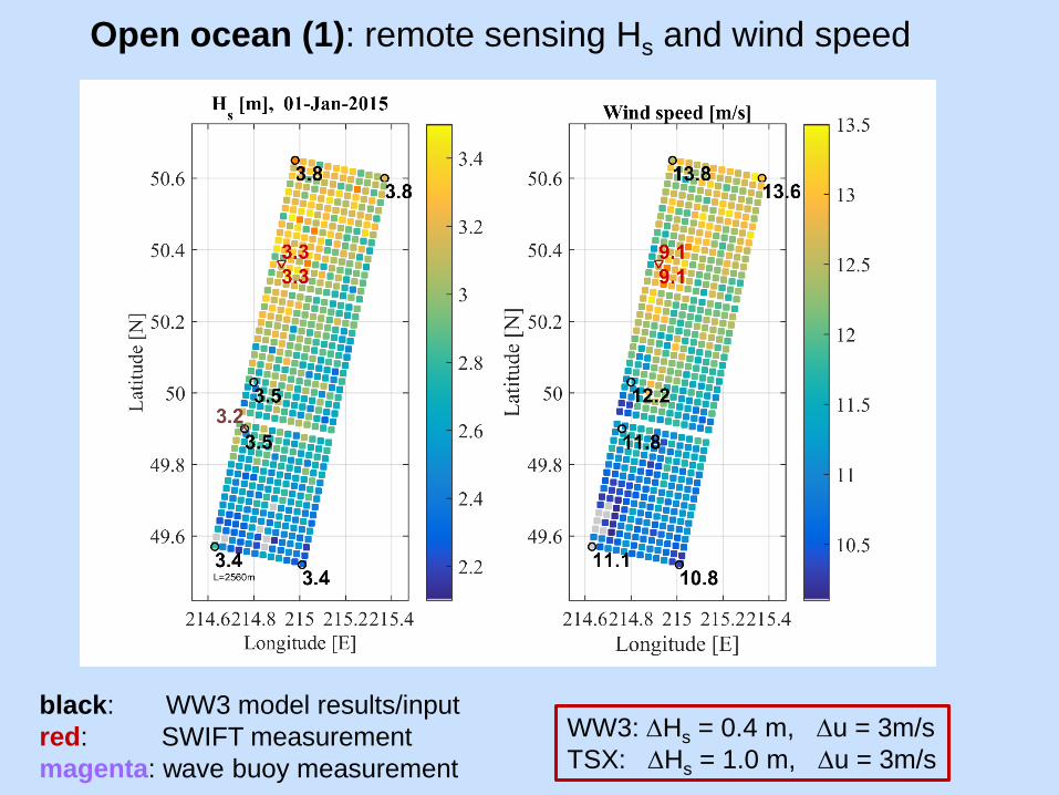
Open ocean (1): remote sensing Hs and wind speed

black: WW3 model results/input

red: SWIFT measurement

magenta: wave buoy measurement

WW3: DHs = 0.4 m, Du = 3m/s

TSX: DHs = 1.0 m, Du = 3m/s

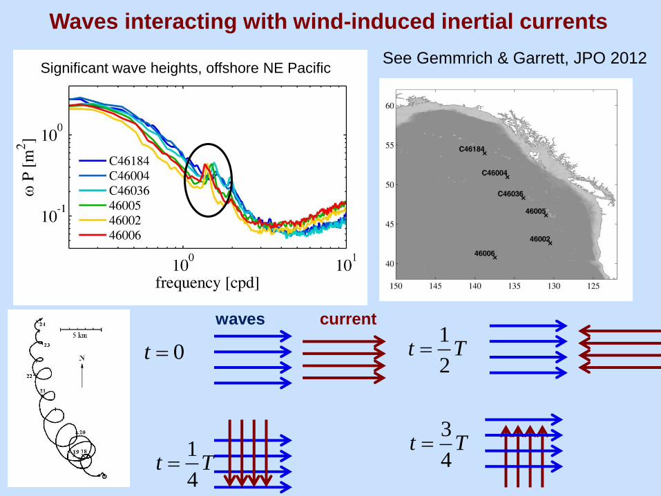
Significant wave heights, offshore NE Pacific

waves current

Waves interacting with wind-induced inertial currents

0t

1

4t T

1

2t T

3

4t T

See Gemmrich & Garrett, JPO 2012

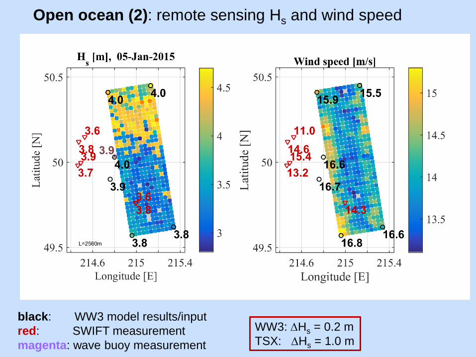
Open ocean (2): remote sensing Hs and wind speed

black: WW3 model results/input

red: SWIFT measurement

magenta: wave buoy measurement

WW3: DHs = 0.2 m

TSX: DHs = 1.0 m

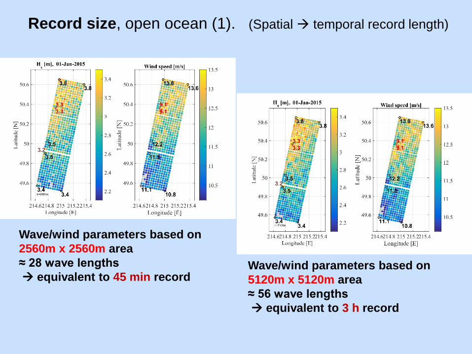
Record size, open ocean (1). (Spatial temporal record length)

Wave/wind parameters based on

2560m x 2560m area

≈ 28 wave lengths

equivalent to 45 min recordWave/wind parameters based on

5120m x 5120m area

≈ 56 wave lengths

equivalent to 3 h record

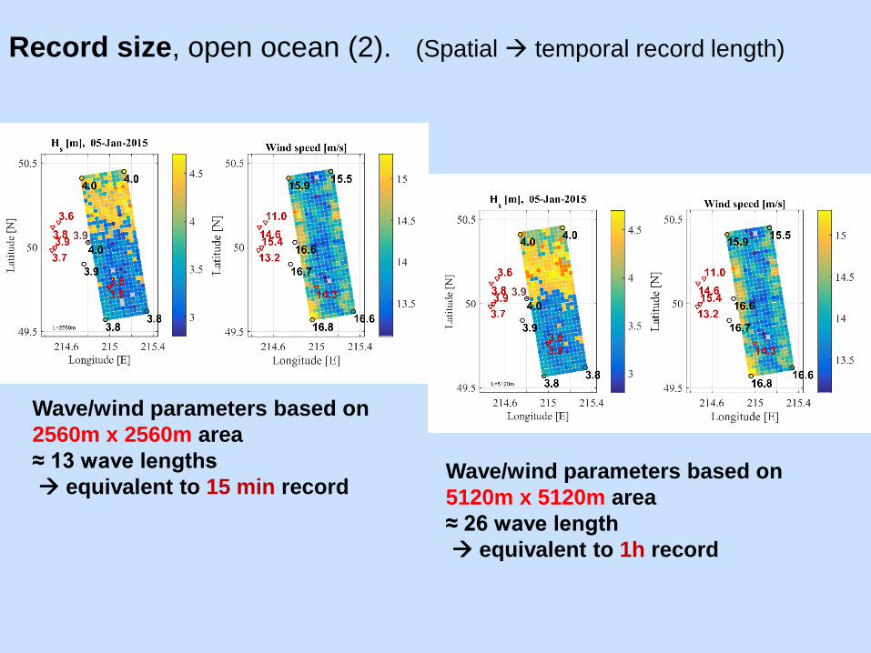
Record size, open ocean (2). (Spatial temporal record length)

Wave/wind parameters based on

2560m x 2560m area

≈ 13 wave lengths

equivalent to 15 min recordWave/wind parameters based on

5120m x 5120m area

≈ 26 wave length

equivalent to 1h record

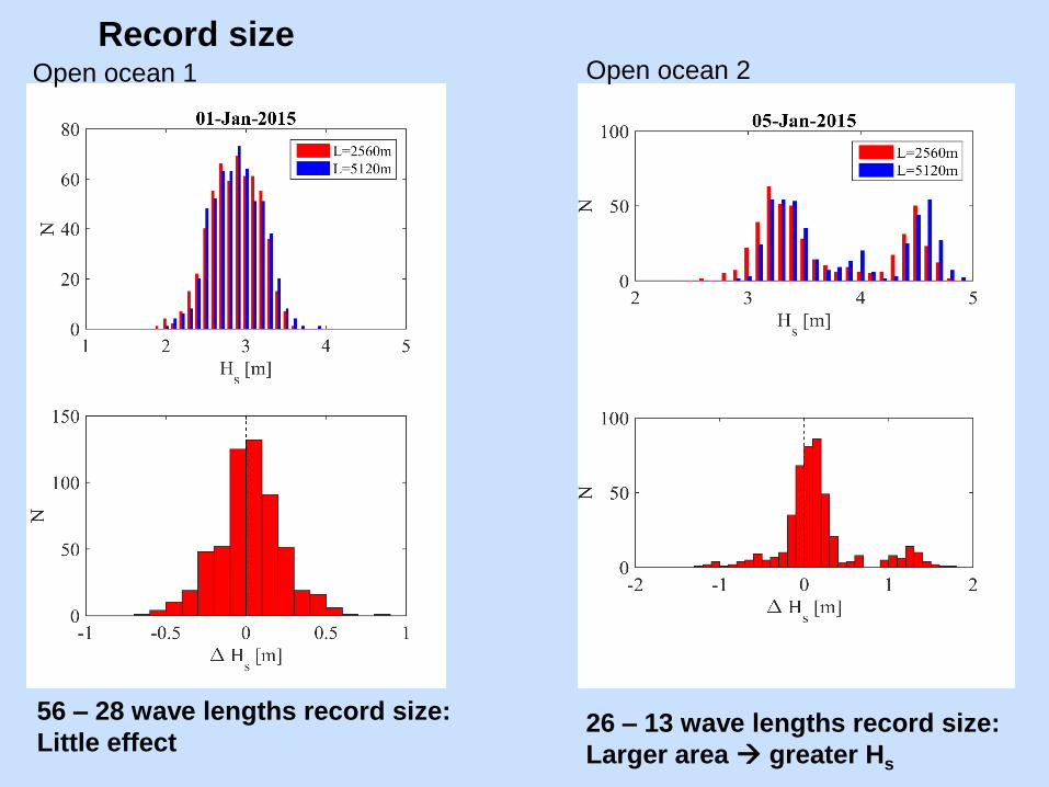
Record size

56 – 28 wave lengths record size:

Little effect26 – 13 wave lengths record size:

Larger area greater Hs

Open ocean 1 Open ocean 2

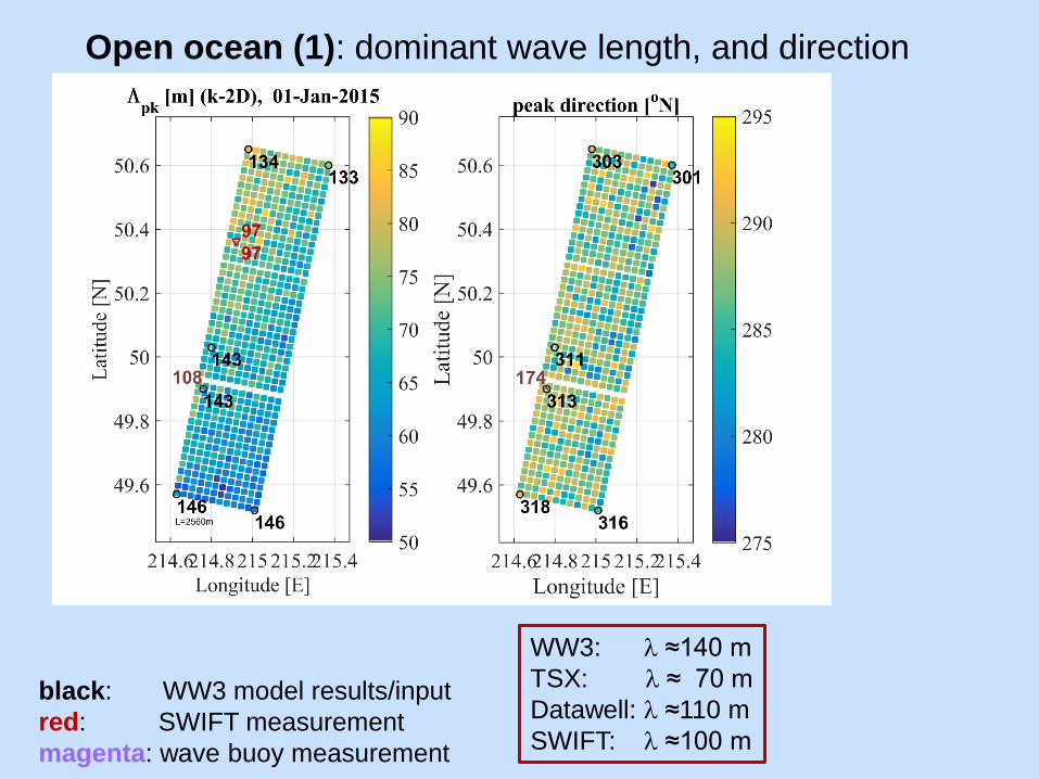
Open ocean (1): dominant wave length, and direction

black: WW3 model results/input

red: SWIFT measurement

magenta: wave buoy measurement

WW3: l ≈140 m

TSX: l ≈ 70 m

Datawell: l ≈110 m

SWIFT: l ≈100 m

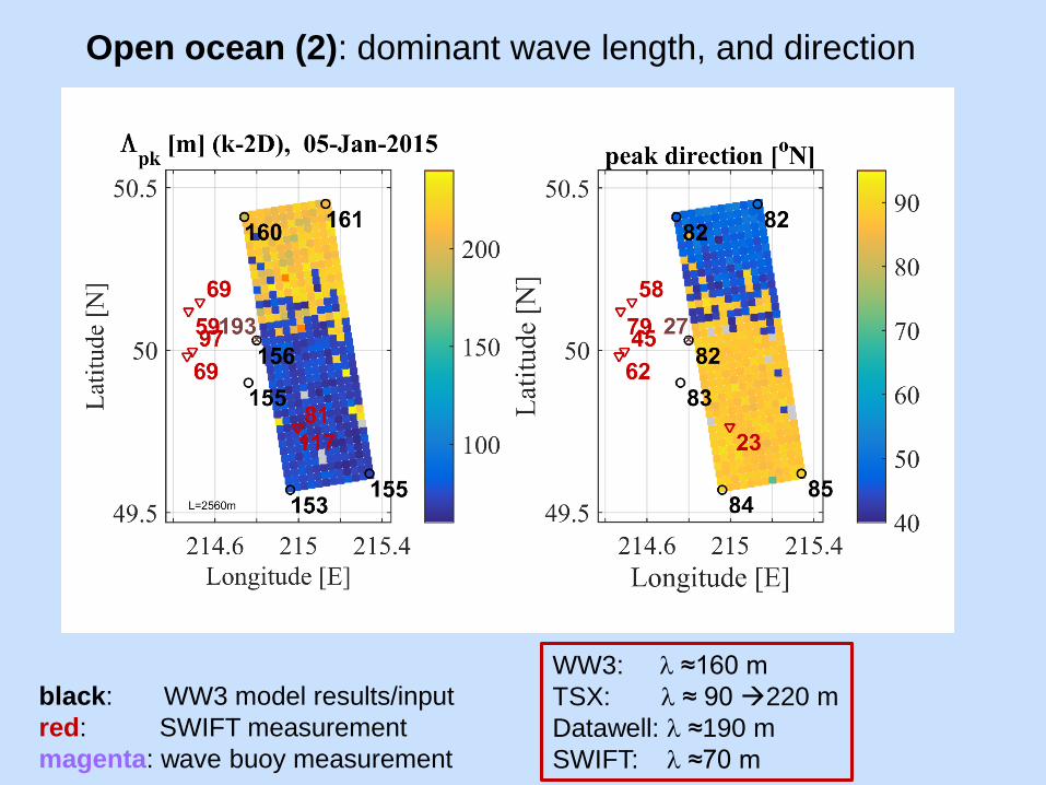
Open ocean (2): dominant wave length, and direction

black: WW3 model results/input

red: SWIFT measurement

magenta: wave buoy measurement

WW3: l ≈160 m

TSX: l ≈ 90 220 m

Datawell: l ≈190 m

SWIFT: l ≈70 m

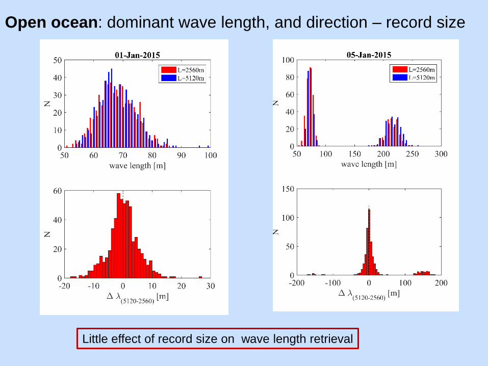
Open ocean: dominant wave length, and direction – record size

Little effect of record size on wave length retrieval

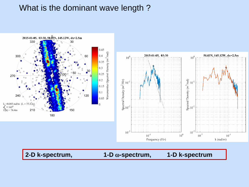
What is the dominant wave length ?

2-D k-spectrum, 1-D w-spectrum, 1-D k-spectrum

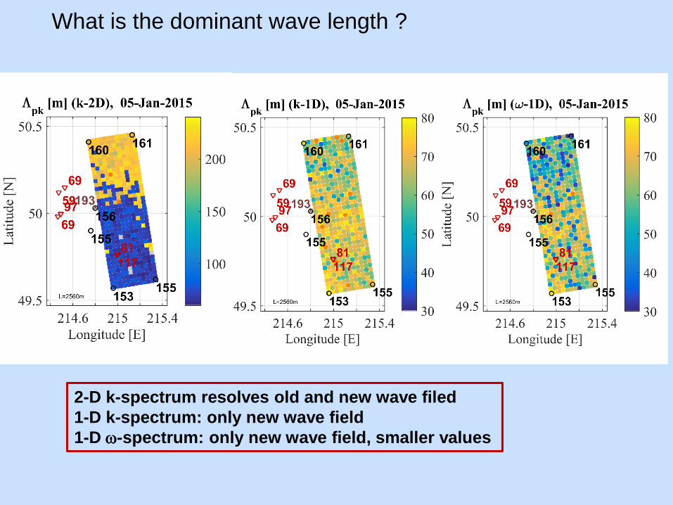
What is the dominant wave length ?

2-D k-spectrum resolves old and new wave filed

1-D k-spectrum: only new wave field

1-D w-spectrum: only new wave field, smaller values

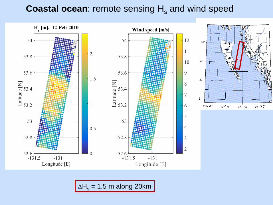
Coastal ocean: remote sensing Hs and wind speed

DHs = 1.5 m along 20km

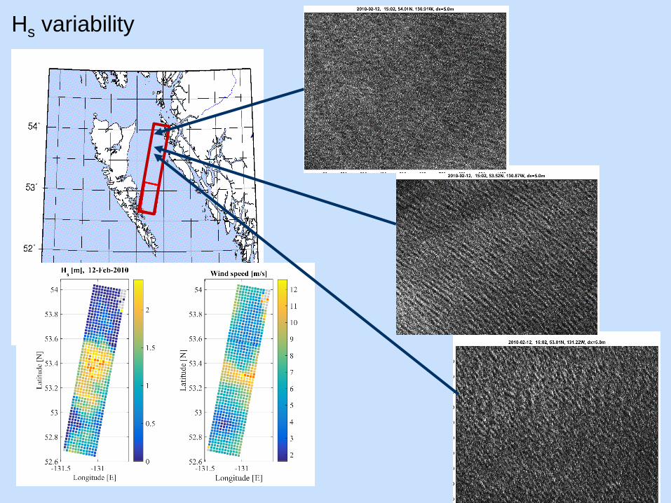
Hs variability

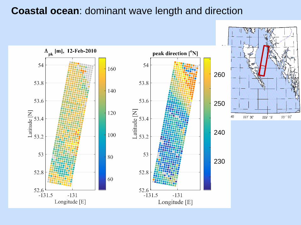
Coastal ocean: dominant wave length and direction

260

250

240

230

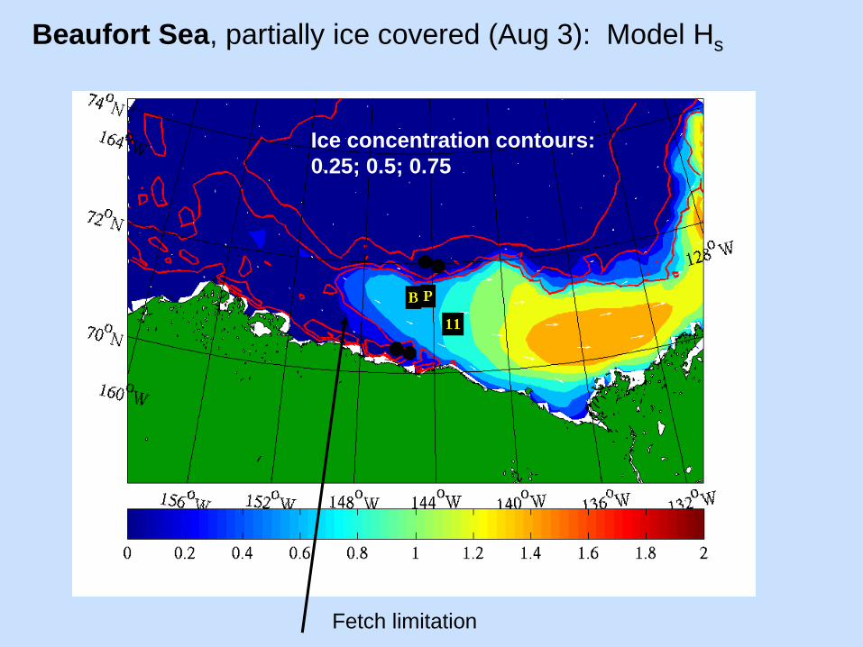
Beaufort Sea, partially ice covered (Aug 3): Model Hs

Ice concentration contours:

0.25; 0.5; 0.75

Fetch limitation

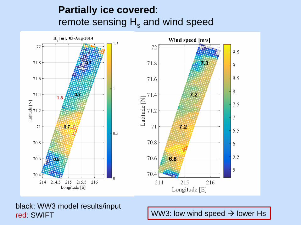
Partially ice covered:

remote sensing Hs and wind speed

black: WW3 model results/input

red: SWIFT WW3: low wind speed lower Hs

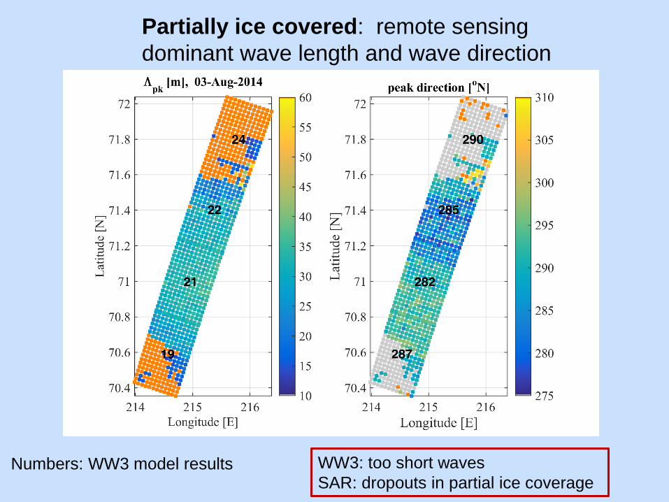
Partially ice covered: remote sensing

dominant wave length and wave direction

Numbers: WW3 model results WW3: too short waves

SAR: dropouts in partial ice coverage

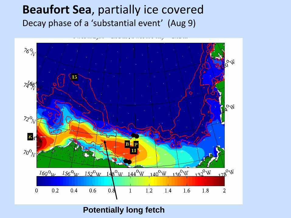
Beaufort Sea, partially ice covered Decay phase of a ‘substantial event’ (Aug 9)

Potentially long fetch

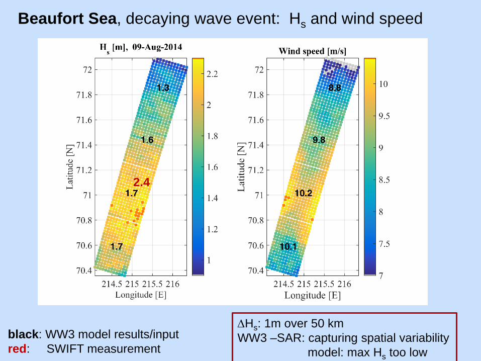
Beaufort Sea, decaying wave event: Hs and wind speed

black: WW3 model results/input

red: SWIFT measurement

DHs: 1m over 50 km

WW3 –SAR: capturing spatial variability

model: max Hs too low

2.4

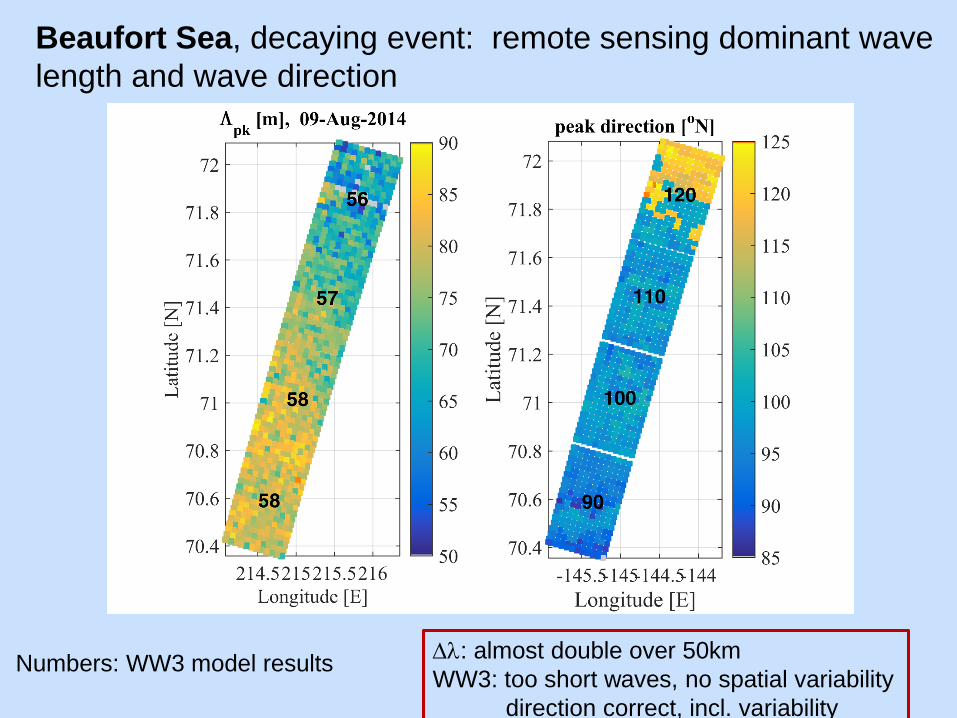
Beaufort Sea, decaying event: remote sensing dominant wave

length and wave direction

Numbers: WW3 model resultsDl: almost double over 50km

WW3: too short waves, no spatial variability

direction correct, incl. variability

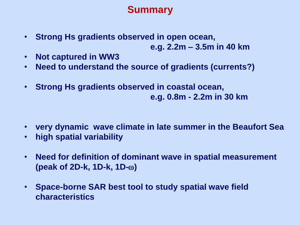
Summary

• Strong Hs gradients observed in open ocean,

e.g. 2.2m – 3.5m in 40 km

• Not captured in WW3

• Need to understand the source of gradients (currents?)

• Strong Hs gradients observed in coastal ocean,

e.g. 0.8m - 2.2m in 30 km

• very dynamic wave climate in late summer in the Beaufort Sea

• high spatial variability

• Need for definition of dominant wave in spatial measurement

(peak of 2D-k, 1D-k, 1D-w)

• Space-borne SAR best tool to study spatial wave field

characteristics