Embed Size (px)
Citation preview
8/3/2019 Andrew Rosenberg- Lecture 2.2: Linear Regression CSC 84020 - Machine Learning
http://slidepdf.com/reader/full/andrew-rosenberg-lecture-22-linear-regression-csc-84020-machine-learning 1/34
Lecture 2.2: Linear Regression
CSC 84020 - Machine Learning
Andrew Rosenberg
February 5, 2009

8/3/2019 Andrew Rosenberg- Lecture 2.2: Linear Regression CSC 84020 - Machine Learning
http://slidepdf.com/reader/full/andrew-rosenberg-lecture-22-linear-regression-csc-84020-machine-learning 2/34
Today
Linear Regression
8/3/2019 Andrew Rosenberg- Lecture 2.2: Linear Regression CSC 84020 - Machine Learning
http://slidepdf.com/reader/full/andrew-rosenberg-lecture-22-linear-regression-csc-84020-machine-learning 3/34
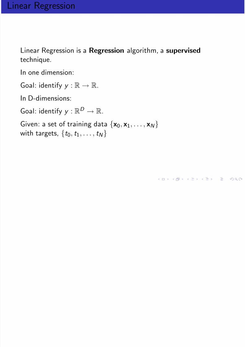
Linear Regression
Linear Regression is a Regression algorithm, a supervised
technique.
In one dimension:
Goal: identify y : R→ R.
In D-dimensions:
Goal: identify y : RD → R.
Given: a set of training data{
x0, x1, . . . , xN }with targets, {t 0, t 1, . . . , t N }
8/3/2019 Andrew Rosenberg- Lecture 2.2: Linear Regression CSC 84020 - Machine Learning
http://slidepdf.com/reader/full/andrew-rosenberg-lecture-22-linear-regression-csc-84020-machine-learning 4/34
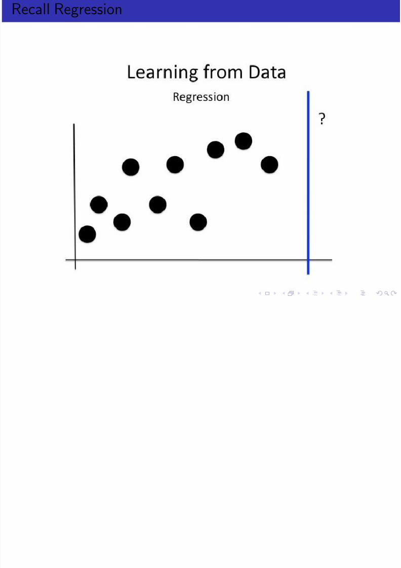
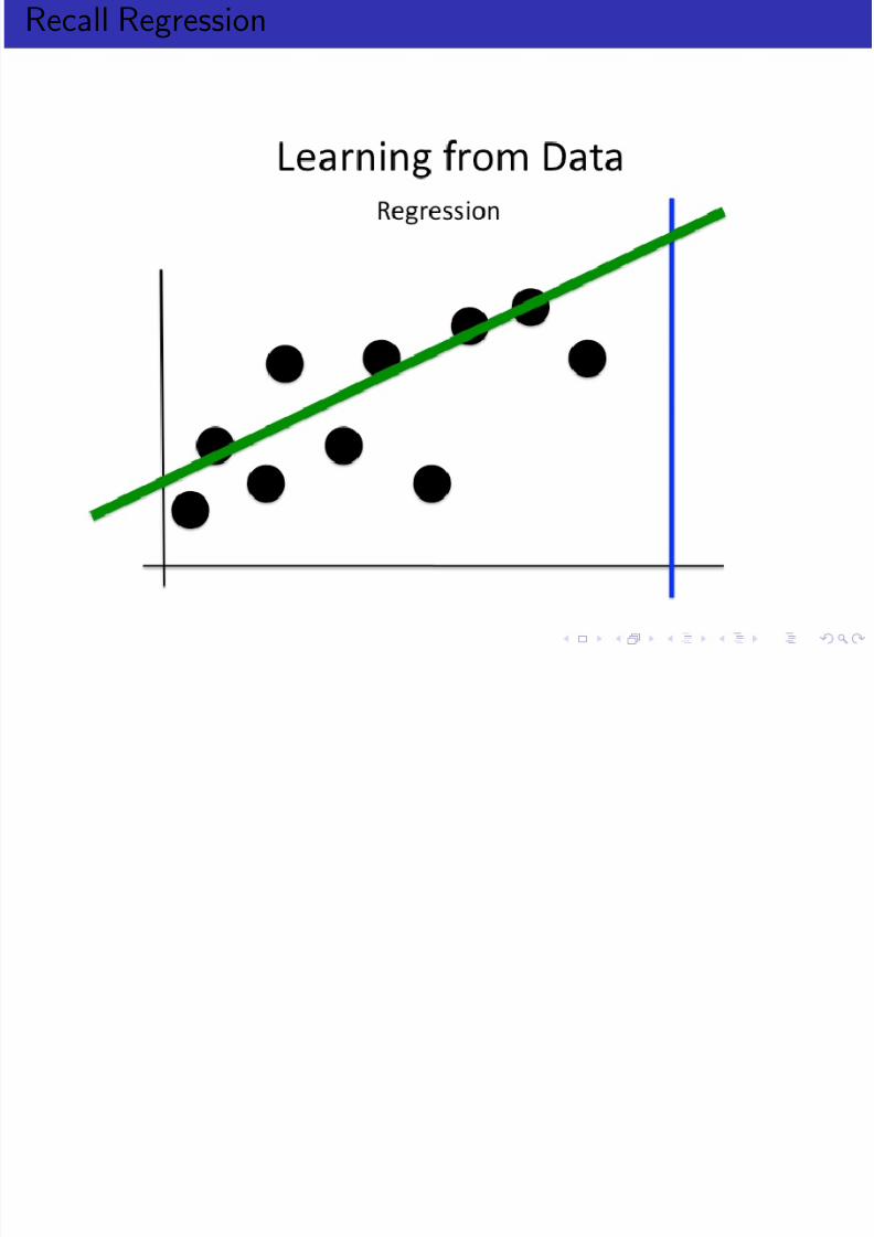
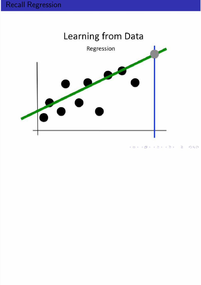
Recall Regression
8/3/2019 Andrew Rosenberg- Lecture 2.2: Linear Regression CSC 84020 - Machine Learning
http://slidepdf.com/reader/full/andrew-rosenberg-lecture-22-linear-regression-csc-84020-machine-learning 5/34
Recall Regression
8/3/2019 Andrew Rosenberg- Lecture 2.2: Linear Regression CSC 84020 - Machine Learning
http://slidepdf.com/reader/full/andrew-rosenberg-lecture-22-linear-regression-csc-84020-machine-learning 6/34
Recall Regression
D fi h bl
8/3/2019 Andrew Rosenberg- Lecture 2.2: Linear Regression CSC 84020 - Machine Learning
http://slidepdf.com/reader/full/andrew-rosenberg-lecture-22-linear-regression-csc-84020-machine-learning 7/34
Define the problem
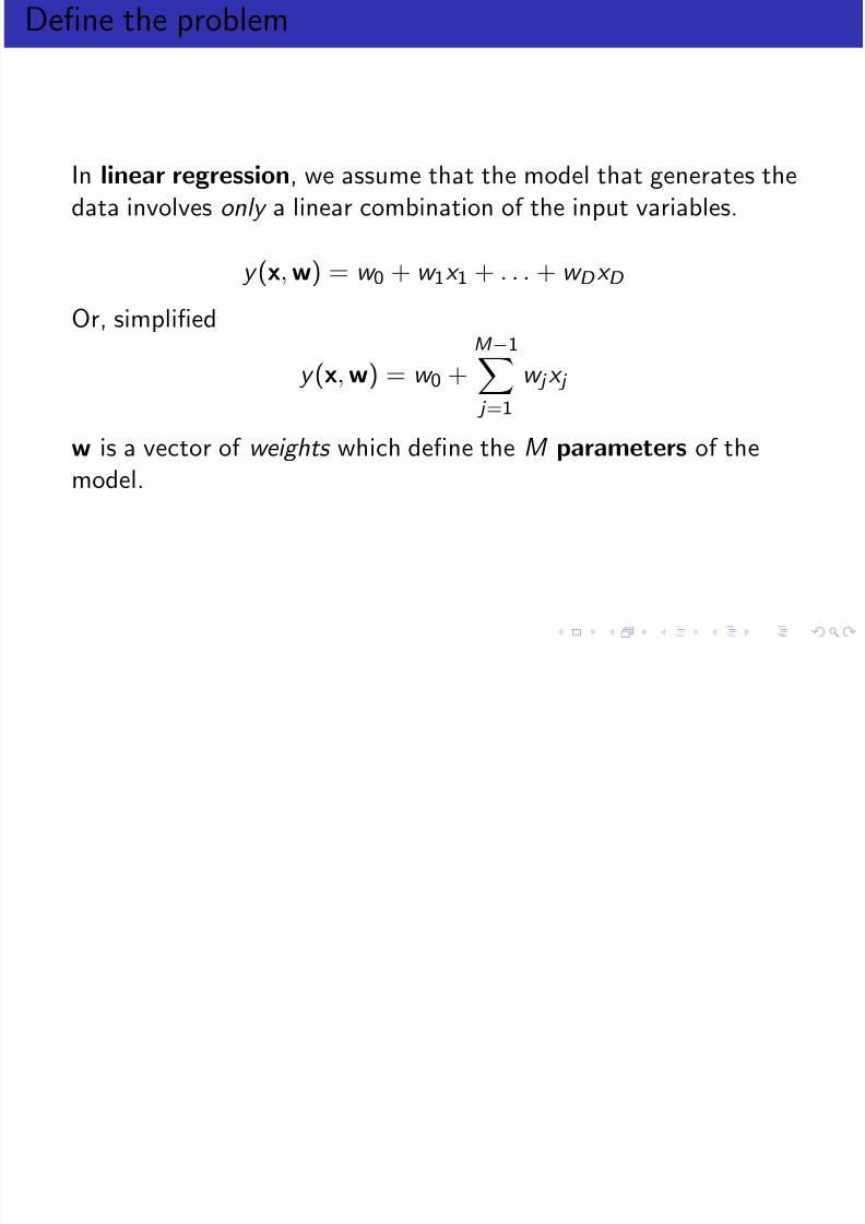
In linear regression, we assume that the model that generates thedata involves only a linear combination of the input variables.
y (x, w) = w 0 + w 1x 1 + . . . + w D x D
Or, simplified
y (x, w) = w 0 +M −1 j =1
w j x j
w is a vector of weights which define the M parameters of themodel.
O i i i
8/3/2019 Andrew Rosenberg- Lecture 2.2: Linear Regression CSC 84020 - Machine Learning
http://slidepdf.com/reader/full/andrew-rosenberg-lecture-22-linear-regression-csc-84020-machine-learning 8/34
Optimization
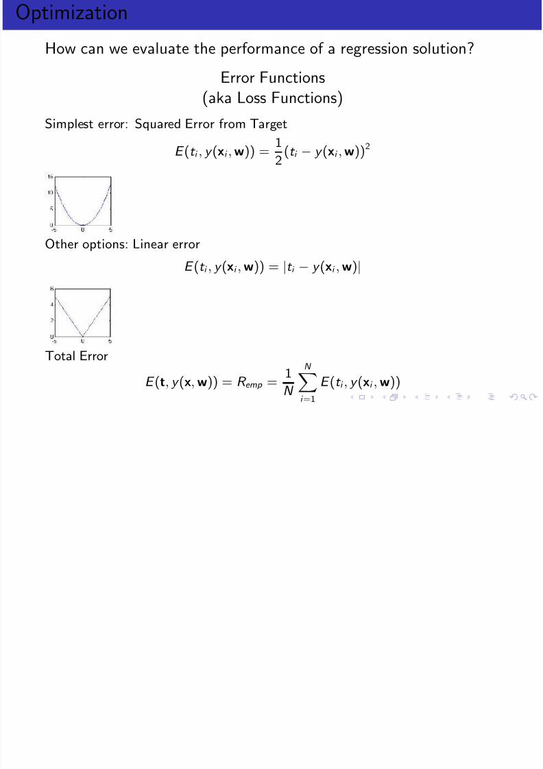
How can we evaluate the performance of a regression solution?
Error Functions
(aka Loss Functions)Simplest error: Squared Error from Target
E (t i , y (xi , w)) =1
2(t i − y (xi , w))2
Other options: Linear error
E (t i , y (xi , w)) = |t i − y (xi , w)|
Total Error
E (t, y (x, w)) = R emp = 1N
N
Xi =1
E (t i , y (xi , w))
8/3/2019 Andrew Rosenberg- Lecture 2.2: Linear Regression CSC 84020 - Machine Learning
http://slidepdf.com/reader/full/andrew-rosenberg-lecture-22-linear-regression-csc-84020-machine-learning 9/34
Lik lih d f t
8/3/2019 Andrew Rosenberg- Lecture 2.2: Linear Regression CSC 84020 - Machine Learning
http://slidepdf.com/reader/full/andrew-rosenberg-lecture-22-linear-regression-csc-84020-machine-learning 10/34
Likelihood of t
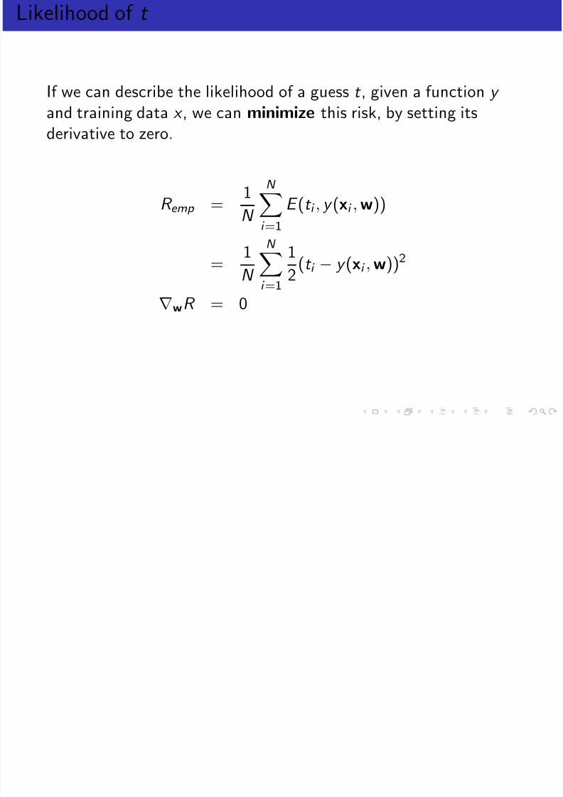
If we can describe the likelihood of a guess t , given a function y and training data x , we can minimize this risk, by setting itsderivative to zero.
R emp = 1N
N i =1
E (t i , y (xi , w))
=1
N
N
i =11
2(t i − y (xi , w))2
∇wR = 0
Lik lih d d Risk
8/3/2019 Andrew Rosenberg- Lecture 2.2: Linear Regression CSC 84020 - Machine Learning
http://slidepdf.com/reader/full/andrew-rosenberg-lecture-22-linear-regression-csc-84020-machine-learning 11/34
Likelihood and Risk
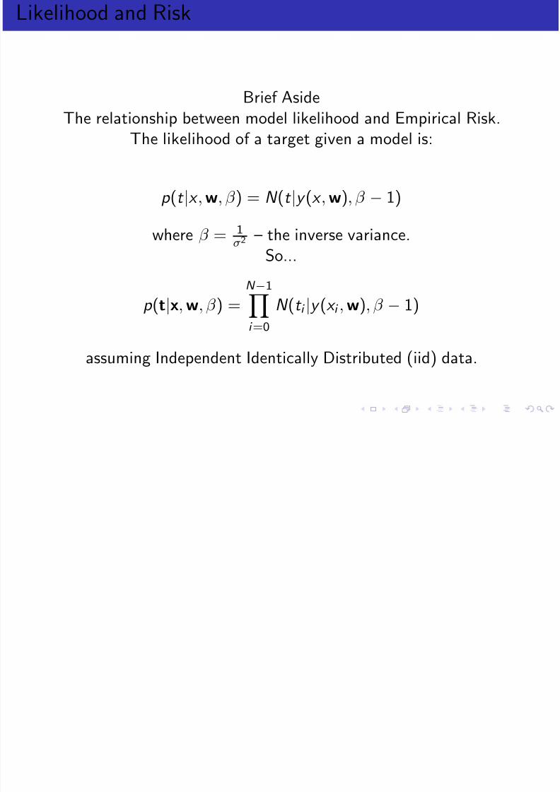
Brief AsideThe relationship between model likelihood and Empirical Risk.
The likelihood of a target given a model is:
p (t |x , w, β ) = N (t |y (x , w), β − 1)
where β = 1
σ2– the inverse variance.
So...
p (t|x, w, β ) =N −1i =0
N (t i |y (x i , w), β − 1)
assuming Independent Identically Distributed (iid) data.
Likelihood and Risk
8/3/2019 Andrew Rosenberg- Lecture 2.2: Linear Regression CSC 84020 - Machine Learning
http://slidepdf.com/reader/full/andrew-rosenberg-lecture-22-linear-regression-csc-84020-machine-learning 12/34
Likelihood and Risk
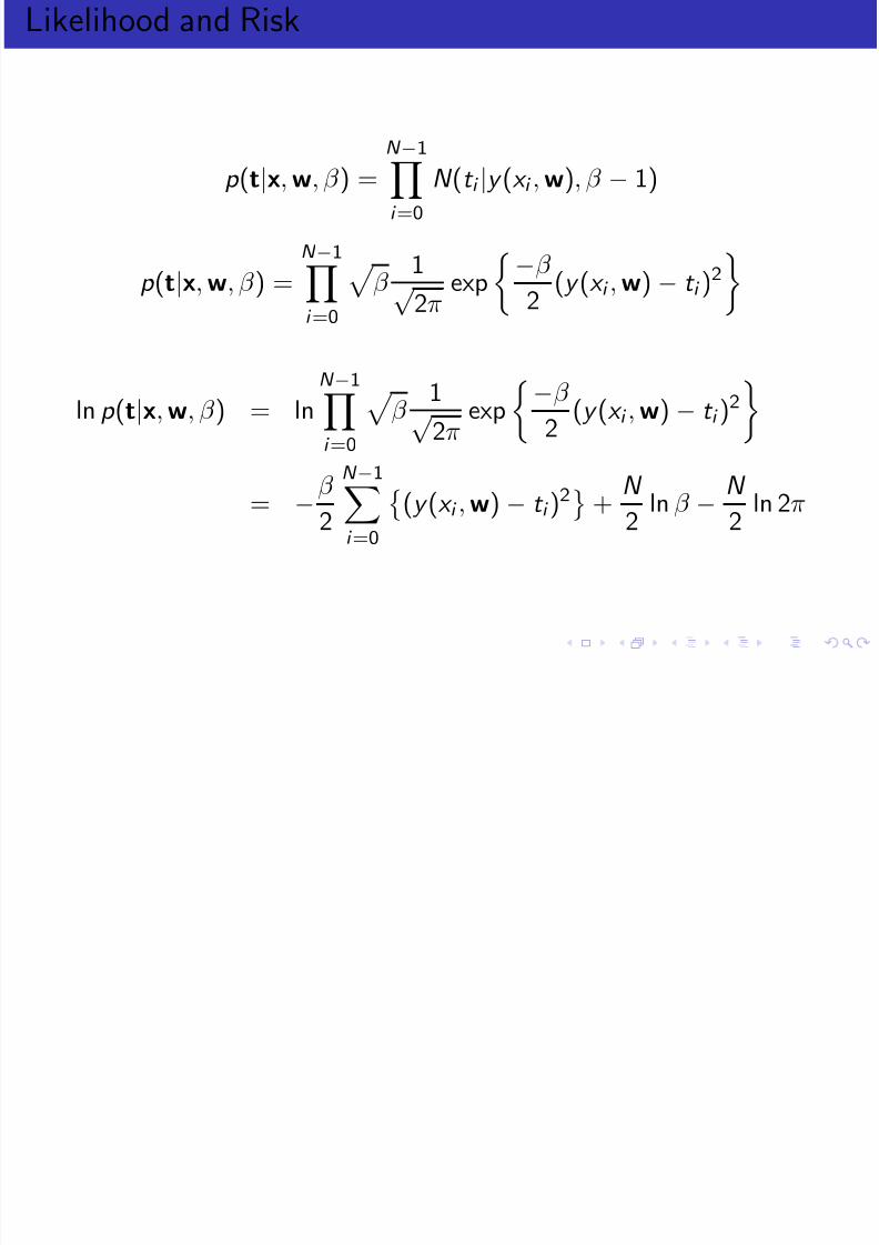
p (t|x, w, β ) =N −1
i =0
N (t i |y (x i , w), β − 1)
p (t
|x, w, β ) =
N −1
i =0
β 1
√2π
exp−β
2
(y (x i , w)
−t i )
2
ln p (t|x, w, β ) = lnN −1
i =0 β
1√2π
exp
−β
2(y (x i , w) − t i )
2
= −β
2
N −1i =0
(y (x i , w) − t i )
2
+N
2ln β − N
2ln 2π
8/3/2019 Andrew Rosenberg- Lecture 2.2: Linear Regression CSC 84020 - Machine Learning
http://slidepdf.com/reader/full/andrew-rosenberg-lecture-22-linear-regression-csc-84020-machine-learning 13/34
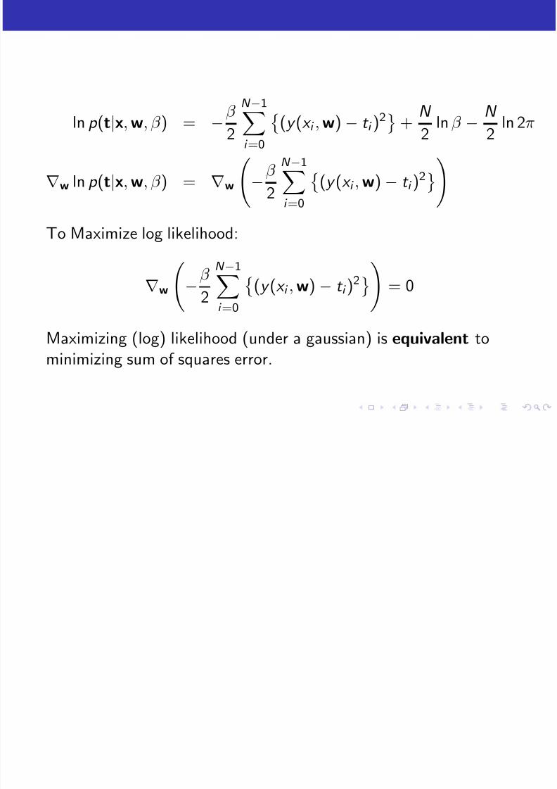
ln p (t|x, w, β ) = −β
2
N −1i =0
(y (x i , w) − t i )
2
+N
2ln β − N
2ln 2π
∇w ln p (t
|x, w, β ) =
∇w −
β
2
N −1
i =0
(y (x i , w)
−t i )
2To Maximize log likelihood:
∇w−
β
2
N −1i =0
(y (x i
,w) − t i )
2= 0
Maximizing (log) likelihood (under a gaussian) is equivalent tominimizing sum of squares error.
8/3/2019 Andrew Rosenberg- Lecture 2.2: Linear Regression CSC 84020 - Machine Learning
http://slidepdf.com/reader/full/andrew-rosenberg-lecture-22-linear-regression-csc-84020-machine-learning 14/34
Maximize the log likelihood
8/3/2019 Andrew Rosenberg- Lecture 2.2: Linear Regression CSC 84020 - Machine Learning
http://slidepdf.com/reader/full/andrew-rosenberg-lecture-22-linear-regression-csc-84020-machine-learning 15/34
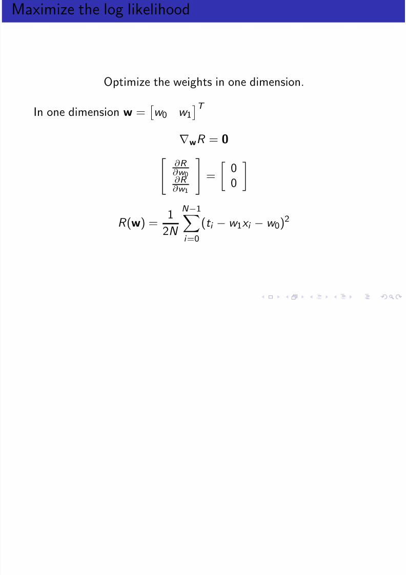
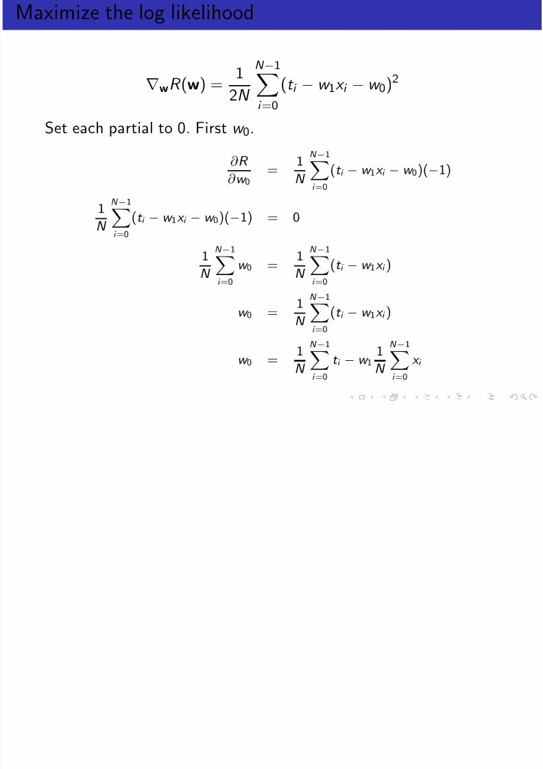
Maximize the log likelihood
∇wR (w) =
1
2N
N −1
i =0
(t i −w 1x i
−w 0)2
Set each partial to 0. First w 0.
∂ R
∂ w 0=
1
N
N −1X
i =0
(t i − w 1x i − w 0)(−1)
1
N
N −1X
i =0
(t i − w 1x i − w 0)(−1) = 0
1
N
N −1X
i =0
w 0 =1
N
N −1X
i =0
(t i − w 1x i )
w 0 =1
N
N −1X
i =0
(t i − w 1x i )
w 0 =1
N
N −1X
i =0
t i − w 11
N
N −1X
i =0
x i
Maximize the log likelihood
8/3/2019 Andrew Rosenberg- Lecture 2.2: Linear Regression CSC 84020 - Machine Learning
http://slidepdf.com/reader/full/andrew-rosenberg-lecture-22-linear-regression-csc-84020-machine-learning 16/34
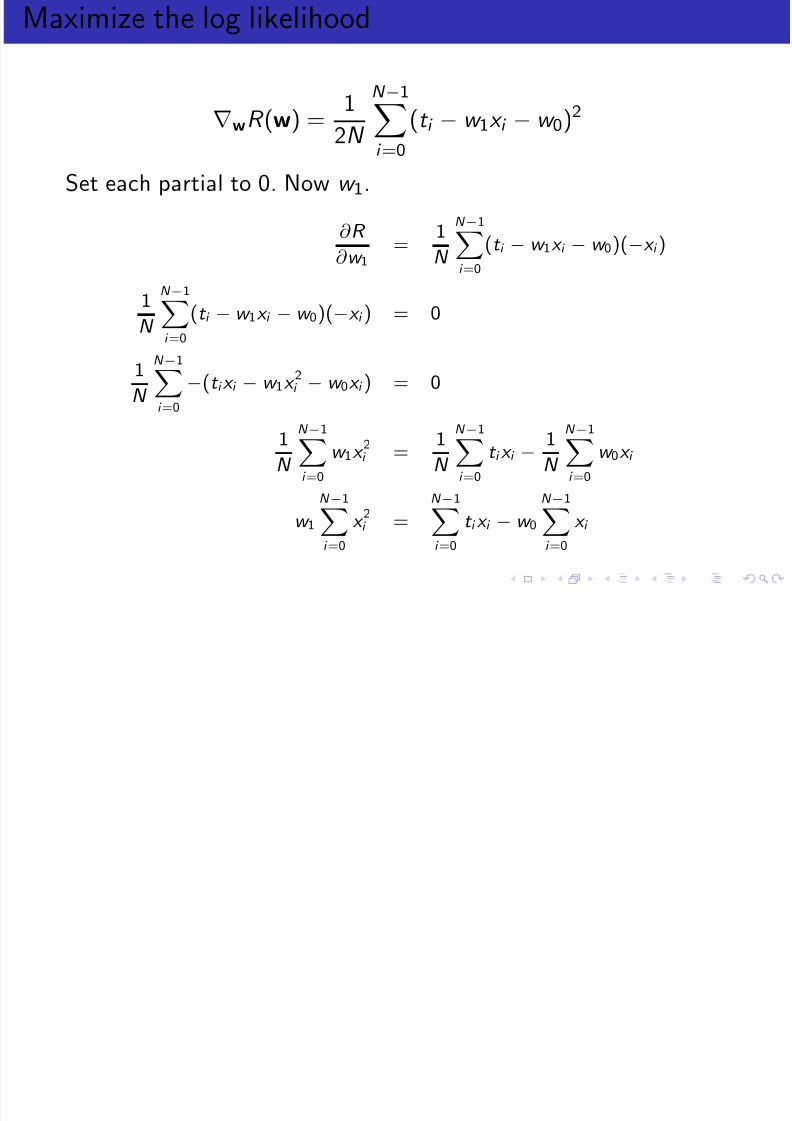
Maximize the log likelihood
∇wR (w) =
1
2N
N −1
i =0
(t i
−w 1x i
−w 0)2
Set each partial to 0. Now w 1.
∂ R
∂ w 1=
1
N
N −1X
i =0
(t i − w 1x i − w 0)(−x i )
1
N
N −1X
i =0
(t i −w 1x i −w 0)(−x i ) = 0
1
N
N −1X
i =0
−(t i x i − w 1x 2
i − w 0x i ) = 0
1
N
N −1X
i =0
w 1x 2
i =1
N
N −1X
i =0
t i x i −1
N
N −1X
i =0
w 0x i
w 1
N −1X
i =0
x 2
i =
N −1X
i =0
t i x i − w 0
N −1X
i =0
x i
Maximize the log likelihood
8/3/2019 Andrew Rosenberg- Lecture 2.2: Linear Regression CSC 84020 - Machine Learning
http://slidepdf.com/reader/full/andrew-rosenberg-lecture-22-linear-regression-csc-84020-machine-learning 17/34
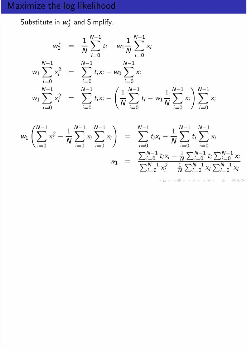
Maximize the log likelihood
Substitute in w ∗0
and Simplify.
w ∗
0 =1
N
N −1i =0
t i − w 11
N
N −1i =0
x i
w 1
N −1
i =0x 2i =
N −1
i =0t i x i − w 0
N −1
i =0x i
w 1
N −1i =0
x 2i =N −1i =0
t i x i −
1
N
N −1i =0
t i − w 11
N
N −1i =0
x i
N −1i =0
x i
w 1N −1
i =0
x 2i − 1N
N −1i =0
x i
N −1i =0
x i
=
N −1i =0
t i x i − 1N
N −1i =0
t i
N −1i =0
x i
w 1 =
N −1i =0 t i x i − 1
N
N −1i =0 t i
N −1i =0 x i
N −1i =0 x 2i
−1
N N −1i =0 x i N −1
i =0 x i
Maximized Log likelihood
8/3/2019 Andrew Rosenberg- Lecture 2.2: Linear Regression CSC 84020 - Machine Learning
http://slidepdf.com/reader/full/andrew-rosenberg-lecture-22-linear-regression-csc-84020-machine-learning 18/34
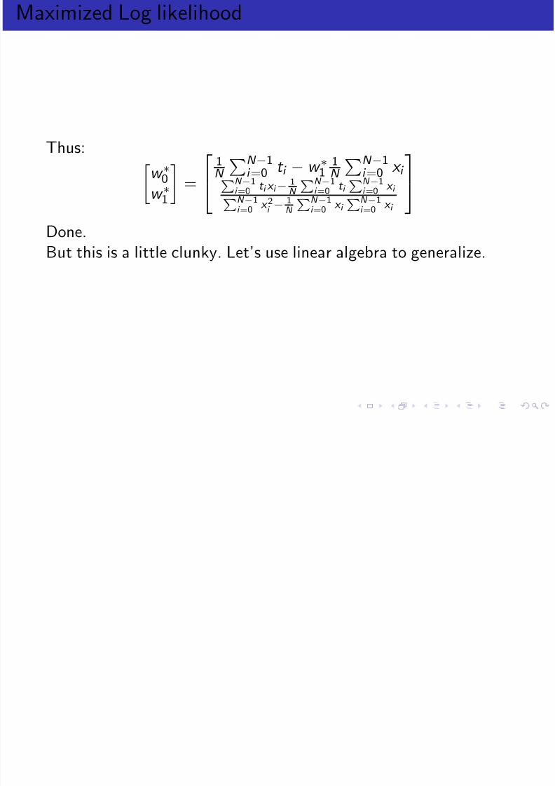
Maximized Log likelihood
Thus:
w ∗
0
w ∗
1 =
1
N N −1i =0 t i − w ∗
1
1
N N −1i =0 x i
PN −1i =0
t i x i −1
N
PN −1i =0
t i PN −1
i =0x i
PN −1
i =0x 2i −
1
N
PN −1
i =0x i P
N −1
i =0x i
Done.But this is a little clunky. Let’s use linear algebra to generalize.
8/3/2019 Andrew Rosenberg- Lecture 2.2: Linear Regression CSC 84020 - Machine Learning
http://slidepdf.com/reader/full/andrew-rosenberg-lecture-22-linear-regression-csc-84020-machine-learning 19/34
Extend to multiple dimensions
8/3/2019 Andrew Rosenberg- Lecture 2.2: Linear Regression CSC 84020 - Machine Learning
http://slidepdf.com/reader/full/andrew-rosenberg-lecture-22-linear-regression-csc-84020-machine-learning 20/34
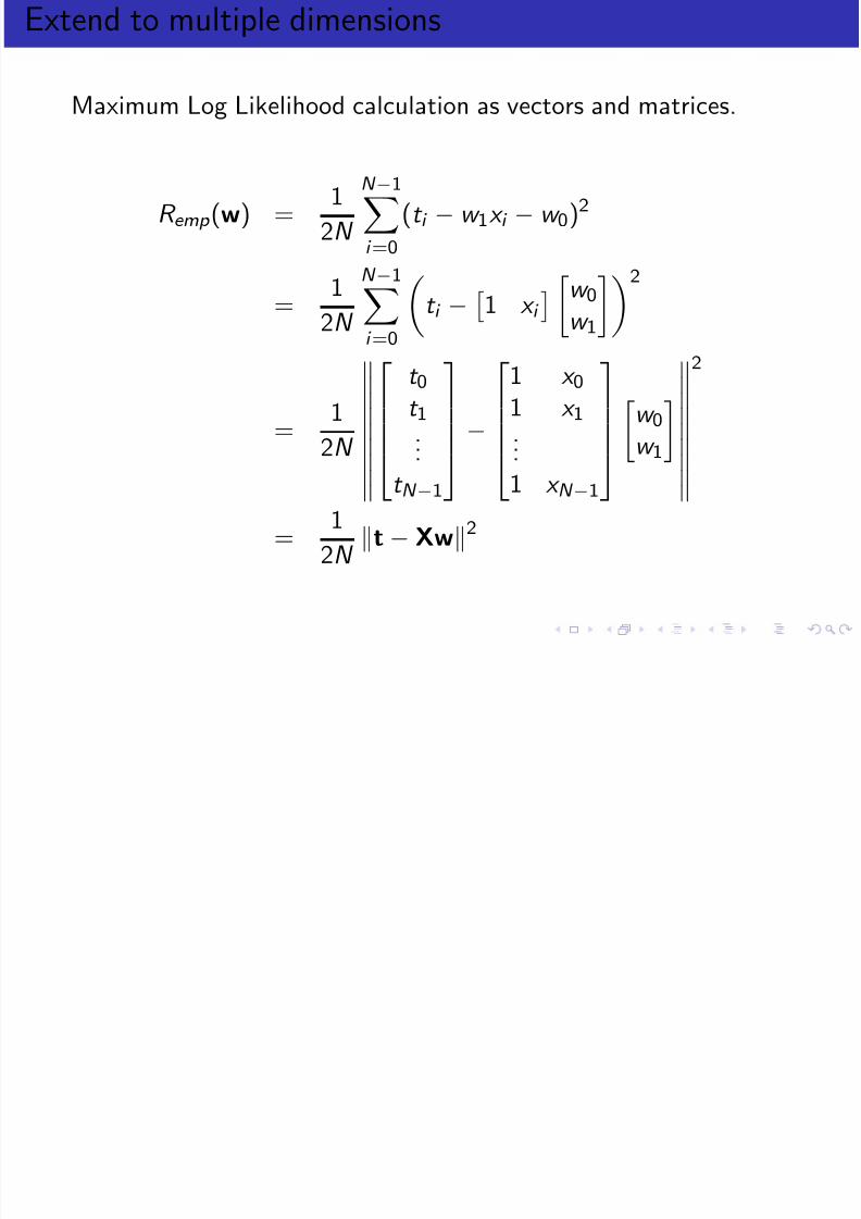
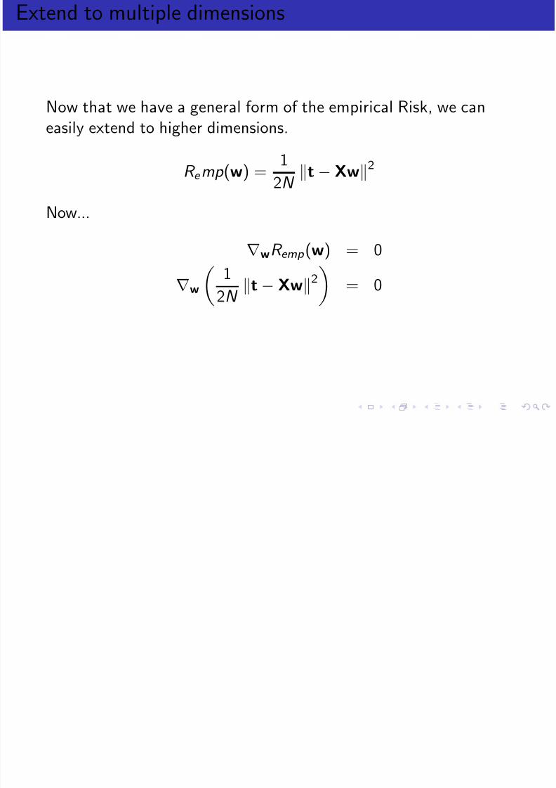
Extend to multiple dimensions
Now that we have a general form of the empirical Risk, we caneasily extend to higher dimensions.
R e mp (w) =1
2N t − Xw2
Now...
∇wR emp (w) = 0
∇w 1
2N t−
Xw2 = 0
General form of Risk minimization
8/3/2019 Andrew Rosenberg- Lecture 2.2: Linear Regression CSC 84020 - Machine Learning
http://slidepdf.com/reader/full/andrew-rosenberg-lecture-22-linear-regression-csc-84020-machine-learning 21/34
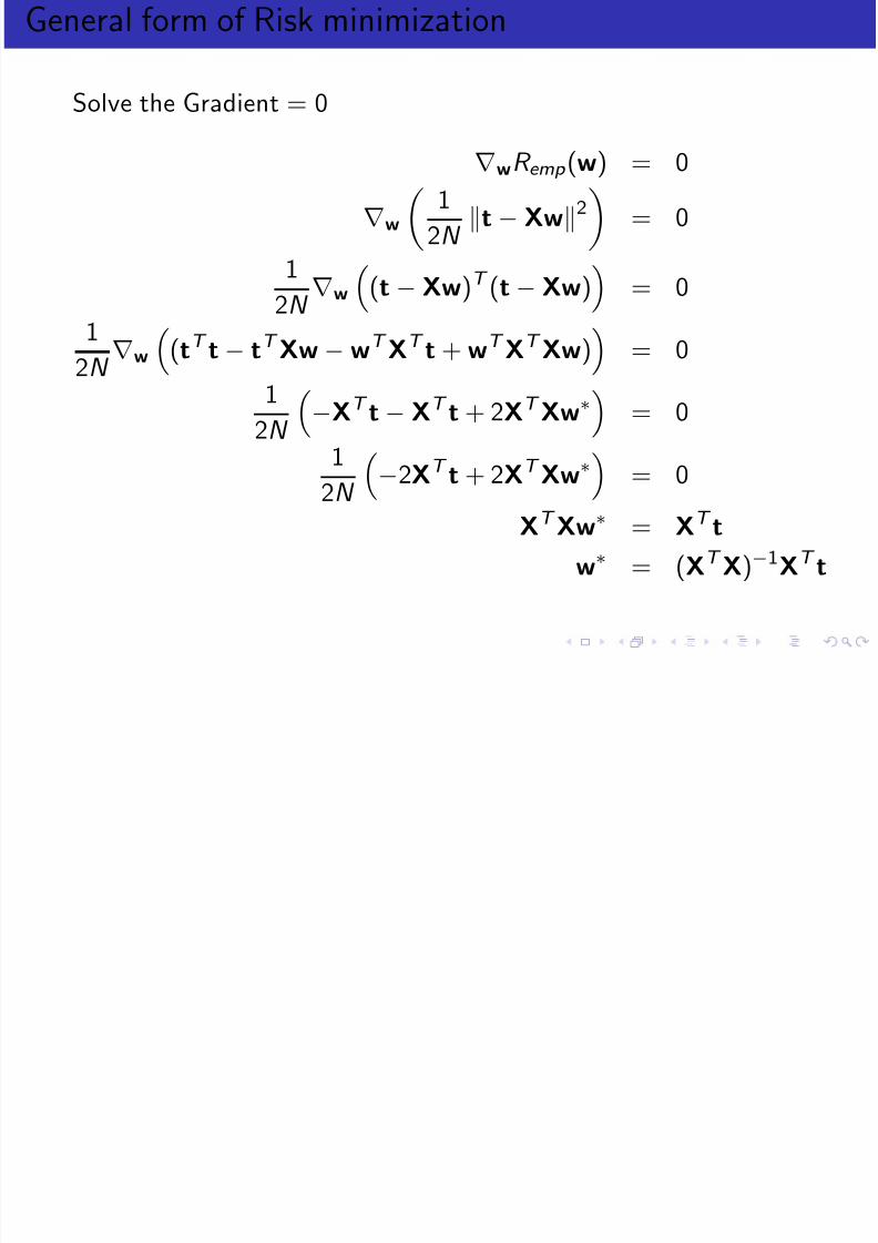
General form of Risk minimization
Solve the Gradient = 0
∇wR emp (w) = 0
∇w
1
2N t − Xw2
= 0
1
2N ∇w (t
−Xw)T (t
−Xw) = 0
1
2N ∇w
(tT t − tT Xw − wT XT t + wT XT Xw)
= 0
1
2N −XT t − XT t + 2XT Xw∗
= 0
12N
−2XT t + 2XT Xw∗
= 0
XT Xw∗ = XT t
w∗ = (XT X)−1XT t
Extension to fitting a line to a curve
8/3/2019 Andrew Rosenberg- Lecture 2.2: Linear Regression CSC 84020 - Machine Learning
http://slidepdf.com/reader/full/andrew-rosenberg-lecture-22-linear-regression-csc-84020-machine-learning 22/34
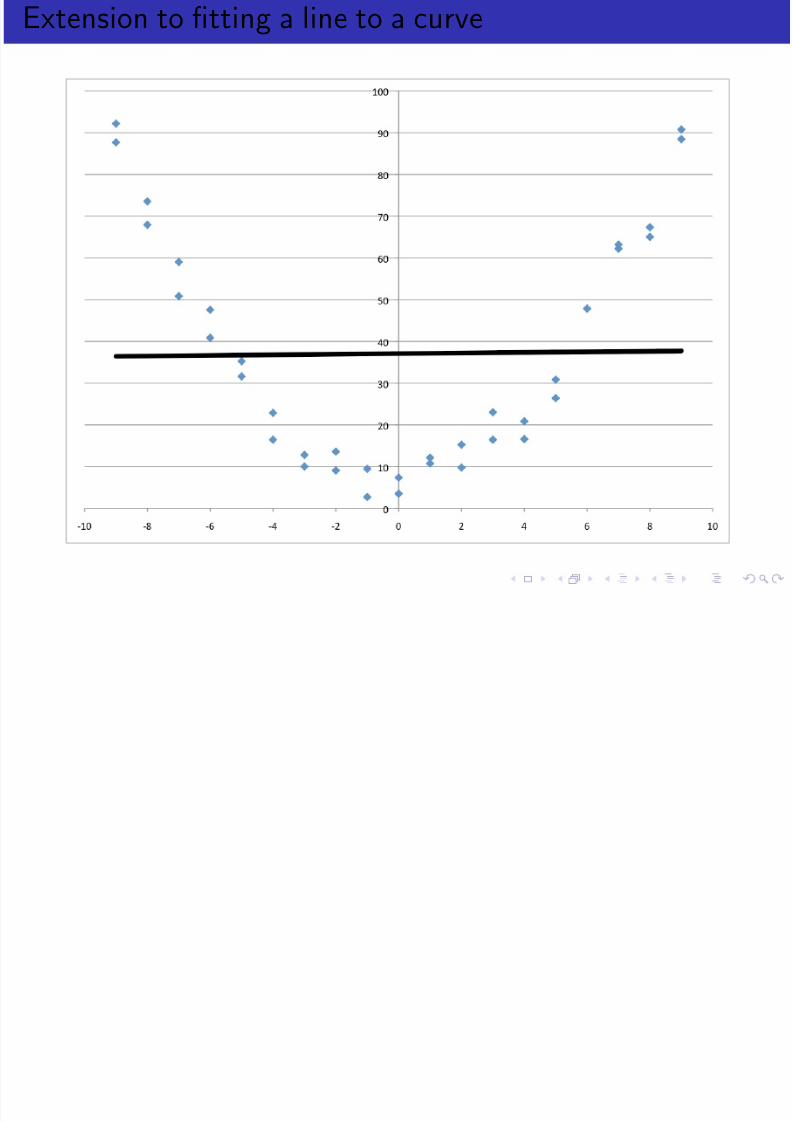
Extension to fitting a line to a curve
Polynomial Regression
8/3/2019 Andrew Rosenberg- Lecture 2.2: Linear Regression CSC 84020 - Machine Learning
http://slidepdf.com/reader/full/andrew-rosenberg-lecture-22-linear-regression-csc-84020-machine-learning 23/34
y g
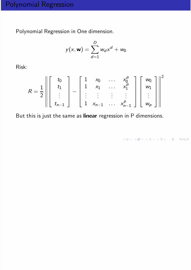
Polynomial Regression in One dimension.
y (x , w) =D
d =1
w d x d + w 0
Risk:
R =1
2
t 0t 1...
t n−1
−
1 x 0 . . . x
p 0
1 x 1 . . . x p 1
......
......
1 x n−1 . . . x p n−1
w 0w 1
...
w p
2
But this is just the same as linear regression in P dimensions.
Polynomial Regression as Linear Regression
8/3/2019 Andrew Rosenberg- Lecture 2.2: Linear Regression CSC 84020 - Machine Learning
http://slidepdf.com/reader/full/andrew-rosenberg-lecture-22-linear-regression-csc-84020-machine-learning 24/34
y g g
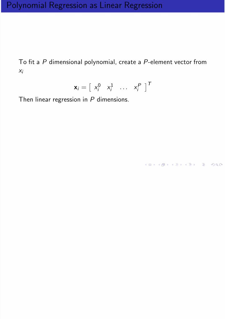
To fit a P dimensional polynomial, create a P -element vector from
x i
xi =x 0i x 1i . . . x P i
T Then linear regression in P dimensions.
How is this Linear regression?
8/3/2019 Andrew Rosenberg- Lecture 2.2: Linear Regression CSC 84020 - Machine Learning
http://slidepdf.com/reader/full/andrew-rosenberg-lecture-22-linear-regression-csc-84020-machine-learning 25/34
g
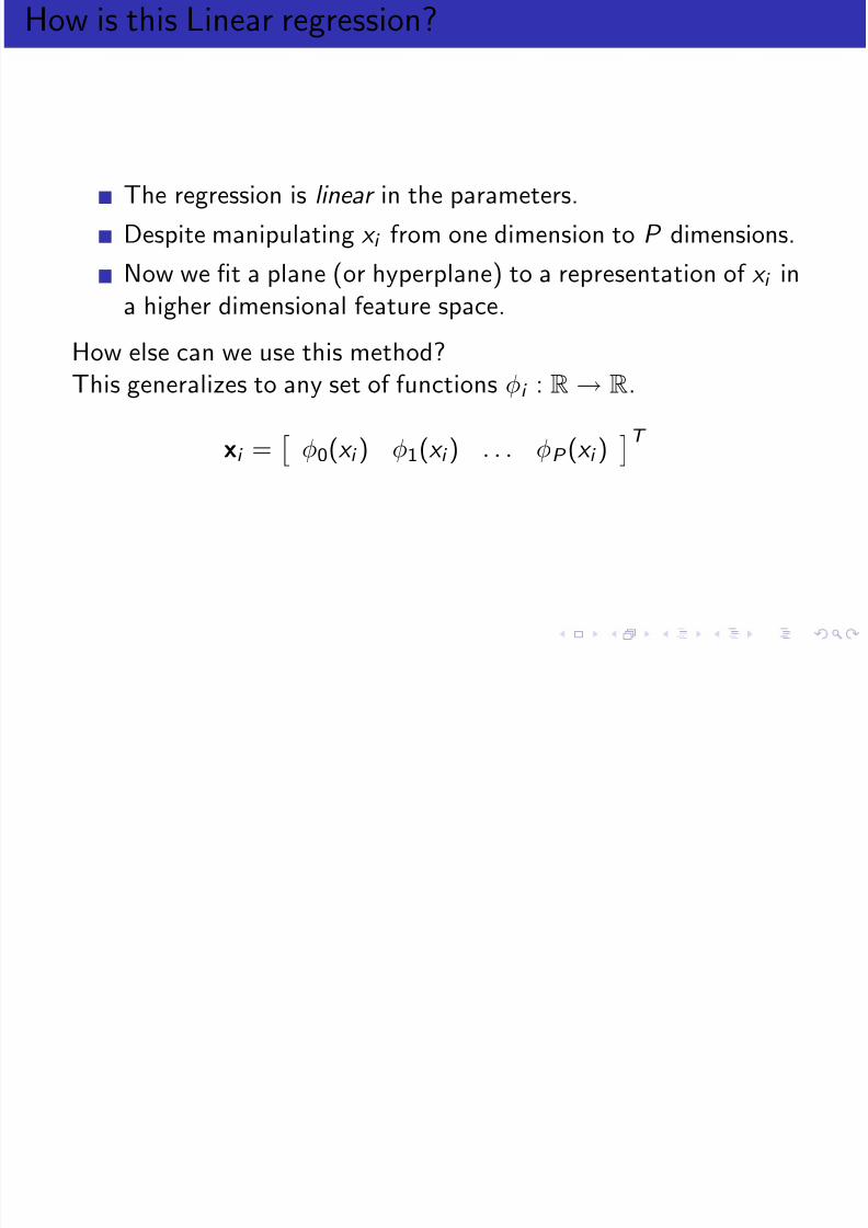
The regression is linear in the parameters.
Despite manipulating x i from one dimension to P dimensions.
Now we fit a plane (or hyperplane) to a representation of x i in
a higher dimensional feature space.How else can we use this method?This generalizes to any set of functions φi : R→ R.
xi =
φ0(x i )
φ1(x i )
. . . φP (x i )T
Basis functions as Feature Extraction
8/3/2019 Andrew Rosenberg- Lecture 2.2: Linear Regression CSC 84020 - Machine Learning
http://slidepdf.com/reader/full/andrew-rosenberg-lecture-22-linear-regression-csc-84020-machine-learning 26/34
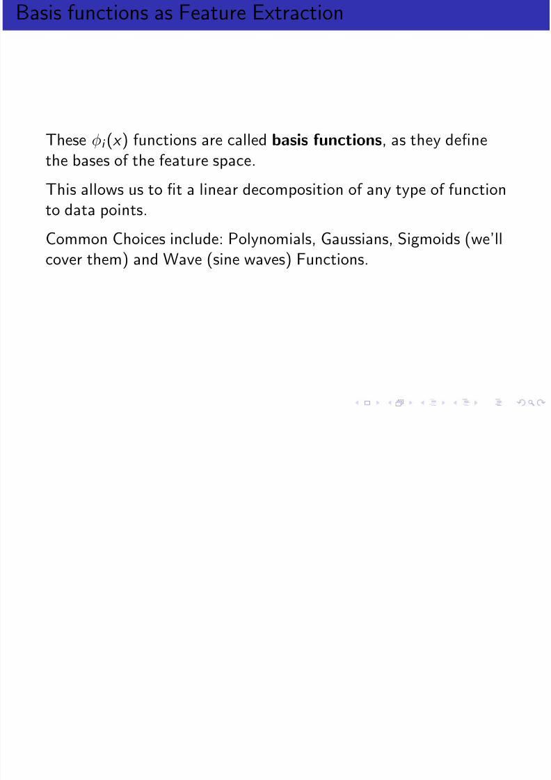
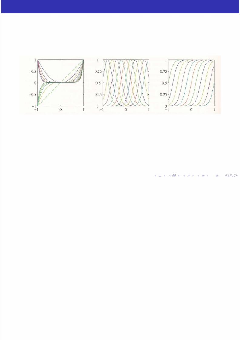
These φi (x ) functions are called basis functions, as they definethe bases of the feature space.
This allows us to fit a linear decomposition of any type of functionto data points.
Common Choices include: Polynomials, Gaussians, Sigmoids (we’llcover them) and Wave (sine waves) Functions.
8/3/2019 Andrew Rosenberg- Lecture 2.2: Linear Regression CSC 84020 - Machine Learning
http://slidepdf.com/reader/full/andrew-rosenberg-lecture-22-linear-regression-csc-84020-machine-learning 27/34
Training data v. testing data
8/3/2019 Andrew Rosenberg- Lecture 2.2: Linear Regression CSC 84020 - Machine Learning
http://slidepdf.com/reader/full/andrew-rosenberg-lecture-22-linear-regression-csc-84020-machine-learning 28/34
g g
Evaluation.
Evaluating the performance of a classifier on training data ismeaningless.
With enough parameters, a model can simply memorize(encode) every training point.
Therefore data is typically divided into two sets, training data andtesting or evaluation data.
Training data is used to learn model parameters.Testing data is used to evaluate the model.
Overfitting 1/2
8/3/2019 Andrew Rosenberg- Lecture 2.2: Linear Regression CSC 84020 - Machine Learning
http://slidepdf.com/reader/full/andrew-rosenberg-lecture-22-linear-regression-csc-84020-machine-learning 29/34
/
Overfitting 2/2
8/3/2019 Andrew Rosenberg- Lecture 2.2: Linear Regression CSC 84020 - Machine Learning
http://slidepdf.com/reader/full/andrew-rosenberg-lecture-22-linear-regression-csc-84020-machine-learning 30/34
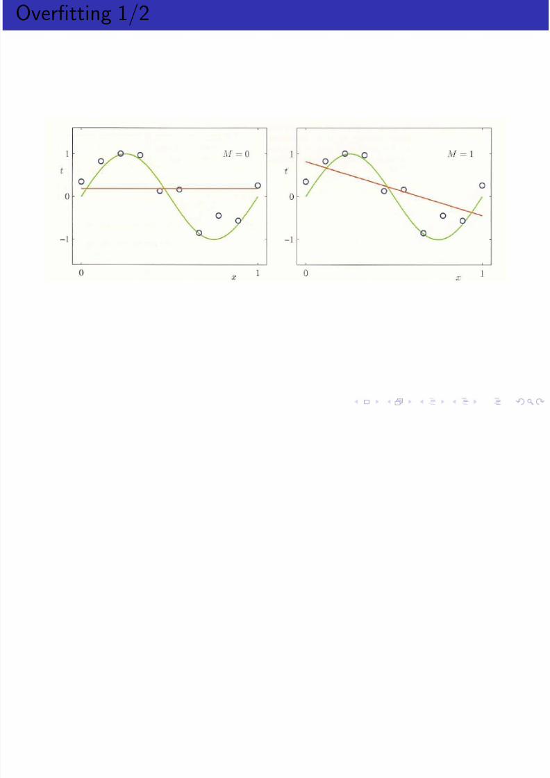
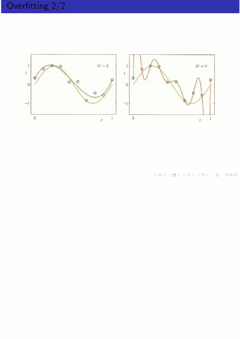
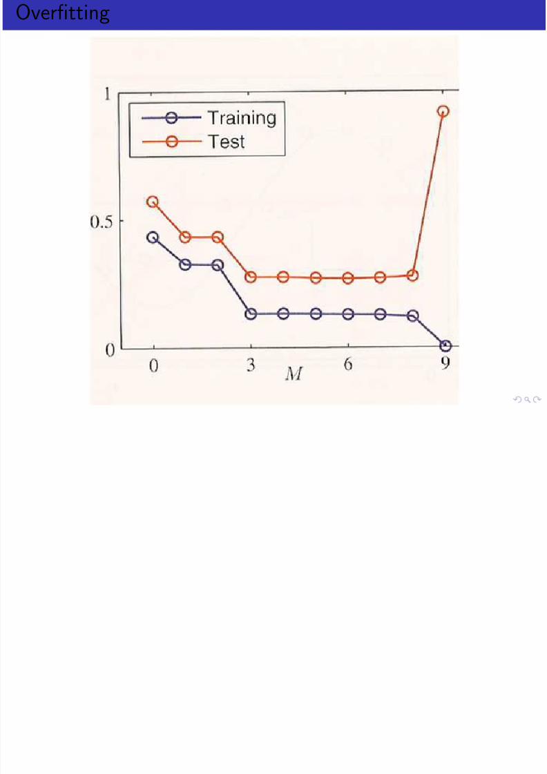
Overfitting
8/3/2019 Andrew Rosenberg- Lecture 2.2: Linear Regression CSC 84020 - Machine Learning
http://slidepdf.com/reader/full/andrew-rosenberg-lecture-22-linear-regression-csc-84020-machine-learning 31/34
What is the correct model size?
8/3/2019 Andrew Rosenberg- Lecture 2.2: Linear Regression CSC 84020 - Machine Learning
http://slidepdf.com/reader/full/andrew-rosenberg-lecture-22-linear-regression-csc-84020-machine-learning 32/34
The best model size is the size that generalizes to unseen data thebest.
We approximate this by the testing error.
One way to optimize the parameters is to minimize the testingerror.
This makes the testing data a tuning set.
However, this reduces the amount of training data in favor of parameter optimization.
Can we do this directly without sacrificing training data?
Regularization.
Context
8/3/2019 Andrew Rosenberg- Lecture 2.2: Linear Regression CSC 84020 - Machine Learning
http://slidepdf.com/reader/full/andrew-rosenberg-lecture-22-linear-regression-csc-84020-machine-learning 33/34
Who cares about Linear Regression?
It’s a simple modeling approach that learns efficiently.By extensions to the basis functions, its very extensible.
With regularization we can construct efficient models.
Bye

8/3/2019 Andrew Rosenberg- Lecture 2.2: Linear Regression CSC 84020 - Machine Learning
http://slidepdf.com/reader/full/andrew-rosenberg-lecture-22-linear-regression-csc-84020-machine-learning 34/34
Next
Regularization in Linear Regression.