Embed Size (px)
Citation preview

To the Graduate Council: I am submitting herewith a thesis written by Vivek Agarwal entitled “Ridge Regression Approach to Color Constancy”. I have examined the final electronic copy of this thesis for form and content and recommend that it be accepted in partial fulfillment of the requirements for the degree of Master of Science, with a major in Electrical Engineering. Mongi A. Abidi
__________________________
Major Professor
We have read this thesis and recommend its acceptance: Andrei V. Gribok _______________________________________
Andreas Koschan _______________________________________
Besma R. Abidi _______________________________________
Seong G. Kong _______________________________________
Accepted for the Council:
Anne Mayhew ______________________________________________________________________
Vice Chancellor and Dean of Graduate Studies
(Original signatures are on file with official student records)
Ridge Regression Approach to Color Constancy
A Thesis
Presented for the Master of Science
Degree The University of Tennessee, Knoxville
Vivek Agarwal Spring 2005

ii
Acknowledgements First and foremost, I would like to extend my appreciation towards my parents and brother who have always been instrumental in all my endeavors, for their continuous support and encouragement. Let me introduce you to my parents Mr. Vijay Krishna Agarwal, Mrs. Urmila Agarwal and brother cum friend Mr. Amit Agarwal. I would like to thank my advisor Dr. Mongi. A. Abidi for his valuable guidance, opportunities and financial support that he presented to me during my graduate master’s program at University of Tennessee, Knoxville. I am grateful to Dr. Andrei Gribok for his guidance, immense knowledge based discussion on various topics that proved instrumental towards my thesis and other research works in the lab. Knowledge and experience gained by me while working under him is immeasurable. He helped me seek focus and always got the best out of me. I thank him for all the good he has brought to my graduate education, for reviewing my thesis work, for his patience and for all the technical and non technical discussions. I am thankful to Dr. Andreas Koschan for sharing his immense knowledge in the field of color constancy research with me, reviewing my thesis, and for many other technical discussions. I would like to thank Dr. Besma Abidi for her guidance, valuable advices and for reviewing my thesis. I thank Dr. Seong. G. Kong for reviewing my thesis work. I would also like to thank Dr. David L. Page for helping me with my presentations and technical writing skills initially. Within IRIS laboratory among staff’s, I would like to thank Vicki Courtney Smith for extending friendly welcome all the time and taking care of all the essential paperwork’s. I thank Justin Acuff, for providing all the technical support in terms of computers and instrumentations used towards my research. I also thank Tak Motoyama, Sharon Foy (former employee’s of IRIS lab), and Kim Cate for all their help. Being part of a big and versatile research group, I owe thanks to my fellow graduate students. I extend sincere gratitude towards all for the resourceful conservations that helped my research, plus for providing a warm and friendly working environment. I would like to thank in particular Sangkyu Kang for all the informational conservations and for sharing his database with me. Finally, I would like to thank all my friends for all the fun time and support in all these years. Sincere thanks to all.
iii
Abstract This thesis presents the work on color constancy and its application in the field of computer vision. Color constancy is a phenomena of representing (visualizing) the reflectance properties of the scene independent of the illumination spectrum. The motivation behind this work is two folds: The primary motivation is to seek ‘consistency and stability’ in color reproduction and algorithm performance respectively because color is used as one of the important features in many computer vision applications; therefore consistency of the color features is essential for high application success. Second motivation is to reduce ‘computational complexity’ by preserving the primary motivation. This work presents machine learning approach to color constancy. An empirical model is developed from the training data. Neural network and support vector machine are two prominent learning theory algorithms. The work on support vector machine based color constancy shows its superior performance over neural networks based color constancy in terms of stability. But support vector machine is time consuming method. Alternative approach to support vector machine, is a simple, fast and analytically solvable linear modeling technique known as ‘Ridge regression’. It learns the dependency between the surface reflectance and illumination from a presented training sample of data. Ridge regression provides answer to the two fold motivation behind this work, i.e., stable and computationally simple approach. The proposed algorithms, ‘Support vector machine’ and ‘Ridge regression’ are three step process: First, an input matrix constructed from the preprocessed training data set is trained to obtain a trained model. Second, test images are presented to the trained model to obtain the chromaticity estimate of the illuminants present in the testing images. Finally, linear diagonal transformation is performed to obtain the color corrected image. The results show the effectiveness of the proposed algorithms on both calibrated and uncalibrated data set in comparison to the methods discussed in literature review. Finally, thesis concludes with a complete summary on comparison between the proposed approaches and other algorithms.
iv
Contents 1 INTRODUCTION..................................................................................................... 1
1.1 Defining Color and Color constancy .............................................................. 1 1.2 Human Vision System and Machine Vision Systems..................................... 3 1.3 Motivation....................................................................................................... 3 1.4 Proposed Approach......................................................................................... 5 1.5 Document Outline........................................................................................... 7
2 COLOR SPACES AND COLOR CONSTANCY EQUATION........................... 8 2.1 Assumptions and Pre-processing .................................................................... 8 2.2 Color constancy equations ............................................................................ 10
2.2.1 Diagonal Illumination Model............................................................ 12 2.2.2 Color constancy for non inverse gamma corrected images .............. 12
2.3 Color spaces .................................................................................................. 14 2.3.1 RGB color space ............................................................................... 14 2.3.2 Chromaticity color space .................................................................. 16 2.3.3 CIE color space................................................................................. 16
3 LITERATURE REVIEW ...................................................................................... 18 3.1 Introduction to color constancy literature ..................................................... 18 3.2 Transformation based algorithms ................................................................. 20
3.2.1 General Linear Transforms............................................................... 20 3.2.2 Diagonal Linear Transforms............................................................. 20 3.2.3 Gray World algorithm....................................................................... 21 3.2.4 Scale by max algorithm .................................................................... 22
3.3 Retinex algorithm.......................................................................................... 22 3.4 Gamut algorithms.......................................................................................... 25 3.5 Statistical color constancy algorithms .......................................................... 29
3.5.1 Bayesian algorithm ........................................................................... 29 3.5.2 Color by correlation algorithm.......................................................... 31
3.6 Learning theory based algorithms................................................................. 33 3.7 Summary....................................................................................................... 34
4 NEURAL NETWORK BASED COLOR CONSTANCY................................... 38 4.1 Single layer perceptron and Multi-layer perceptron ..................................... 38 4.2 Activation functions...................................................................................... 40 4.3 Error back propagation algorithm................................................................. 41 4.4 Neural network for color constancy.............................................................. 42
4.4.1 Bootstrapping algorithm ................................................................... 42 4.4.2 Chromaticity estimation of training data .......................................... 42 4.4.3 Training of neural network ............................................................... 43 4.4.4 Testing neural network ..................................................................... 47
4.5 Limitations of neural network....................................................................... 47 5 SUPPORT VECTOR MACHINE BASED COLOR CONSTANCY................ 50
5.1 Support Vector Machines for Regression ..................................................... 50

v
5.1.1 Loss functions ................................................................................... 51 5.1.2 Linear regression............................................................................... 53 5.1.3 Feature spaces ................................................................................... 54 5.1.4 Nonlinear regression ......................................................................... 55
5.2 Selection of free parameters.......................................................................... 56 5.3 Support Vector Regression for color constancy ........................................... 57
5.3.1 Training support vector machine ...................................................... 57 5.3.2 Testing support vector machine........................................................ 58
6 RIDGE REGRESSION BASED COLOR CONSTANCY................................. 59 6.1 Ordinary Least Squares................................................................................. 59 6.2 Ridge regression............................................................................................ 61 6.3 Cross Validation selection of
λ..................................................................... 62
6.4 Ridge regression for color constancy............................................................ 63 7 COMPARISON OF COLOR CONSTANCY ALGORITHMS ......................... 64
7.1 Algorithm performance for calibrated real images....................................... 64 7.2 Algorithm performance for uncalibrated real images................................... 83 7.3 Analysis of Algorithm performances............................................................ 90
8 CONCLUSION AND FUTURE WORK .............................................................. 96 8.1 Conclusions................................................................................................... 96 8.2 Future work................................................................................................... 97
REFERENCES.............................................................................................................. 100 APPENDIX.................................................................................................................... 109 VITA............................................................................................................................... 111

vi
List of Tables Table 3.1 Comparison of color constancy classification based on advantages and disadvantages….................................................................................................................36 Table 3.2 Comparison based on accuracy, time and practicality of each algorithm……………...37 Table 5.1 Kernel function for nonlinear support vector regression…………………….………...55 Table 7.1 Optimized values of SVM free parameters using cross validation………………….....68 Table 7.2 RMS error measures of (r, g) chromaticity space of all 321 real images using each
algorithm............................................................................................................................76
vii
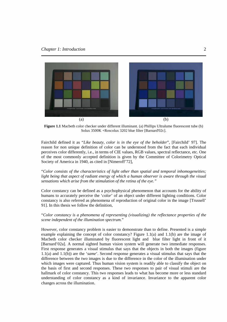
List of Figures Figure 1.1 Macbeth color checker under different illuminant..........................................................2
Figure 1.2 A graphical representation of image formation in eye....................................................3
Figure 1.3 A two consecutive frames of a scene illustrating the affect of illumination on the color
images formation.. ...................................................................................................................4
Figure 1.4 A flow chart of the proposed approach...........................................................................6
Figure 2.1 Types of surface reflection..............................................................................................9
Figure 2.2 An example showing the chromaticity shift in an image captured under different
illuminant …………………………………………………………………………………...11
Figure 2.3 The 3-dimensional schematic representation of RGB color space [Gonzalez’01]. ......15
Figure 2.4 CIE color space.............................................................................................................17
Figure 3.1 Schematic representation of classification of color constancy literature. .....................19
Figure 3.2 Gaussian distribution of the surround functions for different sigma values.. ...............24
Figure 3.3 Illustration of 3D gamut mapping algorithm [Barnard'02a]. ........................................27
Figure 3.4 The convex polygon denotes the gamut of feasible mapping calculated by 2D
perspective. The cone bounds the corresponding 3D set. The mean of the perspective gamut
of mapping (open circle) is quite different from the mean calculated in 3D (filled circle) ...28
Figure 3.5 Three steps to build correlation matrix ……………..…………………………….…..32
Figure 3.6 Three steps to solve for color constancy……………………………….......................32
Figure 4.1 Single layer perceptron. ................................................................................................39
Figure 4.2 Multilayer perceptron ...................................................................................................39
Figure 4.3 Sigmoid activation function..........................................................................................41
Figure 4.4 Plots red versus green with slices in blue whose magnitude increases from left to right.
...............................................................................................................................................43
Figure 4.5 Plots green versus blue and slices in red whose magnitude increases from left to right.
...............................................................................................................................................44
Figure 4.6. Plots red versus blue with slices in green whose magnitude increases from left to
right........................................................................................................................................45
Figure 4.7 Quantization of chromaticity space.. ............................................................................46
Figure 4.8 Neural network architecture..........................................................................................48
Figure 5.1 Loss Functions in SVM. ...............................................................................................52
viii
Figure 5.2 Concept of nonlinear support vector regression in high dimensional feature space.....54
Figure 7.1 Chromaticity distribution of the 11 illuminant sets used to generate calibrated test images ……………………………………………………….…………………………………...65
Figure 7.2 Chromaticity distribution of the training dataset of images…………………………..65
Figure 7.3 Influence of increasing the number of hidden neurons (H1) on training time………..66
Figure 7.4 A plot showing the training of the neural network of architecture 1024-10-2 to the
empirically selected performance goal of 0.0095..................................................................67
Figure 7.5 The estimated values of the chromaticities for the training dataset of images obtained
using a trained neural network of architecture 1034-10-2 .....................................................67
Figure 7.6 Cross validation curve for optimal selection of “Epsilon” for each of the individual support vector machines. (a) r – chromaticity SVM (b) g – chromaticity SVM ……………………………………...………………..…………………………………...69
Figure 7.7 Cross validation curve for optimal selection of “Sigma” for each of the individual support vector machine (a) r – chromaticity SVM (b) g – chromaticity SVM ……………………………………….……………………….…………………………..70
Figure 7.8 Cross validation curve for optimal selection of “Sigma” for each of the individual support vector machine (a) r – chromaticity SVM (b) g – chromaticity SVM ……………………………………..……………………………………………………..71
Figure 7.9 Estimated values of chromaticities of the training dataset of images obtained from
optimized nonlinear SVR ......................................................................................................72
Figure 7.10 Ridge regression optimization curve and estimated values of chromaticities. (a) Cross
validation curve for regularization parameter (lambda) and (b) Estimated values of the
chromaticities of the training dataset of images ....................................................................73
Figure 7.11 A plot showing the estimation of chromaticities of 321 test images. (a) By neural network trained model, (b) By support vector machine trained model, and (c) By ridge regression trained model………………………...………………..……………………...74
Figure 7.12 A graphical representation of algorithm performance for 321 real images for each algorithm………………………………………………………………..….……...……..76
Figure 7.13 An example showing the color correction using each algorithm on “Blocks” image ...……………………………………………………………….……………….…….…..77
Figure 7.14 An example showing the color correction using each algorithm on "Papers" image .....
………………………………………………………………………………………………79
Figure 7.15 An example showing the color correction using each algorithm on "Fruit" image ........
...............................................................................................................................................81
Figure 7.16 An image of a downtown taken at different time of a day showing the effect of llumination variation on the color appearance of the building....……………..………....84
ix
Figure 7.17 An example showing the color correction using each algorithm on “Downtown” image ……………………….............................................................................................85
Figure 7.18 An example showing the color correction using each algorithm on “Ayres Hall" image..……………….…………………………………………………………………...87
Figure 7.19 Performance of ridge regression on airport sequences ……………………………...89
Figure 7.20 A schematic illustration showing the inconsistent behavior of neural network as
network complexity increases. (a) Chromaticity estimates of training dataset for network of
architecture 1024-10-2, (b) Chromaticity estimates of testing dataset for network of
architecture 1024-10-2, (c) Chromaticity estimates of training dataset for network of
architecture 1024-40-2 and (d) Chromaticity estimates of training dataset for network of
architecture 1024-40-2...........................................................................................................92
Figure 7.21 The ‘r’ chromaticity value estimated after 100 different training trails of (a) Neural network, (b) Support vector machines, and (c) Ridge regression ……………..………...93
Figure 7.22 Prediction errors obtained after 100 different training trails of neural network, support vector regression, and ridge regression …………………………………...…….……….94
Chapter 1: Introduction
1
Chapter 1
1 INTRODUCTION This chapter presents an introduction on the concept of color constancy; its significance in machine vision system and its application in the field of computer vision. Human vision system has a unique ability to differentiate between the different colors present in the world with precise accuracy. It can also differentiate the scenes or objects based on texture, shape, density, temperature, color, complexities, and scenes or objects under different illumination properties. For instance look at figure 1.1, you are provided with two images of an object taken under different lighting conditions, say fluorescent light and red light. You are asked to identify the object and difference between the two images. What would be your response? Definitely, the response will be, “The object in two images are the same and the difference between two images is the color of light under which the images were captured.” This is because of the ability of human vision system to discount the influence of different illumination and recognize the object correctly. Human vision system exhibits has high degree of color constancy. This simple looking behavior of human vision system involves large number of sensor operations in parallel. The researchers over last few decades are working towards obtaining the same in machine vision systems. As computer vision engineers, we often wonder “How machine vision system would react given the same situation?” Can machine vision system behave analogous to human vision system? It is a million dollar question that is not easy to answer. In this thesis, we address some of the issues regarding machine vision color. Let’s begin by looking in to the multiple definition of the color and defining color constancy in section 1.1. A brief insight is provided in section 1.2 on human vision system and machine vision systems. In section 1.3 we present the motivation behind this work and scope of its application. The proposed approach is discussed in section 1.4. The outline of the thesis is presented in section 1.5.
1.1 Defining Color and Color constancy What is color? It is a simple question surprisingly with no precise answer. In most of the color research literature it is noted that ‘Color’ is not defined for reasons that question has multiple answers. A distinguished scientist Lars Sivik expressed it as follows [Sivik’97], “Blessed are the “naive”, those who do not know anything about color in a so-called scientific meaning — for them color is no problem. Color is as self-evident as most other things and phenomena in life, like night and day, up and down, air and water. And all seeing humans know what color is. It constitutes, together with form, our visual world. I have earlier used the analogy with St. Augustine’s sentence about time: “Everybody knows what time is — until you ask him to explain what it is.” It is the same with color.”
Chapter 1: Introduction
2
(a) (b)
Figure 1.1 Macbeth color checker under different illuminant. (a) Phillips Ultralume fluorescent tube (b) Solux 3500K +Roscolux 3202 blue filter [Barnard'02c].
Fairchild defined it as “Like beauty, color is in the eye of the beholder”, [Fairchild’ 97]. The reason for non unique definition of color can be understood from the fact that each individual perceives color differently, i.e., in terms of CIE values, RGB values, spectral reflectance, etc. One of the most commonly accepted definition is given by the Committee of Colorimetry Optical Society of America in 1940, as cited in [Nimeroff’72], “Color consists of the characteristics of light other than spatial and temporal inhomogeneities; light being that aspect of radiant energy of which a human observer is aware through the visual sensations which arise from the stimulation of the retina of the eye.” Color constancy can be defined as a psychophysical phenomenon that accounts for the ability of humans to accurately perceive the ‘color’ of an object under different lighting conditions. Color constancy is also referred as phenomena of reproduction of original color in the image [Trussell’ 91]. In this thesis we follow the definition, “Color constancy is a phenomena of representing (visualizing) the reflectance properties of the scene independent of the illumination spectrum.” However, color constancy problem is easier to demonstrate than to define. Presented is a simple example explaining the concept of color constancy? Figure 1.1(a) and 1.1(b) are the image of Macbeth color checker illuminated by fluorescent light and blue filter light in front of it [Barnard’02a]. A normal sighted human vision system will generate two immediate responses. First response generates a visual stimulus that says that the objects in both the images (figure 1.1(a) and 1.1(b)) are the ‘same’. Second response generates a visual stimulus that says that the difference between the two images is due to the difference in the color of the illumination under which images were captured. Thus human vision system is readily able to classify the object on the basis of first and second responses. These two responses to pair of visual stimuli are the hallmark of color constancy. This two responses leads to what has become more or less standard understanding of color constancy as a kind of invariance. Invariance to the apparent color changes across the illumination.
Chapter 1: Introduction
3
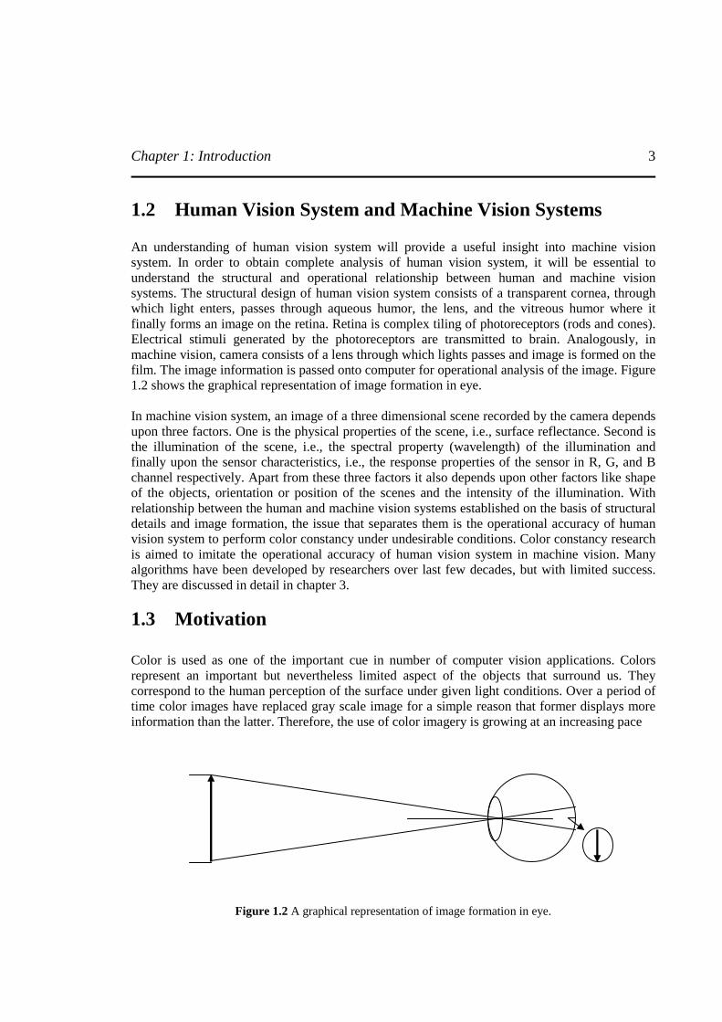
1.2 Human Vision System and Machine Vision Systems An understanding of human vision system will provide a useful insight into machine vision system. In order to obtain complete analysis of human vision system, it will be essential to understand the structural and operational relationship between human and machine vision systems. The structural design of human vision system consists of a transparent cornea, through which light enters, passes through aqueous humor, the lens, and the vitreous humor where it finally forms an image on the retina. Retina is complex tiling of photoreceptors (rods and cones). Electrical stimuli generated by the photoreceptors are transmitted to brain. Analogously, in machine vision, camera consists of a lens through which lights passes and image is formed on the film. The image information is passed onto computer for operational analysis of the image. Figure 1.2 shows the graphical representation of image formation in eye. In machine vision system, an image of a three dimensional scene recorded by the camera depends upon three factors. One is the physical properties of the scene, i.e., surface reflectance. Second is the illumination of the scene, i.e., the spectral property (wavelength) of the illumination and finally upon the sensor characteristics, i.e., the response properties of the sensor in R, G, and B channel respectively. Apart from these three factors it also depends upon other factors like shape of the objects, orientation or position of the scenes and the intensity of the illumination. With relationship between the human and machine vision systems established on the basis of structural details and image formation, the issue that separates them is the operational accuracy of human vision system to perform color constancy under undesirable conditions. Color constancy research is aimed to imitate the operational accuracy of human vision system in machine vision. Many algorithms have been developed by researchers over last few decades, but with limited success. They are discussed in detail in chapter 3.
1.3 Motivation
Color is used as one of the important cue in number of computer vision applications. Colors represent an important but nevertheless limited aspect of the objects that surround us. They correspond to the human perception of the surface under given light conditions. Over a period of time color images have replaced gray scale image for a simple reason that former displays more information than the latter. Therefore, the use of color imagery is growing at an increasing pace
Figure 1.2 A graphical representation of image formation in eye.
Chapter 1: Introduction
4
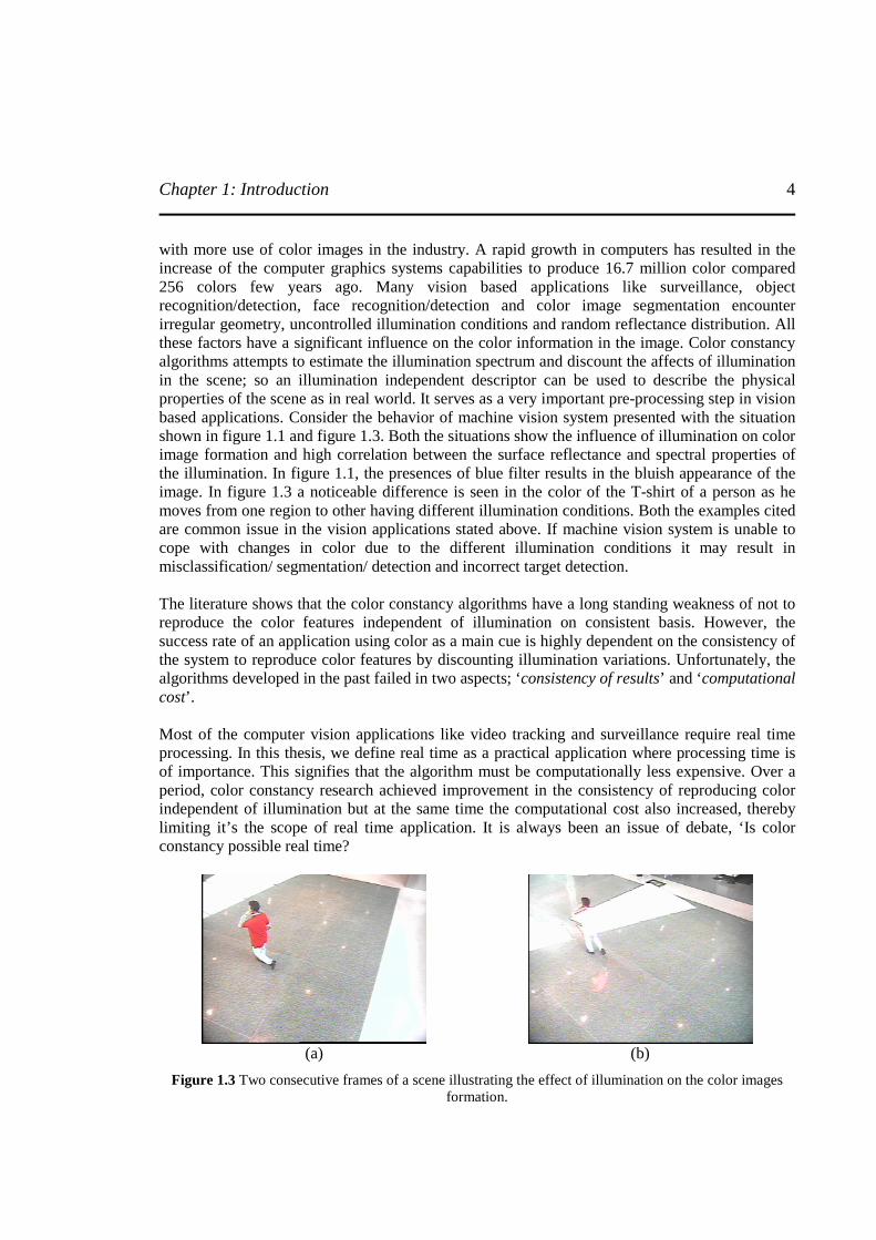
with more use of color images in the industry. A rapid growth in computers has resulted in the increase of the computer graphics systems capabilities to produce 16.7 million color compared 256 colors few years ago. Many vision based applications like surveillance, object recognition/detection, face recognition/detection and color image segmentation encounter irregular geometry, uncontrolled illumination conditions and random reflectance distribution. All these factors have a significant influence on the color information in the image. Color constancy algorithms attempts to estimate the illumination spectrum and discount the affects of illumination in the scene; so an illumination independent descriptor can be used to describe the physical properties of the scene as in real world. It serves as a very important pre-processing step in vision based applications. Consider the behavior of machine vision system presented with the situation shown in figure 1.1 and figure 1.3. Both the situations show the influence of illumination on color image formation and high correlation between the surface reflectance and spectral properties of the illumination. In figure 1.1, the presences of blue filter results in the bluish appearance of the image. In figure 1.3 a noticeable difference is seen in the color of the T-shirt of a person as he moves from one region to other having different illumination conditions. Both the examples cited are common issue in the vision applications stated above. If machine vision system is unable to cope with changes in color due to the different illumination conditions it may result in misclassification/ segmentation/ detection and incorrect target detection. The literature shows that the color constancy algorithms have a long standing weakness of not to reproduce the color features independent of illumination on consistent basis. However, the success rate of an application using color as a main cue is highly dependent on the consistency of the system to reproduce color features by discounting illumination variations. Unfortunately, the algorithms developed in the past failed in two aspects; ‘consistency of results’ and ‘computational cost’. Most of the computer vision applications like video tracking and surveillance require real time processing. In this thesis, we define real time as a practical application where processing time is of importance. This signifies that the algorithm must be computationally less expensive. Over a period, color constancy research achieved improvement in the consistency of reproducing color independent of illumination but at the same time the computational cost also increased, thereby limiting it’s the scope of real time application. It is always been an issue of debate, ‘Is color constancy possible real time?
(a) (b)
Figure 1.3 Two consecutive frames of a scene illustrating the effect of illumination on the color images formation.
Chapter 1: Introduction
5
All these concerns and questions present motivation towards the work in this thesis. The motivation behind this work is two folds; primarily to develop a color constancy algorithm that ensures better reproduction of color independent of illumination. Stability of the algorithms and consistency of results are the key issues. Second motivation is to reduce the computational complexity and computational cost of the proposed color constancy algorithm suitable for real time applications by not violating the primary motivation. Success in achieving both motivation will enable to widen the scope of application of the color constancy algorithms in computer vision applications. Color constancy algorithm can be applied for real time applications like face detection, video surveillance, target detection. All these applications ask for consistency and low computational cost. On the other hand, in the case of applications like color image segmentation, object recognition where computational cost is a minor issue when compared to consistency of the result, color constancy algorithm will be able to satisfy the need of those applications too. With all these issues in consideration, we propose two learning theory based methods in next subsection 1.4.
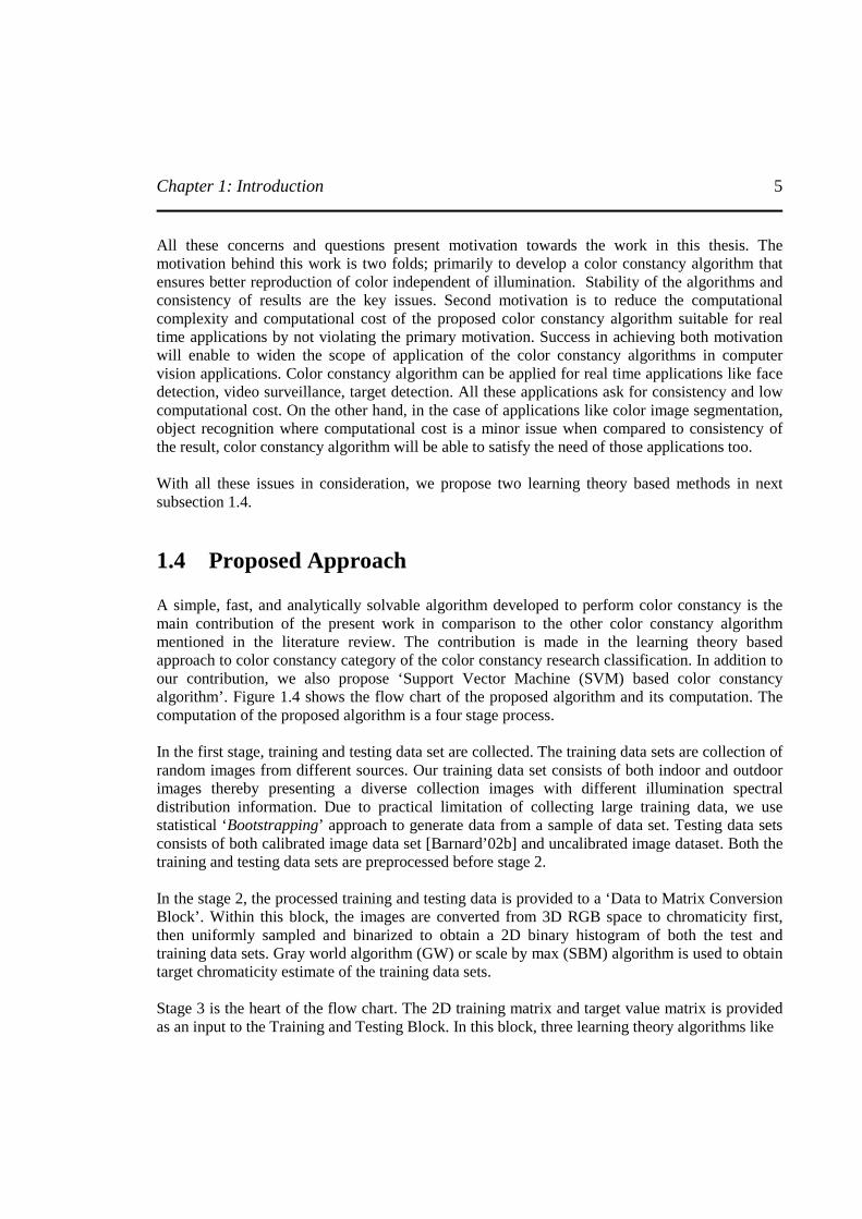
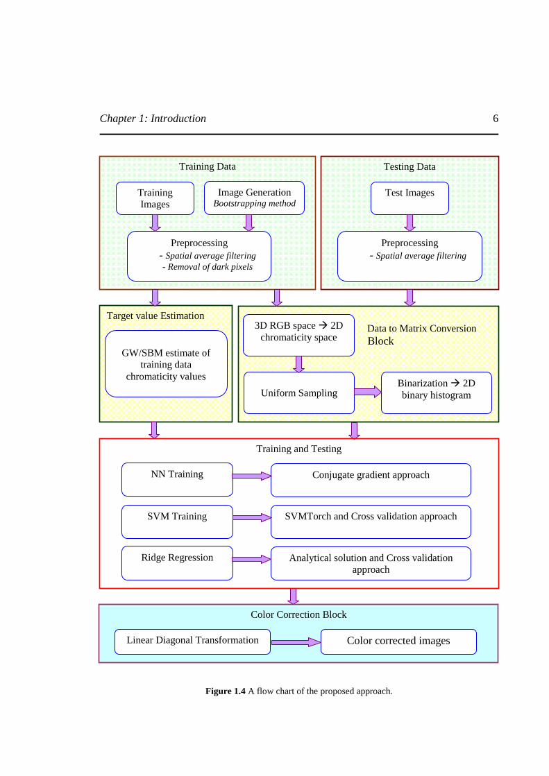
1.4 Proposed Approach A simple, fast, and analytically solvable algorithm developed to perform color constancy is the main contribution of the present work in comparison to the other color constancy algorithm mentioned in the literature review. The contribution is made in the learning theory based approach to color constancy category of the color constancy research classification. In addition to our contribution, we also propose ‘Support Vector Machine (SVM) based color constancy algorithm’. Figure 1.4 shows the flow chart of the proposed algorithm and its computation. The computation of the proposed algorithm is a four stage process. In the first stage, training and testing data set are collected. The training data sets are collection of random images from different sources. Our training data set consists of both indoor and outdoor images thereby presenting a diverse collection images with different illumination spectral distribution information. Due to practical limitation of collecting large training data, we use statistical ‘Bootstrapping’ approach to generate data from a sample of data set. Testing data sets consists of both calibrated image data set [Barnard’02b] and uncalibrated image dataset. Both the training and testing data sets are preprocessed before stage 2. In the stage 2, the processed training and testing data is provided to a ‘Data to Matrix Conversion Block’. Within this block, the images are converted from 3D RGB space to chromaticity first, then uniformly sampled and binarized to obtain a 2D binary histogram of both the test and training data sets. Gray world algorithm (GW) or scale by max (SBM) algorithm is used to obtain target chromaticity estimate of the training data sets. Stage 3 is the heart of the flow chart. The 2D training matrix and target value matrix is provided as an input to the Training and Testing Block. In this block, three learning theory algorithms like
Chapter 1: Introduction
6
Figure 1.4 A flow chart of the proposed approach.
Testing Data
Data to Matrix Conversion Block
Training Data
3D RGB space � 2D chromaticity space
Uniform Sampling
Binarization � 2D binary histogram
Target value Estimation
GW/SBM estimate of
training data chromaticity values
Color Correction Block
NN Training
SVM Training
Analytical solution and Cross validation approach
Conjugate gradient approach
Ridge Regression
SVMTorch and Cross validation approach
Linear Diagonal Transformation Color corrected images
Training Images
Image Generation Bootstrapping method Image Generation
Preprocessing - Spatial average filtering - Removal of dark pixels
Test Images
Preprocessing - Spatial average filtering
Training and Testing
Chapter 1: Introduction
7
Neural network (NN), SVM and ridge regression are trained. NN is trained using Bayesian regularization. SVM is trained using SVMTorch algorithm and the free parameters are optimized using cross validation. Ridge regression is solved analytically and the free parameter is optimized using cross validation. To these trained models, 2D testing matrix is provided as input, to obtain the estimate of the chromaticity values for the test images. Finally, in the stage 4, the estimated chromaticity values are provided to ‘Color Correction Block’. Linear diagonal transformation algorithm is used to obtain the diagonal model. The test images are corrected as per diagonal model to obtain color corrected images.
1.5 Document Outline The thesis is outlined as follows: The chapter 2 talks about assumptions, pre-processing steps, color spaces, and basic color constancy equations applied in color constancy research. Following chapter 2, in chapter 3 state of the art of color constancy research is described. This chapter is a comprehensive literature review on the various color constancy algorithms and their classifications. A comparison is provided at the end of the chapter. In chapter 4, neural network based color constancy is presented. Different aspects regarding training and testing the network in estimating illuminant chromaticity is present in a detailed discussion. In chapter 5, support vector machine based color constancy; one of our proposed algorithms is presented. Issues related to training and testing support vector machines are discussed. In chapter 6, ridge regression based color constancy; another of our proposed algorithms is presented. Analytical solution of the proposed approach is presented in the chapter showing its effectiveness over other algorithms. Chapter 7 contains results obtained by both quantitatively and qualitative (visual) analysis of the results obtained from proposed algorithms and other algorithms in the literature. The results are obtained for both calibrated and non calibrated data sets. Finally, in chapter 8, conclusion is drawn on the work with discussion on the possible future extension of the work.
Chapter 2: Color spaces and color constancy equations
8
Chapter 2
2 COLOR SPACES AND COLOR CONSTANCY EQUATION In this chapter, mathematical formulation on the basic theories associated with color constancy and brief explanation on different color spaces is presented. This analysis provides a good insight towards proper understanding of literature. Also discussed are the various assumptions and their significance on color constancy research. There are number of factors that influence the assumptions. In the following subsections, you will be apprised with the affects of all these factors. In past few decades, number of color spaces has been developed to represent colors. Discussing all the color spaces in detail is beyond the scope of this thesis. Therefore emphasis is paid on the most commonly used color spaces such as RGB and CIELAB in color constancy research. Other prominent color spaces that are not discussed here like HSV, HSI, YCrCb, YIQ, and YUV can be obtained from the linear and nonlinear transformation of RGB color space. The subsection 2.1 discusses the assumptions and preprocessing taken into consideration in color constancy literature. The subsection 2.2 presents simple basic color constancy notations. The subsection 2.3 talks about the color spaces.
2.1 Assumptions and Pre-processing Color image is a function of ),,( λyxS the surface reflectance, )(λI the illumination condition of
the scene, and the )(λk
C sensor characteristics as a function of the wavelength of the incident
light λ , over a visible spectrumω is represented in the equation (2.1).
λω
λλλ dk
CIyxSyxk
)()(),,(),(I ∫= (2.1)
where yx and are the pixels location in an image; the subscript k represents the sensors response
in kth channel and ),(I yxk
is the image corresponding to the kth channel (k = 3). The color
cameras have 3 channels responses. In rest of the document, all three channels will be represented as R, G, and B corresponding to red, green and blue channel response respectively. Factors such as back current, auto iris, white balancing, gamma correction, blooming affect and underexposures are the examples of sensor factors. In practical situation no two sensors will have similar characteristics; therefore careful calibration of sensor is essential. Homogeneous lighting and inhomogeneous lighting conditions accounts for the illumination factors. A scene with
Chapter 2: Color spaces and color constancy equations
9
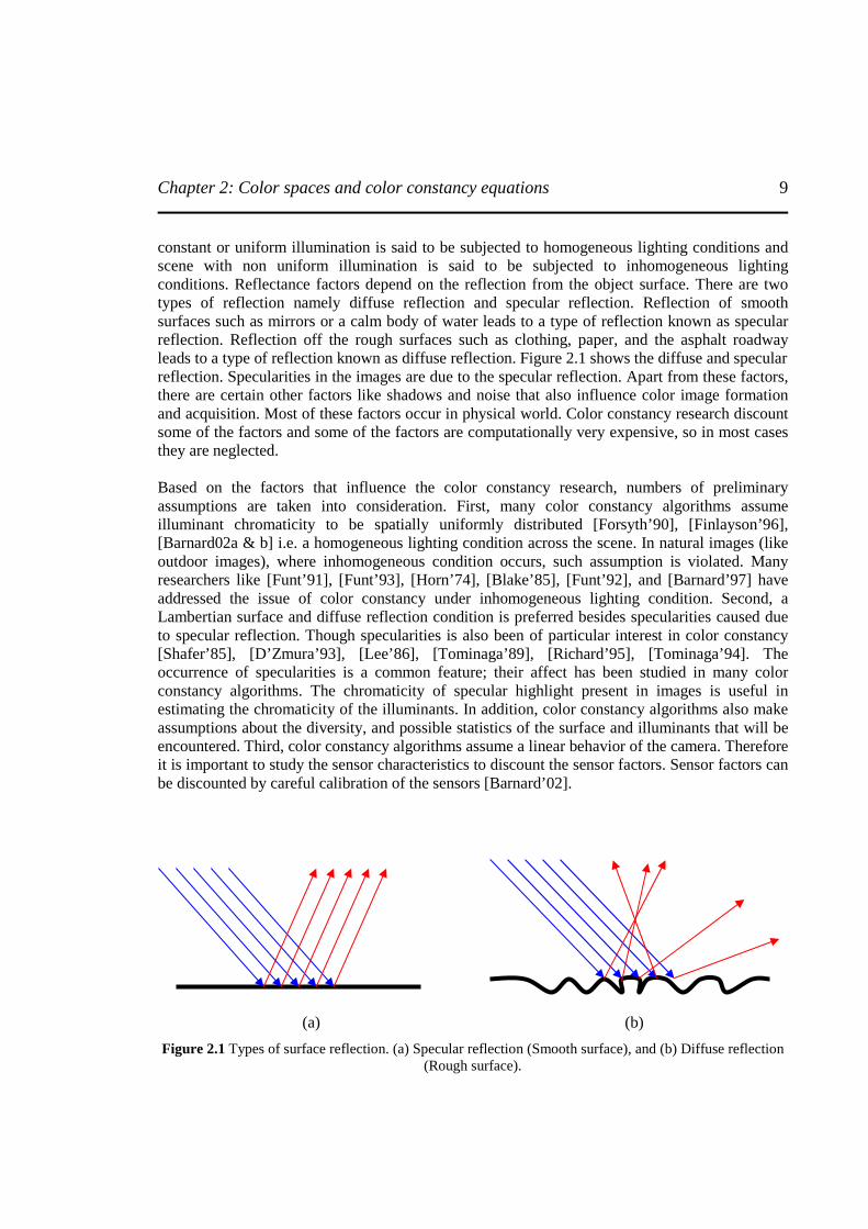
constant or uniform illumination is said to be subjected to homogeneous lighting conditions and scene with non uniform illumination is said to be subjected to inhomogeneous lighting conditions. Reflectance factors depend on the reflection from the object surface. There are two types of reflection namely diffuse reflection and specular reflection. Reflection of smooth surfaces such as mirrors or a calm body of water leads to a type of reflection known as specular reflection. Reflection off the rough surfaces such as clothing, paper, and the asphalt roadway leads to a type of reflection known as diffuse reflection. Figure 2.1 shows the diffuse and specular reflection. Specularities in the images are due to the specular reflection. Apart from these factors, there are certain other factors like shadows and noise that also influence color image formation and acquisition. Most of these factors occur in physical world. Color constancy research discount some of the factors and some of the factors are computationally very expensive, so in most cases they are neglected. Based on the factors that influence the color constancy research, numbers of preliminary assumptions are taken into consideration. First, many color constancy algorithms assume illuminant chromaticity to be spatially uniformly distributed [Forsyth’90], [Finlayson’96], [Barnard02a & b] i.e. a homogeneous lighting condition across the scene. In natural images (like outdoor images), where inhomogeneous condition occurs, such assumption is violated. Many researchers like [Funt’91], [Funt’93], [Horn’74], [Blake’85], [Funt’92], and [Barnard’97] have addressed the issue of color constancy under inhomogeneous lighting condition. Second, a Lambertian surface and diffuse reflection condition is preferred besides specularities caused due to specular reflection. Though specularities is also been of particular interest in color constancy [Shafer’85], [D’Zmura’93], [Lee’86], [Tominaga’89], [Richard’95], [Tominaga’94]. The occurrence of specularities is a common feature; their affect has been studied in many color constancy algorithms. The chromaticity of specular highlight present in images is useful in estimating the chromaticity of the illuminants. In addition, color constancy algorithms also make assumptions about the diversity, and possible statistics of the surface and illuminants that will be encountered. Third, color constancy algorithms assume a linear behavior of the camera. Therefore it is important to study the sensor characteristics to discount the sensor factors. Sensor factors can be discounted by careful calibration of the sensors [Barnard’02].
(a) (b)
Figure 2.1 Types of surface reflection. (a) Specular reflection (Smooth surface), and (b) Diffuse reflection (Rough surface).
Chapter 2: Color spaces and color constancy equations
10
One of the important sensor factors that needs to be corrected in to perform inverse gamma correction. Some of the researchers use appropriate method from literature [Farid’01] to estimate the value of gamma for a particular camera and perform inverse gamma correction. But color constancy algorithms are also tested on nonlinear images. In subsection 2.2, mathematical formulation is provided to show how the gamma and color constancy operation is commuted [Cardei’00]. To increase the robustness of the color constancy algorithms, preprocessing is performed on the images as in [Barnard’02b]. The first pre-processing step involves reduction of noise present in the images. In general spatial averaging on the images using a specific window size is performed [Barnard’02a], [Barnard’02b], [Rosenberg’03] to reduce the noise level. Second pre-processing step is removing dark pixels which because of noise or quantization effects do not contain reliable color information. Therefore pixels whose values are less than a given threshold are excluded from the computation. In this thesis, pixels whose value is less than 7 (0-255 scale) is neglected.
2.2 Color constancy equations Color image being a function of surface reflectance, the illumination condition of the scene, and the sensor characteristics as represented in the equation (2.1). Equation (2.2) can be obtained from equation (2.1), if both the sensor characteristics and the surface reflectance are constant, only the illumination varies, then image is solely the function (f) of illumination of the scene. This is a linear model [Brainard’97].
))((),(I λIfyxk
= (2.2)
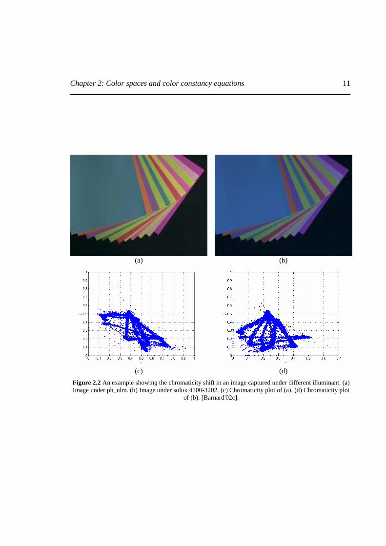
Figure 2.2 shows the yet another example of influence of illumination color on the image color. A graphical representation is also shown to illustrate the shift in the chromaticity of the same image taken under two different illuminations (Philips Ultralume Fluorescent (ph_ulm) and Solux 4100K + Roscolux 3202). The plot is obtained in the chromaticity coordinate. Thereby reiterating the objective of color constancy: to make the image formation as independent as possible of the chromaticity of the illuminant. Many theories have been suggested to solve for color constancy (see chapter 3) and most of the theories are based on the framework of linear illumination model, known as ‘Diagonal Illumination Model’. The model maps the image under one illuminant (unknown source) to the image under another illuminant (standard source) by scaling the each channel of the sensors response independently.
Chapter 2: Color spaces and color constancy equations
11
(a) (b)
(c) (d)
Figure 2.2 An example showing the chromaticity shift in an image captured under different illuminant. (a) Image under ph_ulm. (b) Image under solux 4100-3202. (c) Chromaticity plot of (a). (d) Chromaticity plot
of (b). [Barnard'02c].

Chapter 2: Color spaces and color constancy equations
12
2.2.1 Diagonal Illumination Model The diagonal illumination model is a simple linear transformation model, used to obtain approximate color constancy. Finlayson [Finlayson’93], [Finlayson’94b] showed that in diagonal model using only 3 parameters is sufficient to obtain good approximate color constancy over other transformation model using 9 parameters. The efficiency of diagonal model is largely dependent on the vision system sensors. However, the diagonal model error can be reduced by performing sensor sharpening [Finlayson’94a], [Barnard’01]. Researchers [Barnard’02a], [Barnard’02b], [Finlayson’01], [Rosenberg’03] utilized a diagonal illumination model which maps the images taken under one illuminant to the images taken under another illuminant (canonical illuminant). For example, consider two images A and B taken under unknown and canonical illuminant respectively. Let AAA BGR ,, and BBB BGR ,, be the channel response of
both the images. The diagonal matrix (D ) corresponding to diagonal illumination model is given in equation (2.3) and (2.4). The response of the image under unknown illuminant is mapped to the canonical illuminant by scaling the three channels using the diagonal matrix.
BDA =⋅ (2.3)
=
AB
AB
AB
BB
GG
RR
D
00
00
00
(2.4)
In some literature, the third channel which corresponds to the intensity value in the image is neglected since the interest lies in obtaining the chromaticity of the illuminant. The chromaticity co-ordinates (r, g) are computed. This reduces the 3D approach to 2D. There are number of color constancy approaches developed in chromaticity color space [Finlayson’01], [Finlayson’96], [Barnard’97], [Cardei’00]. Those algorithms make use of diagonal model in 2D space.
2.2.2 Color constancy for non inverse gamma corrected images Color constancy algorithms strictly assume a linear response of the sensors. Color correction of linear images by using the diagonal transformation method described above. V. Cardei in [Cardei’00] proved that the above equations are also valid for non inverse gamma corrected data sets, i.e. nonlinear images. Gamma correction performed by the sensors introduces nonlinearity. In [Cardei’00] it is proved that gamma correction γ and color constancy process (c ) can be commuted. Equation (2.5) shows the gamma operation on image (I) and equation (2.6) shows the color constancy process at constant gamma.
( ) γII =Γ
(2.5)
( ) DDc ⋅= I,I (2.6)
If both the process is commutable, then

Chapter 2: Color spaces and color constancy equations
13
( )( ) ( )( )DcDc ,I,I Γ=Γ (2.7)
Applying γ affects the image chromaticities so a color constancy algorithm will receive different set of input chromaticities, depending on whether or not the image has had γ applied. Moreover,
the diagonal color constancy transformation needs to be different. If ( www BGR ,, ) is the color of
known illuminant for image I and ( BGR ,, ) is an arbitrary pixels in I, then
[ ]( )( ) [ ]( ) [ ]γγ
γγ
γγγ
γγγγ BmGmRmDBGRcDBGRc BGR ,, , ,, , ,, ==Γ (2.8)
Where γD the transformation matrix with γ applied.
=B
G
R
m
m
m
D
γ
γ
γ
γ
00
00
00
(2.9)
Under known illuminant, γD is computed using the equation (2.10)
[ ]( )( ) [ ]( ) [ ] [ ]1,1,1,, , ,, , ,, ===Γ γ
γγ
γγ
γγγγγ
γ wB
wG
wR
wwwwww BmGmRmDBGRcDBGRc (2.10)
Thus the transformation matrix is given by equation (2.11),
=γ
γ
γ
γ
w
w
w
B
G
R
D
100
010
001
(2.11)
The equation (2.6) can be rewritten as a function of ( www BGR ,, ) and ( BGR ,, ).
[ ]( )( ) [ ]
⋅⋅⋅==Γ γ
γγ
γγ
γγ
γγ
γγ
γγ BB
GG
RR
BmGmRmDBGRcwww
BGR 1,
1,
1,, , ,,
(2.12)
The right hand side of equation (2.7) can be written as
( )( ) [ ]( ) ,, ,I BmGmRmDc BGRΓ=Γ (2.13)
The transformation matrix with no γ applied is
Chapter 2: Color spaces and color constancy equations
14
=
w
w
w
B
G
R
D
100
010
001
γ
(2.14)
Thus equation (2.13) becomes
[ ]( )( )
⋅⋅⋅=
⋅⋅⋅=Γ γ
γγ
γγ
γ BB
GG
RR
BB
GG
RR
DBGRcwwwwww
1,
1,
11,
1,
1 , ,,
(2.15)
Thus equation (2.12) and (2.15) shows that (2.7) is true for any pixel in image I, i.e. color constancy and γ application are commutative. Thus color constancy can be performed on nonlinear images in the same ways as on linear images. However above equation is based on the assumption of a perfect white surface in an image I. Gamma γ not only affects the chromaticities of the pixels in the image but also affect their statistical distribution because γ has a general tendency to desaturate colors. This change in the distribution of the chromaticities can adversely affect the color constancy algorithms that rely on a prior knowledge about the statistics of the world.
2.3 Color spaces Color spaces are used to describe color in color research. Number of color spaces has been developed over a period of time with unique features to describe different properties of color but we will limit ourselves to the discussion of RGB, ‘rg’ chromaticity color space and CIELAB color spaces because most of the color constancy algorithms uses only these color spaces.
2.3.1 RGB color space Red, green and blue components can be represented by the values of the scene obtained through three separate filters which is based on following equations:
∫=ω
λλλ dr
CRR )()(
(2.16)
∫=ω
λλλ dg
CRG )()(
(2.17)
∫=ω
λλλ db
CRB )()(
(2.18)
Chapter 2: Color spaces and color constancy equations
15
Where )(λrC , )(λgC , )(λbC are the color filters on the incoming light, )(λR is the radiance and λ
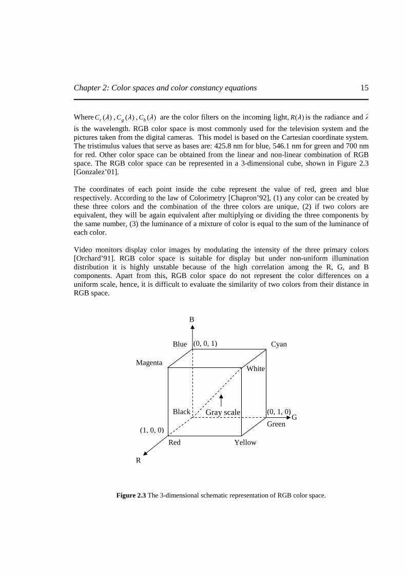
is the wavelength. RGB color space is most commonly used for the television system and the pictures taken from the digital cameras. This model is based on the Cartesian coordinate system. The tristimulus values that serve as bases are: 425.8 nm for blue, 546.1 nm for green and 700 nm for red. Other color space can be obtained from the linear and non-linear combination of RGB space. The RGB color space can be represented in a 3-dimensional cube, shown in Figure 2.3 [Gonzalez’01]. The coordinates of each point inside the cube represent the value of red, green and blue respectively. According to the law of Colorimetry [Chapron’92], (1) any color can be created by these three colors and the combination of the three colors are unique, (2) if two colors are equivalent, they will be again equivalent after multiplying or dividing the three components by the same number, (3) the luminance of a mixture of color is equal to the sum of the luminance of each color. Video monitors display color images by modulating the intensity of the three primary colors [Orchard’91]. RGB color space is suitable for display but under non-uniform illumination distribution it is highly unstable because of the high correlation among the R, G, and B components. Apart from this, RGB color space do not represent the color differences on a uniform scale, hence, it is difficult to evaluate the similarity of two colors from their distance in RGB space.
G
Figure 2.3 The 3-dimensional schematic representation of RGB color space.
Red
Magenta
Blue Cyan
White
Black
Green G
R
B
(0, 0, 1)
(0, 1, 0)
(1, 0, 0)
Yellow
Gray scale
Chapter 2: Color spaces and color constancy equations
16
2.3.2 Chromaticity color space In many color constancy applications, estimation of the brightness is not as important as estimation of color. Therefore the brightness information is ignored. This is achieved by projecting the 3D RGB color space to 2D chromaticity space. The general idea is to normalize to two color spaces, with third color space can be recovered from the other two. Equation (2.19) and (2.20) shows the normalization of R, G, B color space in to ‘rg’ chromaticity color space. The b coordinate is given by grb −−=1 .
( )BGRRr ++=
(2.19)
( )BGRGg ++= (2.20)
Finlayson [Finalyson’95], [Finlayson’94b] built a new chromaticity space based on projection rule which is given as bggbrr /,/ == . However, in some cases logarithmic chromaticity space is used. The logarithmic chromaticity space is given by equation (2.21) and (2.22).
( )rr log=′
(2.21)
( )gg log=′ (2.22)
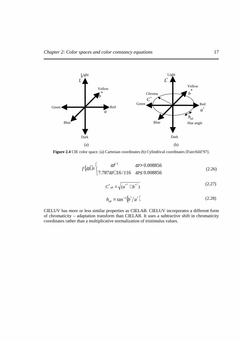
2.3.3 CIE color space CIE (Commission International de l’Eclairage) recommended two color spaces namely CIELAB and CIELUV in early 1970’s. In early 1990’s CIE adapted CIELAB as a single color space for color - difference measurement. CIELAB was developed as a color space to be used for the specification of color differences. CIE coordinates are obtained from the nonlinear transformation of the XYZ tristimulus values which in turn are obtained from the linear transformation of the RGB values. The mathematical formulation for CIELAB color space is given in equations (2.23-2.26). These equations are obtained from the cartesian representation of the CIELAB color space shown in figure 2.4 (a). The CIELAB color space can also be represented in terms of cylindrical coordinates as shown in figure 2.4(b). The limitation of the CIE space is the singularities of values due to nonlinear transformation.
The cylindrical coordinate system provides information of chroma ( *C ) and hue (hue angle in degrees) as expressed in equations (2.27) and (2.28).
( ) 16116 −=∗nYYfL
(2.23)
( ) ( )[ ]nN YYfXXfa −=∗ 500
(2.24)
( ) ( )[ ]nn ZZfYYfb −=∗ 200
(2.25)
Chapter 2: Color spaces and color constancy equations
17
∗
L
∗
a
(a) (b)
Figure 2.4 CIE color space. (a) Cartesian coordinates (b) Cylindrical coordinates [Fairchild’97].
( )
≤+>
=008856.0116/16787.7
008856.03/1
ωωωωωf
(2.26)
)(22 ∗∗∗ += baC ab
(2.27)
( )∗∗−= abhab1tan (2.28)
CIELUV has more or less similar properties as CIELAB. CIELUV incorporates a different form of chromaticity – adaptation transform than CIELAB. It uses a subtractive shift in chromaticity coordinates rather than a multiplicative normalization of tristimulus values.
Yellow ∗
b
Red *a
Blue
Green
Chroma *C
abh
Hue angle
Dark
Light
Red Green
Yellow ∗
b
Blue
Light *L
Dark
Chapter 3: Literature review
18
Chapter 3
3 LITERATURE REVIEW This chapter focuses on the state of the art of color constancy research performed in the past. Over last two decades, the color has become an active field of research because of the increase in the use of color images in industry. Color is used as an important cue in many color based applications like segmentation, object recognition, video tracking, face detection, etc. Due to versatility of applications of color constancy research, various aspects are taken into consideration while drafting down a review on color constancy research. The introduction to color constancy research is discussed in subsection 3.1. Through subsection 3.2, to 3.6, a review and analysis on different color constancy algorithms is presented. Finally, a summary is provided in subsection 3.7.
Central to solving color constancy problem is to obtain an estimate of the scene illuminant taking into consideration most of the factors discussed in chapter 2. The idea to obtain color constancy is based on many theories proposed by authors [Brainard’97], [Buchsbaum’80], [D’Zmura’94], [D’Zmura’93], [Finlayson’96], [Forsyth’90], [Land’77], [Maloney’86a], [Shafer’85], [Tominaga’96], [Finlayson’01], [Cardei’97a], [Funt’93]. Most of the theories identified color constancy as very difficult problem to solve. Therefore many researchers for simplicity considered two dimensional world of objects that are flat, matte, Lambertain surface, and uniformly illumination. All the theories also identify color constancy as an under-constrained problem i.e. an ill-posed problem. According to Hadmard, a French mathematician a problem is well posed if following three conditions are satisfied, (1) there exits a solution, (2) this solution is unique and (3) this unique solution is stable. If any one of the conditions fails then the problem is said to be ill-posed. Color constancy research has shown that it violates condition (2) and (3) of well-posedness. The past theories have shown that there exists a solution but the uniqueness and stability of the solution is not defined. The possible reason could be because of the high correlation between the colors in the image and the chromaticity (color) of the illuminant. In other words the object color and illuminant color are not uniquely separable. The significance of degree of correlation can be understood from the figures in chapter 1. Literatures review show that works have been performed to study the correlation. From early 1980’s to present, number of color constancy algorithms have been developed to discount the affect of illumination under supervised or unsupervised illumination conditions. Most of the constancy research work in early 1980’s act as foundation for most of the active color constancy research and serve as a benchmark. Some of the early color constancy algorithms includes gray world algorithm [Buchsbaum’80], scale by max algorithm, Von Kries color
3.1 Introduction to color constancy literature
Chapter 3: Literature review
19
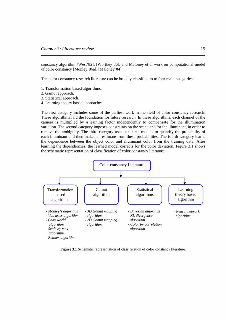
constancy algorithm [West’82], [Worthey’86], and Maloney et al work on computational model of color constancy [Monley’86a], [Maloney’84]. The color constancy research literature can be broadly classified in to four main categories: 1. Transformation based algorithms. 2. Gamut approach. 3. Statistical approach. 4. Learning theory based approaches. The first category includes some of the earliest work in the field of color constancy research. These algorithms laid the foundation for future research. In these algorithms, each channel of the camera is multiplied by a gaining factor independently to compensate for the illumination variation. The second category imposes constraints on the scene and /or the illuminant, in order to remove the ambiguity. The third category uses statistical models to quantify the probability of each illuminant and then makes an estimate from these probabilities. The fourth category learns the dependence between the object color and illuminant color from the training data. After learning the dependencies, the learned model corrects for the color deviation. Figure 3.1 shows the schematic representation of classification of color constancy literature.
Figure 3.1 Schematic representation of classification of color constancy literature.
Color constancy Literature
Transformation based
algorithms
Gamut algorithm
Statistical algorithms
Learning theory based
algorithm
- Monley’s algorithm - Von kries algorithm - Gray world algorithm - Scale by max algorithm - Retinex algorithm
- 3D Gamut mapping algorithm - 2D Gamut mapping algorithm
- Bayesian algorithm - KL divergence algorithm - Color by correlation algorithm
- Neural network algorithm
Chapter 3: Literature review
20
3.2 Transformation based algorithms Color constancy algorithms that are reviewed under this classification aims at obtaining color constancy by computing a linear transform or mapping between the surface reflectance under standard illuminant and surface reflectance under unknown illuminant.
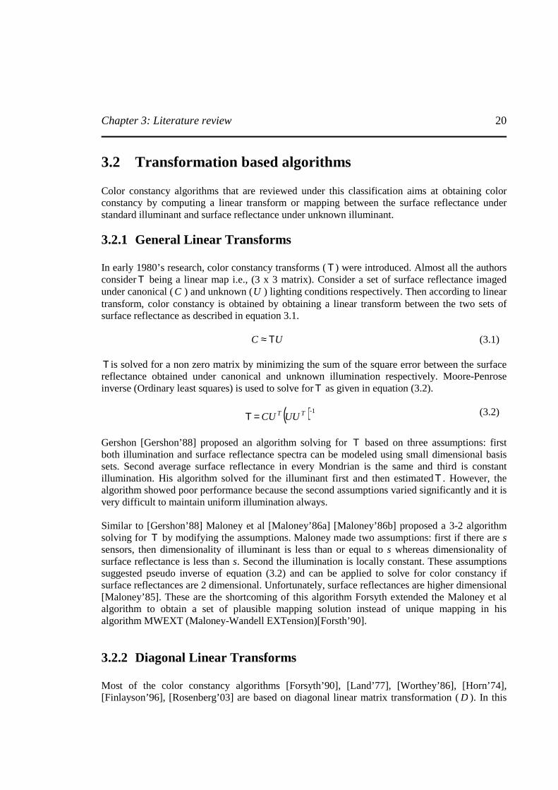
3.2.1 General Linear Transforms In early 1980’s research, color constancy transforms (Τ ) were introduced. Almost all the authors considerΤ being a linear map i.e., (3 x 3 matrix). Consider a set of surface reflectance imaged under canonical (C ) and unknown (U ) lighting conditions respectively. Then according to linear transform, color constancy is obtained by obtaining a linear transform between the two sets of surface reflectance as described in equation 3.1.
UC Τ≈ (3.1) Τ is solved for a non zero matrix by minimizing the sum of the square error between the surface reflectance obtained under canonical and unknown illumination respectively. Moore-Penrose inverse (Ordinary least squares) is used to solve forΤ as given in equation (3.2).
( ) -1TT UUCU=Τ (3.2)
Gershon [Gershon’88] proposed an algorithm solving for Τ based on three assumptions: first both illumination and surface reflectance spectra can be modeled using small dimensional basis sets. Second average surface reflectance in every Mondrian is the same and third is constant illumination. His algorithm solved for the illuminant first and then estimatedΤ . However, the algorithm showed poor performance because the second assumptions varied significantly and it is very difficult to maintain uniform illumination always. Similar to [Gershon’88] Maloney et al [Maloney’86a] [Maloney’86b] proposed a 3-2 algorithm solving for Τ by modifying the assumptions. Maloney made two assumptions: first if there are s sensors, then dimensionality of illuminant is less than or equal to s whereas dimensionality of surface reflectance is less than s. Second the illumination is locally constant. These assumptions suggested pseudo inverse of equation (3.2) and can be applied to solve for color constancy if surface reflectances are 2 dimensional. Unfortunately, surface reflectances are higher dimensional [Maloney’85]. These are the shortcoming of this algorithm Forsyth extended the Maloney et al algorithm to obtain a set of plausible mapping solution instead of unique mapping in his algorithm MWEXT (Maloney-Wandell EXTension)[Forsth’90].
3.2.2 Diagonal Linear Transforms Most of the color constancy algorithms [Forsyth’90], [Land’77], [Worthey’86], [Horn’74], [Finlayson’96], [Rosenberg’03] are based on diagonal linear matrix transformation (D ). In this
Chapter 3: Literature review
21
case, color constancy is obtained, by scaling each channel independently. Equation (3.1) is replaced by equation (3.3) in this case.
DUC ≈ (3.3) Solving for D using Moore-Penrose inverse (OLS), we get
( ) 3,2,1 -1
andiUUUCD Tii
Tiiii == (3.4)
West et al [West’82] showed that von Kries hypothesized that chromatic adaptation is a central mechanism for color constancy. It is based on the diagonal matrix transformation. The elements of the diagonal matrix in accordance to von Kries hypothesis is given by equation (3.5),
λλλ
λλλλ
ω
ω
dCI
dCIyxS
dk
k
k )( )(
)( )(),,(
∫
∫=
(3.5)
Finlayson [Finalyson’94] proposed a sensor sharpening method to improve the performance of the color constancy algorithms using diagonal matrix transformation to obtain color constancy. The efficiency of diagonal matrix also known as diagonal illumination model is an approximation function of sensors. The idea of sensor sharpening is to map the data by a linear transform into a new space where diagonal models are more reliable. Color constancy algorithms relying on diagonal transformation are more effective. The final result is then mapped back to original RGB space by taking the inverse transformation. Three types of sensor sharpening is proposed [Finlayson’94a] namely, sensor based sharpening, database sharpening and perfect sharpening. Besides these methods, there are other sensor sharpening methods proposed [Barnard’01]. The performance of the algorithms improved in terms of low rms error after performing sensor sharpening.
3.2.3 Gray World algorithm The gray world algorithm proposed by [Buchsbaum’80] is based on the gray world assumption. According to gray world assumptions the illuminant in each channel of the images averages to gray over the entire image. Any deviation from the gray value is due to the chromaticity shift of the illuminant. It is one of the important assumptions when trying to estimate the spectral distribution of the illuminant. A simple method of gray world assumption can be used find the average values of the image's R, G, and B color components and use their average to determine an overall gray value for the image. Each color component is then scaled independently according to the amount of it's deviation from this gray value. The scaling factors are obtained by simply dividing the gray value by the appropriate average of each color component. Thus if an image under normal white lighting satisfies the gray world assumption, putting it under a color filtered lighting would disrupt this behavior. By forcing the gray world assumption on the image again, it is in essence, removing the colored lighting to reacquire the true colors of the original. The expression in equation (3.6) is used to obtain gray world correction.
Chapter 3: Literature review
22
2
1)(
),.(1
)(
)(),.(1
),(I1
,
,,
∗=
=
=
∑
∑∑
k
N
yxkk
N
yxkk
N
yxk
I
yxSN
I
IyxSN
yxN
λ
λλ
λλ
(3.6)
where subscript k , represent the three color channel (R, G, and B) in color images and N is total number of pixels in image. From the equation (3.6) the illuminant RGB is twice the average of RGB image. However, if large database of real images are available, them the illuminant RGB is the ration of average image RGB to RGB of average of the reflectance database. This is referred as Database Gray World (DBGW) algorithm. GW algorithm is robust to illuminant color variation, but works for sequence with constant image average geometrical reflectance. In consequence, GW algorithm fails when new object appears in the images or when the illuminant geometry changes drastically.
3.2.4 Scale by max algorithm The scale by max algorithm estimates the illuminant by the maximum response in each channel. This algorithm is limited form of retinex algorithm [Horn’74]. Based on the maximum response in each channel, scaling factors are computed and each channel is scaled independently. The advantage of this method is, provided sufficient specularities and sufficient dynamic range of the vision system, the method provides an excellent estimate of the illuminant chromaticity. But this method is high sensitive to the dynamic range of the vision system. Scale by max algorithm is a subset of Bayesian algorithm [Brainard’97]. In Bayesian theory if the surface reflectance is assumed to be independent and uniform in the range of 0 and 1, then the maximum likelihood can be given by the equation (3.7).
),(I max ),,(I max ),,(I max,,,
yxIyxIyxIyx
bbyx
ggyx
rr === (3.7)
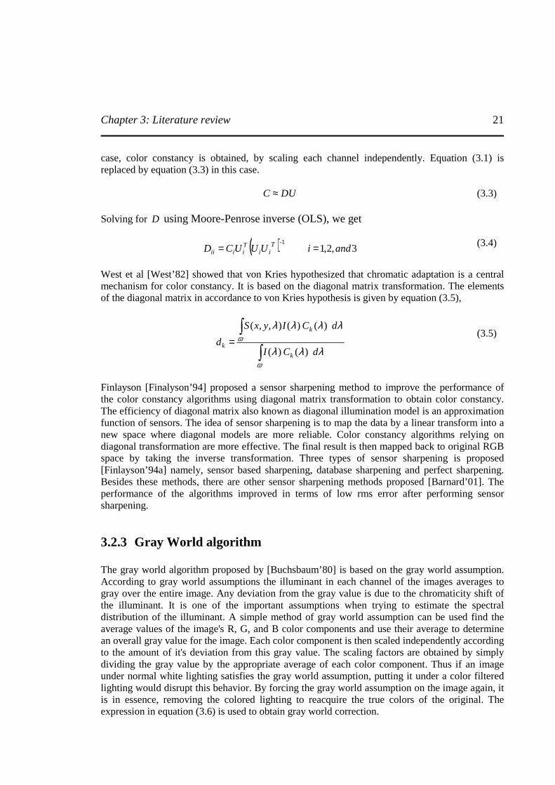
3.3 Retinex algorithm The Retinex theory introduced in late 1970’s by E. Land [Land’77] is based on the study of Retinex theory of image formation in human eyes. He studied the psychological aspects of lightness and color perception of human vision and proposed a theory to obtain an analogous performance in machine vision system. Retinex is not only used as a model for human vision color constancy, rather is also used as a platform for digital image enhancement, color constancy, and lightness/color rendition. Land’s Retinex theory is based on the design of surround function. Initial, 1/r2 surround function proposed by Land [Land’77] was replaced by a Gaussian surround

Chapter 3: Literature review
23
function by Hurlbert [Hurlbert’89] by choosing three different sigma values to achieve the good dynamic range compression and color rendition. The sigma values are also known as surround constants ( ic ). The Gaussian surround function is given by the expression in equation (3.8)
3 and 2 ,1 ,
),(22
2
=+=
= −
iyxr
eyxF icr
(3.8)
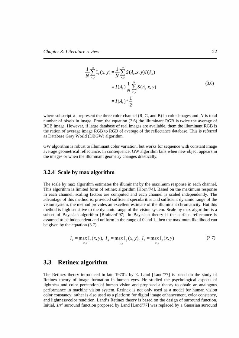
The reasons for selecting three different sigma or surround constant are, (a) For small sigma value (c1=80), the surround function acts as a high pass filter, capturing fine details of the image but at a loss of tonal information. (b) For high value of sigma (c3=250), the surround function captures the tonal information at the cost of fine details. (c) For medium value of sigma (c2=120), the surround function captures both dynamic range and tonal information. From that point onwards, number of different implementation of Retinex theory has been presented like [Funt’04], [Funt’97b], [Barnard’98], [McCann’83], [Kimmel’03], [Rahman’97], [Rizzi’04], [Cooper’04], [Rising III’04] and effort is been made to optimize the performance of the Retinex algorithm by tuning the parameters using the approaches mentioned in [Ciurea’04], [Funt’01]. The Multiscale retinex (MSR) implementation of [Rahman’97] intertwined number of image processing operations and as a result, the colors are changed in images dependent and unpredicted ways. K. Barnard and B. Funt in there work [Barnard'98] and [Funt’97b] respectively presented a way to make MSR operation more clear and to ensure color fidelity. They disentangled these tasks and the color balance is provided using a neural network color constancy method described in [Funt’96]. In the next step, MSR is applied to the image luminance as described in [Barnard’98]. The figure 3.2 shows the distributions of Gaussian surround function for different values of sigma.
Chapter 3: Literature review
24
(a)
(b)
Figure 3.2 Gaussian distribution of the surround functions for different sigma values. (a) c1 = 80, (b) c2 =
120, and (c) c3 = 250.
Chapter 3: Literature review
25
(c)
Figure 3.2 Continued.
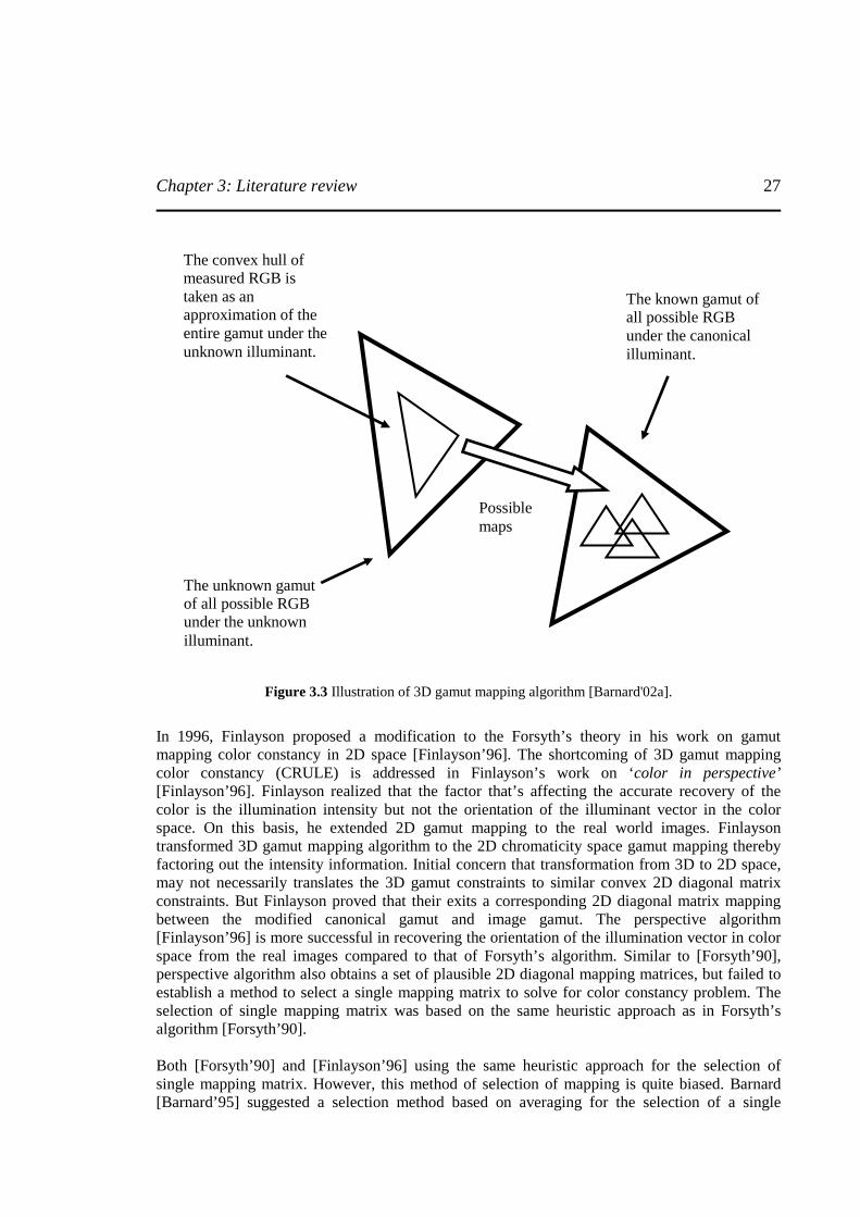
3.4 Gamut algorithms The concept of gamut approach is based on the works of Forsyth in early 1990’s. The constraint based algorithms [Forsyth’90], [Finlayson’96], [Finlayson’98], [Finlayson’99] achieve color constancy by imposing constraints on the scene and / or illuminant of the scene. Forsyth proposed an algorithm called ‘Gamut mapping’. The implementation trick of the gamut algorithms is based on the knowledge of the canonical illuminants from which the surface reflectance of the image can be computed. These algorithms impose pretty hard constraints on the range of occurrence of the illuminant. The constraint is due to the fact that surface can reflect no more light than is cast on them. For example, if one observes a scene / or patch that excites red photoreceptors of the sensors, then under no circumstances the illuminant can be blue. Therefore the range of illuminant used in computation of color constancy is very limited in these cases. The gamut mapping algorithms for color constancy works well under supervised conditions and with prior knowledge of canonical illuminant. This method is also known as 3D gamut mapping because color constancy is computed in 3D RGB space. The algorithm is a two step process. In the first step two possible gamuts are obtained namely, the canonical gamut and the image gamut (also known as unknown illuminant gamut). Canonical gamut ( )( )CG is obtained by taking all the set of possible (R, G, B) due to
Chapter 3: Literature review
26
surfaces under canonical illuminants, with the choice of the canonical illuminant being arbitrary. Similarly, image gamut ( )( )IG ′ is obtained from a set of all possible (R, G, B) due to surface reflectance under unknown illumination. Both the gamuts are convex and are represented by convex hull. In the second step, under diagonal assumptions [Forsyth’90], both the convex hulls can be mapped uniquely to each other. The objective is to obtain the diagonal mapping. The image gamut is mapped into a canonical gamut using a linear mapping. Forsyth developed a procedure called MWEXT [Forsyth’90]. MWEXT requires both the surface reflectance and illuminants to be selected from a finite dimensional space. It presented three challenges, (1) Conditions necessary to use linear mapping is too restrictive. (2) Linear maps required nine parameters which implied solving nine dimensional problems. Thus it is too computationally expensive. (3) Not all the linear maps correspond to plausible changes in illumination. Forsyth suggested an algorithm CRULE to solve for MWEXT problems. CRULE will work for any reflectance surface. CRULE corresponds to a form of coefficient rule which is obtained using the illuminant constraint. In CRULE, illuminant maps are restricted to three parameter diagonal matrix. Thus gamut mapping color constancy attempts to determine the set of diagonal matrices taking the image gamut into the canonical gamut. The 3x3 diagonal maps (D ) are given by expression in equation (3.9).
( ) ( )CpDIp , ,', ∈∈∀−−
(3.9)
Forsyth [Forsyth’90] adopted a heuristic approach to select single diagonal mapping from a set of plausible mappings. Mapping which maximized the volume of the mapped set, i.e. diagonal transform with maximum determinant was selected as a single diagonal matrix taking image gamut to the canonical gamut. Figure 3.3 illustrates the basic idea of gamut mapping color constancy. Gamut mapping color constancy is based on the assumptions that all the surfaces in the images are flat; there are no shadows, no mutual illumination and uniform single illuminant. It also assumes that all the surfaces are Lambertian and have diffuse surface reflection. Any violations of the assumptions confound the 3D gamut mapping algorithms. 3D gamut mapping method fails when presented with images with many illuminants and dynamic illumination variation across the image. However, most of these assumptions are not true in practice. Therefore 3D gamut mapping algorithm is very restricted. Thus the Forsyth’s stated that CRULE algorithm’s performance is strictly based on the linear illuminant change assumptions. Under varying illumination conditions, variation in shape and occurrence of specular highlights, these assumptions are violated, thereby CRULE fails.
Chapter 3: Literature review
27
Figure 3.3 Illustration of 3D gamut mapping algorithm [Barnard'02a].
In 1996, Finlayson proposed a modification to the Forsyth’s theory in his work on gamut mapping color constancy in 2D space [Finlayson’96]. The shortcoming of 3D gamut mapping color constancy (CRULE) is addressed in Finlayson’s work on ‘color in perspective’ [Finlayson’96]. Finlayson realized that the factor that’s affecting the accurate recovery of the color is the illumination intensity but not the orientation of the illuminant vector in the color space. On this basis, he extended 2D gamut mapping to the real world images. Finlayson transformed 3D gamut mapping algorithm to the 2D chromaticity space gamut mapping thereby factoring out the intensity information. Initial concern that transformation from 3D to 2D space, may not necessarily translates the 3D gamut constraints to similar convex 2D diagonal matrix constraints. But Finlayson proved that their exits a corresponding 2D diagonal matrix mapping between the modified canonical gamut and image gamut. The perspective algorithm [Finlayson’96] is more successful in recovering the orientation of the illumination vector in color space from the real images compared to that of Forsyth’s algorithm. Similar to [Forsyth’90], perspective algorithm also obtains a set of plausible 2D diagonal mapping matrices, but failed to establish a method to select a single mapping matrix to solve for color constancy problem. The selection of single mapping matrix was based on the same heuristic approach as in Forsyth’s algorithm [Forsyth’90]. Both [Forsyth’90] and [Finlayson’96] using the same heuristic approach for the selection of single mapping matrix. However, this method of selection of mapping is quite biased. Barnard [Barnard’95] suggested a selection method based on averaging for the selection of a single
Possible maps
The convex hull of measured RGB is taken as an approximation of the entire gamut under the unknown illuminant.
The unknown gamut of all possible RGB under the unknown illuminant.
The known gamut of all possible RGB under the canonical illuminant.

Chapter 3: Literature review
28
mapping from a set of feasible mapping in both chromaticity space and RGB space. This method is based on the assumption that all the illuminant and their corresponding mapping are equally probable. Under such assumption, mean or expected value is used for the selection of the single mapping. This approach improved the results compared to the heuristic approach adopted in [Forsyth’90], [Finlayson’96]. However in 2D perspective method unwanted distortion affected the mapping sets; therefore suggesting that 2D mean estimation for selection of single mapping is biased in chromaticity space. Therefore Finlayson [Finlayson’99] suggested mean estimation from the reconstructed 3D maps. In figure 3.4, the perspective maps are converted to three vectors. Thus a cone with vertex at origin passing through all the extreme points of mapping is obtained in the plane γ =1. Equal probability of occurrence of maps is assumed. Monte Carlo integration is performed to obtain the 3D mean [Finlayson’99], [Barnard’02a]. Figure 3.4 also shows the disparity between the mean estimated using 2D perspective and 3D gamut. In 2000, Finlayson proposed two new methods for mapping selection [Finlayson’00]. Angular error between selected set of feasible mappings was used to select single mapping. The mapping for which the angular error is least is selected as the best diagonal map. He also replaced mean approach with the median approach.
Figure 3.4 The convex polygon denotes the gamut of feasible mapping calculated by 2D perspective. The cone bounds the corresponding 3D set. The mean of the perspective gamut of mapping (open circle) is
quite different from the mean calculated in 3D (filled circle) [Finlayson’99].
β
γ
α
γ = 1
3d mean
2d mean
Chapter 3: Literature review
29
3.5 Statistical color constancy algorithms The color constancy algorithms discussed under this classification follow the basic statistical assumptions, of normal distribution of the data, i.e., the probability distribution is Gaussian and maximum likelihood is used as parameter estimator. However, there are some algorithms, that experiment with different probability distribution [Rosenberg’03] and parameter estimators [Rosenberg’01], [Freeman’95], [Brainard’97].
3.5.1 Bayesian algorithm Bayesian theory on color constancy [Freeman’95] provides an insight on how to use all the information about the illuminant contained in the sensor response, including the information used by the gray world and physical reliability algorithms. Three probabilities play an important role in the Bayesian theory, namely the prior, likelihood and the posterior probability. The prior probability is the information about the known parameters before observing the data. For explanation, if parameter is described by vectorx , then prior is the probability density given by )(xp . The Likelihood )/( xyp computes the relationship between the data y and the parametersx . Once the prior and likelihood is known, the posterior is computed using Baye’s rule given in equation (3.10),
)(
)()/()/(
yp
xpxypyxp =
(3.10)
Most of the color constancy algorithms [Land’77], [Funt’96], [Finlayson’95] assumes a prior knowledge on the illumination distribution. Prior knowledge on the occurrence of the illumination can be assumed to be uniform, i.e., probability of occurrence of all the illuminants is equal. This approach is fair if the range of occurrence of the illuminant is not known. Alternatively if the range occurrence of the illuminants is known, then prior information on the illuminant can be estimated from a specified set of images within that range. Bayesian framework for color constancy is a three step process. First, the relation between the reflectance, illuminants and sensor responses is established. Second the prior information of illuminants and surfaces of existence in the world is computed. Finally, using the Baye’s rule, posterior distribution of the illuminant and surfaces in the scene is obtained. There are two most commonly used methods for obtaining the best estimate from the posterior distribution. These are maximum a posteriori (MAP) and minimum mean squared error (MMSE). Former is similar to the maximum likelihood technique used in many statistical theories. D. H. Brainard and W. T. Freeman in their work on Bayesian based color constancy [Freeman’95], [Brainard’97] proposed a bilinear modeling technique. This means that for a fixed spectral distribution, relation between reflectance and sensor responses is linear and for fixed sensor response, relation between spectral distribution and reflectance is linear. They showed that the reflectance and spectral information can be obtained by solving for the linear models of weights of surface reflectance and illumination spectrum. The bilinearity implied that estimation of weights is ill-posed because different combination of weights may provide same sensor
Chapter 3: Literature review
30
measurement. Therefore in [Freeman’95], [Brainard’97] a statistical distribution of the illuminant is obtained using conditional probability density function to cope with the ill-posedness. Normal distribution of the image data for a given illumination is assumed. The likelihood is computed using the expression in equation (3.11). In [Freeman’95], [Brainard’97] prior estimation is obtained by using principal component analysis (PCA) to obtain the best estimation of the spectral distribution.
)( ,2
1)/(
2
2
2
)(
2xfyexyp
xfy
==−−
σ
πσ,
(3.11)
Both [Freeman’95], and [Brainard’97], proposed a new method to obtain the best estimate from the posterior distribution, namely maximum local mass (MLM) that integrates over local probability density. MAP estimation method neglected variations in the shape of ridge of the posterior distribution which can be a significant source of information. The MMSE method is sensitive to the structure of the posterior therefore it may lead to a very unlikely estimation. However MLM approach required intense optimization routine and is computationally expensive. In 2002, Skaff et al [Skaff’02], proposed an extension to the works of W. H. Freeman and D. H. Brainard. They showed that [Freeman’95] [Brainard’97] approach is extendable to multiple non uniform sensors. They developed multi-sensor Bayesian technique for color constancy by sequentially acquiring measurements from independent sensors. They presented two cases: (a) two sets of sensors with independent sensor sensitivity, and (b) a continuous variation in the spectral sensitivities across the sensor arrays. Bayesian chaining approach is used in both the cases. In Bayesian chaining approach, posterior is continuously updated by using the posterior computed in the previous stage as a prior for the next stage. MLM estimation technique is used to obtain the best estimation of the posterior distribution. In 2001, Tsin et al [Tsin’01], improved the Bayesian work presented in [Freeman’95], [Brainard’97] by adapting the technique for outdoor object recognition. They proposed a simple bilinear diagonal color model and an iterative linear update method based on MAP estimation technique. A finite dimensional linear models is used for both reflectance [Maloney’86b] and illuminant spectrum [Slater’98] to obtain a bilinear color model. Statistical distribution of the illuminant is learned by observing F frames of P pixel patch under uniform illumination to obtain a color measurement matrix. Singular value decomposition (SVD) of color measurement matrix is performed to obtain the estimate of the reflectance and spectral matrix. Baye’s rule is used to obtain the posterior distribution. In this method, prior is computed using the illumination information from the patch under investigation. In 2003, Rosenberg et al [Rosenberg’03] presented Bayesian framework for color constancy using non Gaussian models. In [Rosenberg’03], independent and Gaussian distribution of the reflectance [Freeman’95] [Brainard’97] is replaced by an exchangeable reflectance distribution. The reflectance is defined by a Dirichlet-multinomial model. Based on multinomial distribution, the likelihood is computed using the expression in equation (3.12)

Chapter 3: Literature review
31
)()/( 11 YLXpLlYpn −− ==
(3.12)
The quantity YL 1− is computed using equation (3.12) and can also be referred as Likelihood corrected image. Here L is a diagonal illumination matrix. The posterior is computed by assuming a uniform prior. Rosenberg et al [Rosenberg’01] also proposed KL Divergence approach for parameter estimation instead of maximum likelihood approach. The parameter estimation is performed in logarithmic chromaticity space instead of RGB color space. Performance measure of both maximum likelihood and KL Divergence method present two analyses. Maximum likelihood estimation is more sensitive to large peaks in the observed distribution, whereas KL divergence is less sensitive to the large peaks. Secondly, in maximum likelihood the best estimate of obtained when as many of the observed colors as possible are aligned with high likelihood in canonical distribution. In case of KL Divergence best estimate is observed when observed distribution is most similar to the canonical distribution. Both [Rosenberg’03], and [Rosenberg’01], obtained the color distribution using the approach described in [Funt’99] on real image database. A simple color constancy algorithm is used as a base algorithm to establish a proxy ground truth.
3.5.2 Color by correlation algorithm Finlayson introduced a new method to estimate the illuminant chromaticity and achieve color constancy, while addressing the assumptions of other color constancy algorithms such as presence of white patch in every image [Land’77], and the average reflectance of all the surfaces in a scene is achromatic [Buchsbaum’80], [Gershon’88]. This new illuminant estimation algorithm is based on a correlation framework in two dimensional chromaticity space [Finlayson’01], [Finlayson’97]. In this framework, the illuminant estimation is posed on a correlation of the color in the image and the prior knowledge about the colors that can appear under that light. Color by correlation algorithm estimates the illuminant chromaticity in the chromaticity space and assumes a two dimensional world in which all the objects are flat, matte and Lambertian surfaces, uniformly illuminated. Besides these assumptions, the color by correlation algorithm makes two more assumptions. First, that a given device will produce responses only within a finite region of the data, i.e., the chromaticity coordinates will range from 0 to 1. Second, the chromaticity space is sampled into uniform bins of NN ∗ regions. In this approach, correlation matrix to correlate all possible colors with each of the set of possible scene illuminant is created by taking the probability distribution of each illuminant. This probability is encoded as columns of correlation matrix. The procedure is shown in figure 3.5. The chromaticity present in the uncorrected images is estimated and presented as a binary vector. The correlation between the binary vector and the correlation matrix is established using a dot product rule. The illuminant that is highly correlated is given by the maximum dot product value. The process is illustrated in figure 3.6. Logarithmic likelihood is computed and then using a Bayes equation posterior distribution is computed.

Chapter 3: Literature review
32
Figure 3.5 Three steps to build correlation matrix [Finalson’01]. (a) Distribution of reference images
chromaticities. (b) Probability distribution for each light. (c) Encoding the distribution in the column of the matrix.
Figure 3.6 Three steps to solve for color constancy [Finalson’01]. (a) Histogram of the chromaticity in the image. (b) Correlation measure between image vector ( v ) and the correlation matrix ( M ).

Chapter 3: Literature review
33
Inspired by the work of gamut mapping algorithm in both 2D and 3D space, color by correlation [Finlayson’01] is extended to 3D space by K. Barnard et al in his work [Barnard’00a]. The reason for 2D to 3D space extension is based on two observations. First pixel brightness makes significant contribution to the color constancy. Second, the use of its statistical knowledge about the world is also useful for color constancy. Based on these inferences, color by correlation for three dimensional spaces is proposed. However, the success of the algorithm on synthetic data set is not seen on a data set of 321 calibrated real images. The other color constancy algorithm that uses correlation framework is proposed by Sapiro [Sapiro’99].
3.6 Learning theory based algorithms First learning theory based work on color constancy performed in late 1990’s is neural networks based color constancy [Cardei’00]. Other works on neural network based color constancy involves [Funt’99a], [Funt’97a], [Cardei’99b], [Cardei’97], [Cardei’02] and [Ebner’04]. Neural network based color constancy is performed in 2D chromaticity space. The network is trained using gradient based algorithms that minimize the networks output error by re-adjustments of the neuron weights. The network architecture proposed by V. Cardei [Cardei’00], [Cardei’02], [Funt’99] consisting of 3600 input nodes, 400 neurons in first hidden layer, 40 neurons in second hidden layer and two output neurons is trained for both the experimentation on synthetic and real images. The training data’s are converted into chromaticity space. The chromaticity space is uniformly sampled to obtain 2D chromaticity histogram. The sampling rate defines the size of the input nodes in the network architecture. The 2D chromaticity space is binarized in 0’s and 1’s indicating the presence of chromaticity bins (1’s) and absence of chromaticity bins (0’s) in the training images. To reduce the dimensionality of the network only the active bins were provided to the network during training. The target chromaticity values of the training data is obtained estimated using simple color constancy algorithm. Gray world algorithm is used to estimate the target chromaticity values. Training time of the network was reduced by using adaptive learning rate [Cardei’02] [Cardei’00]. The neural net based color constancy experimentation is performed on both synthetic and real images [Cardei’00], [Cardei’02]. Both the experimentation has its own pros and cons. To synthesize scene, requires knowledge about the camera characteristics and spectral distribution of the illuminant. Moreover the affect of noise and specularities in real images are not taken into consideration which limits the performance of the trained network on the real images. In the case of real images, very large numbers of real images are required to train the network. Neural network training using real images requires significantly large number of real images. Due to practical limitation to collect such large number of images, Cardei and Funt [Funt’99] applied a statistical approach [Chernick’99] known as “Bootstrapping” to generate large number of training images from small number of real images. This approach generates a large number of training images from a limited sample of images by sub-sampling the given set of images. Here sampling rate defines the number of training images generated from an each image in the sample. The evaluation showed that neural network trained based on the GW estimate performed better than GW algorithm. According to [Funt’99] the performance of network trained on GW estimate has high mean error and low standard deviation when compared to the network trained on exact illuminant data.
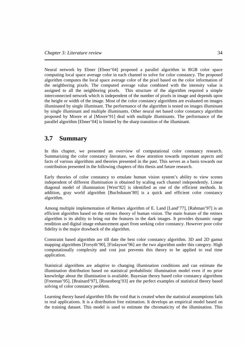
Chapter 3: Literature review
34
Neural network by Ebner [Ebner’04] proposed a parallel algorithm in RGB color space computing local space average color in each channel to solve for color constancy. The proposed algorithm computes the local space average color of the pixel based on the color information of the neighboring pixels. The computed average value combined with the intensity value is assigned to all the neighboring pixels. This structure of the algorithm required a simple interconnected network which is independent of the number of pixels in image and depends upon the height or width of the image. Most of the color constancy algorithms are evaluated on images illuminated by single illuminant. The performance of the algorithm is tested on images illuminant by single illuminant and multiple illuminants. Other neural net based color constancy algorithm proposed by Moore et al [Moore’91] deal with multiple illuminants. The performance of the parallel algorithm [Ebner’04] is limited by the sharp transition of the illuminant.
3.7 Summary In this chapter, we presented an overview of computational color constancy research. Summarizing the color constancy literature, we draw attention towards important aspects and facts of various algorithms and theories presented in the past. This serves as a basis towards our contribution presented in the following chapters of this thesis and future research. Early theories of color constancy to emulate human vision system’s ability to view scenes independent of different illumination is obtained by scaling each channel independently. Linear diagonal model of illumination [West’82] is identified as one of the efficient methods. In addition, gray world algorithm [Buchsbaum’80] is a quick and efficient color constancy algorithm. Among multiple implementation of Retinex algorithm of E. Land [Land’77], [Rahman’97] is an efficient algorithm based on the retinex theory of human vision. The main feature of the retinex algorithm is its ability to bring out the features in the dark images. It provides dynamic range rendition and digital image enhancement apart from seeking color constancy. However poor color fidelity is the major drawback of the algorithm. Constraint based algorithm are till date the best color constancy algorithm. 3D and 2D gamut mapping algorithms [Forsyth’90], [Finlayson’96] are the two algorithm under this category. High computationally complexity and cost just prevents this theory to be applied to real time application. Statistical algorithms are adaptive to changing illumination conditions and can estimate the illumination distribution based on statistical probabilistic illumination model even if no prior knowledge about the illumination is available. Bayesian theory based color constancy algorithms [Freeman’95], [Brainard’97], [Rosenberg’03] are the perfect examples of statistical theory based solving of color constancy problem. Learning theory based algorithm fills the void that is created when the statistical assumptions fails in real applications. It is a distribution free estimation. It develops an empirical model based on the training dataset. This model is used to estimate the chromaticity of the illumination. This

Chapter 3: Literature review
35
approach is adaptive. Neural network is the only learning theory algorithm developed till date. Its instability and large training time is the major limitation of the method. We present the comparison of state of art of color constancy research in table 3.1. This completes the review of literature and in the following chapters we present extension of the literature in form of our contribution.

Chapter 3: Literature review
36
Table 3.1 Comparison of color constancy classification based on advantages and disadvantages.
Color constancy literature
classification Advantages Disadvantages
Simple color constancy algorithms
Computationally less expensive. Analytical solution is possible.
Less reliable and not adaptive. Highly dependent on assumptions.
Retinex algorithms Improves the image visual appearance. Good performance on dark images.
Poor color fidelity. Large number of free parameters to be optimized.
Constraint based algorithms Best color reproduction (color constancy).
Computationally very expensive. Dependency on the sensor sensitivity information. Assumes uniform illumination over entire scene. Dependency on the knowledge of the range of illuminant.
Statistical algorithms Adaptive to changing illumination condition. The illumination distribution is obtained from the knowledge of statistical probabilistic distribution No prior knowledge of the illumination is required.
In real time statistical assumptions are violated. Computationally expensive.
Learning theory algorithm Adaptive to changing illumination condition. Can perform color constancy from very approximate knowledge of illumination chromaticity.
Unstable. High training time. Computationally very expensive. Difficult to regularize the estimation of illuminant chromaticity.
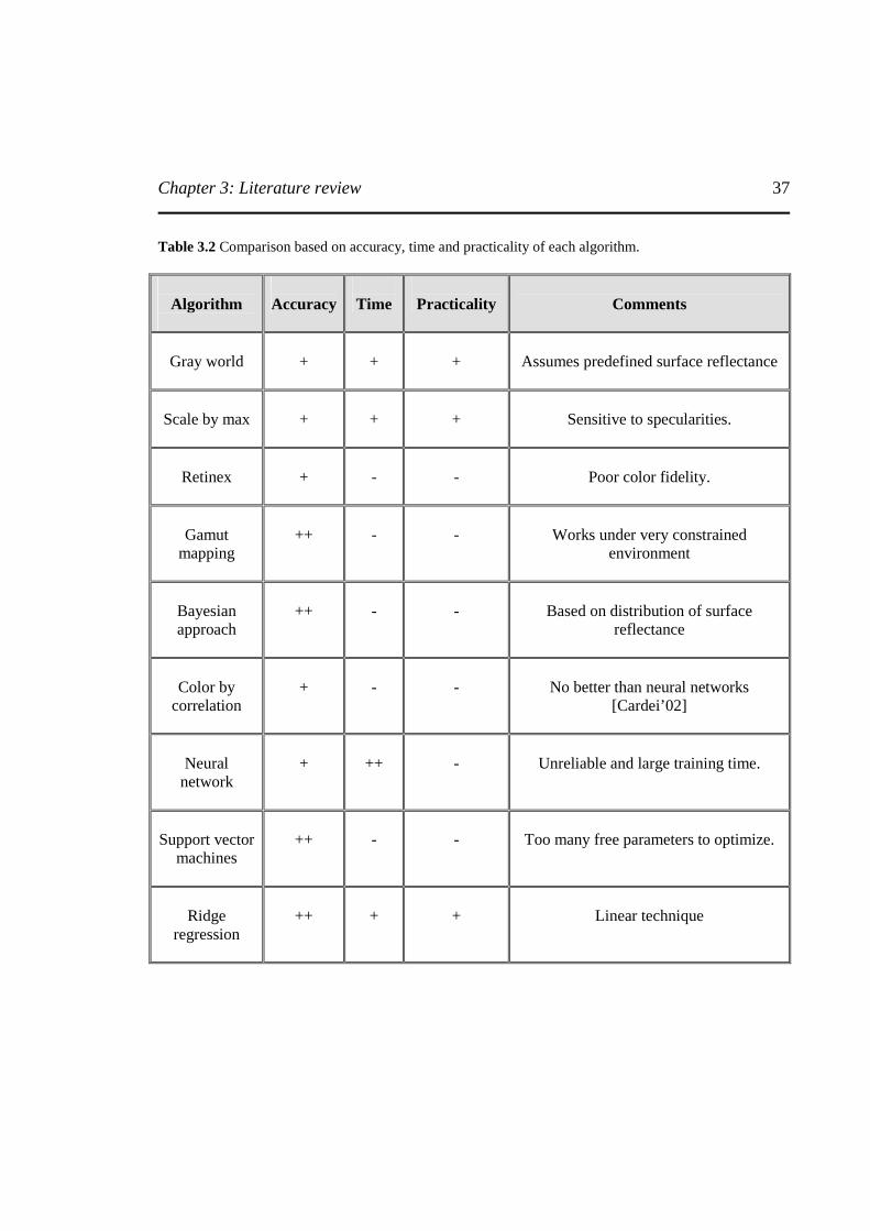
Chapter 3: Literature review
37
Table 3.2 Comparison based on accuracy, time and practicality of each algorithm.
Algorithm
Accuracy
Time
Practicality
Comments
Gray world
+
+
+
Assumes predefined surface reflectance
Scale by max
+
+
+
Sensitive to specularities.
Retinex
+
-
-
Poor color fidelity.
Gamut
mapping
++
-
-
Works under very constrained
environment
Bayesian approach
++
-
-
Based on distribution of surface
reflectance
Color by
correlation
+
-
-
No better than neural networks
[Cardei’02]
Neural network
+
++
-
Unreliable and large training time.
Support vector
machines
++
-
-
Too many free parameters to optimize.
Ridge
regression
++
+
+
Linear technique
Chapter 4: Neural network based color constancy
38
Chapter 4
4 NEURAL NETWORK BASED COLOR CONSTANCY This chapter presents discussion on the neural networks architecture, activation functions, backpropagation algorithm, and application of neural network in solving for color constancy. Neural network is a learning theory based modeling tool aimed to approximate specific human brain activity. The simplest form of neural network introduced in 1962 by Rosenblatt [Rosenblatt’62], a single layer networks with threshold activation function, is known as ‘perceptron’. A single perceptron is a processing element with an ability to learn iteratively under supervised conditions. The same is extended to solve for regression by Widrow et al [Widrow’90]. He called it as ‘adaline’ derived from ADAptive LINear Element. Due to the limitation of the single layer perceptron, it is extended to multilayer perceptron. Multilayer perceptron is a feed forward network trained using back propagation algorithm. The learning ability of the network paved way for the researchers solving for color constancy to evaluate its performance in emulating human color constancy. The subsection 4.1 discusses single layer perceptron and multi-layer perceptron. Subsection 4.2 talks about the activation functions. Back propagation algorithm is discussed in subsection 4.3. Subsection 4.4 presents a detailed theory on the usage of neural network to learn color and correct for color deviation. Finally limitations and advantages of network are presented in subsection 4.5.
4.1 Single layer perceptron and Multi-layer perceptron The perceptron is a single processing element introduced by Rosenblatt [Rosenblatt’62] in 1962 to solve for applications like pattern recognition by autonomous adjustment of the weights using data pairs. The weight adjustment feature is adaptive and gradually reduces the error towards zero. Thus perceptron is able to learn iteratively under supervised learning paradigm. However the initialization of the weights is a random process, but over the process of learning for a selected input data vector ‘x’, the perceptron readjusts the weights based on the desired output vector. The perceptron can classify two classes of pattern successfully if they were linearly separable. The output of the perceptron is mathematically given by equation (4.1),
= ∑
=i
n
ii xwu
1
(4.1)
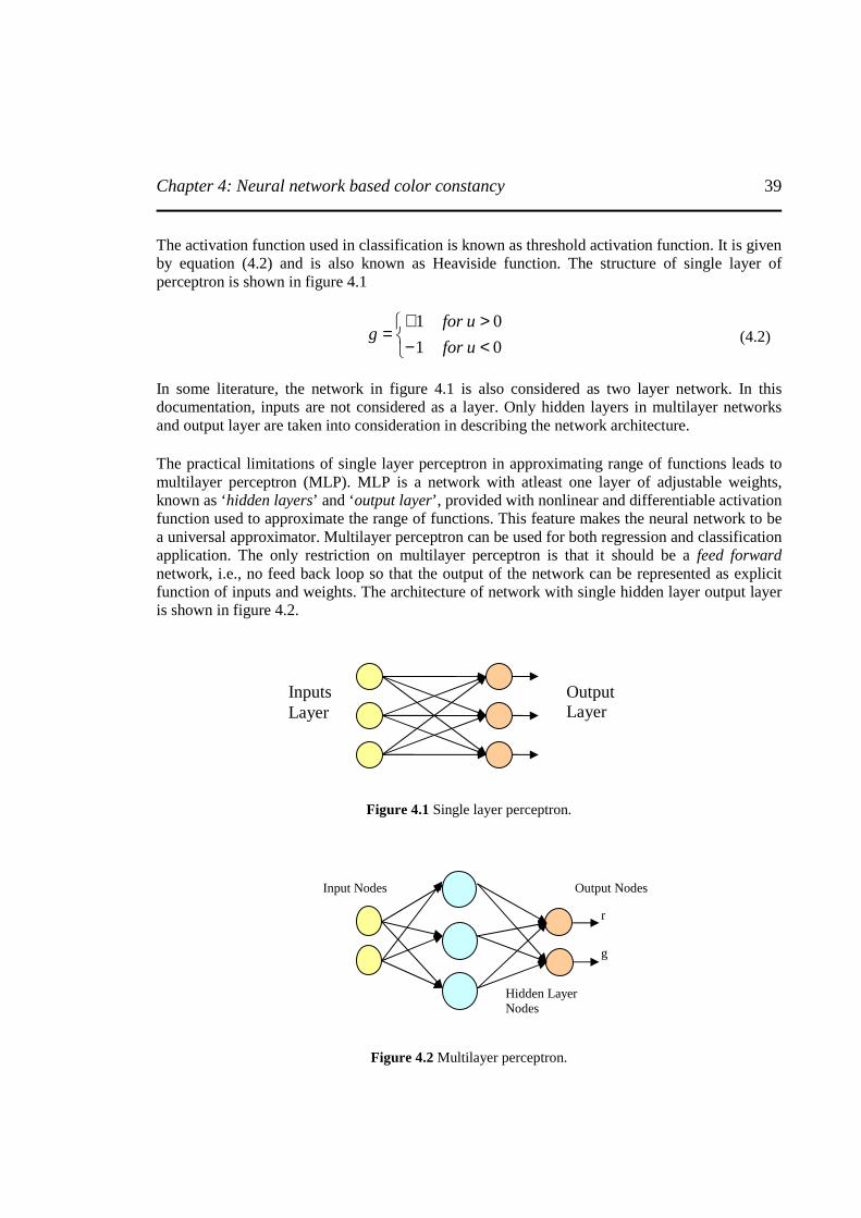
Chapter 4: Neural network based color constancy
39
The activation function used in classification is known as threshold activation function. It is given by equation (4.2) and is also known as Heaviside function. The structure of single layer of perceptron is shown in figure 4.1
<−>+
=0 1
0 1
ufor
uforg
(4.2)
In some literature, the network in figure 4.1 is also considered as two layer network. In this documentation, inputs are not considered as a layer. Only hidden layers in multilayer networks and output layer are taken into consideration in describing the network architecture. The practical limitations of single layer perceptron in approximating range of functions leads to multilayer perceptron (MLP). MLP is a network with atleast one layer of adjustable weights, known as ‘hidden layers’ and ‘output layer’, provided with nonlinear and differentiable activation function used to approximate the range of functions. This feature makes the neural network to be a universal approximator. Multilayer perceptron can be used for both regression and classification application. The only restriction on multilayer perceptron is that it should be a feed forward network, i.e., no feed back loop so that the output of the network can be represented as explicit function of inputs and weights. The architecture of network with single hidden layer output layer is shown in figure 4.2.
Figure 4.1 Single layer perceptron.
Figure 4.2 Multilayer perceptron.
Inputs Layer
Output Layer
Input Nodes
Output Nodes
Hidden Layer Nodes
r
g
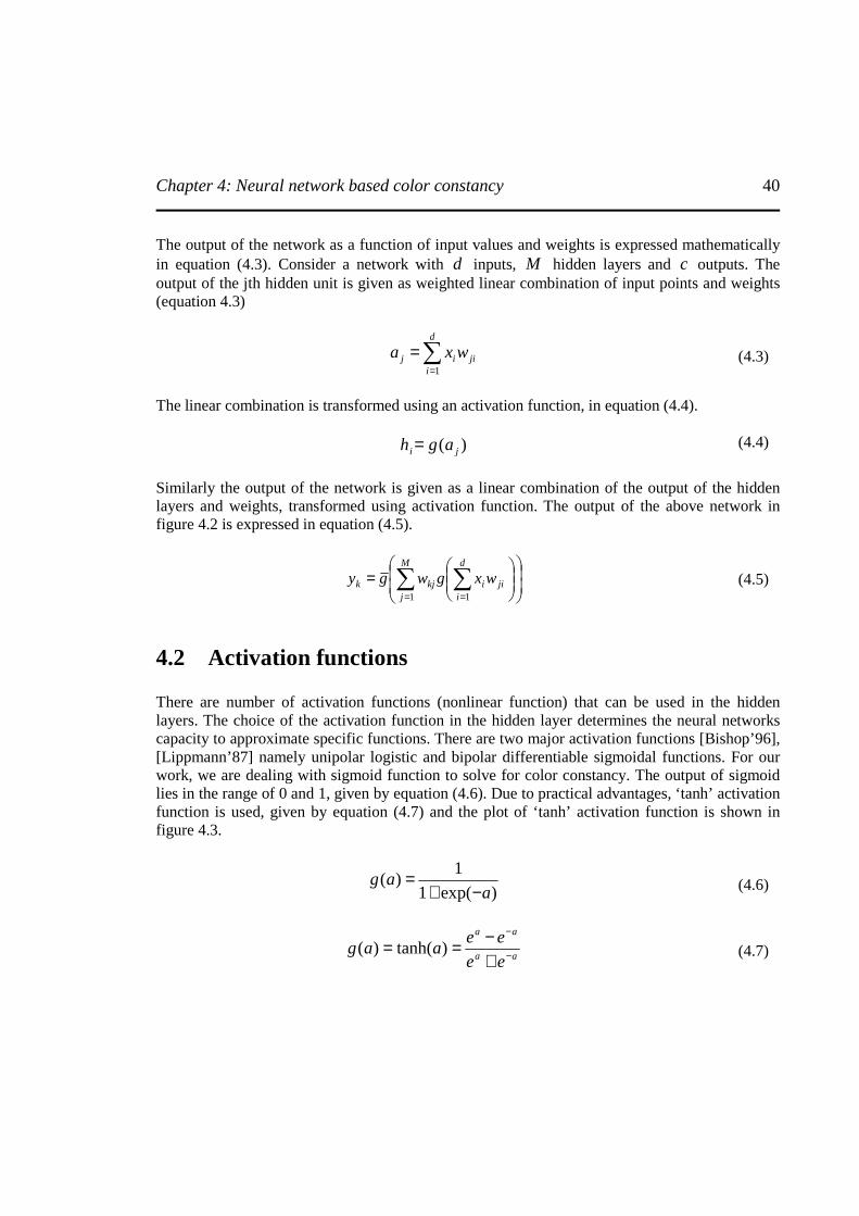
Chapter 4: Neural network based color constancy
40
The output of the network as a function of input values and weights is expressed mathematically in equation (4.3). Consider a network with d inputs, M hidden layers and c outputs. The output of the jth hidden unit is given as weighted linear combination of input points and weights (equation 4.3)
∑=
=d
ijiij wxa
1
(4.3)
The linear combination is transformed using an activation function, in equation (4.4).
)( ji agh = (4.4)
Similarly the output of the network is given as a linear combination of the output of the hidden layers and weights, transformed using activation function. The output of the above network in figure 4.2 is expressed in equation (4.5).
= ∑∑
==
d
ijii
M
jkjk wxgwgy
11
(4.5)
4.2 Activation functions There are number of activation functions (nonlinear function) that can be used in the hidden layers. The choice of the activation function in the hidden layer determines the neural networks capacity to approximate specific functions. There are two major activation functions [Bishop’96], [Lippmann’87] namely unipolar logistic and bipolar differentiable sigmoidal functions. For our work, we are dealing with sigmoid function to solve for color constancy. The output of sigmoid lies in the range of 0 and 1, given by equation (4.6). Due to practical advantages, ‘tanh’ activation function is used, given by equation (4.7) and the plot of ‘tanh’ activation function is shown in figure 4.3.
)exp(1
1)(
aag
−+=
(4.6)
aa
aa
ee
eeaag −
−
+−== )tanh()(
(4.7)
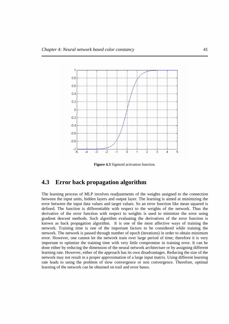
Chapter 4: Neural network based color constancy
41
Figure 4.3 Sigmoid activation function.
4.3 Error back propagation algorithm The learning process of MLP involves readjustments of the weights assigned to the connection between the input units, hidden layers and output layer. The learning is aimed at minimizing the error between the input data values and target values. So an error function like mean squared is defined. The function is differentiable with respect to the weights of the network. Thus the derivative of the error function with respect to weights is used to minimize the error using gradient descent methods. Such algorithm evaluating the derivatives of the error function is known as back propagation algorithm. It is one of the most affective ways of training the network. Training time is one of the important factors to be considered while training the network. The network is passed through number of epoch (iterations) in order to obtain minimum error. However, one cannot let the network train over large period of time; therefore it is very important to optimize the training time with very little compromise in training error. It can be done either by reducing the dimension of the neural network architecture or by assigning different learning rate. However, either of the approach has its own disadvantages. Reducing the size of the network may not result in a proper approximation of a large input matrix. Using different learning rate leads to using the problem of slow convergence or non convergence. Therefore, optimal learning of the network can be obtained on trail and error bases.
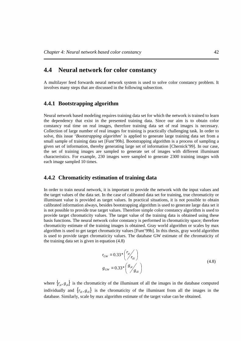
Chapter 4: Neural network based color constancy
42
4.4 Neural network for color constancy A multilayer feed forwards neural network system is used to solve color constancy problem. It involves many steps that are discussed in the following subsection.
4.4.1 Bootstrapping algorithm Neural network based modeling requires training data set for which the network is trained to learn the dependency that exist in the presented training data. Since our aim is to obtain color constancy real time on real images, therefore training data set of real images is necessary. Collection of large number of real images for training is practically challenging task. In order to solve, this issue ‘Bootstrapping algorithm’ is applied to generate large training data set from a small sample of training data set [Funt’99b]. Bootstrapping algorithm is a process of sampling a given set of information, thereby generating large set of information [Chernick’99]. In our case, the set of training images are sampled to generate set of images with different illuminant characteristics. For example, 230 images were sampled to generate 2300 training images with each image sampled 10 times.
4.4.2 Chromaticity estimation of training data In order to train neural network, it is important to provide the network with the input values and the target values of the data set. In the case of calibrated data set for training, true chromaticity or illuminant value is provided as target values. In practical situations, it is not possible to obtain calibrated information always, besides bootstrapping algorithm is used to generate large data set it is not possible to provide true target values. Therefore simple color constancy algorithm is used to provide target chromaticity values. The target value of the training data is obtained using these basis functions. The neural network color constancy is performed in chromaticity space; therefore chromaticity estimate of the training images is obtained. Gray world algorithm or scales by max algorithm is used to get target chromaticity values [Funt’99b]. In this thesis, gray world algorithm is used to provide target chromaticity values. The database GW estimate of the chromaticity of the training data set is given in equation (4.8)
∗=
∗=
illGW
illGW
gg
g
rr
r
µ
µ
33.0
33.0
(4.8)
where { }µµ gr , is the chromaticity of the illuminant of all the images in the database computed
individually and { }illill gr , is the chromaticity of the illuminant from all the images in the database. Similarly, scale by max algorithm estimate of the target value can be obtained.
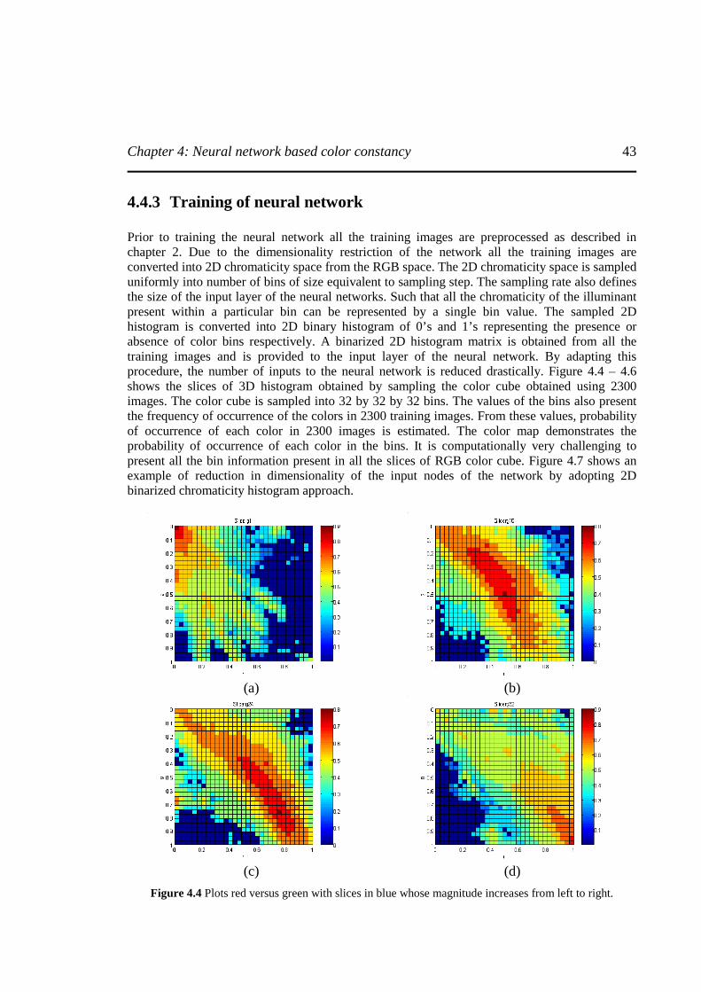
Chapter 4: Neural network based color constancy
43
4.4.3 Training of neural network Prior to training the neural network all the training images are preprocessed as described in chapter 2. Due to the dimensionality restriction of the network all the training images are converted into 2D chromaticity space from the RGB space. The 2D chromaticity space is sampled uniformly into number of bins of size equivalent to sampling step. The sampling rate also defines the size of the input layer of the neural networks. Such that all the chromaticity of the illuminant present within a particular bin can be represented by a single bin value. The sampled 2D histogram is converted into 2D binary histogram of 0’s and 1’s representing the presence or absence of color bins respectively. A binarized 2D histogram matrix is obtained from all the training images and is provided to the input layer of the neural network. By adapting this procedure, the number of inputs to the neural network is reduced drastically. Figure 4.4 – 4.6 shows the slices of 3D histogram obtained by sampling the color cube obtained using 2300 images. The color cube is sampled into 32 by 32 by 32 bins. The values of the bins also present the frequency of occurrence of the colors in 2300 training images. From these values, probability of occurrence of each color in 2300 images is estimated. The color map demonstrates the probability of occurrence of each color in the bins. It is computationally very challenging to present all the bin information present in all the slices of RGB color cube. Figure 4.7 shows an example of reduction in dimensionality of the input nodes of the network by adopting 2D binarized chromaticity histogram approach.
(a) (b)
(c) (d)
Figure 4.4 Plots red versus green with slices in blue whose magnitude increases from left to right.
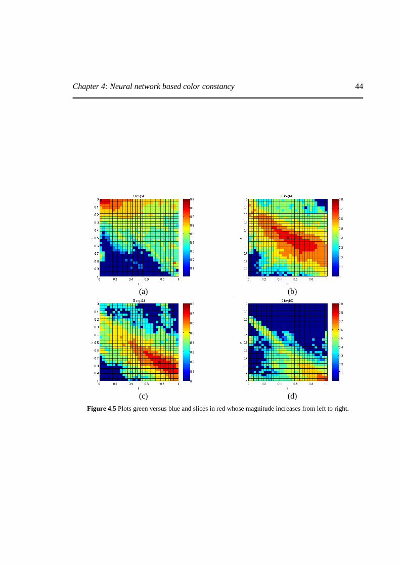
Chapter 4: Neural network based color constancy
44
(a) (b)
(c) (d)
Figure 4.5 Plots green versus blue and slices in red whose magnitude increases from left to right.
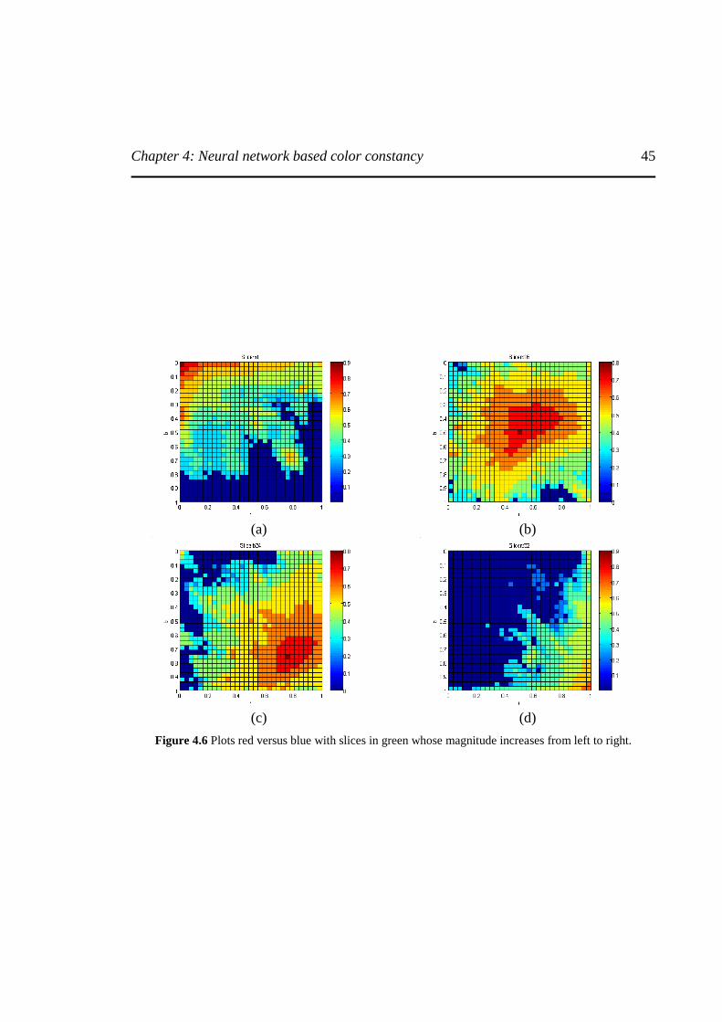
Chapter 4: Neural network based color constancy
45
(a) (b)
(c) (d)
Figure 4.6 Plots red versus blue with slices in green whose magnitude increases from left to right.
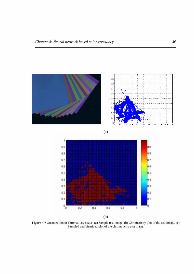
Chapter 4: Neural network based color constancy
46
(a)
(b)
Figure 4.7 Quantization of chromaticity space. (a) Sample test image, (b) Chromaticity plot of the test image. (c) Sampled and binarized plot of the chromaticity plot in (a).
Chapter 4: Neural network based color constancy
47
Based on the example presented in figure 4.7, drastic reduction in the size of the input to the neural network is recorded. The chromaticity plot in figure 4.8 (a) consists of 74,000 points. After sampling at sampling rate of 45, i.e., 2025 bins, 74,000 points are reduced to 2025 points, out of which 467 bins only contain the chromaticity values of the illuminant. These are labeled as 1’s (active bins) and rests are labeled 0’s (inactive bins). Thus only active bins containing the information about the illuminant chromaticity are presented to the network. Based on the input to the neural network, its architecture is designed. Appropriate selection of numbers of hidden layers and number of neurons in hidden layers is essential. We initially experimented with one hidden layer with 10 neurons. Figure 4.8 show the network architecture. Conjugate gradient training algorithm is used to train the network. However different there are different regularization training algorithms are available to obtain a regularized solution. They are
1. Bayesian regularization algorithm. 2. Weight decay algorithm. 3. Cross validation algorithm.
There are two reasons for not using these algorithms for training the neural network in our case. First, these regularized training algorithms require large memory and second none of these algorithms have been proven to provide better estimates of the neural network output.
4.4.4 Testing neural network Once the neural network is trained properly for a given sample of training images, the network is tested on set of test images which network has never seen before. The test images / image is presented to the trained neural network in similar fashion as all the training images where presented, i.e., the 3D RGB color space of test images / image is converted into 2D chromaticity space. The chromaticity space is sampled using same sampling rate into 2D chromaticity histogram which is binarized into 0’s and 1’s representing active and inactive bins of test images. Trained neural network estimates the chromaticity of the test images / image. Given the estimate of the test image chromaticity value, it is corrected using the diagonal transformation model [Finlayson’94b]. After applying the diagonal transformation, the intensity of the image is adjusted such that the average intensity of the image is constant. The average intensity is computed both before and after the diagonal transformation.
4.5 Limitations of neural network Universal approximator – Neural network has number of limitation that affects the performance of the neural network drastically. Following list is what is known as ‘curses of neural networks’
1. Random Initialization of weight values: The value of weights assigned to the connection between the input, hidden layers and the output layer is initialized in random
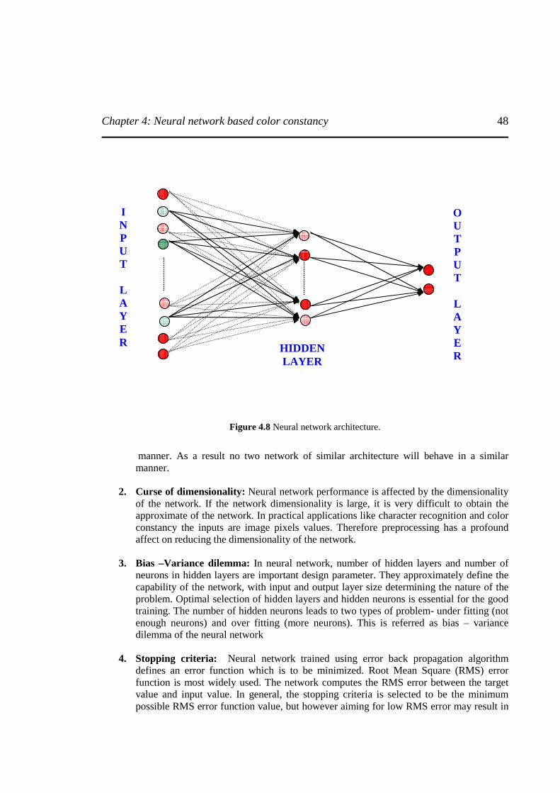
Chapter 4: Neural network based color constancy
48
Figure 4.8 Neural network architecture.
manner. As a result no two network of similar architecture will behave in a similar manner.
2. Curse of dimensionality: Neural network performance is affected by the dimensionality
of the network. If the network dimensionality is large, it is very difficult to obtain the approximate of the network. In practical applications like character recognition and color constancy the inputs are image pixels values. Therefore preprocessing has a profound affect on reducing the dimensionality of the network.
3. Bias –Variance dilemma: In neural network, number of hidden layers and number of
neurons in hidden layers are important design parameter. They approximately define the capability of the network, with input and output layer size determining the nature of the problem. Optimal selection of hidden layers and hidden neurons is essential for the good training. The number of hidden neurons leads to two types of problem- under fitting (not enough neurons) and over fitting (more neurons). This is referred as bias – variance dilemma of the neural network
4. Stopping criteria: Neural network trained using error back propagation algorithm
defines an error function which is to be minimized. Root Mean Square (RMS) error function is most widely used. The network computes the RMS error between the target value and input value. In general, the stopping criteria is selected to be the minimum possible RMS error function value, but however aiming for low RMS error may result in
I N P U T
L A Y E R
O U T P U T
L A Y E R
HIDDEN LAYER

Chapter 4: Neural network based color constancy
49
over fitting and aiming low RMS error may result in under fitting. Therefore it is important to make proper selection of stopping criteria.
5. Learning rate: The training time of the neural network is also an important issue.
Network with large architecture generally takes more training time. However this issue can be handled by adapting different learning rates. Unfortunately, optimal selection of learning rate is not defined. Therefore, if large learning rate is selected then network will learn nothing because gradient jump will be large and it will converge quickly with little training. On the other hand, if the learning rate is small, we run in to risk of getting struck in local minima’s.
Summing up the limitation of the neural network, it can be concluded that neural network is highly unstable universal approximator and very difficult to regularize.
Chapter 5: Support vector machine based color constancy
50
Chapter 5
5 SUPPORT VECTOR MACHINE BASED COLOR CONSTANCY This chapter opens the discussion on new learning theory based approach for color constancy. This approach is more stable and provides global solution unlike neural networks. Different aspects of the theory like quantitative analysis, loss functions, applications to linear and nonlinear data sets and extension to color constancy is discussed. It is one of the contribution of this thesis work. The limitation of statistical techniques to develop an empirical data model related to many engineering applications led to the advent of relatively new theory of functional estimation in regression and classification in the form of Support Vector Machine (SVM). The theory is derived from the statistical learning theory developed by Vapnik and Chervonenkis [Vapnik’97]. The empirical data modeling is based on the induction principle, where the model infers information from the data presented to it and later tries to predict it for the data set it has never seen similar to neural networks. Due to restriction such as finite data’s and the high dimensional nature of the problem the data will form only a sparse distribution in the input space. Therefore it is an ill-posed problem. SVM is a novel learning theory based on the framework of Structural Risk Minimization (SRM) unlike traditional neural network that is based on the Expected Risk Minimization (ERM) principle. Traditional neural network approaches have suffered difficulties with generalization, producing models that can over fit the data. This is a consequence of the optimization algorithms used for parameter selection and the statistical measures used to select the ‘best’ model. SVM developed for classification problem is also extended to the functional estimation regression problem [Vapnik’97]. The mathematical foundation and superior performance of SVM over traditional neural network, presents an exciting alternative to neural network based color constancy. The subsection 5.1 presents foreword towards supports vector machines for regression (SVR) in linear and nonlinear domain. The forms of loss functions used in SVR are outlined. The subsection 5.2 is on the optimization of the free parameters and finally SVR for color constancy is discussed in subsection 5.3.
5.1 Support Vector Machines for Regression The support vector machines designed initially for classification is extended to regression problems by introducing different loss functions. Suppose provided with a given set of data points, represented by vectorx , the SVM learns the functional dependency between the input and output. It is given by )(xf . Equation (5.1) presents simple expression for SVM learned dependency for regression problem.

Chapter 5: Support vector machine based color constancy
51
)(),(1
xwwxfN
iiϕ∑
=
=
(5.1)
where the functions )(xϕ are called the feature function. The term iw corresponds to the weights
assigned to each of the input data points. In regression, some sort of error approximation is used to obtain the best functional estimation between the input and output data points. These error measures are defined as loss functions.
5.1.1 Loss functions The extension of SVM from classification to regression problem is based on alternative loss functions or error approximation measures. There is four possible loss function used in general applications.
1. Quadratic loss function 2. Absolute loss function 3. Huber loss function 4. ε -insensitive loss function
The loss functions are shown in figure 5.1. Quadratic and Huber loss function shown in figure 5.1(a) and (c) are classical error functions given by square error or L2 norm. Application of Huber error function results in robust regression analysis and it is very useful if nothing specific is available about the model of noise. The absolute error shown in figure 5.1(b) is given by the L1 norm. This error function is insensitive to outliers. However, all the three error function produced no sparseness in support vectors. Therefore Vapnik introduced ε -insensitive loss function, shown in figure 5.1(d) that will enable sparse sets of the support vectors to be obtained. The ε -insensitive loss function is expressed mathematically in equation (5.2). If the difference between the predicted and measured value is withinε , then error is zero, otherwise it is the magnitude of the difference between the predicted value and the radius ε of the tube. At ε =0, it is equivalent to least modulus function.
( ) ( )( )
−−≤−
=−otherwisewxfy
wxfyifwxfy
εε
ε ,
, 0 ,
(5.2)
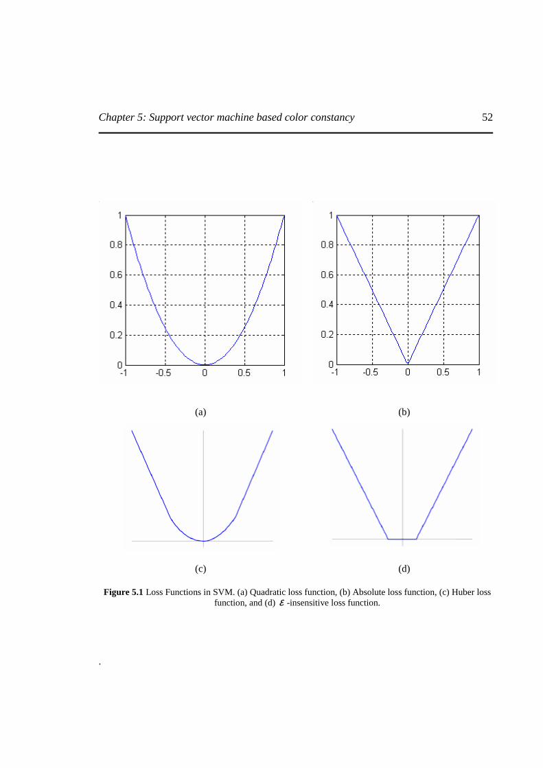
Chapter 5: Support vector machine based color constancy
52
.
(a) (b)
(c) (d)
Figure 5.1 Loss Functions in SVM. (a) Quadratic loss function, (b) Absolute loss function, (c) Huber loss function, and (d) ε -insensitive loss function.
Chapter 5: Support vector machine based color constancy
53
5.1.2 Linear regression The support vector machines is initially applied and tested for linear regression. In order to perform linear regression, a cost function is defined. The objective is to minimize the cost function, thus estimating a linear regression hyperplane ),( wxf by minimizing equation (5.3),
( ) λε
/1~C , C2
1
1,
2
−+= ∑
=
l
iii wxfywR
(5.3)
In order to minimize equation (5.3), slack variables ( ∗ξξ and ) are introduced. The slack variables are variables outside the tube present on the either side of the tube of thicknessε . Slack
variables are positive integer values. Lagrangian multiplier ( ∗ii αα and ) is used for minimization
of cost function. The values of lagrangian multipliers are zero if the slack variables are within the tube and it is nonzero if the slack variables are outside the tube. These nonzero lagrangian multipliers are the support vectors. The cost function is modified into equation (5.4).
∗
∗
= =
∗
+≤−
+≤−
=≥
++= ∑ ∑
ξεξε
ξξξξ
iiT
iT
i
l
i
l
i
yxw
xwy
liwR ,1,0),( ,C2
1
1 1
2
(5.4)
The constant C is the regularization parameter which controls the trade-off between the
approximation error and the weights vector normw . The constrained specified in equation (5.4),
is solved by solving the primal variables Lagrangian( )∗∗∗ ββααξξ ,,,,,,,bwL ip . The primal
variables lagrangian has to be minimized with respect to ∗ξξ ,,,bwi and maximized with respect
to non-negative lagrangian multipliers ∗∗ ββαα ,,, . Therefore cost function is solved either in primal space or in dual space. A solution in dual space is selected. The dual variables lagrangian
( )∗αα ,dL is expressed in terms of Lagrange multipliers only. There are 2l multipliers for linear
regression, and the Hessian matrix H for optimization is of size (2l, 2l) matrix. Thus dual variable lagrangian is optimized as expressed in equation (5.5),
ααα TTd fHL +−= 5.0 (5.5)
After calculating the Lagrangian multipliers ∗ii αα and , the optimal weights and bias vector for
regression hyperplane is computed using the expression in equation (5.6) and (5.7),
( ) i
l
iiio xw ∑
=
∗ −=1
αα
(5.6)
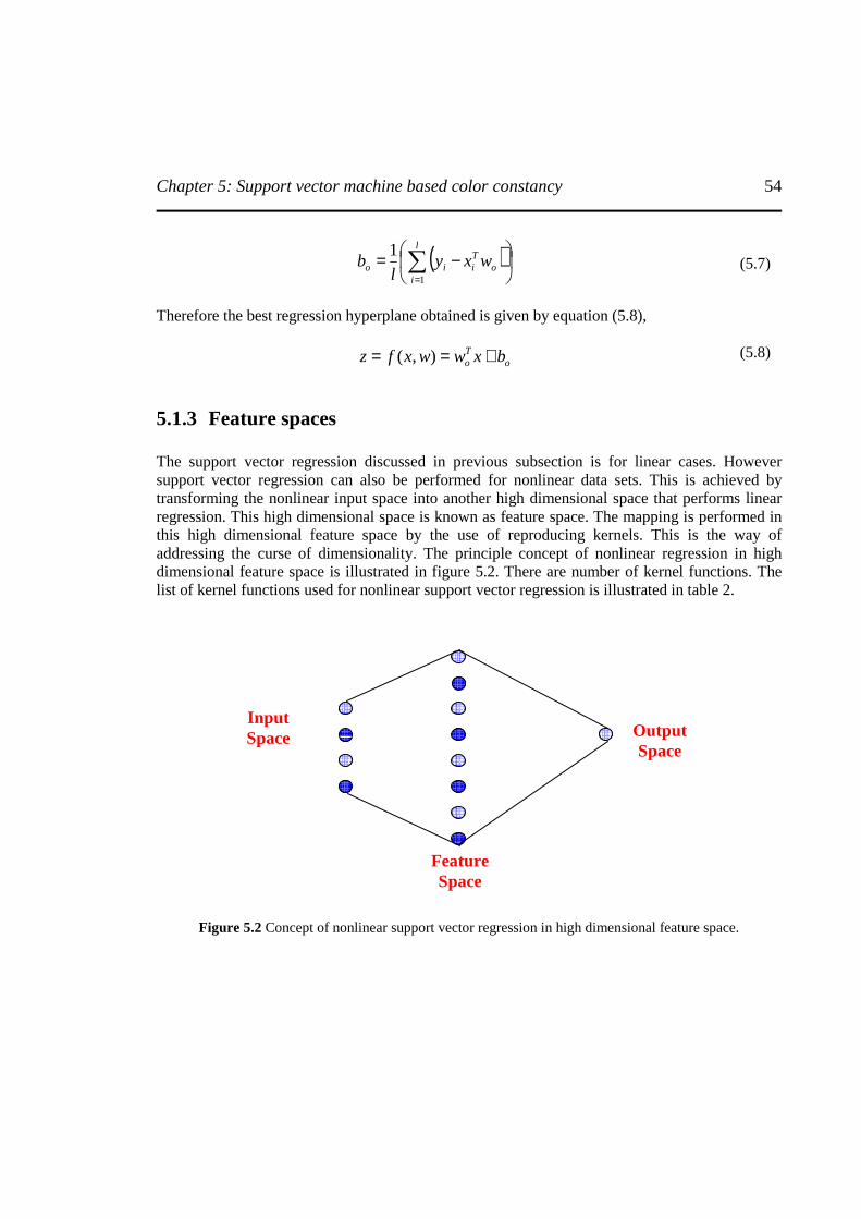
Chapter 5: Support vector machine based color constancy
54
( )
−= ∑=
l
io
Tiio wxy
lb
1
1
(5.7)
Therefore the best regression hyperplane obtained is given by equation (5.8),
oTo bxwwxfz +== ),( (5.8)
5.1.3 Feature spaces The support vector regression discussed in previous subsection is for linear cases. However support vector regression can also be performed for nonlinear data sets. This is achieved by transforming the nonlinear input space into another high dimensional space that performs linear regression. This high dimensional space is known as feature space. The mapping is performed in this high dimensional feature space by the use of reproducing kernels. This is the way of addressing the curse of dimensionality. The principle concept of nonlinear regression in high dimensional feature space is illustrated in figure 5.2. There are number of kernel functions. The list of kernel functions used for nonlinear support vector regression is illustrated in table 2.
Figure 5.2 Concept of nonlinear support vector regression in high dimensional feature space.
Input Space Output
Space
Feature Space

Chapter 5: Support vector machine based color constancy
55
Table 5.1 Kernel functions for nonlinear support vector regression.
Kernel Function Formulation Polynomial kernel d
xxxxK ′=′ ,),(
Gaussian Radial Basis Function
′−−=′
2
2
2exp),(
σxx
xxK
Exponential Radial Basis Function
′−−=′
22exp),(
σxx
xxK
Multilayer Perceptron ( )φυ +′=′ xxxxK ,tanh),(
Fourier Series ( )
( )
′−
′−
+=′
xx
xxNxxK
21
sin
21
sin),(
Spline ( ) ( )k
s
kN
ss
k
r
rr xxxxxxK ++==
−′−+=′ ∑∑ ττ10
'),(
B- Spline ( )xxBxxK N ′−=′ +12),(
Additive Kernel ( )xxKxxKi
i ′=′ ∑ ,),(
Tensor product ( )∏ ′=′i
i xxKxxK ,),(
With so many kernel functions at disposal, the choice of best kernel is important. However it is not easy to answer. But with so many functions, one can experiment. However unless strong theoretical explanation is established for selection of kernel, cross validation will remain as an effective method for selection of kernel.
5.1.4 Nonlinear regression SVR for nonlinear case is performed in high dimensional feature space using appropriate kernel function selected from the table 5.1. Similar to linear regression, the cost function is optimized in dual space, i.e., dual variable lagrangian maximized with respected to lagrangian multipliers. The solution for a regression hyperplane )(xf which is linear in feature space F will create a nonlinear regression hyperplane in the original input space. The nonlinear regression function at a given point is expressed in equation (5.9),
( ) ( ) bxxKxf iSVs
ii +−=∑ ∗ , )( αα (5.9)

Chapter 5: Support vector machine based color constancy
56
In the case of nonlinear regression, the Hessian matrix is changed, expressed in equation (5.10),
( )ik xxGGG
GGH , ,
−−
=
(5.10)
After calculating the lagrangian multipliers, the optimal desired weight vectors and bias vectors are calculated using the equation (5.11) and (5.12),
αα −= ∗ow
(5.11)
( )
−= ∑=
l
ioio Gwy
lb
1
1
(5.12)
Thus the best nonlinear regression hyperplane is given by equation (5.13),
oo bGwwxfz +== ),( (5.13)
5.2 Selection of free parameters Support vector machine for nonlinear / linear regression has two free parameters namely, ε -epsilon and constant C -regularization parameter. To obtain optimal regression hyperplane in linear or nonlinear cases, these two parameters are to be optimized. However in the case of nonlinear regression, Gaussian RBF kernel is most commonly used. Gaussian RBF kernel has one free parameter namely, σ -sigma. Therefore all the three free parameters are to be optimized. Analyzing the influence of all the three parameters [Mattera’99] shows that the choice of ε affect the approximation error, training time and the complexity of the solution. For the choice ofC , small value of C results in poor approximation and large Ccauses numerical instability. Appropriate selection of σ is essential for proper reconstruction of the model. There is no theoretical perfect method for optimal selection of any of the parameter. But cross validation technique is used for optimal selection of the free parameters. In linear regression, cross validation can be performed over a grid of values of ε andC . In nonlinear regression, cross validation is performed over a grid of values of C and σ for a constant value ofε . After optimal estimation of Candσ , the support vector regression is performed at different. Thus cross validation provides an option to select optimal values for the free parameters. However, sometimes cross validation fails, resulting in overfitting and inaccurate data model.
Chapter 5: Support vector machine based color constancy
57
5.3 Support Vector Regression for color constancy The advantages of SVR over traditional neural network encouraged to evaluate the application of SVR to solve for color constancy. SVR like neural network involves ‘Training’ and ‘Testing’ phase. The procedure adopted to present input matrix and target values for the training data set is similar to the one adopted for neural network. i.e., data generation using bootstrapping algorithm, GW / SBM estimate of the target values, 3D space to 2D space transformation, uniform sampling and binarized 2D histogram. Unlike neural network, SVR does not face input dimensionality problem, so the dimensionality of the input matrix is immaterial. But SVR have only single output, therefore SVR has to be performed on each chromaticity channels individually. In each training process, three free parameters are to be optimized. Therefore 6 times optimization of the free parameters has to be performed. This it is a cumbersome process with large training data set. In case of 3D space the same process has to be performed 9 times, increasing the computational expense. Therefore we perform SVR color constancy in 2D space to reduce the computational expensiveness.
5.3.1 Training support vector machine Training support vector machine involves two separate training for ‘r’ and ‘g’ chromaticity respectively. Solving SVM requires quadratic optimization. Though SVM is independent of input dimensionality, the quadratic optimization is dependent on the number of input data set, i.e., size of the optimization problem depends on the number of training data sets. Suppose n is the size of
the training data set, the optimization matrix size will be2n requiring order of 2n memory and time resources to train. Therefore training for large value of n makes impossible to optimization matrix to keep in memory. Similar problem is faced when training for 2300 training images. One approach to make the training of SVM possible on problems with many training images tractable is to decompose the problem into series of smaller tasks. In literature many approaches has been suggested to speed up the training of SVM by decomposing the optimization matrix like SVMlight [Joachims’99], Nodelib [Flake’00], [Lin’00], Sequential Minimization Optimization (SMO) [Platt’99], and SVMTorch [Collobert’01]. In this thesis work, we use SVMTorch1
[Collobert’01] to fasten the training process and avoid memory issues. SVMTorch decomposes the optimization matrix based on the decomposition algorithm of Osuna et al. [Osuna’97]. The SVMTorch developed for classification, is modified to solve for the regression problems. During the training phase, the free parameters are optimized using a cross validation technique. We split the training data into two – Training data and Validation data. The SVM is trained over a grid of values of free parameter using training data and tested on the validation data. The combination of free parameters at which the estimation of chromaticity for the validation data produces least RMS error is selected. 1. SVMTorch is available at htt://www.idiap.ch/learning/SVMTorch.html.
Chapter 5: Support vector machine based color constancy
58
5.3.2 Testing support vector machine Once SVM is trained properly using SVMTorch algorithm, the performance of the trained SVM is tested on testing data set in estimating the chromaticity of the illuminant. A 2D binarized testing matrix of test image or images of 1’s and 0’s representing the presence and absence of chromaticity in the images or images is provided to a learned SVM. The estimate of the chromaticity of the illuminant is obtained for the test images. Once the estimate is obtained linear diagonal transformation [Finlayson’96b] is applied to obtain a color corrected image. The intensity of the color corrected in adjusted both before and after applying linear diagonal transformation. The efficiency of the estimation is obtained by computing the error between the estimated chromaticity value and the true chromaticity value. In case of uncalibrated data where true chromaticity estimate is not available, visual judgment of the color corrected image is used as measure of efficiency of the algorithm.
Chapter 6: Ridge regression based color constancy
59
Chapter 6
6 RIDGE REGRESSION BASED COLOR CONSTANCY In this chapter, application of linear least squares and ridge regression to solve for color constancy is presented. These are linear modeling techniques used to investigate the relationship between two variables, i.e., summarizes the straight line dependence between one variable on another. Ordinary least square (OLS) is a technique that minimizes the distance (sum of the squares of the error term) between the observed (true) values and the predicted (estimated) value. If the inputs are correlated, the model coefficients of the OLS is zero, so value cannot be predicted, therefore a regularization parameter is added to the OLS solution, to estimate the model coefficients. Based on the previous discussion on the relationship between the chromaticity of the illuminant and the digital image formation, variation in the chromaticity of the illuminant causes corresponding change in the appearance of the image. We study this transformation using a linear modeling technique assuming constant surface reflectance and sensor characteristics. The advantage of these approaches is that they are simple, fast and analytically solvable. OLS can handle large dimensional input matrix with easy unlike its sophisticated counterpart’s neural network and support vector machines. This section is outlined as follows: Subsection 6.1 presents discussion of the assumption of ordinary least squares and presents its analytical solution. Subsection 6.2 presents extension of ordinary least squares into a regularized approach ‘ridge regression’ and its analytical derivation. Subsection 6.3 presents cross validation technique to estimate the free parameterλ . Subsection 6.4 presents application of ridge regression in estimating the chromaticity of the illuminant and solve for color constancy.
6.1 Ordinary Least Squares Ordinary least square technique is an unbiased linear estimation technique of the training data that are linearly related. It also has the smallest variance among the unbiased estimators. However, the following is true under certain assumptions. Following are the assumptions under which OLS produces best linear unbiased estimators.
1. There is no correlation between input variables and residual. 2. The expected value of the residuals equals zero. 3. Residuals are homoskedastic. 4. Input variables are independent. 5. Input variables are measured with no error, i.e., input matrix is has zero error.

Chapter 6: Ridge regression based color constancy
60
Violation of any one of the assumptions mentioned above, leads to a biased estimator. In practical cases, it is very difficult to satisfy the above assumptions especially the assumptions 5. We now present analytical solution for OLS abiding with all the above assumptions. The OLS estimation of a linear training data ( ) ( ) ( )nn yxyxyx ,,.....,,,, 2211 of d dimension is given by expression in equation (6.1),
( ) XWxfY == (6.1)
( ) Td
d
jjj XwwwwxwwY ,....,, 210
10 +=+= ∑
=
(6.2)
where ( )dwwW ,......,0= are the model coefficients. The noise η of zero mean and 2σ variance is added to equation (6.1) to get equation (6.3)
η+= YY (6.3)
In OLS regression, the model coefficients are obtained to minimize the error metric between the observed and predicted values. Therefore sum of the square error from the true value is given in equation (6.4)
( ) ( )
( ) ( )XWYXWY
xwwY
YYS
T
n
i
d
jijji
n
iii
n
i
-ˆ-ˆ
ˆ
ˆ
2
1 10
1
2
1
2
=
−−=
−==
∑ ∑
∑∑
= =
==
η
(6.4)
where ( )321 ˆˆˆˆ y,,.........y,yY = and
=
ndn
d
xx
xx
X
..1
.....
.....
..1
1
111
The error is a quadratic function and can be solved by differentiating with respect to W and equating to zero.
( ) 0ˆ2 =−=∂∂
-XWYXW
Tη
(6.5)
Chapter 6: Ridge regression based color constancy
61
If X is nonsingular,( ) 1−XX T exists,
( ) 0ˆ =-XWYX T (6.6)
Solving forW , gives equation (6.7) which are the model coefficients,
( ) YXXXW TT ˆ1−= (6.7)
The predicted model output for the training data is given by equation (6.8)
( ) YXXXXY TT ˆ1−= (6.8)
6.2 Ridge regression Ridge regression also known as regularized least square methods is a technique intended to overcome ‘ill-conditioned’ situation. The ill-condition occurs when the correlation between the
input matrix is high, which implies that ( ) 1 −XX T is a rank deficient, giving rise to unstable parameter estimates, typically with large standard errors. Therefore, in ridge regression, additional information is added to remove the ill-conditioning. From Bayesian perspective, it is
similar to placing a prior knowledge about the model coefficient of the form ),0(~ 1−λNW and computing the mode of posterior. The analytical solution of the ridge regression is presented below. The ridge model of a linear training data is obtained by minimizing equation (6.9)
( ) ∑=
+−=d
j
WYY1
22ˆ λη
(6.9)
Comparing equation (6.4) and (6.9), one can notice that prior information about the model coefficient is added to original OLS model estimation. Here λ is a regularization parameter, which controls the trade-off between the residual error and the regularized solution. Solving analytically equation (6.9) to obtain ridge model coefficient, the error of sum of the square from the true value is given in equation (6.10),
( )
( ) ( ) WWXWYXWY
WxwwY
WYYS
TT
d
jj
n
i
d
jijji
d
jj
n
iii
n
iridge
λ
λ
λη
+−−=
−
−−=
−−==
∑∑ ∑
∑∑∑
== =
===
ˆˆ
ˆ
)ˆ(
1
2
1
2
10
1
2
1
2
1
2
(6.10)
Chapter 6: Ridge regression based color constancy
62
The equation (6.10) is equivalent to optimization problem:
0, subject to
ˆminarg
1
2
1 10
>≤
−−=
∑
∑ ∑
=
= =
d
jj
n
i
d
jijji
Wridge
ssw
xwwYW
(6.11)
Differentiating equation (6.10) w.r.t W and equating it to zero, we get ridge model coefficients in equation (6.14)
( ) ( ){ }W
WWXWYXWY
W
S TTridge
∂+−−∂=
∂∂ ˆˆ λ
(6.12)
( ) 0 2ˆ2 =++−=∂
∂WIXXYX
W
S TTridge λ
(6.13)
( ) YXIXXW TTridge
ˆ1−+= λ (6.14)
where I is a identity matrix of dimensiond . From equation (6.14), it is noted that the first factor
( )IXX T λ+ is always invertible because a small positive diagonal matrix is added. The ridge predicted value of the training data is given by equation (6.15).
( ) YXIXXXY TTridge
ˆ1−+= λ (6.15)
6.3 Cross Validation selection of The regularization parameter λ controls the trade-off between the residual error and the regularized solution. Optimal selection of λ is essential because large value of λ results in an under fitting and small value of λ results in overfitting. Therefore it is important to choosee right value of the regularization parameter. There are number of methods for the selection of regularization parameter.
1. Trail and error method 2. Generalized Cross Validation (GCV) 3. L-curve 4. Cross Validation
In this work, Cross validation method to used to select optimal lambda. The reason for choosing cross validation is because both generalized cross validation and L-curve methods failed to provide optimal choice of lambda. The lambda selected by both GCV and L-curve method provided under fitted training data model. The reason for the failure of GCV and L-curve may be
Chapter 6: Ridge regression based color constancy
63
associated with ill-conditioned nature of the training matrix. Therefore we selected cross validation over trail and error method. In cross validation method, the training data is split into two: Training data and the validation data. The cross validation is performed on the former sets of data for a vector of lambda values and validation error is computed over validation set of data. The value of lambda for which the validation error is minimum for a given lambda is selected.
6.4 Ridge regression for color constancy Ridge regression for color constancy is performed in the chromaticity space. It has two stages; training and testing stages. In the training stage, all the training data set is converted into chromaticity space, sampled and binarized to obtain a 2D binary histogram in accordance with works of Cardei and Funt [Funt’99]. In practical application, it is difficult to measure the chromaticity of the illuminant so gray world estimate of the observed images is used as target values. The training data set consists of more than 2300 images. Therefore the dimensionality of the input matrix X is 2300 x N, where N is the number of sampled bins. Based on the analytical discussion above the ridge model coefficients are computed for the training input matrix. Cross validation discussed above is used to select the lambda value. The estimated ridge model coefficient is then used to estimate the chromaticity value of the validation data set. The error between the estimated chromaticity values and the observed chromaticity values is a function of lambda. Therefore optimal lambda value at which validation error is smallest provides the best possible ridge model prediction of the chromaticity of the training input matrix. In the testing phase, the test matrix is presented to the ridge coefficients in a similar fashion as presented during the training phase. The chromaticity of the illuminant is estimated for the test data set. After the chromaticity estimation, the chromaticity space is converted back to 3D RGB space. Linear diagonal transformation is applied to color correct the image.
Chapter 7: Comparison of color constancy algorithms
64
Chapter 7
7 COMPARISON OF COLOR CONSTANCY ALGORITHMS In this chapter, we present the performance evaluation of color constancy algorithms on both the calibrated and uncalibrated images. The performance evaluation is performed in both the quantitative and qualitative domain. Root mean square (RMS) error measure is used for quantitative evaluation. A discussion is provided at the end on the computational and algorithmic complexities of the algorithms. The chapter is outlined as follows: Subsection 7.1 presents the evaluation of the algorithms on the calibrated image dataset. Subsection 7.2 presents evaluation of the algorithm on the uncalibrated images, and finally summary on the results is provided in subsection 7.3.
7.1 Algorithm performance for calibrated real images In this thesis, term calibrated real images refers to the publicly available image dataset [Barnard’02c], generated under controlled illumination varying conditions and true R, G, and B values of the illuminant used is known. The test image dataset consists of 30 different images captured under 11 different illuminants. The chromaticities of the 11 illuminant used to generate test image data set is presented in figure 7.1. The chromaticities of the training dataset of images using gray world algorithm is presented in figure 7.2. The baseline description of the learning theory algorithm involves following steps.
1. Preprocess both the training and test images. 2. Convert all the training and test images into 2D chromaticity space. 3. Uniformly sample the chromaticity space into N bins. 4. Convert the sampled chromaticity space into 2D binary histogram with 1’s representing
presence of chromaticity and 0’s representing no chromaticity values. 5. Generate an approximate estimate of target chromaticity values of training images using
gray world algorithm. 6. An individual trained model is generated from a 2D binarized training histogram for each
of the learning theory algorithm. Parameter optimization is performed using cross validation.
7. To this trained model, 2D test histogram is presented to obtain the chromaticity estimation.
8. Linear diagonal transformation is performed after the chromaticity values are estimated. All the results presented in this chapter are generated by following the above mentioned steps.
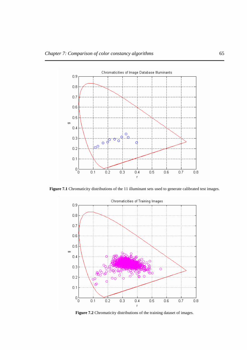
Chapter 7: Comparison of color constancy algorithms
65
Figure 7.1 Chromaticity distributions of the 11 illuminant sets used to generate calibrated test images.
Figure 7.2 Chromaticity distributions of the training dataset of images.
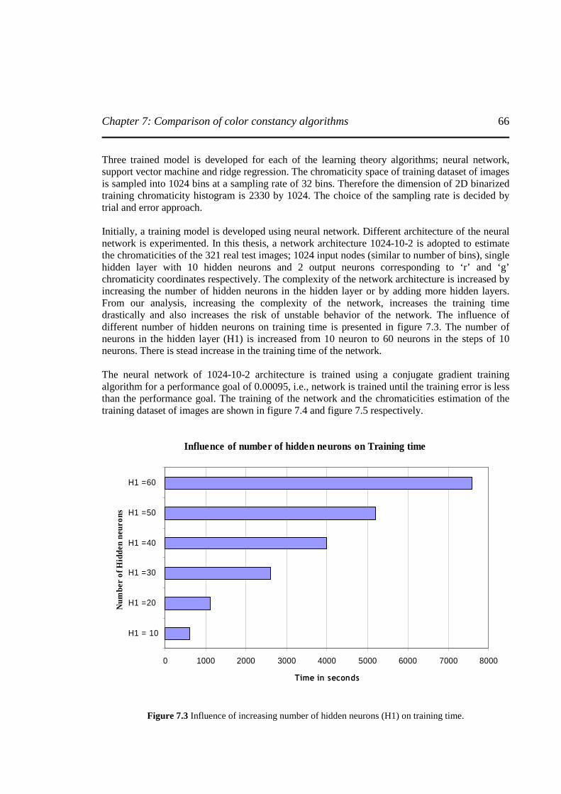
Chapter 7: Comparison of color constancy algorithms
66
Three trained model is developed for each of the learning theory algorithms; neural network, support vector machine and ridge regression. The chromaticity space of training dataset of images is sampled into 1024 bins at a sampling rate of 32 bins. Therefore the dimension of 2D binarized training chromaticity histogram is 2330 by 1024. The choice of the sampling rate is decided by trial and error approach. Initially, a training model is developed using neural network. Different architecture of the neural network is experimented. In this thesis, a network architecture 1024-10-2 is adopted to estimate the chromaticities of the 321 real test images; 1024 input nodes (similar to number of bins), single hidden layer with 10 hidden neurons and 2 output neurons corresponding to ‘r’ and ‘g’ chromaticity coordinates respectively. The complexity of the network architecture is increased by increasing the number of hidden neurons in the hidden layer or by adding more hidden layers. From our analysis, increasing the complexity of the network, increases the training time drastically and also increases the risk of unstable behavior of the network. The influence of different number of hidden neurons on training time is presented in figure 7.3. The number of neurons in the hidden layer (H1) is increased from 10 neuron to 60 neurons in the steps of 10 neurons. There is stead increase in the training time of the network. The neural network of 1024-10-2 architecture is trained using a conjugate gradient training algorithm for a performance goal of 0.00095, i.e., network is trained until the training error is less than the performance goal. The training of the network and the chromaticities estimation of the training dataset of images are shown in figure 7.4 and figure 7.5 respectively.
Influence of number of hidden neurons on Training time
0 1000 2000 3000 4000 5000 6000 7000 8000
H1 = 10
H1 =20
H1 =30
H1 =40
H1 =50
H1 =60
Num
ber
of H
idde
n ne
uro
ns
Time in seconds
Figure 7.3 Influence of increasing number of hidden neurons (H1) on training time.
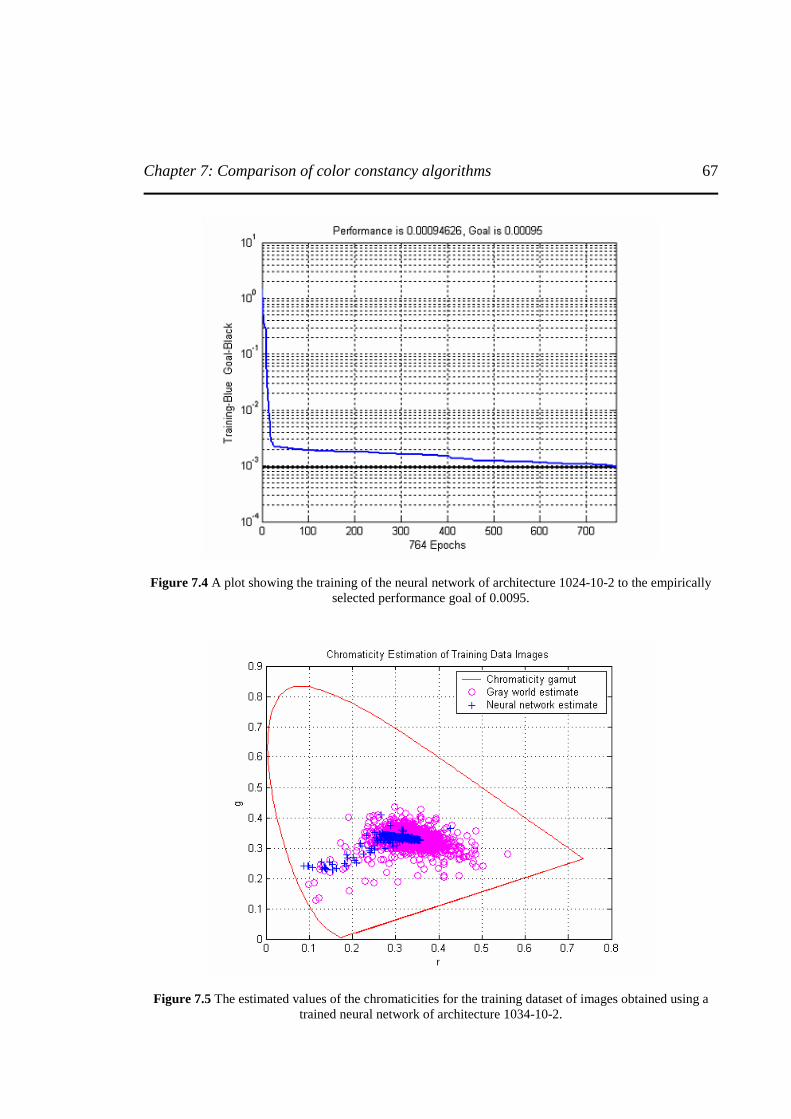
Chapter 7: Comparison of color constancy algorithms
67
Figure 7.4 A plot showing the training of the neural network of architecture 1024-10-2 to the empirically selected performance goal of 0.0095.
Figure 7.5 The estimated values of the chromaticities for the training dataset of images obtained using a trained neural network of architecture 1034-10-2.
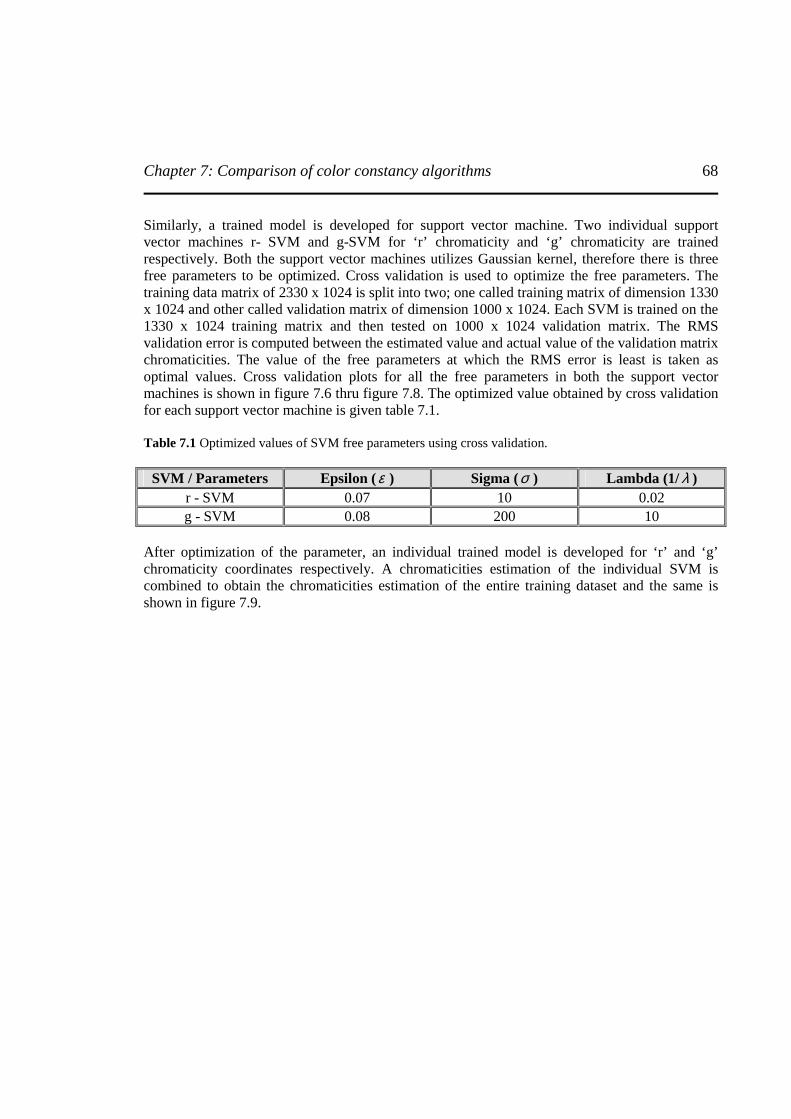
Chapter 7: Comparison of color constancy algorithms
68
Similarly, a trained model is developed for support vector machine. Two individual support vector machines r- SVM and g-SVM for ‘r’ chromaticity and ‘g’ chromaticity are trained respectively. Both the support vector machines utilizes Gaussian kernel, therefore there is three free parameters to be optimized. Cross validation is used to optimize the free parameters. The training data matrix of 2330 x 1024 is split into two; one called training matrix of dimension 1330 x 1024 and other called validation matrix of dimension 1000 x 1024. Each SVM is trained on the 1330 x 1024 training matrix and then tested on 1000 x 1024 validation matrix. The RMS validation error is computed between the estimated value and actual value of the validation matrix chromaticities. The value of the free parameters at which the RMS error is least is taken as optimal values. Cross validation plots for all the free parameters in both the support vector machines is shown in figure 7.6 thru figure 7.8. The optimized value obtained by cross validation for each support vector machine is given table 7.1. Table 7.1 Optimized values of SVM free parameters using cross validation. SVM / Parameters Epsilon (ε ) Sigma (σ ) Lambda (1/λ )
r - SVM 0.07 10 0.02 g - SVM 0.08 200 10
After optimization of the parameter, an individual trained model is developed for ‘r’ and ‘g’ chromaticity coordinates respectively. A chromaticities estimation of the individual SVM is combined to obtain the chromaticities estimation of the entire training dataset and the same is shown in figure 7.9.
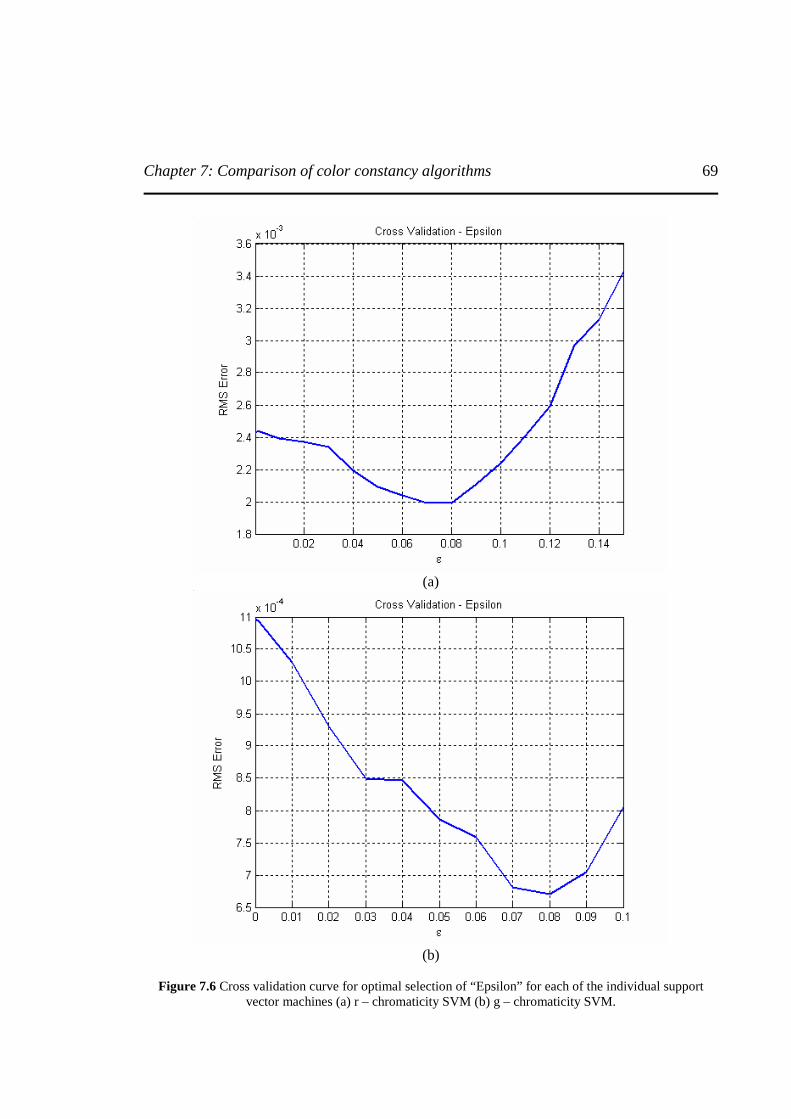
Chapter 7: Comparison of color constancy algorithms
69
(a)
(b)
Figure 7.6 Cross validation curve for optimal selection of “Epsilon” for each of the individual support
vector machines (a) r – chromaticity SVM (b) g – chromaticity SVM.

Chapter 7: Comparison of color constancy algorithms
70
(a)
(b)
Figure 7.7 Cross validation curve for optimal selection of “Sigma” for each of the individual support
vector machine (a) r – chromaticity SVM (b) g – chromaticity SVM.
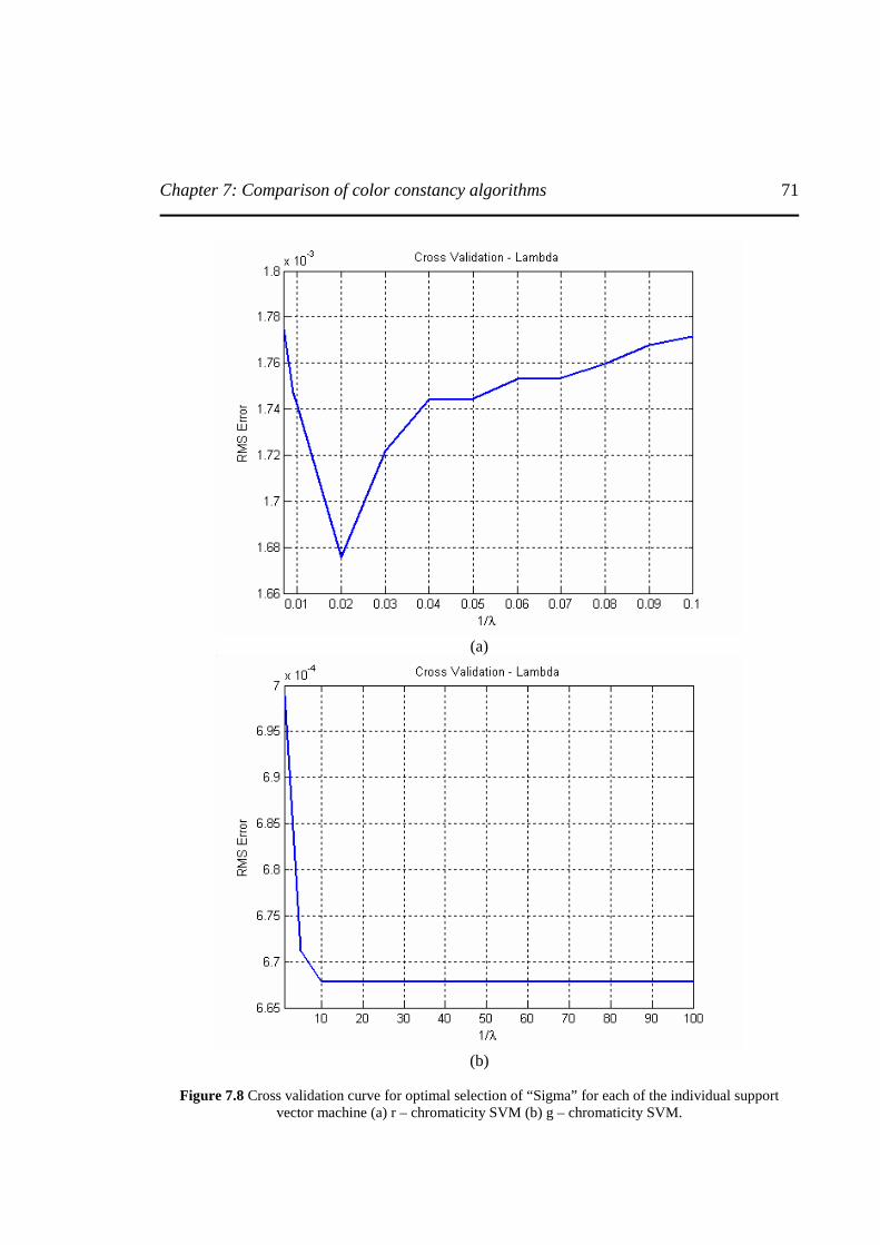
Chapter 7: Comparison of color constancy algorithms
71
(a)
(b)
Figure 7.8 Cross validation curve for optimal selection of “Sigma” for each of the individual support
vector machine (a) r – chromaticity SVM (b) g – chromaticity SVM.
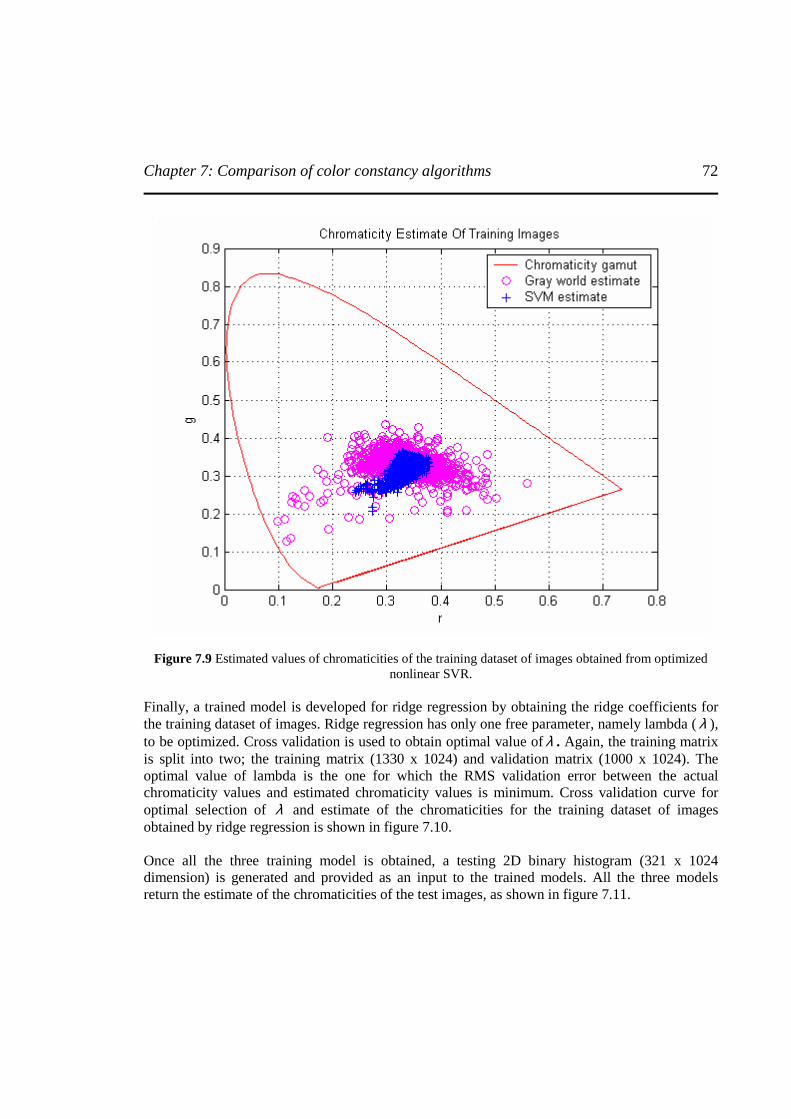
Chapter 7: Comparison of color constancy algorithms
72
Figure 7.9 Estimated values of chromaticities of the training dataset of images obtained from optimized nonlinear SVR.
Finally, a trained model is developed for ridge regression by obtaining the ridge coefficients for the training dataset of images. Ridge regression has only one free parameter, namely lambda (λ ), to be optimized. Cross validation is used to obtain optimal value ofλ . Again, the training matrix is split into two; the training matrix (1330 x 1024) and validation matrix (1000 x 1024). The optimal value of lambda is the one for which the RMS validation error between the actual chromaticity values and estimated chromaticity values is minimum. Cross validation curve for optimal selection of λ and estimate of the chromaticities for the training dataset of images obtained by ridge regression is shown in figure 7.10.
Once all the three training model is obtained, a testing 2D binary histogram (321 x 1024 dimension) is generated and provided as an input to the trained models. All the three models return the estimate of the chromaticities of the test images, as shown in figure 7.11.
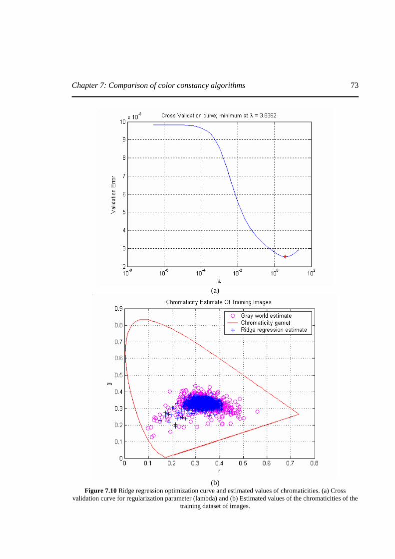
Chapter 7: Comparison of color constancy algorithms
73
(a)
(b)
Figure 7.10 Ridge regression optimization curve and estimated values of chromaticities. (a) Cross validation curve for regularization parameter (lambda) and (b) Estimated values of the chromaticities of the
training dataset of images.
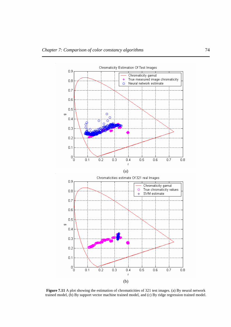
Chapter 7: Comparison of color constancy algorithms
74
(a)
(b)
Figure 7.11 A plot showing the estimation of chromaticities of 321 test images. (a) By neural network trained model, (b) By support vector machine trained model, and (c) By ridge regression trained model.
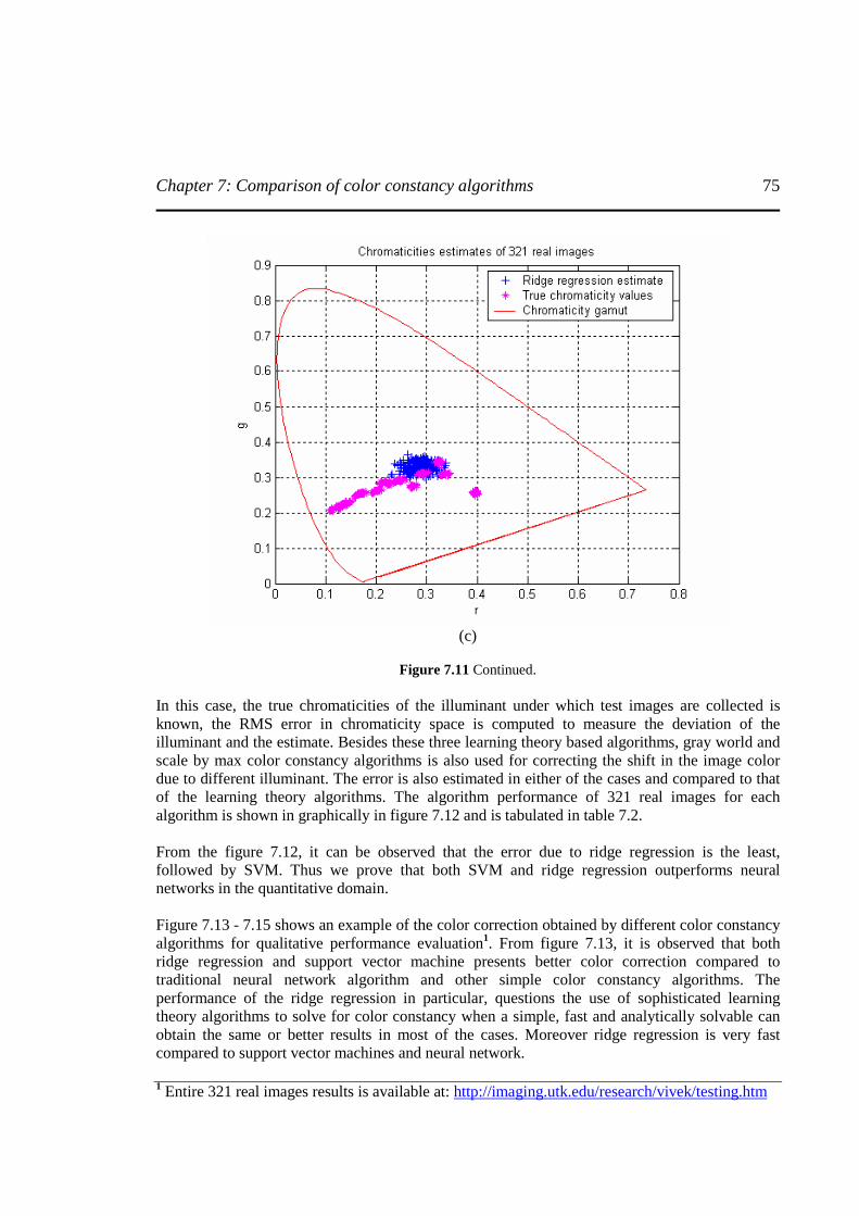
Chapter 7: Comparison of color constancy algorithms
75
(c)
Figure 7.11 Continued.
In this case, the true chromaticities of the illuminant under which test images are collected is known, the RMS error in chromaticity space is computed to measure the deviation of the illuminant and the estimate. Besides these three learning theory based algorithms, gray world and scale by max color constancy algorithms is also used for correcting the shift in the image color due to different illuminant. The error is also estimated in either of the cases and compared to that of the learning theory algorithms. The algorithm performance of 321 real images for each algorithm is shown in graphically in figure 7.12 and is tabulated in table 7.2. From the figure 7.12, it can be observed that the error due to ridge regression is the least, followed by SVM. Thus we prove that both SVM and ridge regression outperforms neural networks in the quantitative domain. Figure 7.13 - 7.15 shows an example of the color correction obtained by different color constancy algorithms for qualitative performance evaluation1. From figure 7.13, it is observed that both ridge regression and support vector machine presents better color correction compared to traditional neural network algorithm and other simple color constancy algorithms. The performance of the ridge regression in particular, questions the use of sophisticated learning theory algorithms to solve for color constancy when a simple, fast and analytically solvable can obtain the same or better results in most of the cases. Moreover ridge regression is very fast compared to support vector machines and neural network.
1 Entire 321 real images results is available at: http://imaging.utk.edu/research/vivek/testing.htm
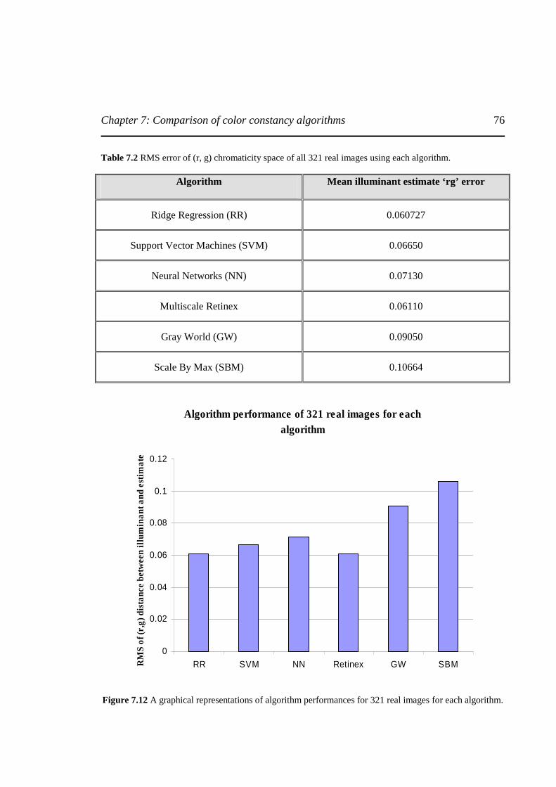
Chapter 7: Comparison of color constancy algorithms
76
Table 7.2 RMS error of (r, g) chromaticity space of all 321 real images using each algorithm.
Algorithm
Mean illuminant estimate ‘rg’ error
Ridge Regression (RR)
0.060727
Support Vector Machines (SVM)
0.06650
Neural Networks (NN)
0.07130
Multiscale Retinex
0.06110
Gray World (GW)
0.09050
Scale By Max (SBM)
0.10664
Algorithm performance of 321 real images for each algorithm
0
0.02
0.04
0.06
0.08
0.1
0.12
RR SVM NN Retinex GW SBMRM
S o
f (r,
g) d
ista
nce
betw
een
illum
ina
nt a
nd e
stim
ate
Figure 7.12 A graphical representations of algorithm performances for 321 real images for each algorithm.
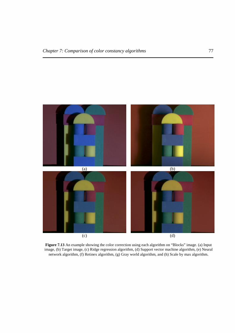
Chapter 7: Comparison of color constancy algorithms
77
(a) (b)
(c) (d)
Figure 7.13 An example showing the color correction using each algorithm on “Blocks” image. (a) Input image, (b) Target image, (c) Ridge regression algorithm, (d) Support vector machine algorithm, (e) Neural
network algorithm, (f) Retinex algorithm, (g) Gray world algorithm, and (h) Scale by max algorithm.
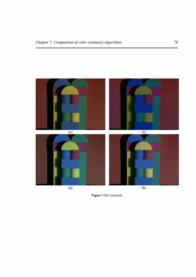
Chapter 7: Comparison of color constancy algorithms
78
(e) (f)
(g) (h)
Figure 7.13 Continued.
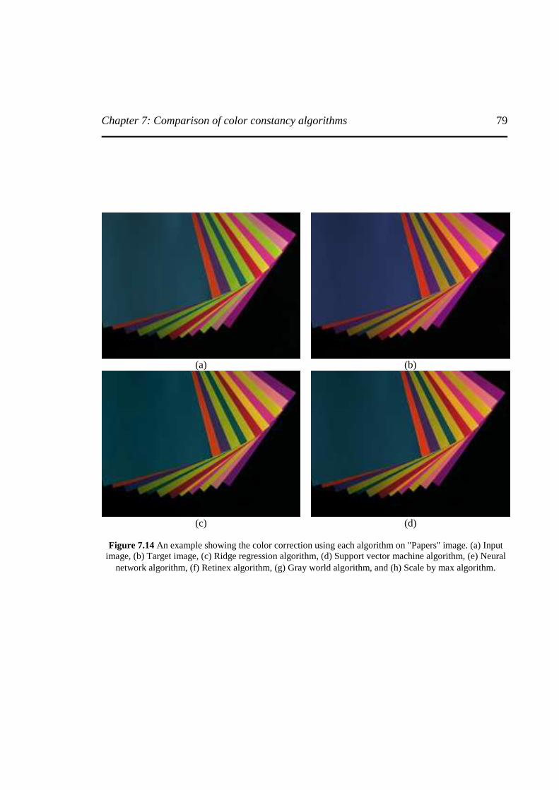
Chapter 7: Comparison of color constancy algorithms
79
(a) (b)
(c) (d)
Figure 7.14 An example showing the color correction using each algorithm on "Papers" image. (a) Input
image, (b) Target image, (c) Ridge regression algorithm, (d) Support vector machine algorithm, (e) Neural network algorithm, (f) Retinex algorithm, (g) Gray world algorithm, and (h) Scale by max algorithm.
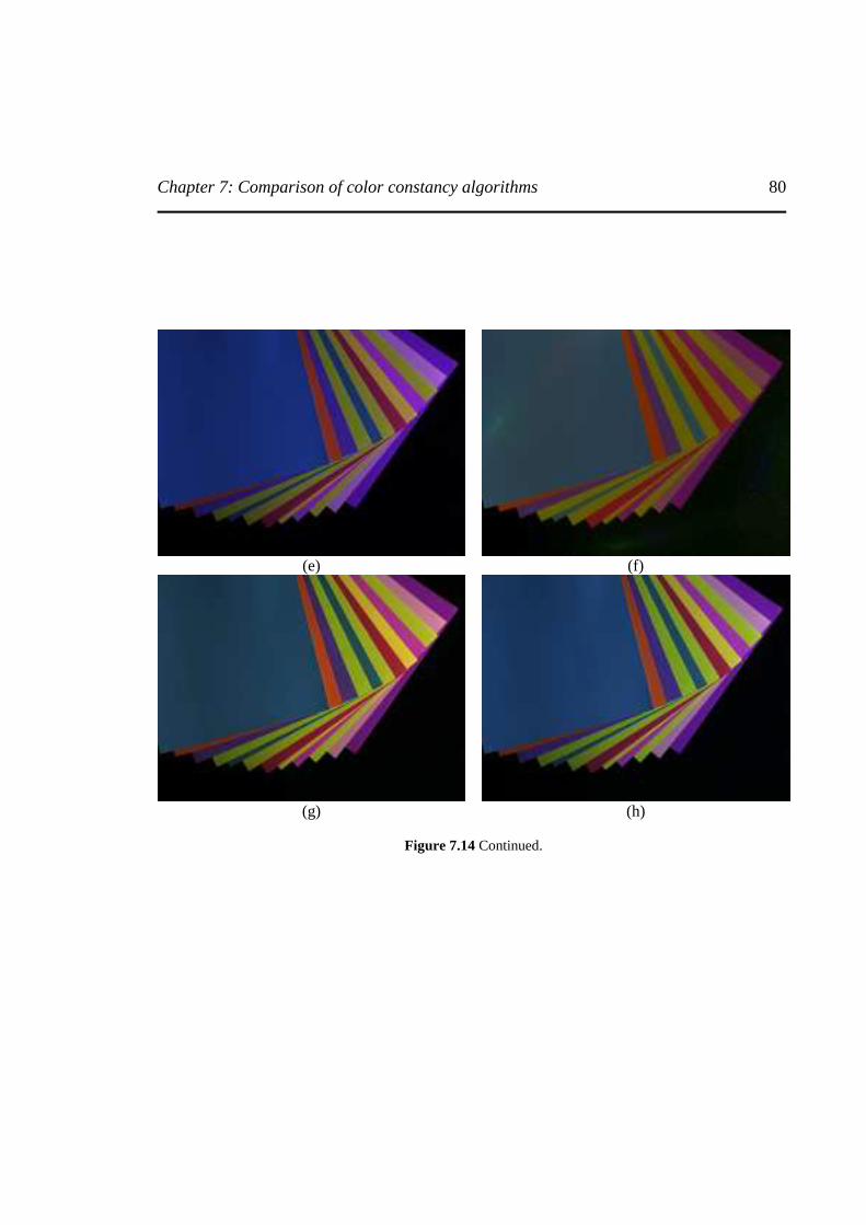
Chapter 7: Comparison of color constancy algorithms
80
(e) (f)
(g) (h)
Figure 7.14 Continued.
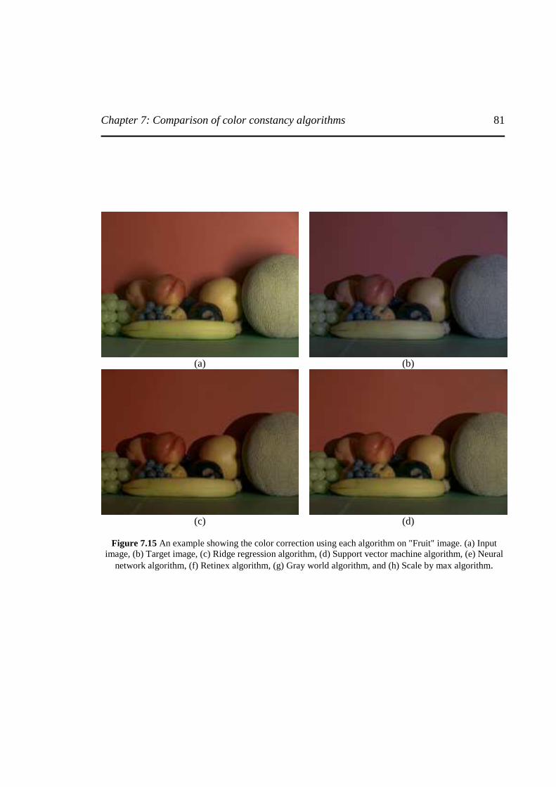
Chapter 7: Comparison of color constancy algorithms
81
(a) (b)
(c) (d)
Figure 7.15 An example showing the color correction using each algorithm on "Fruit" image. (a) Input
image, (b) Target image, (c) Ridge regression algorithm, (d) Support vector machine algorithm, (e) Neural network algorithm, (f) Retinex algorithm, (g) Gray world algorithm, and (h) Scale by max algorithm.
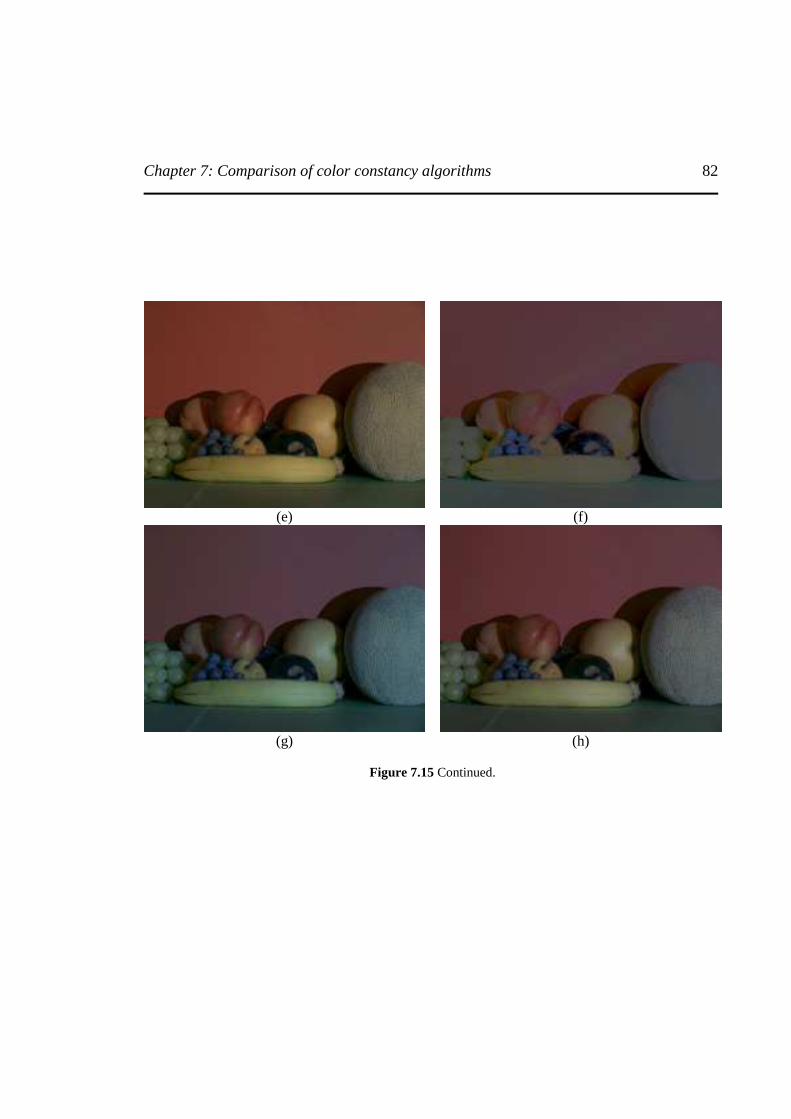
Chapter 7: Comparison of color constancy algorithms
82
(e) (f)
(g) (h)
Figure 7.15 Continued.
Chapter 7: Comparison of color constancy algorithms
83
7.2 Algorithm performance for uncalibrated real images In real time situation, it is very difficult to achieve smooth and homogeneous illumination condition because illumination conditions changes drastically. Unlike controlled environment, practical real time situation presents a unique challenge. Under controlled environment, it is possible to control the illumination variation and measure the actual illuminant value. This helps establish a ground truth. In addition, the affect of noise and highlights can be negated. However, in real time it is practically very difficult to measure the actual value of the illuminant. Moreover affect of atmospheric noise, shadows and highlights are the major area of concern when extending the color constancy algorithms to the real time images. Since in real time situation no ground truth is available, quantitative analysis on the performance of the color constancy algorithm is not possible. Only qualitative performance analysis is possible, which in turn is very subjective. Under this subsection, the performance of each of the color constancy algorithm evaluated for calibrated real images is evaluated for an uncalibrated real time images. A sequence of images of a building in the downtown is collected over a period of day from morning to evening at regular interval of 1 hour to record the variation in the appearance color of the building as the day progresses. Another database of uncalibrated real images of a person walking under inhomogeneous illumination condition is also collected to record the affects of inhomogeneous illumination variation. Both the database of test images are color corrected using the proposed learning theory algorithm and other color constancy algorithms like gray world and scale by max. Both the database of images are presented to the learning theory framework in a similar fashion as calibrated test database of images where presented to the learning theory model as discussed above. Figure 7.16 shows the affect of illumination on the image of a buildings recorded at 3 pm and image recorded at 6 pm. A shuttle difference is clearly visible in the color appearance of the building. Color constancy algorithms are applied to color correct the image and discount the affect of illumination. Figure 7.15 shows the performance of each color constancy algorithm in discounting the affect of illumination. From figure 7.17, it observed that ridge regression continues to provide better color reproduction when compared to neural network and support vector machine algorithms especially. Gray world and scale by max algorithms performs decently well but fails to remove the influence of redness from the input image completely. Similar performance is observed when presented other uncalibrated dataset of image of Ayres Hall also collected over entire day. The performance of each algorithm on Ayres Hall is shown in figure 7.18. In figure 7.19, a sequence of images taken at Knoxville airport under inhomogeneous conditions is corrected using ridge regression. A variation in the appearance of the color of the T-shirt is clearly visible as the person walks through the passage. Since backlight seems to influence the performance of ridge regression only segmented portion of the T-shirt is used to color correct.

Chapter 7: Comparison of color constancy algorithms
84
(a)
(b)
Figure 7.16 An image of a downtown taken at different time of a day showing the effect of
llumination variation on the color appearance of the building. (a) Image captured at 3 pm and (b) Image captured at 6 pm.
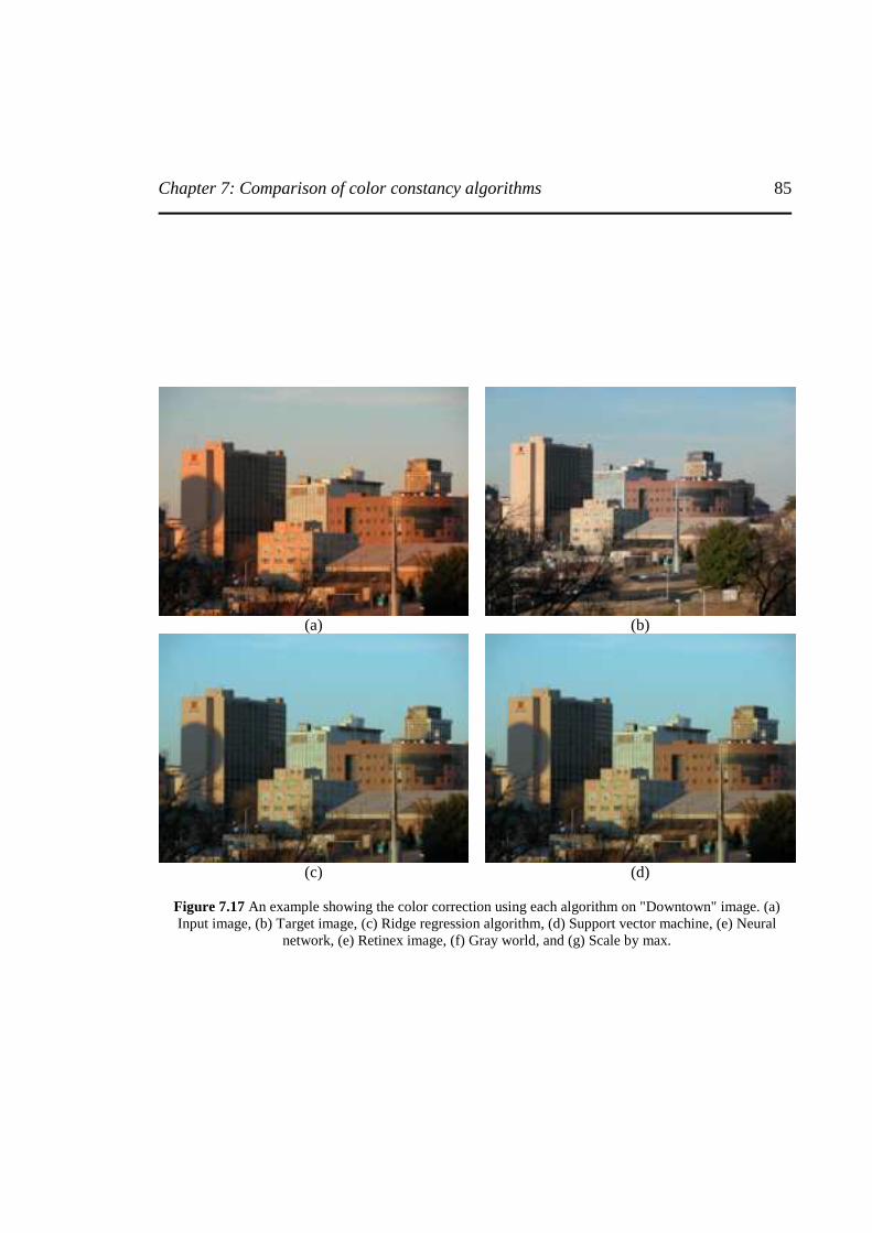
Chapter 7: Comparison of color constancy algorithms
85
(a) (b)
(c) (d)
Figure 7.17 An example showing the color correction using each algorithm on "Downtown" image. (a) Input image, (b) Target image, (c) Ridge regression algorithm, (d) Support vector machine, (e) Neural
network, (e) Retinex image, (f) Gray world, and (g) Scale by max.
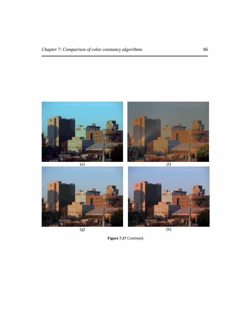
Chapter 7: Comparison of color constancy algorithms
86
(e) (f)
(g) (h)
Figure 7.17 Continued.
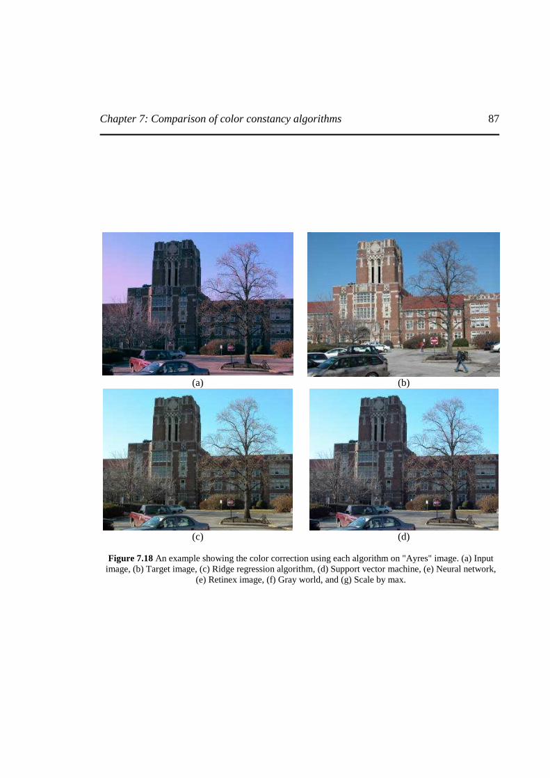
Chapter 7: Comparison of color constancy algorithms
87
(a) (b)
(c) (d)
Figure 7.18 An example showing the color correction using each algorithm on "Ayres" image. (a) Input image, (b) Target image, (c) Ridge regression algorithm, (d) Support vector machine, (e) Neural network,
(e) Retinex image, (f) Gray world, and (g) Scale by max.
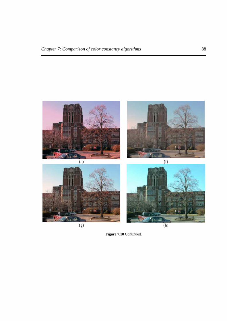
Chapter 7: Comparison of color constancy algorithms
88
(e) (f)
(g) (h)
Figure 7.18 Continued.
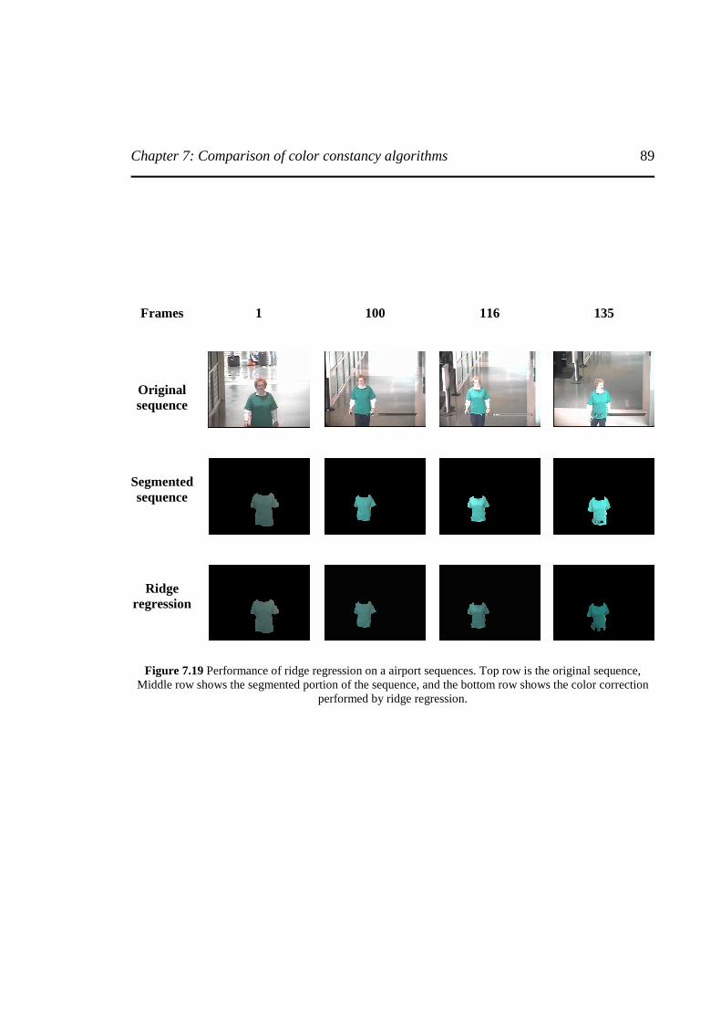
Chapter 7: Comparison of color constancy algorithms
89
Frames
1
100
116
135
Original sequence
Segmented sequence
Ridge regression
Figure 7.19 Performance of ridge regression on a airport sequences. Top row is the original sequence, Middle row shows the segmented portion of the sequence, and the bottom row shows the color correction
performed by ridge regression.
Chapter 7: Comparison of color constancy algorithms
90
7.3 Analysis of Algorithm performances In this thesis, five color constancy algorithms performance on color correcting both the calibrated and uncalibrated real images is shown. Out of the five methods, gray world and scale by max algorithms are the simple color balancing algorithms, which color corrects the images by scaling each channel individually with a scale factor. The scale factor is computed by computing the mean value and the maximum value in each channel for gray world and scale by max algorithm respectively. But the simplicity of both the algorithms is negated by the unreliable color correction it produces when presented with different color varied images. Remaining three algorithms; neural network approach, support vector approach and ridge regression approach are the learning theory approaches. They are also referred as ‘Machine learning’. In the case of learning theory based approaches, the color correction is performed utilizing the knowledge of a trained model developed during the training phase. The trained model is adaptive in nature and learns the dependency between the illuminant and surface reflectance from the training set of images. Generating a trained model becomes little easy if the range of variation of the illuminant chromaticity is known. In our case, the range of chromaticity variation is approximately known. Gray world algorithm assumes the average surface reflectance of a typical scene is ‘gray’ and any deviation from that value corresponds to shift in color of the image. However, this does not hold good for most of the real images collected either in controlled conditions or in drastically varying illumination conditions. The performance of gray world algorithm is better on the images collected under controlled and smoothly varying illumination conditions when compared to the situation of sudden changing and inhomogeneous illumination conditions. Scale by max on a similar note to gray world suffers for some disadvantages which negates its simplicity of approach. Scale by max is considered to be simple form of statistical algorithm [Brainard’97] and also limiting aspect of one of many versions of Retinex [Horn’74]. This method is sensitive to the dynamic range of the vision system. In the world of matte reflectance, the estimate of the illuminant magnitude will be biased; therefore the maximum reflectance value will always be less than 255. This accounts for inaccurate estimate. Additionally, the presence of specularities may result in reflectance values greater than 255, which again will lead to incorrect estimation. Neural network approach to color constancy introduced the application of learning theory to solve for color constancy. This approach showed the utilization of multilayer preceptron comprising of different neuron architecture can be used to develop a trained model from the training set of images by readjusting the weights of the neurons. However, neural network approach to color constancy is an ill-posed approach to solve an ill-posed problem. There are number of issues in the approach that leads to serious discussion on the creditability of the results obtained by the neural network. The results obtained using neural network cannot be guaranteed. The neural network approach has many parameters to control like initialization of weights, learning rate, training goal, network architecture and training approach. It is very difficult to regularize all the parameters of the neural networks. The ill-posedness of the neural network approach is shown by changing the network architecture and affect of initialization of weights on the training process.
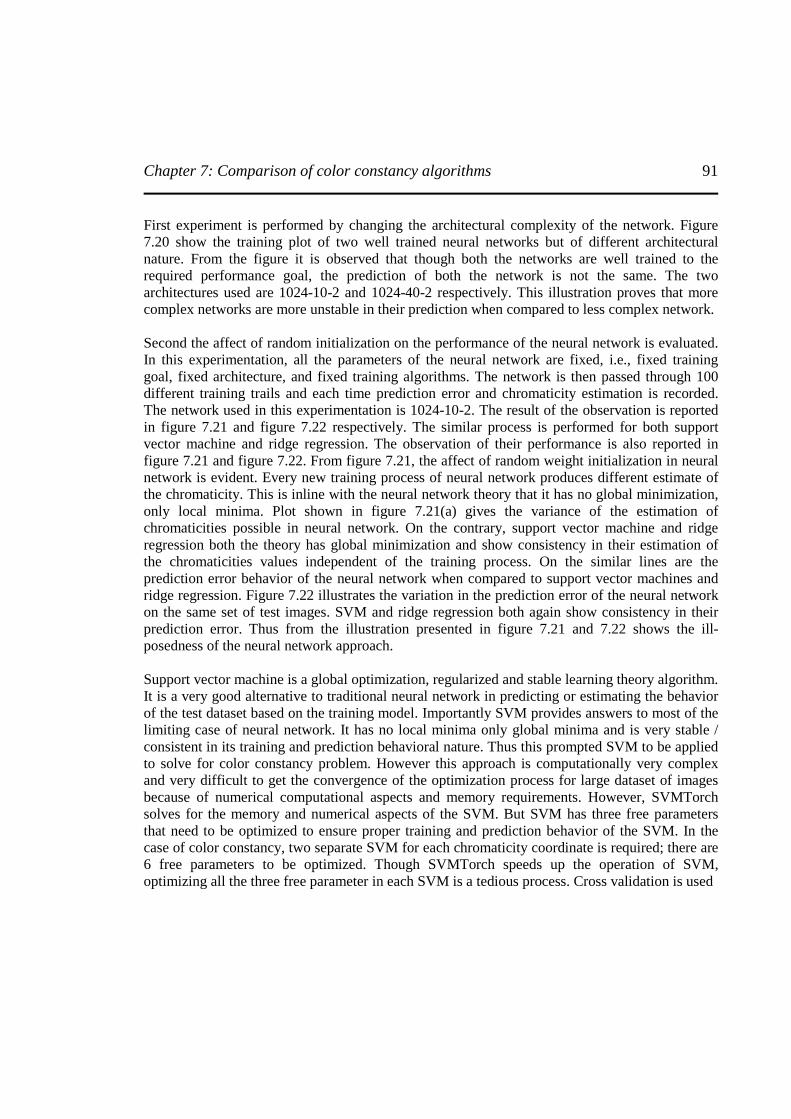
Chapter 7: Comparison of color constancy algorithms
91
First experiment is performed by changing the architectural complexity of the network. Figure 7.20 show the training plot of two well trained neural networks but of different architectural nature. From the figure it is observed that though both the networks are well trained to the required performance goal, the prediction of both the network is not the same. The two architectures used are 1024-10-2 and 1024-40-2 respectively. This illustration proves that more complex networks are more unstable in their prediction when compared to less complex network. Second the affect of random initialization on the performance of the neural network is evaluated. In this experimentation, all the parameters of the neural network are fixed, i.e., fixed training goal, fixed architecture, and fixed training algorithms. The network is then passed through 100 different training trails and each time prediction error and chromaticity estimation is recorded. The network used in this experimentation is 1024-10-2. The result of the observation is reported in figure 7.21 and figure 7.22 respectively. The similar process is performed for both support vector machine and ridge regression. The observation of their performance is also reported in figure 7.21 and figure 7.22. From figure 7.21, the affect of random weight initialization in neural network is evident. Every new training process of neural network produces different estimate of the chromaticity. This is inline with the neural network theory that it has no global minimization, only local minima. Plot shown in figure 7.21(a) gives the variance of the estimation of chromaticities possible in neural network. On the contrary, support vector machine and ridge regression both the theory has global minimization and show consistency in their estimation of the chromaticities values independent of the training process. On the similar lines are the prediction error behavior of the neural network when compared to support vector machines and ridge regression. Figure 7.22 illustrates the variation in the prediction error of the neural network on the same set of test images. SVM and ridge regression both again show consistency in their prediction error. Thus from the illustration presented in figure 7.21 and 7.22 shows the ill-posedness of the neural network approach. Support vector machine is a global optimization, regularized and stable learning theory algorithm. It is a very good alternative to traditional neural network in predicting or estimating the behavior of the test dataset based on the training model. Importantly SVM provides answers to most of the limiting case of neural network. It has no local minima only global minima and is very stable / consistent in its training and prediction behavioral nature. Thus this prompted SVM to be applied to solve for color constancy problem. However this approach is computationally very complex and very difficult to get the convergence of the optimization process for large dataset of images because of numerical computational aspects and memory requirements. However, SVMTorch solves for the memory and numerical aspects of the SVM. But SVM has three free parameters that need to be optimized to ensure proper training and prediction behavior of the SVM. In the case of color constancy, two separate SVM for each chromaticity coordinate is required; there are 6 free parameters to be optimized. Though SVMTorch speeds up the operation of SVM, optimizing all the three free parameter in each SVM is a tedious process. Cross validation is used
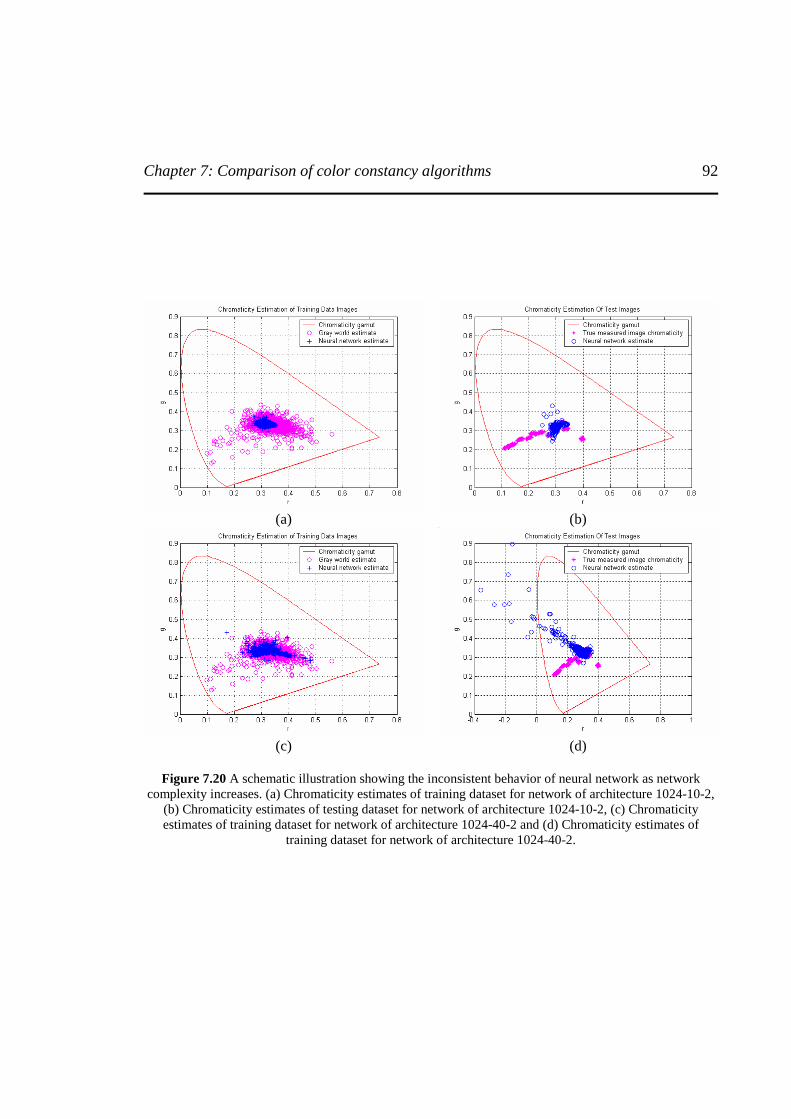
Chapter 7: Comparison of color constancy algorithms
92
(a) (b)
(c) (d)
Figure 7.20 A schematic illustration showing the inconsistent behavior of neural network as network
complexity increases. (a) Chromaticity estimates of training dataset for network of architecture 1024-10-2, (b) Chromaticity estimates of testing dataset for network of architecture 1024-10-2, (c) Chromaticity estimates of training dataset for network of architecture 1024-40-2 and (d) Chromaticity estimates of
training dataset for network of architecture 1024-40-2.
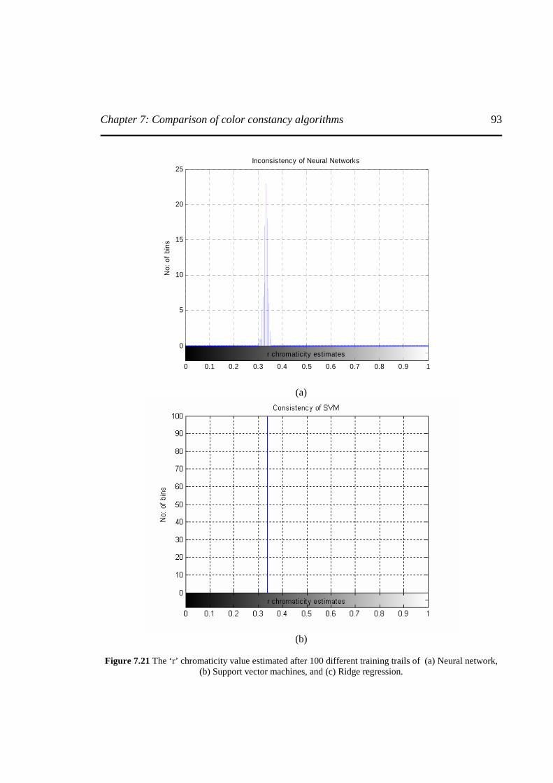
Chapter 7: Comparison of color constancy algorithms
93
0 0.1 0.2 0.3 0.4 0.5 0.6 0.7 0.8 0.9 1
0
5
10
15
20
25
r chromaticity estimates
No:
of
bins
Inconsistency of Neural Networks
(a)
(b)
Figure 7.21 The ‘r’ chromaticity value estimated after 100 different training trails of (a) Neural network,
(b) Support vector machines, and (c) Ridge regression.
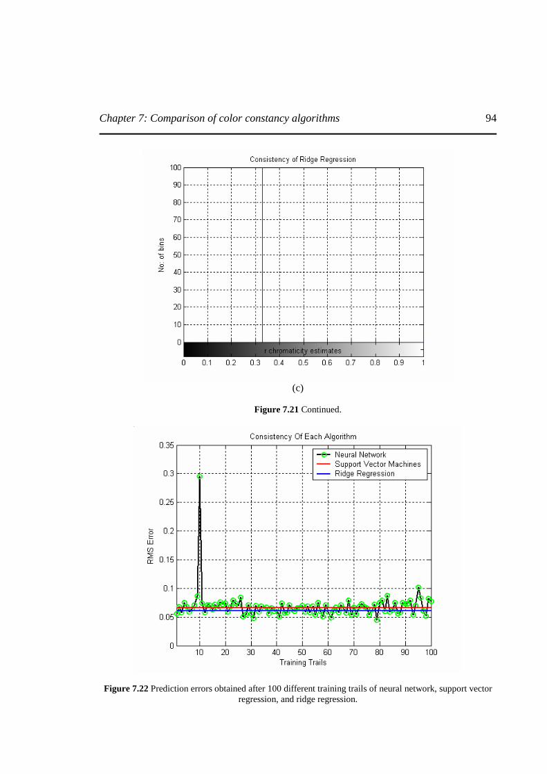
Chapter 7: Comparison of color constancy algorithms
94
(c)
Figure 7.21 Continued.
Figure 7.22 Prediction errors obtained after 100 different training trails of neural network, support vector regression, and ridge regression.

Chapter 7: Comparison of color constancy algorithms
95
to optimize the parameters. Since cross validation prone to fail, it is even difficult to optimize the parameters correctly. Ridge regression is also a learning theory based approach. The best part of this approach is that it is simple, fast and analytically solvable unlike its counterpart neural network and support vector machines. From quantitative and qualitative algorithm evaluation on both calibrated real images and uncalibrated real images, it is observed that the performance of ridge regression is same or better than neural network and SVM. The merits of this approach lay down a question on the use of complex and sophisticated learning theory algorithms. Unlike neural network it has global minima and is very stable / consistent in its behavior. In comparison to support vector machines, both the methods have global minima and are stable / consistent their behavior but ridge regression has on one free parameter to optimize. Cross validation is used to optimize the free parameter. Optimal selection of free parameter (Lambda) is very important because if a large value of lambda is selected the ridge regression coefficient decreases and prediction starts to shrink. Thus it is also known as shrinkage algorithm. Thus this chapter presented a thorough discussion on the results and analysis of algorithm performance in detail discussing the advantages and disadvantages of each of the algorithm.

Chapter 8: Conclusion and future work
96
Chapter 8
8 CONCLUSION AND FUTURE WORK This final chapter pens down the concluding remarks on the work performed and presented in this thesis document on ‘Machine learning approach to color constancy’. The contribution of this work will help numerous computer vision applications. Any research work presents endless scope to improve and grow in future, so does this research work. Finally, we discuss the possible scope and improvement of the current research as a next step that would possible benefit to future research in this field. The subsection 8.1 presents the conclusion on the present research work and future aspects of this research are discussed in subsection 8.2.
8.1 Conclusions The major objective of any color constancy algorithm is to discount the affect of illumination on the color image formation. In other words negates the shift in the chromaticity of the images due to chromaticity of the different illuminants. The classification of color constancy algorithms apprised the reader with different aspects of the color constancy algorithms. Our motivation behind this research was motivated towards obtaining an approach that presents stable color reproduction and is computationally less complex. The contribution of this research work is two machine learning theory based color constancy algorithms namely ‘Support vector regression’ and ‘Ridge regression’. Both the contribution achieves stable and consistent color reproduction in comparison to methods discussed in literature but former is computationally complex compared to later. In the context of the motivation and results, the ridge regression is the more fitting contribution of this work. It is simple, fast, reliable and stable approach. All the algorithms in the literature make some assumption about the statistics of the reflectance to be encountered, and most make assumptions about the illuminants that will be encountered. The gray world algorithm makes assumption about the expected value of scene average, scale by max algorithm makes the assumption about the maximum value in each channel and the gamut mapping algorithms makes the assumptions about the ranges of expected reflectances and illuminants. Besides these specific assumptions each of the algorithms makes additional assumption of flat surface, homogeneous illumination conditions. Color by correlation and neural network however does not make any prior assumption on surface reflectance and illuminant. As assumptions goes stronger, greater the vulnerability of the algorithm as the assumption fails. It is shown by [Barnard’02b], currently the best performance is obtained by gamut mapping, a constraint based approach. But at the same time [Funt’98] also shows, even gamut mapping is not
Chapter 8: Conclusion and future work
97
good enough for object recognition. Therefore there is search of algorithm that can take reasonable assumptions in to account and perform well. Our research explored the possibilities of applying machine learning approach to solve for color constancy for reasons that; Machine learning theories based algorithms do not make any specific assumption on the surface reflectance and illumination, but rather goes ahead and models the distribution. They are distribution free approaches. Neural network, support vector machine and ridge regression exploit only reasonable assumptions, preferably backed by empirical studies. All the approaches are adaptive. Our experimentation showed that learning theory based algorithms are better at estimating the chromaticities of the illuminant in case of both calibrated and uncalibrated real images dataset when no information is available compared to other approaches. The adaptive nature of the algorithms enables them to adapt to the changing conditions more smartly. In our experiments, we took care to avoid the presence of specularities. The occurrence of specularities affected the performance of learning theory algorithms to methods like gamut mapping. Looking inside the machine learning theory approaches, detailed analysis of all the three approaches; neural network, support vector machines and ridge regression proved that neural network is an ill-posed approach compared to other two machine learning theory approaches. Our experimentation proved that a neural network is an unstable, unreliable approach. The results obtained by neural network cannot be guaranteed and very difficult to regularize. Experimental studies also showed that support vector machine and ridge regression behave in a similar fashion; in terms of training and prediction processes. But the complexity of the SVM stands as its major drawback and proves as a major advantage for ridge regression. Presenting an argument against not using color by correlation, though it also models the distribution is because it is shown by [Cardei’02] that color by correlation on average is outperformed by neural network.
8.2 Future work The work in this thesis presents scope for future research in evaluating the number of aspects of machine learning approaches to solve for color constancy. This research has two parts. Machine learning theories and color constancy. Each of the part has their own issues to be addressed in order to improve and get good color constancy. As shown in machine learning theory approach it is very important to select the free parameters appropriately. Improper selection of the parameters will lead to incorrect chromaticity training model and affecting the prediction accuracy. In our case, we use cross validation to select the parameters based on the validation error. Cross validation is a good technique but not the most reliable one. It is prone to failure. It not always presents global unique minimization of the error. Local minima values do occur in cross validation and even global unique solution does not guarantee to be a best of the criteria for parameter selection. For now this is an affective technique but in future to seek robustness in the use of machine theories to solve for color constancy investigation into robust parameter selection is important.
Chapter 8: Conclusion and future work
98
In case of color constancy approach, the present approach shows limitation to the presence of highlights and backlights. Possible reason behind this is because of lack of training images with highlights and backlights. At present, we develop a training model within a limited range of chromaticity values. Expanding the range of chromaticities of illuminant occurring in nature will help to developing better training model to cope with highlights and backlights. Another issue is sampling of chromaticity space. We convert the training and testing datasets into 2D binary histogram by sampling the chromaticity space. Sampling describes the number of bins of chromaticity values used to develop the training model. Small number of bins presents less accurate estimate to develop the training model and large number of bins increases the time to build a training model. This trade off is of little importance in case of ridge regression but this trade off affects the prediction accuracy of the chromaticities in the test images. Heuristic approach is adopted at present. A sound method to balance this trade off is area of future research. After presenting thorough analysis of our contribution on machine learning approach to color constancy and its future prospects, we pen off with the hope that with this effort we moved a step closer in direction of achieving human color constancy in computer vision.

99
REFERENCES
References
100
REFERENCES [Barnard’02] K. Barnard, and B. Funt, “Camera characterization for color research,” Color Research and Application, vol. 27, no. 3, pp. 153-164, 2002. [Barnard’02a] K. Barnard, V. C. Cardei, and B. V. Funt, “A comparison of computational color constancy algorithms-Part I: Methodology and Experiments with Synthesized data,” IEEE Transaction on Image Processing, vol. 11, no. 9, pp. 972-983, 2002. [Barnard’02b] K. Barnard, L. Martin, A. Coath, and B. V. Funt, “A comparison of computational color constancy algorithms-Part II: Experiments with Image data,” IEEE Transaction on Image Processing, vol. 11, no. 9, pp. 985-996, 2002. [Barnard’02c] K. Barnard, L. Martin, B. Funt, and A. Coath, “A data set for color research,” Color Research and Application, vol. 27, no. 3, pp.147-151, 2002. http://www.cs.sfu.ca/~colour/data/colour_constancy_test_images/ [Barnard’01] K. Barnard, F. Ciurea, and B. Funt, “Spectral sharpening for computational color constancy,” Journal of Optical Society of America A, vol. 18, pp. 2728-2743, 2001. [Barnard’00a] K. Barnard, L. Martin, and B. Funt, “Color by correlation in a three dimensional color space,” Proceeding of 6th European Conference on Computer Vision, pp. 375-389, 2000. [Barnard’00b] K. Barnard, “Improvements to gamut mapping color constancy algorithms,” Proceedings in 6th European Conference on Computer Vision, pp. 390-402, 2000. [Barnard’99] K. Barnard, “Practical color constancy,” Ph.D. Dissertation, Simon Fraser University, School of Computer Science, BC, Canada, 1999. [Barnard’98] K. Barnard, and B. V. Funt, “Investigations into Multiscale Retinex,” Color Imaging in Multimedia, pp. 9-17, 1998. [Barnard’97] K. Barnard, G. Finlayson, and B. Funt, “Color constancy for scenes with varying illumination,” Computer Vision Image Understanding, vol. 65, pp. 311-321, 1997. [Barnard’95] K. Barnard, “Computational Color Constancy: Taking Theory into Practice,” M.Sc thesis, Simon Fraser Univ., School of Computing Science, BC, Canada, 1995. [Brainard’97b] D. H. Brainard, and W. T. Freeman, “Bayesian color constancy,” Journal of Optical Society of America A, vol. 14, pp. 1393-1411, 1997. [Bishop’96] C. M. Bishop, “Neural network for Pattern Recognition,” Oxford University Press, Oxford, 1996.
References
101
[Blake’85] A. Blake, “Boundary conditions for lightness computation in Mondrian world,” Computer Vision, Graphics and Image Processing, vol. 32, pp.314-327, 1985. [Buchsbaum’80] G. Buchsbaum, “A Spatial processor model for object color perception,” Journal of Franklin Institute, vol. 310, pp. 1-26, 1980. [Cardei’02] V. Cardei, B. V. Funt, and K. Barnard, “Estimating the Scene Illumination Chromaticity Using a Neural Network,” Journal of the Optical Society of America A, vol. 19, no. 12, pp. 2374 – 2386, Dec 2002. [Cardei’99a] V. Cardei, B. V. Funt, and K. Barnard, “White point estimation for uncalibrated images,” Proceedings of the IS&T/SID, 7th Color Imaging Conference: Color Science, Systems and Applications, pp. 97-100, 1999. [Cardei’99b] V. Cardei, and B. V. Funt, “Committee based Color constancy,” Proceedings of the IS&T/SID, 7th Color Imaging Conference: Color Science, Systems and Applications, pp 311-313, 1999. [Cardei’97] V. Cardei, B. V. Funt, and K. Barnard, “Modeling color constancy with Neural Networks,” in Proceeding of International Conference on Vision, Recognition, and Action: Neural Models of Mind and Machine, May 29-31, 1997. [Chapron’92] M. Chapron, “A new chromatic edge detector used for color image segmentation,” IEEE International Conference on Pattern Recognition, A, pp. 311-314, 1992. [Chernick’99] M. R. Chernick, “Bootstrapping Methods: A Practitioner’s Guide,” Wiley series in probability and statistics, John Wiley & Sons Ltd, NY, USA, 1999. [Collobert’01] R. Collobert, and S. Bengio, “Support Vector Machines for Large-Scale Regression Problems,” Journal of Machine Learning Research, vol. 1, pp. 143-160, 2001. [Cooper’04] T. J. Cooper, and F. A, Baqai, “Analysis and extensions of the Frankle-McCann Retinex algorithm,” Journal of Electronic Imaging, vol. 13, no. 1, pp. 85-92, 2004. [Ciurea’04] F. Ciurea, and B. V. Funt, “Tuning Retinex parameters,” Journal of Electronic Imaging, vol. 13, no. 1, pp. 58-64, 2004. [D’Zmura’94] M. D’Zmura, and G. Iverson, “Probabilistic Color Constancy,” Geometric Representations of Perceptual Phenomena: Papers in honor of Tarow Indow’s 70th Birthday. Laurence Erlbaum Associates, 1994. [D’Zmura’93] M. D’Zmura, and G. Iverson, “Color constancy. I. Basic theory of two stage linear recovery of spectral descriptions for lights and surfaces,” Journal of Optical Society of America A, vol. 10, pp. 2148-2156, 1993.

References
102
[Denison’02] D. G. T. Denison, C. C. Holmes, B. K. Mallick, and A. F. M. Smith, “Bayesian Methods for Nonlinear classification and regression,” Wiley series in probability and statistics, John Wiley & Sons Ltd, NY, USA, 2002. [Darper’98] N. R. Draper, and H. Smith, “Applied Regression Analysis-Third Edition,” Wiley Series in Probability and Statistics, John Wiley & Sons, Inc. 1998. [Ebner’04] M. Ebner, “A parallel algorithm for color constancy,” Journal of Parallel and Distributed Computing, vol. 64, no. 1, pp. 79-88, 2004. [Fairchild’97] M. D. Fairchild, “Color appearance models,” Addison Wesley Longman, Inc, 1997. [Farid’01] H. Farid, “Blind inverse gamma correction,” IEEE Transaction on Image Processing, vol. 10, no. 10, pp. 1428 – 1433, 2001. [Flake’00] G. Flake, and S. Lawrence, “Efficient SVM regression training with SMO,” Journal of Machine learning, 2001. [Finlayson’01] G. H. Finlayson, S. D. Hordley, and P. M. Hubel, “Color by correlation: A simple, unifying framework for color constancy,” IEEE Transaction on Pattern Analysis and Machine Intelligence, vol. 23, no. 11, pp. 1209-1221, 2001. [Finlayson’00] G. H. Finlayson, and S. Hordley, “Improving Gamut Mapping Color constancy,” IEEE Transaction on Image Processing, vol. 9, no. 10, pp. 1774-1783, 2000. [Finlayson’99] G. H. Finlayson and S. D. Hordley, “Selection for gamut mapping color constancy", Image and Vision Computing, vol. 17, no. 8, pp. 597-604, 1999. [Finlayson’98] G. H. Finlayson and S. D. Hordley, “A theory of selection for gamut mapping color constancy,” IEEE conference on Computer Vision and Pattern Recognition, Santa Barbara, pp. 60-65, 1998. [Finalyson’97] G. D. Finlayson, P. H. Hubel, and S. Hordley, “Color by correlation,” in Proceeding of IS&T?SID, 5th Color Imaging Conference: Color Science, Systems and Applications, Scottsdale, AZ, pp. 6 -11, 1997. [Finlayson’96] G. H. Finlayson, “Color in perspective,” IEEE Transaction on Pattern Analysis and Machine Intelligence, vol. 18, no. 10, pp. 1034-1038, 1996. [Finlayson’95a] G. H. Finlayson, “Color constancy in diagonal chromaticity space,” IEEE Proceeding of 5th International Conference on Computer Vision, pp. 218-223, 1995. [Finlayson’95b] G. H. Finlayson, “Coefficient color constancy,” Ph.D. Dissertation, Simon Fraser University, School of Computer Science, BC, Canada, 1995.
References
103
[Finlayson’94a] G. H. Finlayson, M. S. Drew, and B. V. Funt, “Spectral sharpening: Sensor transformations for improved color constancy,” Journal of Optical Society of America A, vol. 11, pp. 1553-1563, 1994. [Finlayson’94b] G. H. Finlayson, M. Drew, and B. H. Funt, “Color constancy: Generalized Diagonal Transforms Suffice,” Journal of Optical Society of America A, vol. 11, no. 11, pp. 3011-3020, 1994. [Finlayson’93] G. H. Finlayson, M. Drew, and B. V. Funt, “Diagonal transforms suffice for color constancy,” IEEE International Conference on Computer Vision, pp. 163-171, 1993. [Freeman’95] W. T. Freeman, and D. H. Brainard, “Bayesian Decision Theory, the Maximum Local Mass Estimate, and Color Constancy,” IEEE 5th International Conference on Computer Vision, 1995. [Forsyth’90] G. D. Forsyth, “A Novel algorithm for color constancy,” International Journal of Computer Vision, vol. 5, no.1, pp. 5-36, 1990. [Funt’04] B. V. Funt, F. Ciurea, and J. McCann, “Retinex in MATLAB,” Journal of Electronic Imaging, vol. 13, no. 1, pp. 48-57, 2004. [Funt’01] B. V. Funt, and F. Ciurea, “Parameters for Retinex,” AIC Proceedings of 9th Congress of the International Color Association, Rochester, June 2001. [Funt’99a] B. V. Funt, V. C. Cardei, and K. Barnard, “Method of estimating chromaticity of illumination using neural networks,” U.S. Patent 5 907 629, 1999. [Funt’99b] B. V. Funt and V. Cardei, “Bootstrapping Color constancy,” in Proceedings of SPIE, Electronic Imaging IV, vol. 3644, 1999. [Funt’98] B.V. Funt, K. Barnard, and L. Martin, “Is color constancy good enough?” in Proceedings of 5th European Conference on Computer Vision, pp. 445-459, 1998. [Funt’97a] B. V. Funt, V. C. Cardei, and K. Barnard, “Learning color constancy.” Proceedings of IS&T/SID 5th Color Imaging Conference: Color Science Systems, and Applications, pp. 6-11, 1997. [Funt’97b] B. V. Funt, K. Barnard, K. Brockington, and V. C. Cardei, “Luminance based multiscale Retinex,” AIC International Color Association, 1997. [Funt’95] B. V. Funt, and G. H. Finlayson “Color constancy color indexing,” IEEE Transaction on Pattern Analysis and Machine Intelligence, vol.17, no.5, pp.552 – 529, 1995. [Funt’93] B. V. Funt and M. S. Drew, “Color space analysis of mutual illumination,” IEEE Transaction on Pattern Analysis and Machine Intelligence, vol. 15, no. 12, pp. 1319-1326, 1993.
References
104
[Funt’92] B. V. Funt, M. S. Drew, and M. Brockington, “Recovering shading from color images,” Proceedings of 2nd European Conference on Computer Vision, pp. 124-132, 1992. [Funt’91] B. V. Funt, M. S. Drew, and J. Ho, “Color constancy from mutual reflection,” International Journal of Computer Vision, vol. 6, pp. 5-24, 1991. [Gonzalez’01] R. C. Gonzalez, and R. E. Woods, “Digital Image Processing.” Second Edition, Prentice Hall Inc, 2001. [Gershon’88] R. Gershon, A. D. Jepson, and J. K. Tsotsos, “From [r,g,b] to surface reflectance: Computing color constant descriptors in images perception,” pp.755-758, 1988. [Horn’74] B. K. P. Horn, “Determining lightness from an image,” Computer Vision, Graphics and Image Processing, vol. 3, pp. 277-299, 1974. [Hurlbert’89] A. C. Hurlbert, “The Computation of Color,” PhD Dissertation, Massachusetts Institute of Technology, September, 1989. [Jobson’97] D. J. Jobson, Z. Rahman, and G. A. Woodell, “Properties and Performance of a Center/Surround Retinex,” IEEE Transactions on Image Processing, vol. 6, no. 3, pp. 451-462, 1997. [Joachims’99] T. Joachims, “Making large-Scale SVM Learning Practical,” Advances in Kernel Methods - Support Vector Learning, B. Schölkopf and C. Burges and A. Smola (ed.), MIT Press, 1999. [Kecman’01] V. Kecman, “Learning and Soft Computing: Support vector machine, neural networks and fuzzy logic models,” MIT Press, Cambridge, London, 2001. [Kimmel’03] R. Kimmel, M. Elad, D. Shaked, R. Keshet, and I. Sobel, “A Variational framework for Retinex,” International Journal of Computer Vision, vol. 52, no.1, pp. 7-23,2003. [Land’77] E. H. Land, “The Retinex theory of color constancy,” Scientific America, pp. 108-129, 1977. [Lee’86] H. C. Lee, “Method for computing the scene-illuminant chromaticity from specular highlights,” Journal of Optical Society of America A, vol. 3, pp. 1964-1969, 1986. [Lin’00] C. Lin, “On the Convergence of the Decomposition Methods for Support Vector Machines,” National Taiwan University. [Lippmann’87] R. P. Lippmann, “An introduction to computing with Neural Nets,” IEEE ASSP Magazine (also IEEE Signal Processing Magazine), vol. 4, no. 2, pp. 4-22, 1987. [Maloney’86a] L. T. Maloney, and B. A. Wandell, “Color Constancy: A method for recovering surface reflectance,” Journal of Optical Society of America A, vol. 3, no. 1, pp. 29-33, 1986.
References
105
[Maloney’86b] L. T. Maloney, “Evaluation of linear models of surface spectral reflectance with small number of parameters,” Journal of Optical Society of America A, vol. 3 no. 10, pp.1673-1683, 1986. [Maloney’85] L.T. Maloney, “Computational Approach to Color constancy,” Stanford University Applied Psychology Laboratory, 1985. [Mattera’99] D. Mattera, and S. Haykin, “Support Vector Machines for Dynamic Reconstruction of a Chaotic System,” In B. Scholkopf, C. Burges, and A. Smola (Eds.), Advances in Kernel Methods. The MIT Press, 1999. [Moore’91] A. Moore, J. Allman, and R. M. Goodman, “A real time neural system for color constancy,” IEEE Transaction on Neural Network, vol. 2, no. 2, pp. 237-247, 1991. [Nimeroff’72] I. Nimeroff, “Colorimetry. In Precision Measurement and Calibration,” Selected NBS Papers on Colorimetry, vol. 9, pp. 157-203, 1972. [Orchard’91] M. T. Orchard, and C. A. Bouman, “Color quantization of images,” IEEE Transaction on Signal Processing. Vol. 39, no.12, pp. 2677 – 2690, 1991. [Osuna’97] E. Osuna, R. Freund, and F. Girosi, “An improved training algorithm for support vector machines,” in J. Principe, L. Giles, N. Morgan, and E. Wilson (Eds.), Neural Networks for Signal Processing VII- Proceeding of the IEEE Workshop, pp. 276-285, 1997 [Platt’97] J. C. Platt, “Fast training of support vector machines using sequential minimal optimization,” In B. Scholkopf, C. Burges, and A. Smola (Eds.), Advances in Kernel Methods. The MIT Press, 1999. [Rahman’97] Z. Rahman, D. Jobson, and G. A. Woodell, “A multiscale Retinex for bridging the gap between color images and the human observation of scenes,” IEEE Transaction on Image Processing, vol. 6, no. 7, pp. 965-976, 1997 [Richard’95] W. M. Richard, “Automated detection of effective scene-illuminant chromaticity from specular highlights in digital images,” M.Sc thesis, Center for Imaging Science, Rochester Institute of Technology, Rochester, NY, 1995. [Rising III’ 04] H. K. Rising III, “Analysis and generalization of Retinex by recasting the algorithm in wavelet,” Journal of Electronic Imaging, vol. 13, no. 1, pp. 93-99, 2004. [Rizzi’04] A. Rizzi, C. Gatta, and D. Marini, “From Retinex to Automatic Color Equalization: issues in developing a new algorithm for unsupervised color equalization,” Journal of Electronic Imaging, vol. 13, no. 1, pp. 75-84, 2004. [Rosenberg’03a] C. Rosenberg, T. Minka, and A. Ladsariya, “Bayesian color constancy with Non-Gaussian Models,” in Proceedings of NIPS, 2003.
References
106
[Rosenberg’03b] C. Rosenberg, M. Hebert, and S. Thrun, “Color constancy using KL-Diveregnce,” appeared as a poster in International Conference on Computer Vision, 2001. [Rosenblatt’62] F. Rosenblatt, “Principles of Neurodynamics: Perceptrons and the Theory of Brain Mechanism,” Washington D.C, Spartan, 1962. [Sapiro’99] G. Sapiro, “Color and illuminant voting,” IEEE Transactions on Pattern Analysis and Machine Intelligence, vol. 21, pp. 1210 – 1215, 1999. [Shafer’85] S. A. Shafer, “Using color to separate reflection components,” Color Research and Application, vol. 10, pp. 210-218, 1985. [Skaff’02] S. Skaff, T. Arbel, and J. J. Clark, "Active Bayesian Color Constancy with Non-Uniform Sensors'', in Proceedings of the IEEE 16th International Conference on Pattern Recognition, vol. 2, pp. 681-685, 2002. [Slater’98] D. A. Slater, and G. Healey, “What is the spectral dimensionality of illumination functions in outdoor scenes? published in IEEE Computer Vision and Pattern Recognition, pp. 105-110, 1998. [Sivik’97] L. Sivik, “NCS — reflecting the color sense as a perceptual system,” Proceedings of the 8th Congress of the International Color Association, AIC Color, vol. 1, pp. 50-57, 1997. [Tominaga’96] S. Tominaga, “Surface Reflectance estimation by the Dichromatic Model,” Color Research and Application, vol. 21, no. 2, pp. 104-114, 1996. [Tominaga’94] S. Tominaga, “Realization of color constancy using the Dichromatic reflection model,” in Proceedings of IS&T/SID 2nd Color Imaging Conference, Color Science, Systems, and Applications, pp. 37- 40. 1994. [Tominaga’89] S. Tominaga and B. A. Wandell, “Standard surface-reflectance model and illuminant estimation,” Journal of Optical Society of America A, vol. 6, pp. 576-584, 1989. [Trussell’91] H. J. Trussell and M. J. Vrhel, “Estimation of illumination for color correction,” Published in IEEE International Conference on Acoustics, Speech and Signal Processing, vol. 4, pp. 2513-2517, May, 1991. [Tsin’01] Y. Tsin, R. T. Collins, V. Ramesh, and T. Kanade, “Bayesian Color constancy for Outdoor Object Recognition,” IEEE Conference on Computer Vision and Pattern Recognition, vol. 1, pp. 1132 -1139, 2001. [Vapnik’97] V. N. Vapnik, S. Golowich, and A. Smola, “Support vector method for function approximation, regression estimation, and signal processing,” In Advances in neural information processing systems, vol. 9, Cambridge, MA, MIT Press, 1997. [Widrow’90] B. Widrow, and M. A. Lehr, “30 years of adaptive neural networks: perceptron, Madeline, and backpropagation,” Proceeding of the IEEE, vol. 78, no. 9, pp. 1415-1442, 1990.

References
107
[Worthey’86] J. A. Worthey, and M. H. Brill, “Heuristic analysis of von kries color constancy,” Journal of Optical Society of America A, vol. 3, pp. 1708 – 1712, 1986.

108
APPENDIX

Appendix
109
APPENDIX
kI Color image or sensor response in each sensor channel. Subscript k is number of sensor channels (k =3).
( )λ,, yxS Surface reflectance of the scene at wavelength λ over entire visible spectrum.
( )λI Illumination spectrum spanning entire visible spectrum.
( )λC Sensor characteristics over the wavelengthλ .
D Diagonal matrix or Diagonal illumination model.
RGB or RGB Red, Green and Blue channels of the images respectively.
( )IΓ Gamma correction of the image.
rg or rg Chromaticity co-ordinates of chromaticity color space.
gr ′′ Logarithmic chromaticity space.
C Canonical illumination.
U Unknown illumination.
T Linear transform (3 x 3) matrix.
kd Diagonal element of the diagonal matrix in each channel.
),( yxF Surround Gaussian function.
)(CG Canonical gamut. RGB response under canonical illumination condition.
)(IG ′ Image gamut. RGB responses under unknown illumination conditions.
σ Sigma value for Gaussian distribution or Gaussian kernel.
()g Activation function.
iw Weights or vector of weights.
()ϕ Feature function.
ε Thickness of the ε -insensitive loss function.

Appendix
110
C Regularization parameter in support vector regression.
*,ξξ Slack variables.
*,αα Lagrangian multipliers.
H Hessian matrix.
dL Lagrangian dual variable.
()K Kernel function.
X Data vector.
W Linear model coefficients.
η Random noise
λ Regularization parameter in ridge regression and ordinary least squares.

Vita
111
VITA Vivek Agarwal was born in Chennai (formerly known as Madras), India on November 1, 1979, the son to Mr. Vijay Krishna Agarwal and Mrs. Urmila Agarwal. After completing his schooling with science as major, in 1997, he attended engineering program at University of Madras, India, where he obtained his Bachelor’s degree in Electrical and Electronics Engineering. During his undergraduate studies, he worked in Andrew Yule & Co. Private Limited, Chennai, India, as a trainee, during his summer internship in 1999. He also worked in Alstom Private Limited, Chennai, India, as a research student. His responsibilities included designing and thorough testing of a system in order to ensure and enhance the stability of the power system. This work lead to his undergraduate thesis, titled, “Enhancement of Power System Stability using Numerical Relays,” After completing his undergraduate studies, he joined University of Tennessee, Knoxville, in fall 2002 as a graduate student of master’s program. In fall 2002, he joined Imaging, Robotics, and Intelligent Systems (IRIS) laboratory, at University of Tennessee, Knoxville, as a graduate research assistant, where he completed his master’s degree in the field of image processing and computer vision in spring 2004. In future, he would like to work on his weaknesses and succeed in all his endeavors