Ch. 03Numerical Quadrature

Andrea MignonePhysics Department, University of Torino

AA 2021-2022

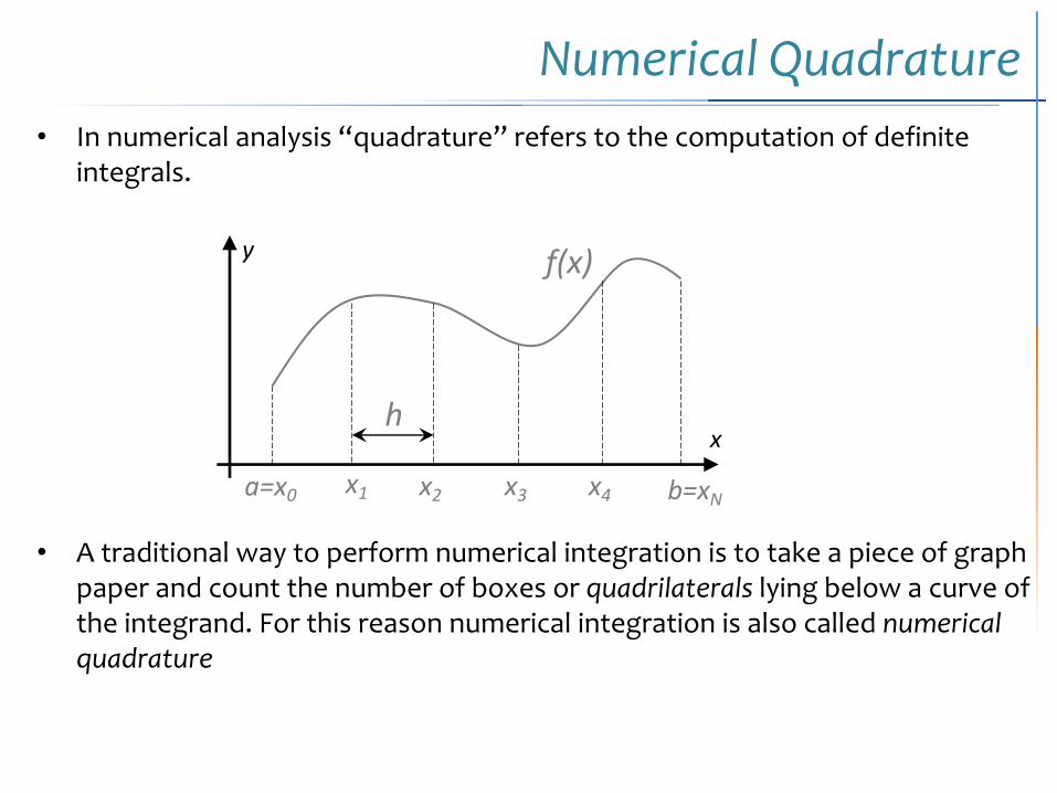
Numerical Quadrature• In numerical analysis “quadrature” refers to the computation of definite

integrals.

• A traditional way to perform numerical integration is to take a piece of graph paper and count the number of boxes or quadrilaterals lying below a curve of the integrand. For this reason numerical integration is also called numerical quadrature

h

a=x0 b=xNx1 x2 x3 x4

f(x)y

x

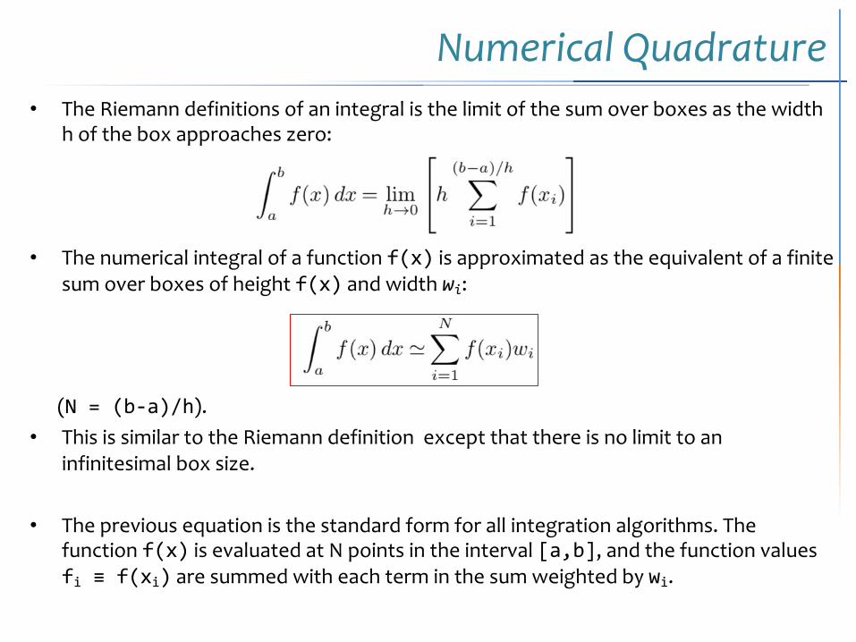
Numerical Quadrature• The Riemann definitions of an integral is the limit of the sum over boxes as the width

h of the box approaches zero:

• The numerical integral of a function f(x) is approximated as the equivalent of a finite sum over boxes of height f(x) and width wi:

(N = (b-a)/h).• This is similar to the Riemann definition except that there is no limit to an

infinitesimal box size.

• The previous equation is the standard form for all integration algorithms. The function f(x) is evaluated at N points in the interval [a,b], and the function values fi ≡ f(xi) are summed with each term in the sum weighted by wi.

Numerical Quadrature

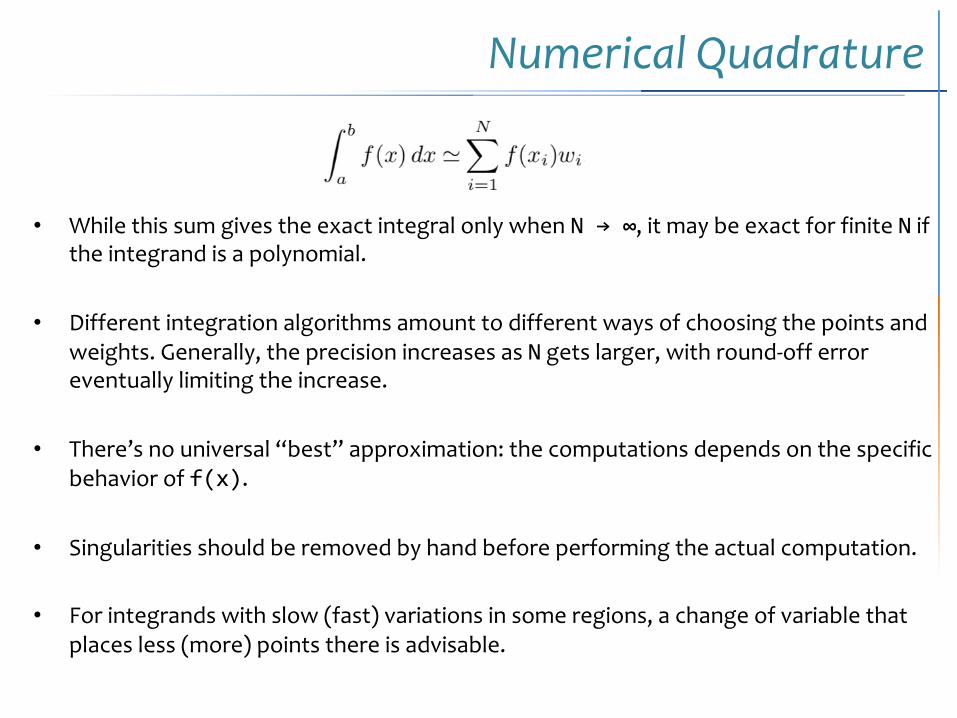
• While this sum gives the exact integral only when N → ∞, it may be exact for finite N if the integrand is a polynomial.

• Different integration algorithms amount to different ways of choosing the points and weights. Generally, the precision increases as N gets larger, with round-off error eventually limiting the increase.

• There’s no universal “best” approximation: the computations depends on the specific behavior of f(x).

• Singularities should be removed by hand before performing the actual computation.

• For integrands with slow (fast) variations in some regions, a change of variable that places less (more) points there is advisable.

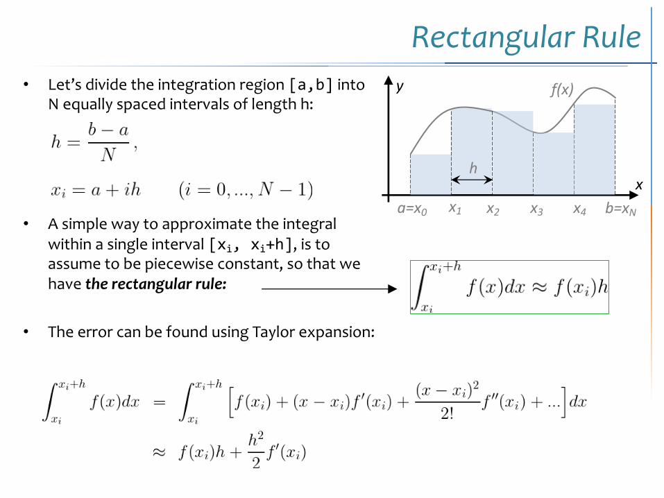
Rectangular Rule• Let’s divide the integration region [a,b] into

N equally spaced intervals of length h:

• A simple way to approximate the integral within a single interval [xi, xi+h], is to assume to be piecewise constant, so that we have the rectangular rule:

• The error can be found using Taylor expansion:

h

a=x0 b=xNx1 x2 x3 x4

f(x)y

x

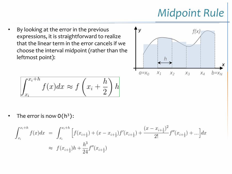
Midpoint Rule• By looking at the error in the previous

expressions, it is straightforward to realize that the linear term in the error cancels if we choose the interval midpoint (rather than the leftmost point):

• The error is now O(h3):

h

a=x0 b=xNx1 x2 x3 x4

f(x)y

x

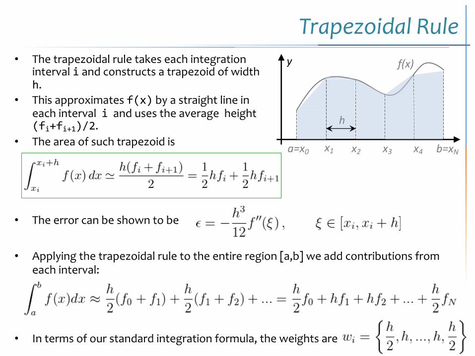
Trapezoidal Rule• The trapezoidal rule takes each integration

interval i and constructs a trapezoid of width h.

• This approximates f(x) by a straight line in each interval i and uses the average height (fi+fi+1)/2.

• The area of such trapezoid is

• The error can be shown to be

h

a=x0 b=xNx1 x2 x3 x4

f(x)y

• Applying the trapezoidal rule to the entire region [a,b] we add contributions from each interval:

• In terms of our standard integration formula, the weights are

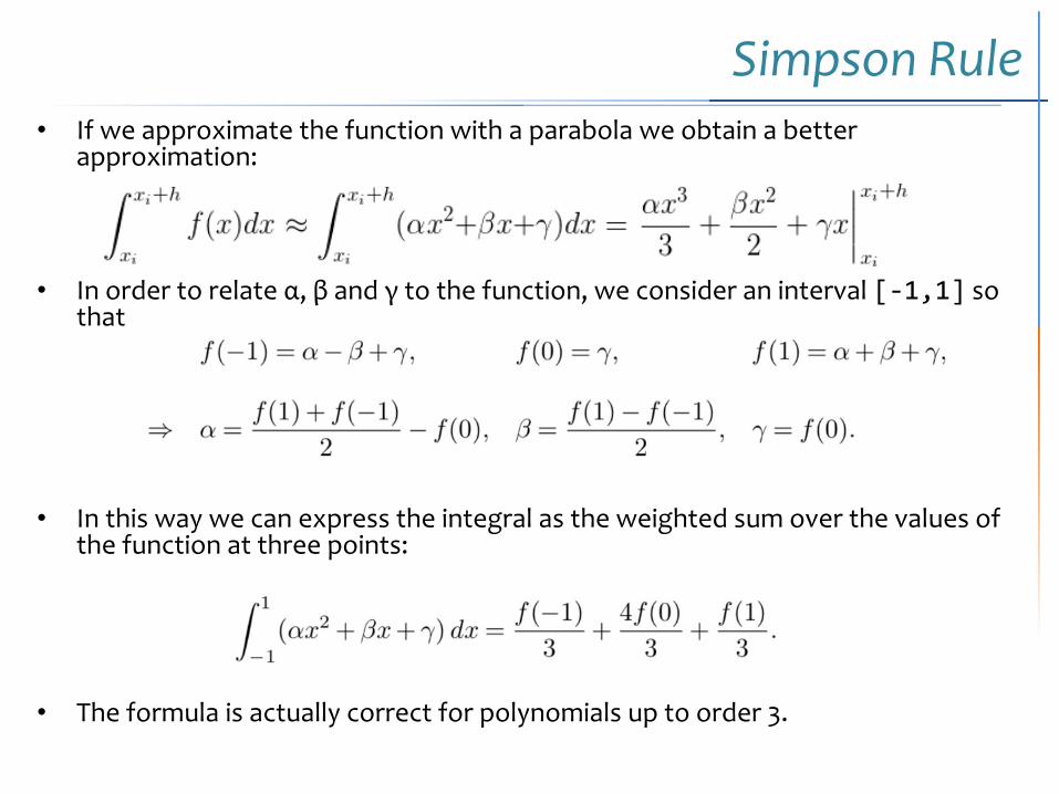
Simpson Rule• If we approximate the function with a parabola we obtain a better

approximation:

• In order to relate α, β and γ to the function, we consider an interval [-1,1] so that

• In this way we can express the integral as the weighted sum over the values of the function at three points:

• The formula is actually correct for polynomials up to order 3.

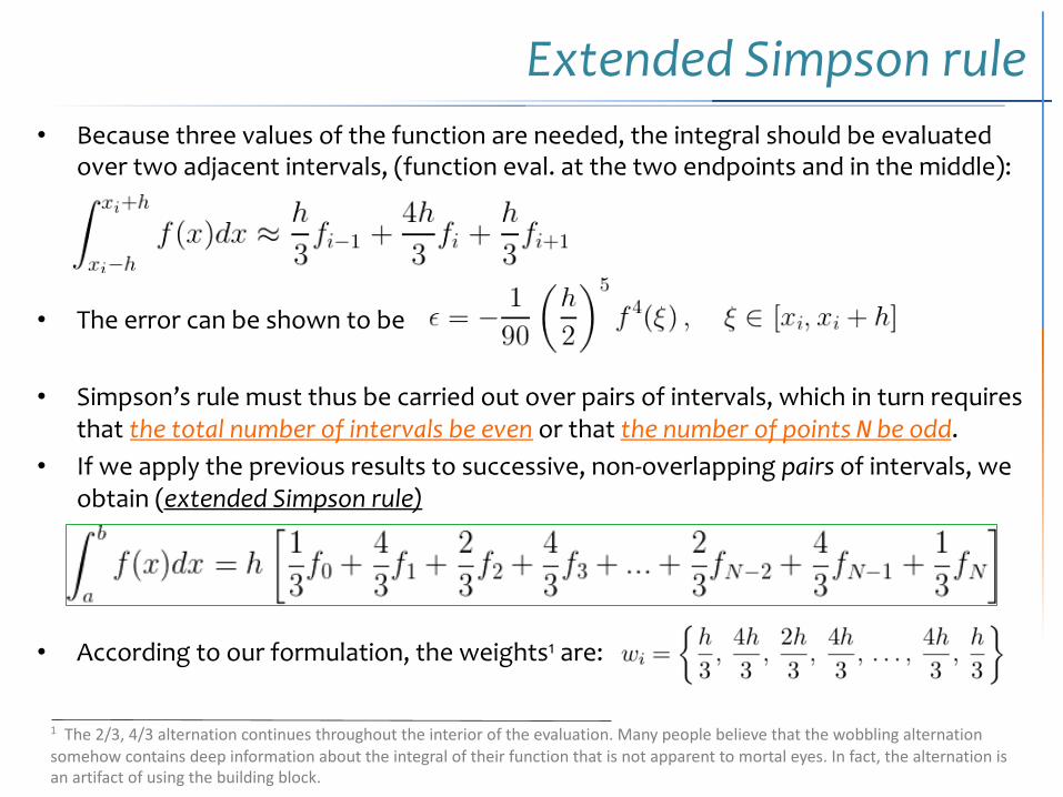
Extended Simpson rule• Because three values of the function are needed, the integral should be evaluated

over two adjacent intervals, (function eval. at the two endpoints and in the middle):

• The error can be shown to be

• Simpson’s rule must thus be carried out over pairs of intervals, which in turn requires that the total number of intervals be even or that the number of points N be odd.

• If we apply the previous results to successive, non-overlapping pairs of intervals, we obtain (extended Simpson rule)

• According to our formulation, the weights1 are:

1 The 2/3, 4/3 alternation continues throughout the interior of the evaluation. Many people believe that the wobbling alternation somehow contains deep information about the integral of their function that is not apparent to mortal eyes. In fact, the alternation is an artifact of using the building block.

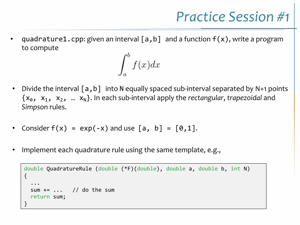
Practice Session #1• quadrature1.cpp: given an interval [a,b] and a function f(x), write a program

to compute

• Divide the interval [a,b] into N equally spaced sub-interval separated by N+1 points {x0, x1, x2, … xN}. In each sub-interval apply the rectangular, trapezoidal and Simpson rules.

• Consider f(x) = exp(-x) and use [a, b] = [0,1].

• Implement each quadrature rule using the same template, e.g.,

double QuadratureRule (double (*F)(double), double a, double b, int N) {

...sum += ... // do the sumreturn sum;

}

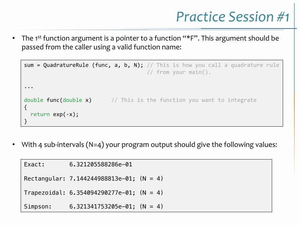
Practice Session #1• The 1st function argument is a pointer to a function “*F”. This argument should be

passed from the caller using a valid function name:

• With 4 sub-intervals (N=4) your program output should give the following values:

Exact: 6.321205588286e-01

Rectangular: 7.144244988813e-01; (N = 4)

Trapezoidal: 6.354094290277e-01; (N = 4)

Simpson: 6.321341753205e-01; (N = 4)

sum = QuadratureRule (func, a, b, N); // This is how you call a quadrature rule // from your main().

...

double func(double x) // This is the function you want to integrate{

return exp(-x);}

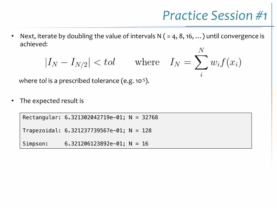
Practice Session #1• Next, iterate by doubling the value of intervals N ( = 4, 8, 16, …) until convergence is

achieved:

where tol is a prescribed tolerance (e.g. 10-5).

• The expected result is

Rectangular: 6.321302042719e-01; N = 32768

Trapezoidal: 6.321237739567e-01; N = 128

Simpson: 6.321206123892e-01; N = 16

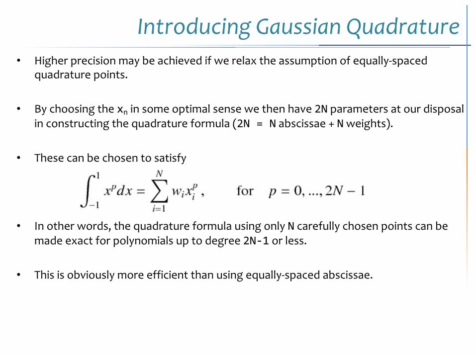
Introducing Gaussian Quadrature• Higher precision may be achieved if we relax the assumption of equally-spaced

quadrature points.

• By choosing the xn in some optimal sense we then have 2N parameters at our disposal in constructing the quadrature formula (2N = N abscissae + N weights).

• These can be chosen to satisfy

• In other words, the quadrature formula using only N carefully chosen points can be made exact for polynomials up to degree 2N-1 or less.

• This is obviously more efficient than using equally-spaced abscissae.

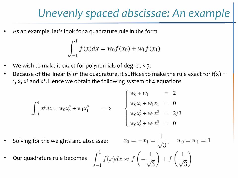
Unevenly spaced abscissae: An example• As an example, let’s look for a quadrature rule in the form

• We wish to make it exact for polynomials of degree ≤ 3.• Because of the linearity of the quadrature, it suffices to make the rule exact for f(x) =

1, x, x2 and x3. Hence we obtain the following system of 4 equations

• Solving for the weights and abscissae:

• Our quadrature rule becomes

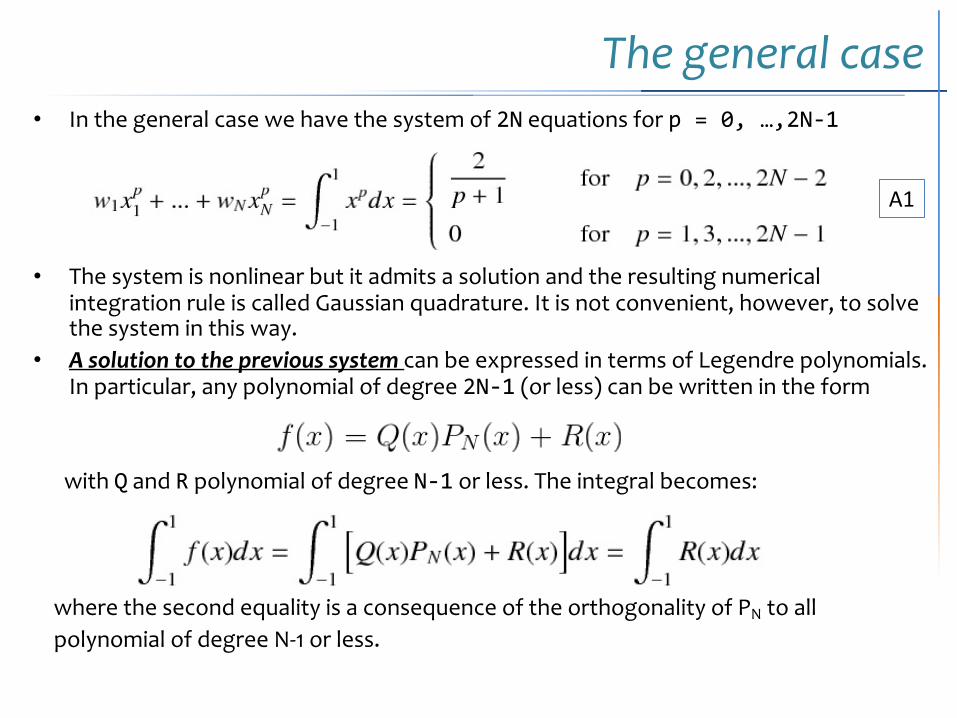
The general case• In the general case we have the system of 2N equations for p = 0, …,2N-1

• The system is nonlinear but it admits a solution and the resulting numerical integration rule is called Gaussian quadrature. It is not convenient, however, to solve the system in this way.

• A solution to the previous system can be expressed in terms of Legendre polynomials. In particular, any polynomial of degree 2N-1 (or less) can be written in the form

with Q and R polynomial of degree N-1 or less. The integral becomes:

where the second equality is a consequence of the orthogonality of PN to all polynomial of degree N-1 or less.

A1

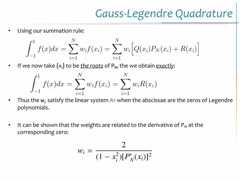
Gauss-Legendre Quadrature• Using our summation rule:

• If we now take {xi} to be the roots of PN, the we obtain exactly:

• Thus the wi satisfy the linear system A1 when the abscissae are the zeros of Legendre polynomials.

• It can be shown that the weights are related to the derivative of PN at the corresponding zero:

Gauss-Legendre Quadrature: a note• As a general rule, Gaussian quadrature is the method of choice when the integrand is

known analytically, smooth or it can be made smooth enough by extracting from it a function that is the weight for a standard set of orthogonal polynomials.

• One has to evaluate weights and abscissae.

• If the integrand varies rapidly, we can repeat the basic Gaussian quadrature formula by applying it over several sub-intervals in the range of integration.

• Finally, if the integrand can be evaluated only at equally-spaced abscissae (for example when it is generated by integrating a differential equation), then Simpson (or higher) formula should be used.

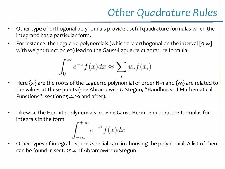
Other Quadrature Rules• Other type of orthogonal polynomials provide useful quadrature formulas when the

integrand has a particular form. • For instance, the Laguerre polynomials (which are orthogonal on the interval [0,∞]

with weight function e-x) lead to the Gauss-Laguerre quadrature formula:

• Here {xi} are the roots of the Laguerre polynomial of order N+1 and {wi} are related to the values at these points (see Abramowitz & Stegun, “Handbook of Mathematical Functions”, section 25.4.29 and after).

• Likewise the Hermite polynomials provide Gauss-Hermite quadrature formulas for integrals in the form

• Other types of integral requires special care in choosing the polynomial. A list of them can be found in sect. 25.4 of Abramowitz & Stegun.

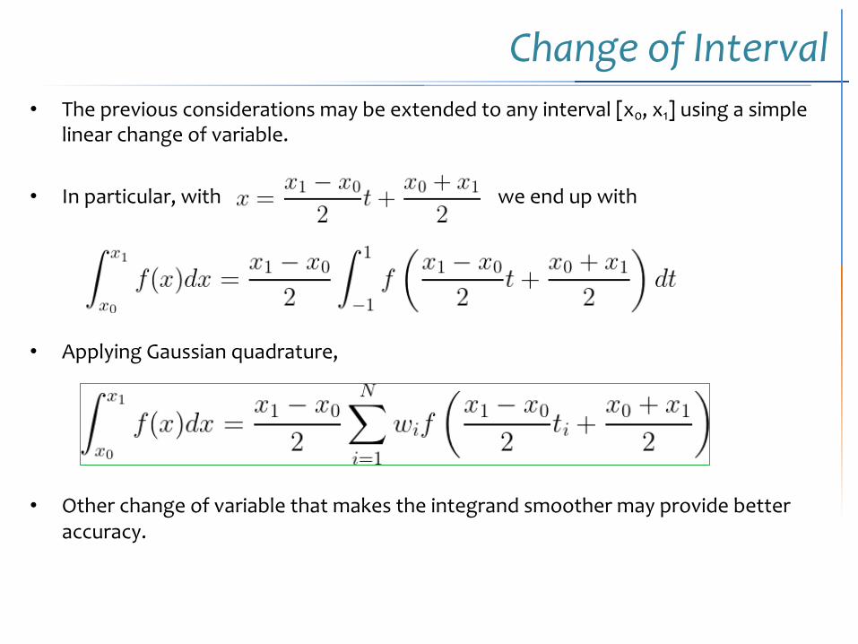
Change of Interval• The previous considerations may be extended to any interval [x0, x1] using a simple

linear change of variable.

• In particular, with we end up with

• Applying Gaussian quadrature,

• Other change of variable that makes the integrand smoother may provide better accuracy.

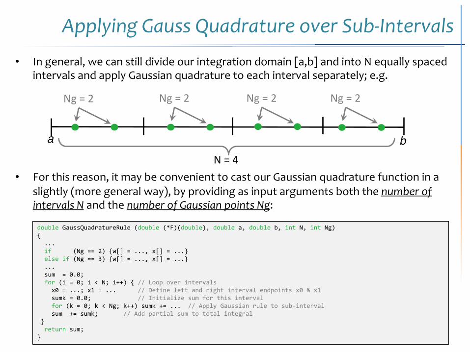
Applying Gauss Quadrature over Sub-Intervals

• In general, we can still divide our integration domain [a,b] and into N equally spaced intervals and apply Gaussian quadrature to each interval separately; e.g.

• For this reason, it may be convenient to cast our Gaussian quadrature function in a slightly (more general way), by providing as input arguments both the number of intervals N and the number of Gaussian points Ng:

double GaussQuadratureRule (double (*F)(double), double a, double b, int N, int Ng) {...if (Ng == 2) {w[] = ..., x[] = ...}else if (Ng == 3) {w[] = ..., x[] = ...}... sum = 0.0;for (i = 0; i < N; i++) { // Loop over intervals

x0 = ...; x1 = ... // Define left and right interval endpoints x0 & x1sumk = 0.0; // Initialize sum for this interval for (k = 0; k < Ng; k++) sumk += ... // Apply Gaussian rule to sub-intervalsum += sumk; // Add partial sum to total integral

}return sum;

}

N = 4

Ng = 2 Ng = 2 Ng = 2 Ng = 2

a b

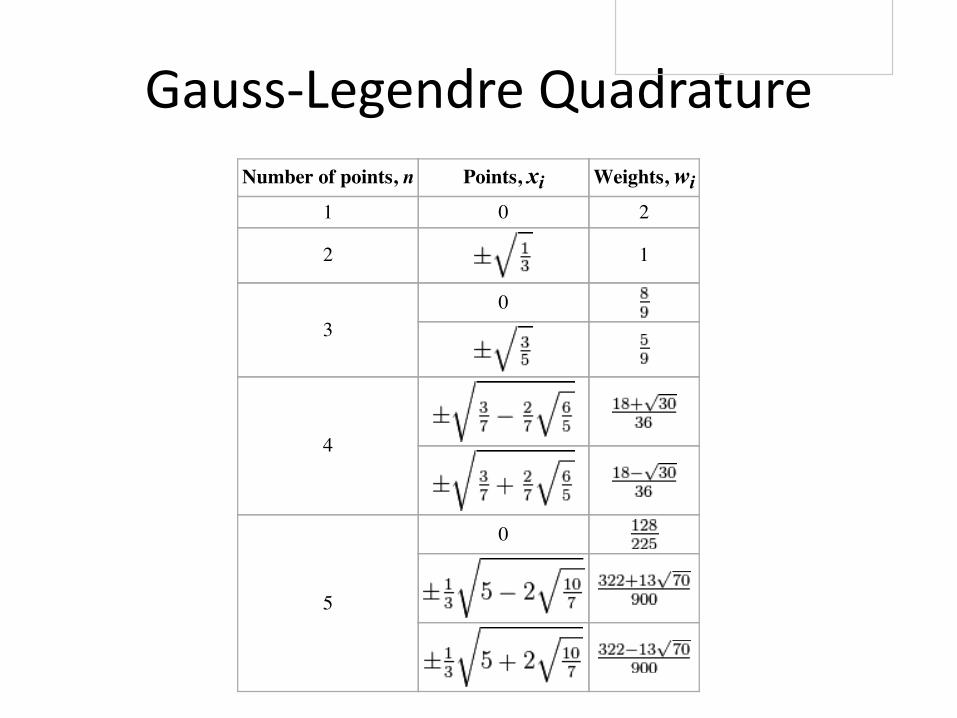
Gauss-Legendre QuadratureGraphs of Legendre polynomials (upto n = 5)

For the simplest integration problem stated above, i.e. with , the associated polynomials are Legendre polynomials,

Pn(x), and the method is usually known as Gauss–Legendrequadrature. With the n-th polynomial normalized to give Pn(1) = 1,the i-th Gauss node, xi, is the i-th root of Pn; its weight is given by(Abramowitz & Stegun 1972, p. 887)

Some low-order rules for solving the integration problem are listedbelow.

Number of points, n Points, xi Weights, wi1 0 2

2 1

30

4

5

0

Change of interval

An integral over [a,  b] must be changed into an integral over [−1,  1] before applying the Gaussianquadrature rule. This change of interval can be done in the following way:

Applying the Gaussian quadrature rule then results in the following approximation:

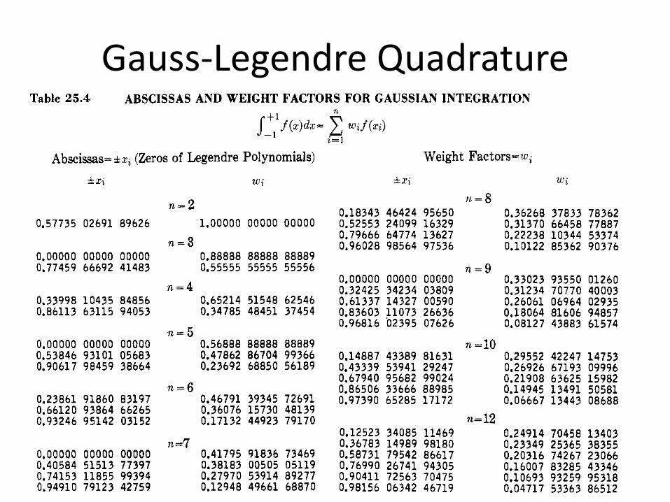
916 NUMERICAL ANALYSIS

ABSCISSAS AND WEIGHT FACTORS FOR GAUSSIAN INTEGRATION Table 25.4

U 2= I

Abscissas= iti (Zeros of Legendre Polynomials) i xi 'U) i

n = 2 0.57735 02691 89626 1.00000 00000 00000

0.00000 00000 00000 0.88888 88888 88889 0.77459 66692 41483 0.55555 55555 55556

n = 4 0.33998 10435 84856 0.65214 51548 62546 0.86113 63115 94053 0.34785 48451 37454

n = 3

Weight Factors=wi +xi wi

I1 = 8 0.18343 46424 95650 0.52553 24099 16329 0.79666 64774 13627 0.96028 98564 97536

0.36268 37833 78362 0.31370 66458 77887 0.22238 10344 53374 0.10122 85362 90376

n = 9 0.33023 93550 01260 0.31234 70770 40003

0.00000 00000 00000 0.32425 34234 03809 0.61337 14327 00590 0.83603 11073 26636 0.96816 b2395 07626

0.26061 06964 02935 0.18064 81606 94857 0.08127 43883 61574 .n=5

0.00000 00000 00000 0.56888 88888 88889 0.53846 93101 05683 0.47862 86704 99366 0.90617 98459 38664 0.23692 68850 56189

n =10 0.14887 43389 81631 0.43339 53941 29247 0.67940 95682 99024

0.29552 42247 14753 0.26926 67193 09996 0.21908 63625 15982 0.14945 13491 50581 0.06667 13443 08688

n = 6 0.86506 33666 88985 0.97390 65285 17172 0.23861 91860 83197 0.46791 39345 72691

0.66120 93864 66265 0.36076 15730 48139 0.93246 95142 03152 0.17132 44923 79170 n= 12

0.24914 70458 13403 0.23349 25365 38355 0.20316 74267 23066 0.16007 83285 43346 0.10693 93259 95318 0.04717 53363 86512

0.12523 34085 11469 0.36783 14989 98180 0.58731 79542 86617 0.76990 26741 94305 0.90411 72563 70475 0.98156 06342 46719

n 2 7 .. . 0.00000 00000 00000 0.41795 91836 73469 0.40584 51513 77397 0.38183 00505 05119 0.74153 11855 99394 0.27970 53914 89277 0.94910 79123 42759 0.12948 49661 68870

U' i 0.18945 06104 5

i xi n= 16 0.09501 25098 37637 440185 0.28160 35507 79258 913230 0.45801 67776 57227 386342 0.61787 62444 02643 748447 0.75540 44083 55003 033895 0.86563 12023 87831 743880

068 923 002 576

55533 82492 38647 11754

496285 588867 538189 732081 872052 784810 892863 094852

Oil8260 34150 $ 0.16915 65193 , 0.14959 59888 1 0.12462 0.09515 0.06225 0.02715

89712 85116 35239 24594

0.94457 50230 73232 576078 0.98940 09349 91649 932596

0.07652 65211 33497 333755 0.22778 58511 41645 078080 0.37370 60887 15419 560673 0.51086 70019 50827 098004 0.63605 36807 26515 025453 0.74633 19064 60150 792614 0.83911 69718 22218 823395 0.91223 44282 51325 905868 0.96397 19272 77913 791268 0.99312 85991 85094 924786

0.15275 33871 30725 850698 0.14917 29864 72603 746788 0.14209 61093 18382 051329 0.13168 86384 49176 626898 0.11819 45319 61518 417312 0.10193 01198 17240 435037 0.08327 67415 76704 748725 Oi06267 20483 34109 063570 0.04060 14298 00386 941331 0.01761 40071 39152 118312

n=24 0.06405 68928 62605 626085 0.19111 88674 73616 309159 0.31504 26796 96163 374387 0.43379 35076 26045 138487 0.54542 14713 88839 535658 0.64809 36519 36975 569252 0.74012 41915 78554 364244 0.82000 19859 73902 921954 0.88641 55270 04401 034213 0.93827 45520 02732 758524 0.97472 85559 71309 498198 0.99518 72199 97021 360180

0.12793 81953 46752 156974 0.12583 74563 46828 296121 0.12167 04729 27803 91204 0.11550 56680 53725 6 1353 0.10744 42701 15965 63 's, 783 0.09761 86521 04113 888270 0.08619 01615 31953 275917 0.07334 64814 11080 305734 0.05929 85849 15436 780746 0.04427 74388 17419 806169 0.02853 13886 28933 663181 0.01234 12297 99987 199547

Compiled from P. Davis and P. Rabinowitz, Abscissas and weights for Gaussian quadratures of high order, J. Research NBS 56, 35-37, 1956, RP2645; P. Davis and P. Rabinowitz, Additional abscissas and weights for Gaussian quadratures of high order. Values for n=64, 80, and 96, J. Research NBS 60, 613-614,1958, RP2875; and A. N. Lowan, N. Davids, and A. Levenson, Table of the zeros of the Legendre polynomials of order 1-16 and the weight coefficients for Gauss' mechanical quadrature formula, Bull. Amer. Math. Soc. 48, 739-743, 1942 (with permission).

Gauss-Legendre Quadrature

Other forms

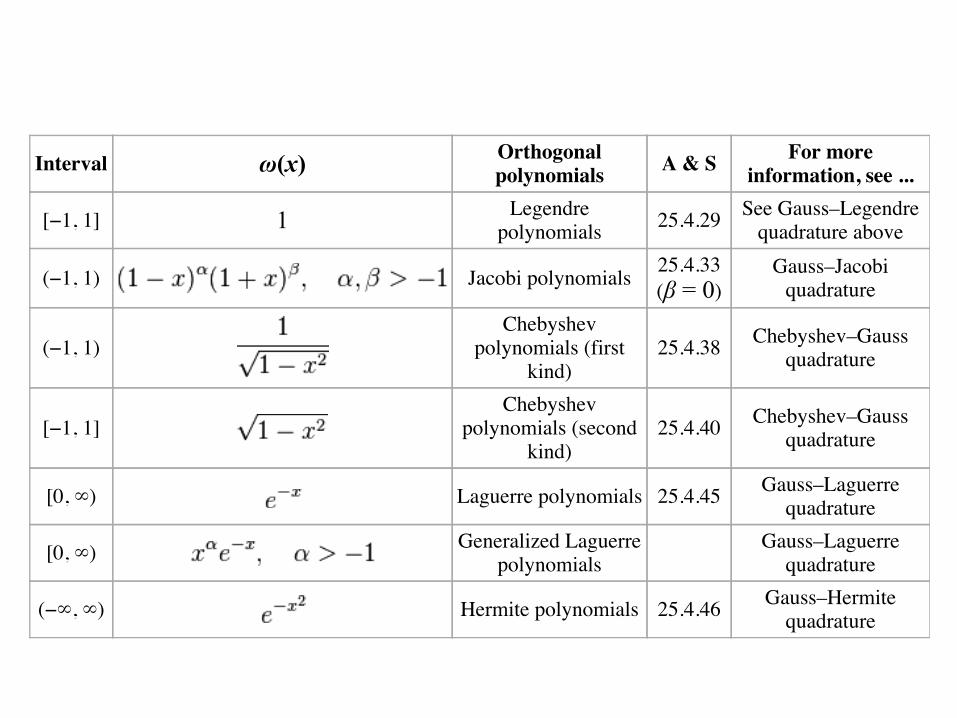
The integration problem can be expressed in a slightly more general way by introducing a positive weightfunction ω into the integrand, and allowing an interval other than [−1,  1]. That is, the problem is tocalculate

for some choices of a, b, and ω. For a = −1, b = 1, and ω(x) = 1, the problem is the same as thatconsidered above. Other choices lead to other integration rules. Some of these are tabulated below.Equation numbers are given for Abramowitz and Stegun (A & S).

Interval ω(x) Orthogonal

polynomialsA & S

For more

information, see ...

[−1, 1] 1 Legendrepolynomials 25.4.29 See Gauss–Legendre

quadrature above

(−1, 1) Jacobi polynomials 25.4.33(β  =  0)

Gauss–Jacobiquadrature

(−1, 1)Chebyshev

polynomials (firstkind)

25.4.38 Chebyshev–Gaussquadrature

[−1, 1]Chebyshev

polynomials (secondkind)

25.4.40 Chebyshev–Gaussquadrature

[0, ∞) Laguerre polynomials 25.4.45 Gauss–Laguerrequadrature

[0, ∞) Generalized Laguerrepolynomials

Gauss–Laguerrequadrature

(−∞, ∞) Hermite polynomials 25.4.46 Gauss–Hermitequadrature

Fundamental theorem

Let pn be a nontrivial polynomial of degree n such that

If we pick the n nodes xi to be the zeros of pn, then there exist n weights wi which make the Gauss-quadrature computed integral exact for all polynomials h(x) of degree 2n − 1 or less. Furthermore, allthese nodes xi will lie in the open interval (a, b) (Stoer & Bulirsch 2002, pp. 172–175).

The polynomial pn is said to be an orthogonal polynomial of degree n associated to the weight functionω(x). It is unique up to a constant normalization factor. The idea underlying the proof is that, because ofits sufficiently low degree, h(x) can be divided by to produce a quotient q(x) of degree strictlylower than n, and a remainder r(x) of still lower degree, so that both will be orthogonal to , by thedefining property of . Thus

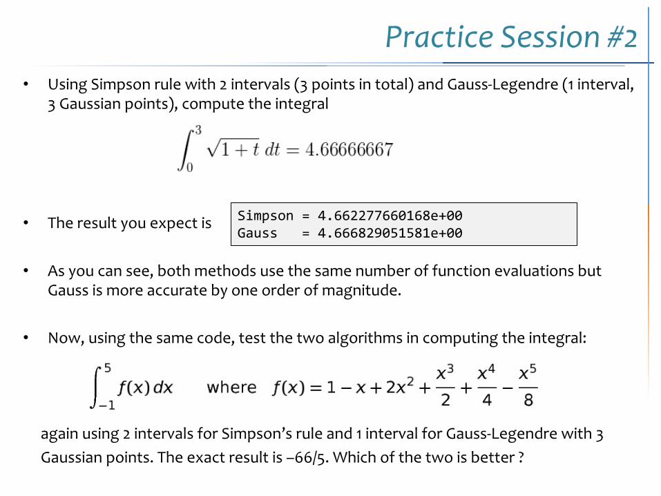
Practice Session #2• Using Simpson rule with 2 intervals (3 points in total) and Gauss-Legendre (1 interval,

3 Gaussian points), compute the integral

• The result you expect is

• As you can see, both methods use the same number of function evaluations but Gauss is more accurate by one order of magnitude.

• Now, using the same code, test the two algorithms in computing the integral:

again using 2 intervals for Simpson’s rule and 1 interval for Gauss-Legendre with 3 Gaussian points. The exact result is –66/5. Which of the two is better ?

Simpson = 4.662277660168e+00Gauss = 4.666829051581e+00

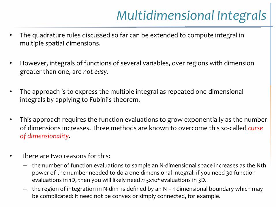
Multidimensional Integrals• The quadrature rules discussed so far can be extended to compute integral in

multiple spatial dimensions.

• However, integrals of functions of several variables, over regions with dimension greater than one, are not easy.

• The approach is to express the multiple integral as repeated one-dimensional integrals by applying to Fubini's theorem.

• This approach requires the function evaluations to grow exponentially as the number of dimensions increases. Three methods are known to overcome this so-called curse of dimensionality.

• There are two reasons for this:– the number of function evaluations to sample an N-dimensional space increases as the Nth

power of the number needed to do a one-dimensional integral: if you need 30 function evaluations in 1D, then you will likely need ≈ 3x104 evaluations in 3D.

– the region of integration in N-dim is defined by an N − 1 dimensional boundary which may be complicated: it need not be convex or simply connected, for example.

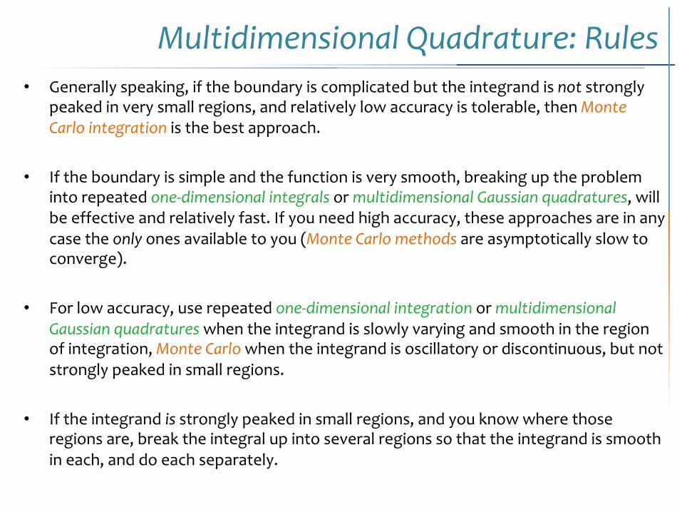
Multidimensional Quadrature: Rules• Generally speaking, if the boundary is complicated but the integrand is not strongly

peaked in very small regions, and relatively low accuracy is tolerable, then Monte Carlo integration is the best approach.

• If the boundary is simple and the function is very smooth, breaking up the problem into repeated one-dimensional integrals or multidimensional Gaussian quadratures, will be effective and relatively fast. If you need high accuracy, these approaches are in any case the only ones available to you (Monte Carlo methods are asymptotically slow to converge).

• For low accuracy, use repeated one-dimensional integration or multidimensional Gaussian quadratures when the integrand is slowly varying and smooth in the region of integration, Monte Carlo when the integrand is oscillatory or discontinuous, but not strongly peaked in small regions.

• If the integrand is strongly peaked in small regions, and you know where those regions are, break the integral up into several regions so that the integrand is smooth in each, and do each separately.

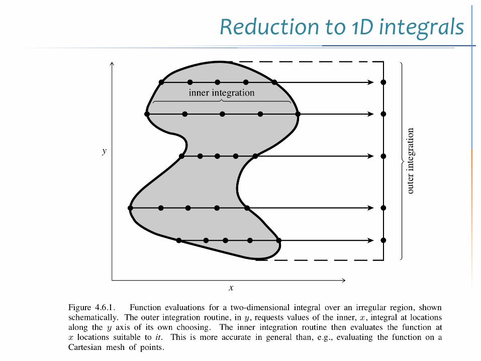
Reduction to 1D integrals

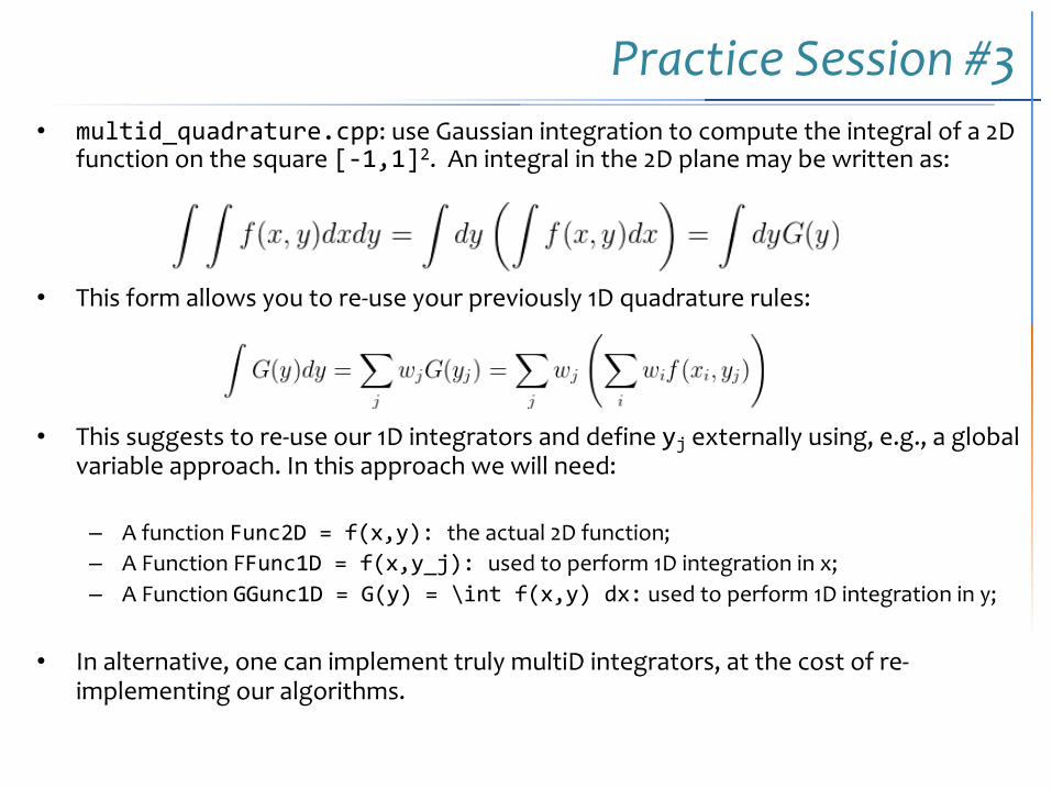
Practice Session #3• multid_quadrature.cpp: use Gaussian integration to compute the integral of a 2D

function on the square [-1,1]2. An integral in the 2D plane may be written as:

• This form allows you to re-use your previously 1D quadrature rules:

• This suggests to re-use our 1D integrators and define yj externally using, e.g., a global variable approach. In this approach we will need:

– A function Func2D = f(x,y): the actual 2D function;– A Function FFunc1D = f(x,y_j): used to perform 1D integration in x;– A Function GGunc1D = G(y) = \int f(x,y) dx: used to perform 1D integration in y;

• In alternative, one can implement truly multiD integrators, at the cost of re-implementing our algorithms.

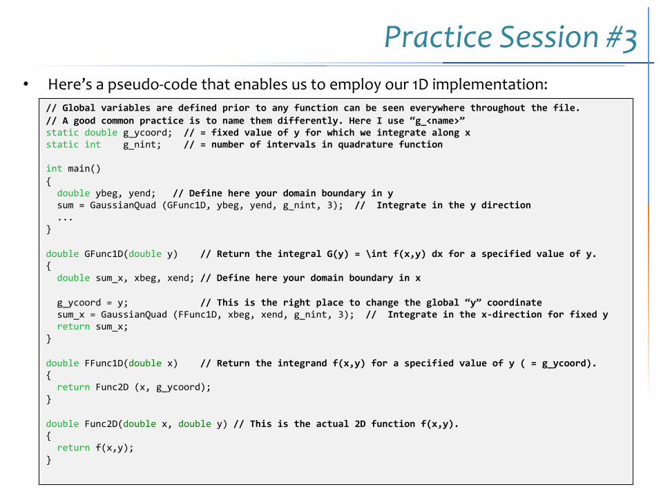
Practice Session #3• Here’s a pseudo-code that enables us to employ our 1D implementation:

// Global variables are defined prior to any function can be seen everywhere throughout the file.// A good common practice is to name them differently. Here I use “g_<name>”static double g_ycoord; // = fixed value of y for which we integrate along xstatic int g_nint; // = number of intervals in quadrature function

int main(){double ybeg, yend; // Define here your domain boundary in ysum = GaussianQuad (GFunc1D, ybeg, yend, g_nint, 3); // Integrate in the y direction...

}

double GFunc1D(double y) // Return the integral G(y) = \int f(x,y) dx for a specified value of y.{double sum_x, xbeg, xend; // Define here your domain boundary in x

g_ycoord = y; // This is the right place to change the global “y” coordinatesum_x = GaussianQuad (FFunc1D, xbeg, xend, g_nint, 3); // Integrate in the x-direction for fixed yreturn sum_x;

}

double FFunc1D(double x) // Return the integrand f(x,y) for a specified value of y ( = g_ycoord).{return Func2D (x, g_ycoord);

}

double Func2D(double x, double y) // This is the actual 2D function f(x,y).{return f(x,y);

}

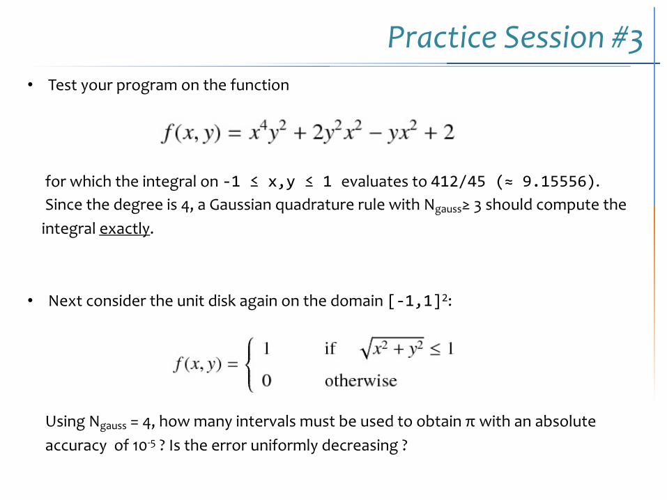
Practice Session #3• Test your program on the function

for which the integral on -1 ≤ x,y ≤ 1 evaluates to 412/45 (≈ 9.15556). Since the degree is 4, a Gaussian quadrature rule with Ngauss≥ 3 should compute the integral exactly.

• Next consider the unit disk again on the domain [-1,1]2:

Using Ngauss = 4, how many intervals must be used to obtain π with an absolute accuracy of 10-5 ? Is the error uniformly decreasing ?

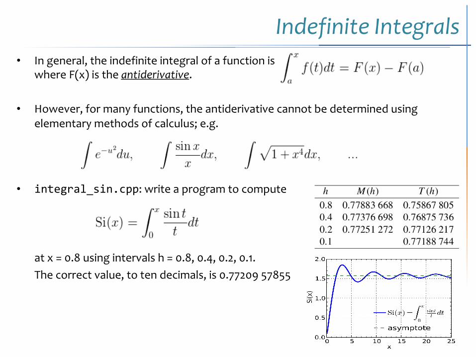
Indefinite Integrals• In general, the indefinite integral of a function is

where F(x) is the antiderivative.

• However, for many functions, the antiderivative cannot be determined using elementary methods of calculus; e.g.

• integral_sin.cpp: write a program to compute

at x = 0.8 using intervals h = 0.8, 0.4, 0.2, 0.1. The correct value, to ten decimals, is 0.77209 57855

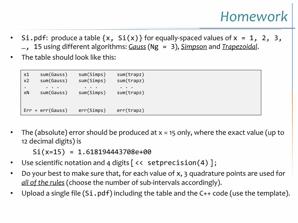
Homework• Si.pdf: produce a table {x, Si(x)} for equally-spaced values of x = 1, 2, 3,

…, 15 using different algorithms: Gauss (Ng = 3), Simpson and Trapezoidal.• The table should look like this:

• The (absolute) error should be produced at x = 15 only, where the exact value (up to 12 decimal digits) is

Si(x=15) = 1.618194443708e+00 • Use scientific notation and 4 digits [ << setprecision(4) ] ;• Do your best to make sure that, for each value of x, 3 quadrature points are used for

all of the rules (choose the number of sub-intervals accordingly).• Upload a single file (Si.pdf) including the table and the C++ code (use the template).

x1 sum(Gauss) sum(Simps) sum(trapz) x2 sum(Gauss) sum(Simps) sum(trapz) . . . . . . . . . . xN sum(Gauss) sum(Simps) sum(trapz)

Err = err(Gauss) err(Simps) err(trapz)