arX

iv:p

hysi

cs/0

1050

17v4

[ph

ysic

s.pl

asm

-ph]

26

Apr

200

2

Two-surface wave decay

Andrea Macchi∗, Fulvio Cornolti and Francesco Pegoraro

Dipartimento di Fisica, Universita di Pisa e

Istituto Nazionale Fisica della Materia (INFM), sezione A,

Piazza Torricelli 2, I-56100 Pisa, Italy

Abstract

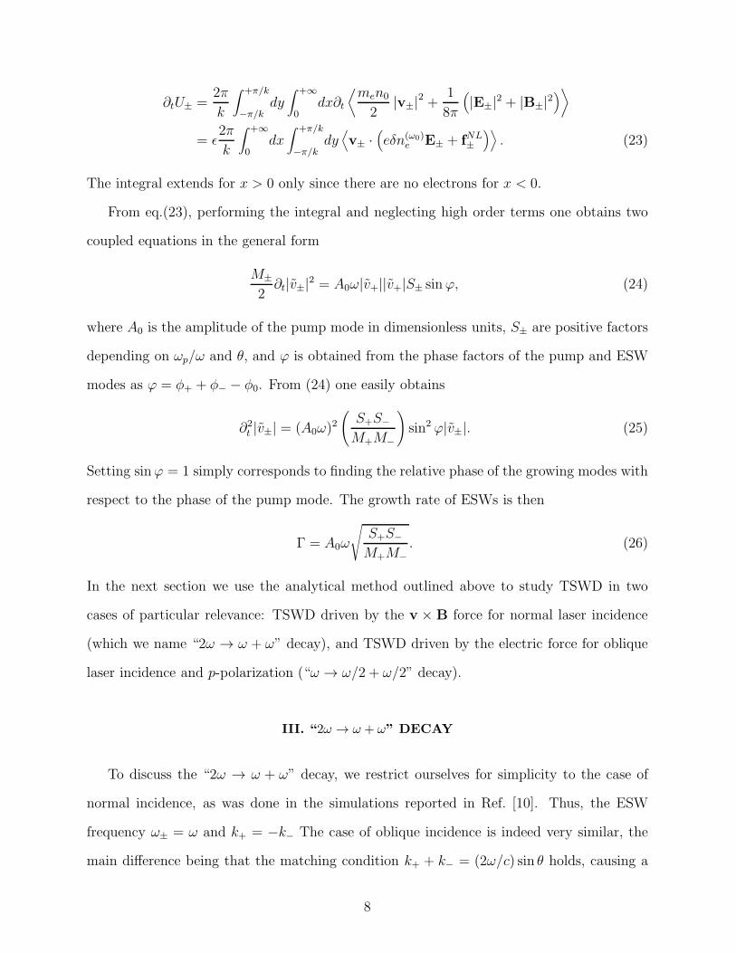
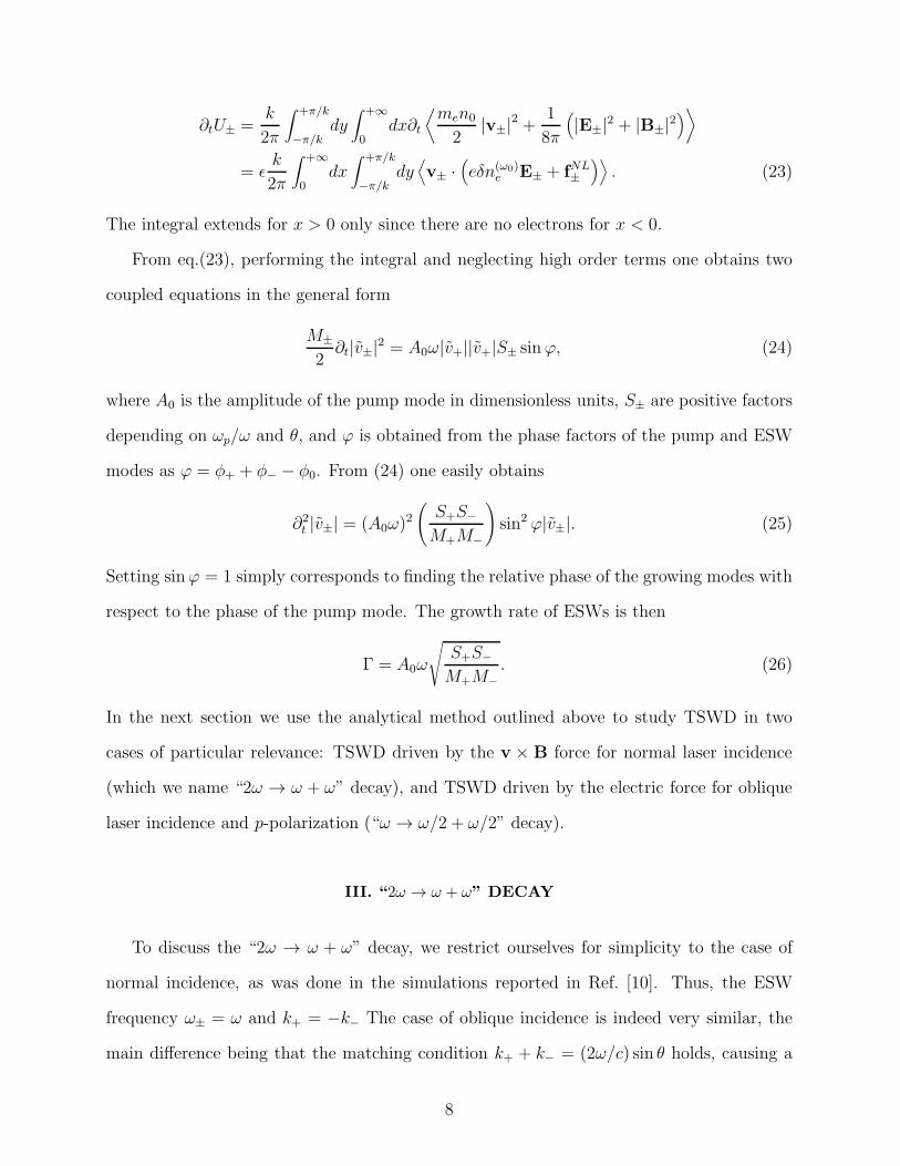
The parametric excitation of pairs of electron surface waves (ESW) in the

interaction of an ultrashort, intense laser pulse with an overdense plasma

is discussed using an analytical model. The plasma has a simple step-like

density profile. The ESWs can be excited either by the electric or by the

magnetic part of the Lorentz force exerted by the laser and, correspondingly,

have frequencies around ω/2 or ω, where ω is the laser frequency.

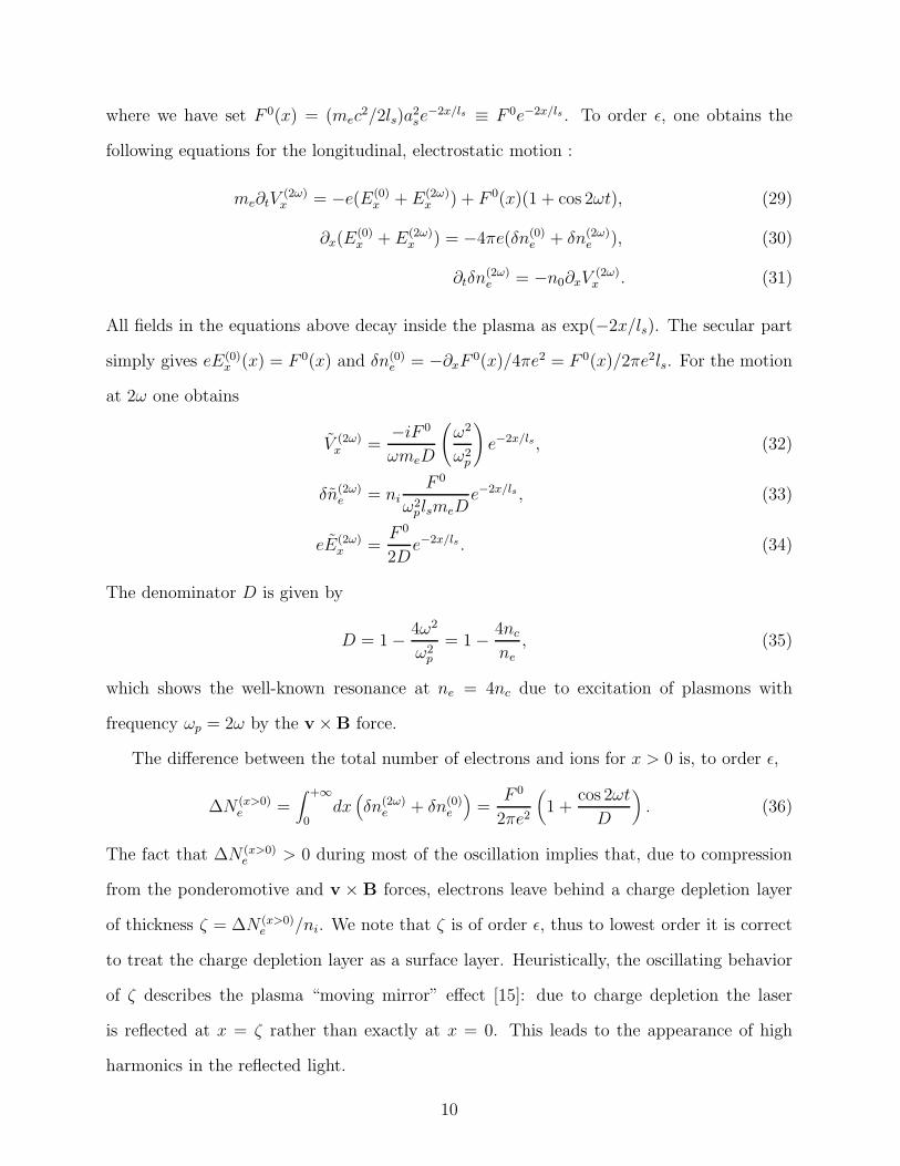
Typeset using REVTEX

∗E-mail: macchi@df.unipi.it

1

I. INTRODUCTION

Surface wave (SW) excitation has been widely studied in the past as a mechanism for

electromagnetic (EM) wave absorption in highly inhomogeneous plasmas in several regimes

and for different target geometries [1,2] and, more recently, in the specific case of solid

targets irradiated by intense, ultrashort laser pulses [3,4]. The key problem in the linear

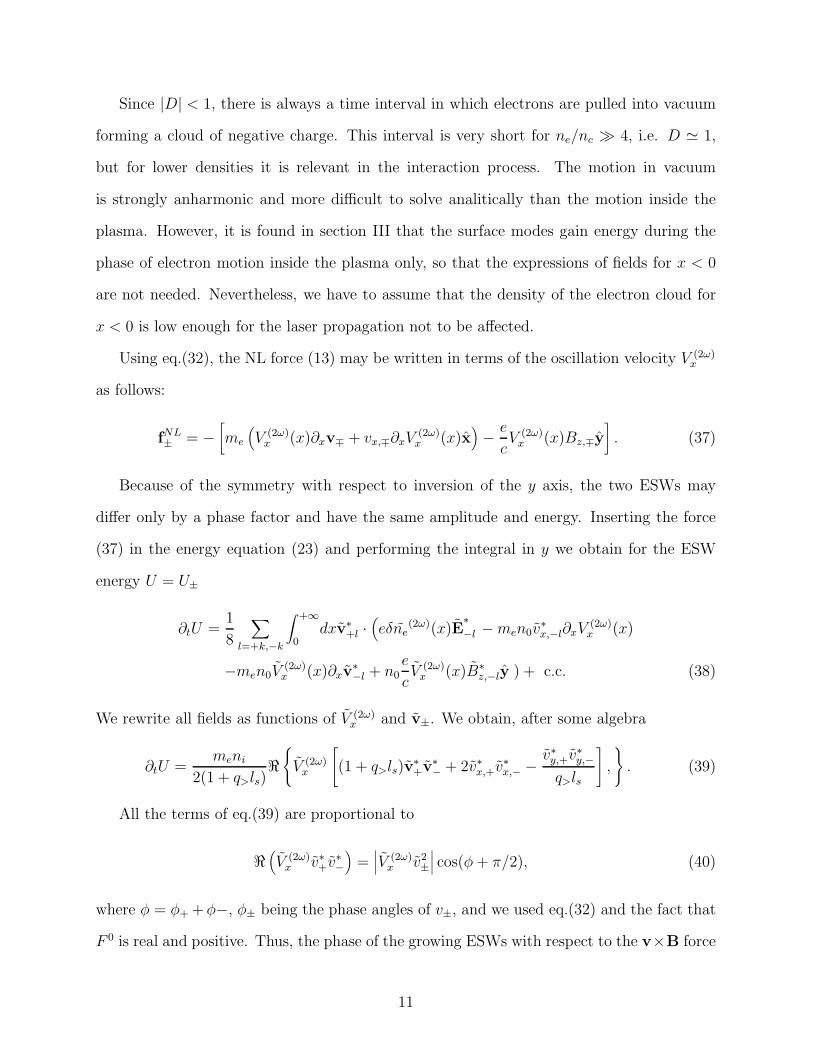
mode conversion of the EM wave (the laser pulse) into an SW of the same frequency ω is

that the phase matching between the two waves is not possible at a simple plasma-vacuum

interface. The reason for this is that for an SW vave the wavevector along the plasma surface

ks is larger than ω/c, and thus cannot be equal to the component of the EM wavevector in

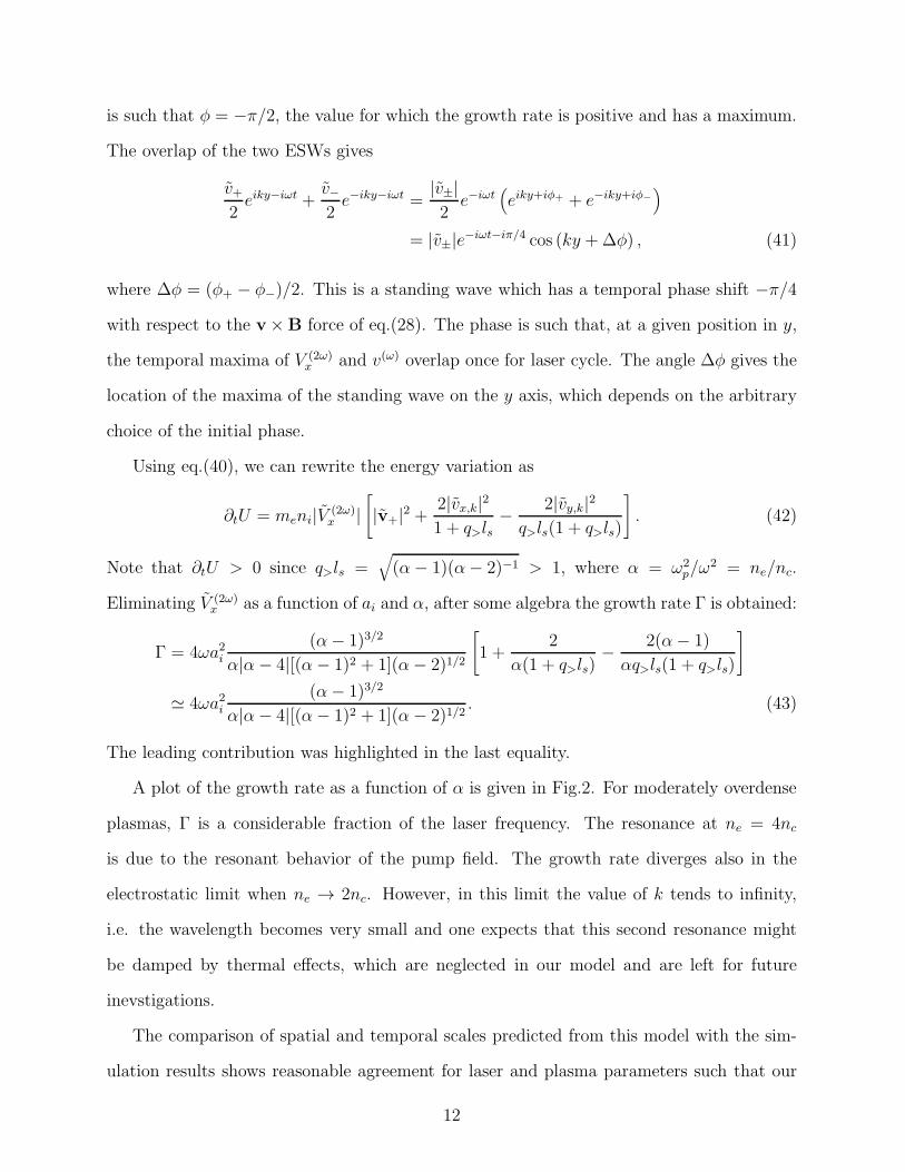
the same direction kt = (ω/c) sin θ, where θ is the incidence angle of the laser pulse. Linear

mode conversion of the laser pulse into an SW is possible in specifically tailored density

profiles, e.g. for a “double-step” density profile (i.e. at the interface between an underdense

plasma region where ω > ωp and an overdense region where ω < ωp, with ωp the plasma

frequency), or if a periodic surface modulation with wavevector kp = kt − ks exists, such

that the matching condition for the wavevectors is

kt = ks + kp. (1)

In practical applications, corrugated targets are used to optimize SW generation at a given

incidence angle. Other possible schemes of SW excitation are discussed, e.g., in Refs. [2,3].

In this paper, we discuss a different mechanism of electron surface wave (ESW) excitation

by ultrashort laser pulses, based on the generation of two counterpropagating ESWs. The

basic idea is as follows. An intense laser pulse impinging on an overdense, step-boundary

plasma drives electron oscillations at the frequencies ω and 2ω by the electric and the

magnetic part of the Lorentz force , respectively. The electron response may be viewed as

a superposition of “forced” surface modes with frequency ω0 = ω or 2ω, respectively, and

wavevector k0 = (ω0/c) sin θ. Each of these forced modes may “decay” parametrically into

two ESWs (labeled “+” and “−”, respectively) provided that the matching conditions for a

three-wave process hold:

2

k0 = k+ + k−, (2)

ω0 = ω+ + ω−. (3)

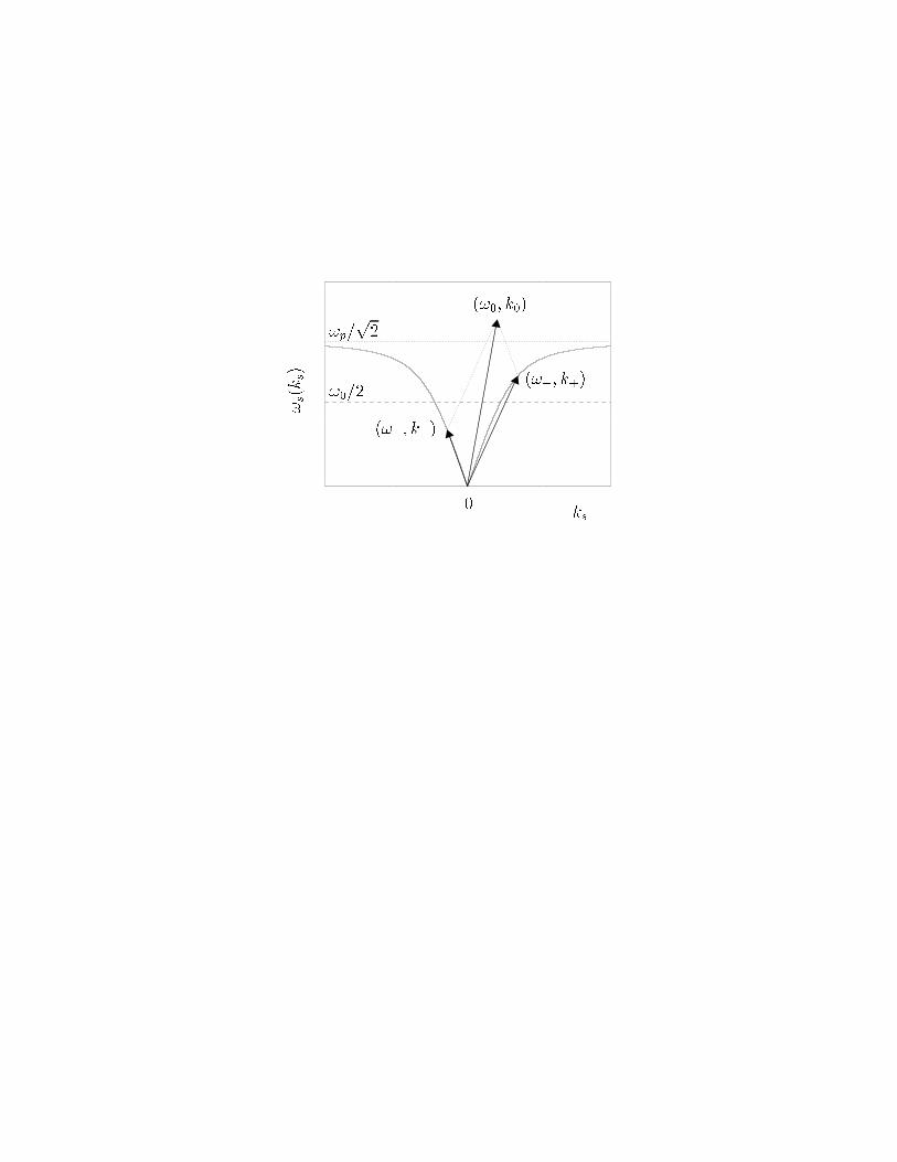
No pre-imposed target modulation is required to satisfy these relations, as depicted in Fig.1.

The ESW frequencies may be written as ω± = ω0/2 ± δω. Thus, the “decay” of the mode

excited by the electric (magnetic) force leads to the generations of ESWs with frequencies

around ω/2 (ω). We call this process “two-surface wave decay” (TSWD) in analogy to the

well-known “two-plasmon decay” parametric instability in laser-plasma interactions.

Earlier investigations of parametric and three-wave nonlinear processes involving ESWs

have been previously carried out in different regimes [5,6]. In particular, the parametric

excitation of pairs of subharmonic ESWs in a magnetized plasma by an external EM wave

was studied in Refs. [7]. These studies were restricted to the electrostatic limit in which

the ESW frequency is ωs ≃ ωp/√2 (see [8] and eq.(11) below) and does not depend on

the wavevector ks in a semi-infinite, step boundary plasma (e.g. with a density profile

ni = niΘ(x), where Θ(x) is the Heaviside step function). In the electrostatic limit the phase

matching with an impinging EM wave is possible only for particular target geometries where

the frequency of electrostatic SWs depends on ks (e.g. a plasma slab of thickness d where ωs

depends on the product ksd [5]). In our model, we assume a semi-infinite geometry but we do

not use the electrostatic approximation, and therefore in general the frequency ωs of ESWs is

significantly lower than ωp/√2 and depends on ks, approaching the EM limit ωs ≃ ksc when

ωs → 0. This allows the matching conditions (3) to be satisfied in a semi-infinite plasma.

It is interesting to notice that in Ref. [9] it has been shown that two counterpropagating

ESWs generate nonlinear radiation at a frequency that is the sum of the ESW frequencies;

this process may be regarded, in some sense, as the inverse process of the TSWD.

One of the main results of this paper is that the intense v × B force at 2ω of the

laser pulse may drive a “2ω → ω + ω” decay with a growth time of a few laser cycles.

In this paper, we focus on this case because of its direct relevance to the interpretation

of recent numerical simulations in two dimensions (2D) for normal laser incidence, which

3

have provided evidence for this process [10]. Note that the surface oscillations observed in

Ref. [10] and theoretically studied in the present paper are different from the grating-like

surface inhomogeneities induced by the magnetic force that were studied in Ref. [11]; these

latter “non-parametric” surface structures oscillate at the same frequency 2ω of the driving

force and are generated at oblique incidence only. In the case of a p-polarized laser pulse at

oblique incidence, we show below that the parametric process may be driven by the electric

force leading to the generation of subharmonic ESWs around the frequency ω/2.

The primary aim of this paper is to describe the “basic principle” of the TSWD as

a possible route to the generation of surface waves and to outline an analytical model

for the TSWD. Therefore, for the sake of simplicity, we use a cold fluid, non-relativistic

plasma model that can be tackled analytically. However, we believe that the TSWD is a

general process that may occur for laser and plasma parameters beyond the limits of the

approximations used in the present paper. Relativistic and kinetic effects, the inclusion

of damping mechanisms and the fully nonlinear evolution of the TSWD are left for future

investigations.

II. THE MODEL

In our model, we consider a cold plasma with immobile ions and a step-like density

profile ni(x) = niΘ(x). The laser pulse has frequency ω, linear polarization and wavevector

k = (ω/c)(x cos θ + y sin θ). Translational invariance along z is assumed. For both s- and

p-polarizations, all fields oscillating at the frequency ω can be determined inside and outside

the plasma from general Fresnel formulae for refraction and transmission at a boundary

[12] between vacuum and a medium with an (imaginary) refractive index n given by n2 =

1− ω2p/ω

2 < 0, ωp = (4πnie2/me)

1/2 being the plasma frequency.

In what follows we study the excitation of “H” ESWs with the magnetic field in the

z direction. Thus, we deal with an effectively 2D geometry, in which B = Bz and the

Maxwell-Euler equations read

4

∇ ·E = 4πe(n0 − ne), (4)

∇×E = −1

c∂tBz, (5)

∇×B =4π

cj+

1

c∂tE, (6)

me∂tv = −mev · ∇v− e(

E+v

c×B

)

(7)

and the current density is given by j = −enev.

We adopt the following expansion for all fields

F (x, y, t) = Fi(x) + ǫF0(x, t− y sin θ/c) + ǫ2[f+(x, y, t) + f−(x, y, t)], (8)

where ǫ is a small expansion parameter and f stands either for the electron density or the

velocity or for the EM fields in the (x, y) plane. In this expansion, Fi represents unperturbed

fields of zero order (e.g., ni). The term F0 represents the “pump” field at the frequency ω0,

that is taken to be of order ǫ and is written as

F0 = F (ω0)(x)eiω0(t−y sin θ/c) + c.c. (9)

In what follows the cases with ω0=ω and ω0 = 2ω are studied separately. The last term in

(8) is the sum of two counterpropagating surface modes, which are assumed to be of order

ǫ2 and are written as

f± =1

2

[

f(ω±)± (x)eik±y−iω±t

]

+ c.c.. (10)

Using expansion (8), the coupling between the pump and the surface modes is of order ǫ3.

Thus, from eqs.(4-5-6-7) we obtain to order ǫ the pump fields. To order ǫ2, we obtain a

set of linearized, homogeneous 2D Maxwell-Euler equations which have ESWs as normal

modes. Note that terms such as v0 · ∇v0 in the Euler equation are also of order ǫ2, but are

non resonant with the ESWs at the frequencies ω±. Such terms represent a source term for

harmonic oscillations at 2ω0 and can be neglected in our model.

ESWs are “H” waves which can propagate in a dielectric medium along a layer of dis-

continuity of the dielectric function, with the latter changing sign across the boundary [13].

5

For a cold, step-boundary plasma there is no volume charge density perturbation associated

with SWs, i.e. ∇ ·E = −4πeδne = 0. At a vacuum-plasma interface, electrons do not enter

the vacuum side, but are “stopped” at the interface (x = 0) forming a surface charge layer.

The dispersion relation for an SW of frequency ωs and wavevector ks is

k2s =

ω2s

c2ω2p − ω2

s

ω2p − 2ω2

s

=ω2s

c2αs − 1

αs − 2. (11)

We have set for convenience αs = ω2p/ω

2s . The dispersion relation (11) is shown in Fig.1.

The EM field envelopes (see eq.(10)) are given by

Esy(x) = Es

y(0)[

Θ(−x)eq<x +Θ(x)e−q>x]

,

Bsz(x) =

iωs/c

q<Es

y(0)[

Θ(−x)eq<x +Θ(x)e−q>x]

,

Esx = ikEs

y(0)

[

Θ(−x)eq<x

q<−Θ(x)

e−q>x

q>

]

, (12)

where q> = (ωs/c)(αs − 1/√αs − 2), q< = (ωs/c)(1/

√αs − 2). The velocity fields are found

from vs = (ie/meωs)Es.

All feedback effects of the nonlinear coupling on the pump fields are neglected. The

coupling terms that lead to the excitation of the ESW with frequency ω± may be represented

by the nonlinear force

f(NL)± = f

(NL)

± (x)eik±y−iω±t = −[

me(v∓ · ∇v0 + v0 · ∇v∓) +e

c(v0 ×B∓ + v×B0)

]

res. (13)

In the term in square brackets on the r.h.s of (13) only “resonant” terms with the same phase

of f(NL)± are included. Obviously, these terms exist if the matching conditions (3) hold.

The nonlinear coupling leads to the parametric excitation and growth of ESWs. We thus

let the ESW envelopes vary slowly in time, i.e.

f±(x) → f±(x, ǫt) (14)

To evaluate the growth rate, we use an energy approach. The surface energy density of the

ESW that will be needed in the calculations is given by

6

U± =k

2π

∫ +π/k

−π/kdy∫ +∞

−∞dx⟨

u(K)± + u

(F )±

⟩

, (15)

where the brackets denote average over one laser cycle and u(K)± and u

(F )± are the volume

densities of the kinetic and EM fields energies, respectively:

u(K)± =

men0

2|v±|2 , (16)

u(F )± =

1

8π

(

|E±|2 + |B±,z|2)

. (17)

The integral over y yields a factor 1/2. The kinetic energy contribution vanishes for x < 0.

Using eqs.(12) and v±,x(0+) = v±,y(0)/

√α− 1, and finally summing the two contributions

we obtain for the total surface energy U± = M±|v±,y|2/2 where

M± =menic

4ω±

α±(α± − 2)1/2(α2± − 2α± + 2)

(α± − 1)2. (18)

To obtain an expression for the temporal variation of U± due to the nonlinear coupling

forces, we write the Euler and the Ampere equation for the ESW fields keeping terms up to

order ǫ3 and disregarding terms that are non-resonant with the oscillation:

me∂tv± = −eE± + ǫf(NL)± , (19)

∇×B± =4π

c

(

−enov± + ǫJ(NL)±

)

+1

c∂tE±, (20)

where f(NL)± is given by eq.(13), and J

(NL)± = −eδn(ω0)

e v±. Using eqs.(19-20) together with

Maxwell’s equations we obtain for the temporal variation of the energy densities

∂tu(K)± = −enov± · E± + ǫf

(NL)± · v±, (21)

∂tu(F )± = −∇ · S± − ǫJ

(NL)± · E±, (22)

where S± = (c/4π)E± × B± is the Poynting vector of the ESW. We integrate the sum of

the energy densities over space and average over time. Noting that the total flux of S±

vanishes because of the evanescence of the ESW fields, we finally obtain the equation for

the evolution of the total energy U of the ESW:

7

∂tU± =2π

k

∫ +π/k

−π/kdy∫ +∞

0dx∂t

⟨

men0

2|v±|2 +

1

8π

(

|E±|2 + |B±|2)

⟩

= ǫ2π

k

∫ +∞

0dx∫ +π/k

−π/kdy⟨

v± ·(

eδn(ω0)e E± + fNL

±

)⟩

. (23)

The integral extends for x > 0 only since there are no electrons for x < 0.

From eq.(23), performing the integral and neglecting high order terms one obtains two

coupled equations in the general form

M±

2∂t|v±|2 = A0ω|v+||v+|S± sinϕ, (24)

where A0 is the amplitude of the pump mode in dimensionless units, S± are positive factors

depending on ωp/ω and θ, and ϕ is obtained from the phase factors of the pump and ESW

modes as ϕ = φ+ + φ− − φ0. From (24) one easily obtains

∂2t |v±| = (A0ω)

2

(

S+S−

M+M−

)

sin2 ϕ|v±|. (25)

Setting sinϕ = 1 simply corresponds to finding the relative phase of the growing modes with

respect to the phase of the pump mode. The growth rate of ESWs is then

Γ = A0ω

√

S+S−

M+M−

. (26)

In the next section we use the analytical method outlined above to study TSWD in two

cases of particular relevance: TSWD driven by the v × B force for normal laser incidence

(which we name “2ω → ω + ω” decay), and TSWD driven by the electric force for oblique

laser incidence and p-polarization (“ω → ω/2 + ω/2” decay).

III. “2ω → ω + ω” DECAY

To discuss the “2ω → ω + ω” decay, we restrict ourselves for simplicity to the case of

normal incidence, as was done in the simulations reported in Ref. [10]. Thus, the ESW

frequency ω± = ω and k+ = −k− The case of oblique incidence is indeed very similar, the

main difference being that the matching condition k+ + k− = (2ω/c) sin θ holds, causing a

8

shift δω 6= 0 between the two ESWs. It is found that the growth rate decreases monotonically

with increasing incidence angle, since the pump force has a maximum at normal incidence

[14].

The laser wave can be represented by a single component of the vector potential, Az =

Az(x, t), that for x > 0 is given by

Az(x, t) = Az(x) cosωt = Az(0)e−x/ls cosωt, (27)

where ls = c/(ω2p − ω2)1/2 is the screening length. Imposing boundary conditions for the

incident and reflected waves one finds Az(0) = 2Ai(ωls/c)(1 + ω2l2s/c2)−1/2, where Ai is the

amplitude of the incident field.

Electrons perform their quiver motion in the z direction. Thus, the magnetic force term

is in the x direction and has a secular term (0ω), named the ponderomotive force, and an

oscillating term (2ω) that, in what follows, we simply name the v × B force. The secular

term corresponds to radiation pressure and creates a surface polarization of the plasma.

The v × B force drives a longitudinal, electrostatic oscillation that acts as a pump mode

for TSWD. In the expansion (8), the pump amplitude is supposed to be of order ǫ. As will

be shown below, coupling between 1D and 2D fields occurs only in the overdense plasma

(x > 0). Thus, since the v × B force is quadratic in the laser field, the expansion (8)

also implies a(0) ∼ ǫ1/2, where a(0) is the (dimensionless) laser amplitude at the surface

of the plasma, e.g a(0) = (eAz(0)/mc2). For overdense plasmas a(0) ∼ (ω/ωp)ai < ai,

where ai = (eAi/mc2). This yields ǫ ∼ (ω/ωp)2 a2i = (nc/ne) a

2i , where nc = meω

2/4πe

is the “critical” density. We therefore expect our expansion procedure to be valid even at

relativistic fields amplitudes ai ≥ 1 for high enough plasma densities.

We now derive the solutions for the 1D pump fields at 2ω. The electron oscillation

velocity is obtained from the conservation of canonical momentum as mevz = eAz/c. For

normal laser incidence, the longitudinal v×B force is given by

− e

cvzBy = − e2

mec2Az∂xAz ≡ F 0(x)(1 + cos 2ωt), (28)

9

where we have set F 0(x) = (mec2/2ls)a

2se

−2x/ls ≡ F 0e−2x/ls . To order ǫ, one obtains the

following equations for the longitudinal, electrostatic motion :

me∂tV(2ω)x = −e(E(0)

x + E(2ω)x ) + F 0(x)(1 + cos 2ωt), (29)

∂x(E(0)x + E(2ω)

x ) = −4πe(δn(0)e + δn(2ω)

e ), (30)

∂tδn(2ω)e = −n0∂xV

(2ω)x . (31)

All fields in the equations above decay inside the plasma as exp(−2x/ls). The secular part

simply gives eE(0)x (x) = F 0(x) and δn(0)

e = −∂xF0(x)/4πe2 = F 0(x)/2πe2ls. For the motion

at 2ω one obtains

V (2ω)x =

−iF 0

ωmeD

(

ω2

ω2p

)

e−2x/ls, (32)

δn(2ω)e = ni

F 0

ω2plsmeD

e−2x/ls , (33)

eE(2ω)x =

F 0

2De−2x/ls . (34)

The denominator D is given by

D = 1− 4ω2

ω2p

= 1− 4nc

ne

, (35)

which shows the well-known resonance at ne = 4nc due to excitation of plasmons with

frequency ωp = 2ω by the v×B force.

The difference between the total number of electrons and ions for x > 0 is, to order ǫ,

∆N (x>0)e =

∫ +∞

0dx(

δn(2ω)e + δn(0)

e

)

=F 0

2πe2

(

1 +cos 2ωt

D

)

. (36)

The fact that ∆N (x>0)e > 0 during most of the oscillation implies that, due to compression

from the ponderomotive and v × B forces, electrons leave behind a charge depletion layer

of thickness ζ = ∆N (x>0)e /ni. We note that ζ is of order ǫ, thus to lowest order it is correct

to treat the charge depletion layer as a surface layer. Heuristically, the oscillating behavior

of ζ describes the plasma “moving mirror” effect [15]: due to charge depletion the laser

is reflected at x = ζ rather than exactly at x = 0. This leads to the appearance of high

harmonics in the reflected light.

10

Since |D| < 1, there is always a time interval in which electrons are pulled into vacuum

forming a cloud of negative charge. This interval is very short for ne/nc ≫ 4, i.e. D ≃ 1,

but for lower densities it is relevant in the interaction process. The motion in vacuum

is strongly anharmonic and more difficult to solve analitically than the motion inside the

plasma. However, it is found in section III that the surface modes gain energy during the

phase of electron motion inside the plasma only, so that the expressions of fields for x < 0

are not needed. Nevertheless, we have to assume that the density of the electron cloud for

x < 0 is low enough for the laser propagation not to be affected.

Using eq.(32), the NL force (13) may be written in terms of the oscillation velocity V (2ω)x

as follows:

fNL± = −

[

me

(

V (2ω)x (x)∂xv∓ + vx,∓∂xV

(2ω)x (x)x

)

− e

cV (2ω)x (x)Bz,∓y

]

. (37)

Because of the symmetry with respect to inversion of the y axis, the two ESWs may

differ only by a phase factor and have the same amplitude and energy. Inserting the force

(37) in the energy equation (23) and performing the integral in y we obtain for the ESW

energy U = U±

∂tU =1

8

∑

l=+k,−k

∫ +∞

0dxv∗

+l ·(

eδne(2ω)(x)E

∗

−l −men0v∗x,−l∂xV

(2ω)x (x)

−men0V(2ω)x (x)∂xv

∗−l + n0

e

cV (2ω)x (x)B∗

z,−ly ) + c.c. (38)

We rewrite all fields as functions of V (2ω)x and v±. We obtain, after some algebra

∂tU =meni

2(1 + q>ls)ℜ{

V (2ω)x

[

(1 + q>ls)v∗+v

∗− + 2v∗x,+v

∗x,− − v∗y,+v

∗y,−

q>ls

]

,

}

. (39)

All the terms of eq.(39) are proportional to

ℜ(

V (2ω)x v∗+v

∗−

)

=∣

∣

∣V (2ω)x v2±

∣

∣

∣ cos(φ+ π/2), (40)

where φ = φ+ +φ−, φ± being the phase angles of v±, and we used eq.(32) and the fact that

F 0 is real and positive. Thus, the phase of the growing ESWs with respect to the v×B force

11

is such that φ = −π/2, the value for which the growth rate is positive and has a maximum.

The overlap of the two ESWs gives

v+2eiky−iωt +

v−2e−iky−iωt =

|v±|2

e−iωt(

eiky+iφ+ + e−iky+iφ−

)

= |v±|e−iωt−iπ/4 cos (ky +∆φ) , (41)

where ∆φ = (φ+ − φ−)/2. This is a standing wave which has a temporal phase shift −π/4

with respect to the v×B force of eq.(28). The phase is such that, at a given position in y,

the temporal maxima of V (2ω)x and v(ω) overlap once for laser cycle. The angle ∆φ gives the

location of the maxima of the standing wave on the y axis, which depends on the arbitrary

choice of the initial phase.

Using eq.(40), we can rewrite the energy variation as

∂tU = meni|V (2ω)x |

[

|v+|2 +2|vx,k|21 + q>ls

− 2|vy,k|2q>ls(1 + q>ls)

]

. (42)

Note that ∂tU > 0 since q>ls =√

(α− 1)(α− 2)−1 > 1, where α = ω2p/ω

2 = ne/nc.

Eliminating V (2ω)x as a function of ai and α, after some algebra the growth rate Γ is obtained:

Γ = 4ωa2i(α− 1)3/2

α|α− 4|[(α− 1)2 + 1](α− 2)1/2

[

1 +2

α(1 + q>ls)− 2(α− 1)

αq>ls(1 + q>ls)

]

≃ 4ωa2i(α− 1)3/2

α|α− 4|[(α− 1)2 + 1](α− 2)1/2. (43)

The leading contribution was highlighted in the last equality.

A plot of the growth rate as a function of α is given in Fig.2. For moderately overdense

plasmas, Γ is a considerable fraction of the laser frequency. The resonance at ne = 4nc

is due to the resonant behavior of the pump field. The growth rate diverges also in the

electrostatic limit when ne → 2nc. However, in this limit the value of k tends to infinity,

i.e. the wavelength becomes very small and one expects that this second resonance might

be damped by thermal effects, which are neglected in our model and are left for future

inevstigations.

The comparison of spatial and temporal scales predicted from this model with the sim-

ulation results shows reasonable agreement for laser and plasma parameters such that our

12

expansion procedure is valid [10]. We note that simulation results for high intensities in the

relativistic regime suggest that a 2ω → ω + ω TSWD-like process still occurs and produces

strong rippling of the plasma surface; the spatial scales are different from those predicted

by our analytical, cold fluid model, but still of the same order of magnitude.

We conclude this section by noting that, although we took the laser polarization along

z, the whole derivation is valid at normal incidence for any polarization direction. The only

difference in 2D geometry is that, for the laser polarization along y, the quiver oscillations

at ω and the ESW oscillations at the same frequency overlap. This is observed in numerical

simulations [14].

IV. “ω → ω/2 + ω/2” DECAY

A case of particular interest is that of oblique incidence and p-polarization of the laser

pulse, since these conditions lead in general to a stronger plasma coupling. In the preceding

section we have found that the 2ω → ω+ω decay is driven by the longitudinal component of

the velocity field, as shown by eq.(37). For p-polarization and θ 6= 0 the electric field drives a

strong longitudinal oscillation at the frequency ω; thus, one expects that the TSWD process

leads to the generation of subharmonic ESWs, having frequencies around ω/2, with peak

efficiency at some angle of incidence. As shown below, this picture is substantially correct.

However, there is a small but non-vanishing growth rate for the ω → ω/2+ω/2 process even

at normal incidence. In fact, the pump force (13) is now given by

f(NL)± = −me(v∓,x∂xV

(ω) + V (ω)x ∂xv∓)−me(v∓,y∂yV

(ω) + V (ω)y ∂yv∓)

−e

c(V(ω) ×B∓ + v∓ ×B(ω)), (44)

and does not vanish for θ = 0.

The case of oblique incidence and p-polarization of the laser pulse may be tackled with

an approach analogous to that of section III. The main physical difference with the previous

case is that now the “pump” is a divergence-free velocity field at the laser frequency ω, and

13

its amplitude is now proportional to the laser field rather than to the laser intensity. In

applying the expansion procedure (8) again, now ǫ ∼ (ω/ωp)ai (appendix A). Thus, the

limits of validity of this expansion are more restrictive in the present case: the expansion

tends to be valid only for rather high densities or rather low fields. One must also note

that temperature effects, neglected in the cold plasma approximation, are important for low

fields.

The calculation of the growth rate for subharmonic ESWs can be performed by the same

method as in the preceding sections in a straightforward way. The details are reported in

appendix A. As a final result, the growth rate Γ = Γ(α, θ) may be written as

Γ = aiω|FB|(

nc

ne

)5/2

K(α, θ), (45)

where FB is the Fresnel factor for the magnetic field and the factor K(α, θ) scales weakly

with density. A plot of Γ as a function of θ for different values of α is reported in Fig.3.

The frequency shift δω of the two ESWs can be calculated as a function of θ and α from

the matching condition k++k− = (ω/c) sin θ. The result is shown in Fig.4. Comparing with

Fig.3, one finds that δω ≈ 0.1ω in conditions favorable to the ω → ω/2 + ω/2 TSWD.

V. DISCUSSION

The TSWD concept has been investigated analytically in two cases that clarify its basic

features in the context of the cold fluid plasma approximation. This process may lead to the

excitation of ESWs by an ultrashort laser pulse in a solid target without any special (e.g.,

grating-like) structure, and even for normal incidence and s-polarization.

In both the cases discussed in this paper, we found a strong decrease of the TSWD growth

rate for increasing densities. This does not necessarily imply that TSWD is not relevant to

short pulse interaction with solid targets which have ne/nc ≫ 1. In fact, important processes

such as high harmonic generation or fast electron production are more efficient when the laser

pulse interacts with a moderate density plasma. This is the case for most of the experiments

14

of short pulse interaction with solid targets, since a moderate density “shelf” is usually

produced at the time of peak pulse intensity by target ablation and plasma hydrodynamic

expansion during the leading edge of the short pulse or during the long prepulse. For

instance, the “2ω → ω+ω” decay appears to be very efficient exactly in conditions favorable

for high harmonics production via the “moving mirror” effect [15,16]. Simulations [10]

suggest that TSWD in strongly nonlinear and relativistic regimes (beyond the limits of the

analytical approach of this paper) may produce surface perturbations acting as a ”seed” for,

e. g. , electron instabilities leading to current filamentation [17,18] or detrimental distortions

of the moving mirrors, and for Rayleigh-Taylor-like (RT) hydrodynamic instabilities occuring

on the time scale of ion motion. In Ref. [10] it is estimated that the growth rate of the RT

instability is much slower than that of TSWD. A different hydrodynamic instability with a

surprisingly high growth rate has been reported in Ref. [19]).

The 2ω → ω+ω and the ω → ω/2+ω/2 processes have been considered independently.

This is appropriate since these are resonant processes which do not interfere with each other.

In principle, both decays may occur during the interaction of an intense laser pulse with

an overdense plasma. According to our analysis the 2ω → ω + ω process appears to have

a stronger growth rate. However, in the case of the ω → ω/2 + ω/2 process our analytical

approach is valid for a very narrow range of parameters only. Either an extension of the

present analytical approach or numerical simulations are needed to investigate the TSWD

for a very intense, p-polarized laser pulse at oblique incidence.

VI. CONCLUSIONS

We have discussed the Two-Surface Wave Decay as a novel mechanism for the excitation

of electron surface waves in the interaction of ultrashort, intense laser pulses with overdense

plasmas. TSWD is based on the parametric excitation of a pair of ESWs. The “pump” force

may either be the magnetic or the electric force of the laser pulse, and leads respectively

to the generation of two ESWs with frequencies close to the laser frequency of half of it.

15

An analytical model for TSWD in the cold fluid plasma, non-relativistic approximation has

been developed. The model supports the interpretation of recent simulation results [10] and

suggests that TSWD may be of relevance in certain regimes of laser interaction with solid

targets.

ACKNOWLEDGMENTS

This work was partly supported by INFM trhough a PAIS project. We are grateful to

Prof. L. Stenflo for bringing many references to our attention and to M. Battaglini for very

useful discussions.

APPENDIX A: GROWTH RATE OF THE ω → ω/2 + ω/2 DECAY

We now give the detailed derivation of the growth rate for the ω → ω/2+ω/2 TSWD of

section IV. The pump fields are easily found with the help of Fresnel formulae and Maxwell

equations. For instance, the magnetic field is given by

B(ω)z (x, t) = B(ω)

z (0+)eiky sin θ−x/lp−iωt + c.c. , (A1)

where the screening length is given by

lp =c

ωp

(

1− ω2

ω2p

cos2 θ

)−1/2

=c

ω

1√α− cos2 θ

, (A2)

and the magnetic field at the surface is given by the Fresnel formula

Bz(0+)

Bz,i=

2n2 cos θ√n2 − sin2 θ + n2 cos θ

=2(α− 1) cos θ

(α− 1) cos θ − i√α− cos2 θ

≡ FB(θ), (A3)

where Bz,i is the incident field amplitude in vacuum. The electric field components are found

by using ∇ · E(ω) = 0 and ∇× E(ω) = i(ω/c)B(ω)z + c.c..

The nonlinear force is given by eq.(37). Evaluating the spatial derivatives as ∂xV(ω) =

−V(ω)/lp, ∂yV(ω) = iktV, ∂yv± = ik±v±, and ∂xv± = −q±v± where q± ≡ q>(ω±), and

keeping resonant terms only we find

16

f(NL)±,x =

me

4

[(

1

lp+ q∓

)

V (ω)x v∗∓,x −

e

mec

(

V (ω)y B∗

∓,z + B(ω)z v∗∓,y

)

−iktV(ω)x v∗∓,y + ik∓V

(ω)y v∗∓,x

]

e−(q∓+1/lp)x + c.c., (A4)

f(NL)±,y =

me

4

[

1

lpV (ω)y v∗∓,x + q∓V

(ω)x v∗∓,y +

e

mec

(

V (ω)x B∗

∓,z + B(ω)z v∗∓,x

)

−i(kt − k∓)V(ω)y v∗∓,y

]

e−(q∓+1/lp)x + c.c.. (A5)

We rewrite all “pump” terms as a function of V (ω)y by using V (ω)

x = iktlpV(ω)y , B(ω)

z =

(mec/elp)(k2t l

2p − 1)V (ω)

y . In a second step we rewrite all SW fields as a function of v±,y by

using v±,x = (ik±/q±)v±,y and b±,z = −meω2±(α± − 1)v±,y/(ecq±). We thus obtain

f(NL)±,x =

me

4V (ω)y v∗∓,y

[

k∓q∓

(kt + ktq∓lp + k∓) +ω2∓

q∓c2(α∓ − 1) +

1

lp

]

e−(q∓+1/lp)x (A6)

≡ me

4V (ω)y v∗∓,yQ±,xe

−(q∓+1/lp)x (A7)

f(NL)±,y =

me

4V (ω)y v∗∓,yi

[

ktlp

(

q∓ − 1

lp− ktk∓

q∓− ω2

∓

q∓c2(α∓ − 1)

)

+ k∓

]

e−(q∓+1/lp)x (A8)

≡ me

4V (ω)y v∗∓,yiQ±,ye

−(q∓+1/lp)x. (A9)

The relations ω2±(α±−1)/q± = ω±c

√α± − 2, k±/q± = 1/

√α± − 1, ktlp = sin θ(α−cos2 θ)−1/2

may be used to simplify the expressions for Q±,x and Q±,y. We thus obtain

Q±,x =1√

α∓ − 1[kt(1 + q∓lp) + k∓] +

ω∓

c

√

α∓ − 2 +1

lp, (A10)

Q±,y = ktlp

(

q∓ − 1

lp− kt√

α∓ − 1− ω∓

c

√

α∓ − 2

)

+ k∓. (A11)

In the energy equation (23), since δn(ω) = 0 the integrand, eliminating v±,x, is given by

⟨

v± · fNL±

⟩

=me

16iV (ω)

y v∗∓,yv∗±,y

(

k±q±

Q±,x +Q±,y

)

+ c.c. (A12)

=me

8ℜ[

iV (ω)y v∗∓,y v

∗±,y

]

(

k±q±

Q±,x +Q±,y

)

. (A13)

We thus find

∂tU± = nime

8

lp1 + (q+ + q−)lp

(

k±q±

Q±,x +Q±,y

)

∣

∣

∣V (ω)y v∓,yv±,y

∣

∣

∣ sinϕ. (A14)

Here, ϕ = (φ++φ−−Φ), where Φ and φ± are the phase factors of V (ω)y and v±,y, respectively.

It is worth rewriting these equations in a more compact form. Introducing ai = eBi/meωc

and using Fresnel’s formulas to eliminate Vy we obtain

17

∂tU± = nime

8aic|FB(θ)||v+,y||v−,y| sinϕG±(α, θ), (A15)

where we have posed G±(α, θ) = G0(α, θ)g±(α, θ) and

G0 =

√α− cos2 θ

(α− 1)[1 + (q+ + q−)lp], (A16)

g± = lp

(

k±q±

Q±,x +Q±,y

)

=1

√

(α+ − 1)(α− − 1)[ktlp(1 + q∓lp) + k∓lp] +

ω∓lpc

√α∓ − 2√α± − 1

+1√

α± − 1

+ktlp

(

q∓lp − 1− ktlp√α∓ − 1

− ω∓lpc

√

α∓ − 2

)

+ k∓lp. (A17)

Using the equations above we obtain the following coupled equations in the form (24) for

the field amplitudes

µ±∂t|v±,y|2 = aiω|v+y||v−y||FB|G± sinϕ, (A18)

where µ± ≡ 4M±/(menic). Thus, the growing modes have relative phases such that sinϕ =

1. The growth rate is given by

Γ = aiω|FB|G0

√

√

√

√

|g+g−|µ+µ−

≡ aiω|FB|(

nc

ne

)5/2

K(α, θ) (A19)

which is the formula (45). A plot of Γ is depicted in Fig.3.

18

REFERENCES

[1] J. M. Kindel, K. Lee, and E. L. Lindman, Phys. Rev. Lett. 34, 134 (1975); T. A.

Davydova, Sov. J. Plasma Phys. 7, 507 (1981).

[2] R. Dragila and S. Vukovic, Phys. Rev. Lett. 61, 2759 (1988); R. Dragila and S. Vukovic,

J. Opt. Soc. Am. B 5, 789 (1988).

[3] R. Dragila and E. G. Gamaly, Phys. Rev. A 44, 6828 (1991); J. Kupersztych and M.

Raynaud, Phys. Rev. E 59, 4559 (1999).

[4] E. G. Gamaly, Phys. Rev. E 48, 516 (1993); S. A. Magnitskii, V. T. Platonenko, and

A. V. Tarasishin, AIP Conf. Proc. 426, 73 (1998).

[5] Yu. M. Aliev, O. M. Gradov and A. Yu. Kirii, Sov. Phys. JETP 36, 663 (1973).

[6] O. M. Gradov and L. Stenflo, Phys. Scripta 29, 73 (1984); L. Stenflo, Phys. Scripta

T63, 59 (1996).

[7] O. M. Gradov and L. Stenflo, Plasma Phys. 22, 727 (1980); O. M. Gradov and L. Stenflo,

Phys. Lett. 83A, 257 (1981); O. M. Gradov, R. R. Ramazashvili and L. Stenflo, Plasma

Phys. 24, 1101 (1982).

[8] P. K. Kaw and J. B. McBride, Phys. Fluids 13, 1784 (1973).

[9] O. M. Gradov and L. Stenflo, Phys. Scripta T63, 297 (1996).

[10] A. Macchi, F. Cornolti, F. Pegoraro, T. V. Liseikina, H. Ruhl, and V. A. Vshivkov,

Phys. Rev. Lett. 87, 205004 (2001).

[11] L. Plaja, L. Roso, and E. Conejero-Jarque, Laser Phys. 9, 1 (1999); L. Plaja, E.

Conejero-Jarque, and L. Roso, Astrophys. J. Supp. Ser. 127, 445 (2000).

[12] J. D. Jackson, Classical Electrodynamics, 2nd Edition (John Wiley and Sons, Inc., 1975),

par.7.3.

19

[13] L. D. Landau, E. M. Lifshitz, and L. P. Pitaevskij, Electrodynamics of Continuous Media

(Pergamon Press, New York, 1984), p.306.

[14] A. Macchi, M. Battaglini, F. Cornolti, F. Pegoraro, T. V. Liseikina, H. Ruhl, and V.

A. Vshivkov, “Parametric generation of surface deformations in laser interaction with

overdense plasmas”, to be published in Las. Part. Beams (2002).

[15] S. V. Bulanov, N. M. Naumova and F. Pegoraro, Phys. Plasmas 1, 745 (1994).

[16] P. Gibbon, Phys. Rev. Lett. 76, 50 (1996). R. Lichters, J. Meyer-ter-Vehn, and A.

Pukhov, Phys. Plasmas 3, 3425 (1996).

[17] F. Califano, R. Prandi, F. Pegoraro, and S. V. Bulanov, Phys. Rev. E 58 7837 (1998).

[18] B. Lasinski, A. B. Langdon, S. P. Hatchett, M. H. Key, and M. Tabak, Phys. Plasmas

6, 2041 (1999); Y. Sentoku, K. Mima, S. Kojima, and H. Ruhl, Phys. Plasmas 7, 689

(2000).

[19] E. G. Gamaly, Phys. Rev. E 48, 2924 (1993).

20

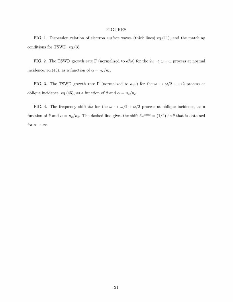
FIGURES

FIG. 1. Dispersion relation of electron surface waves (thick lines) eq.(11), and the matching

conditions for TSWD, eq.(3).

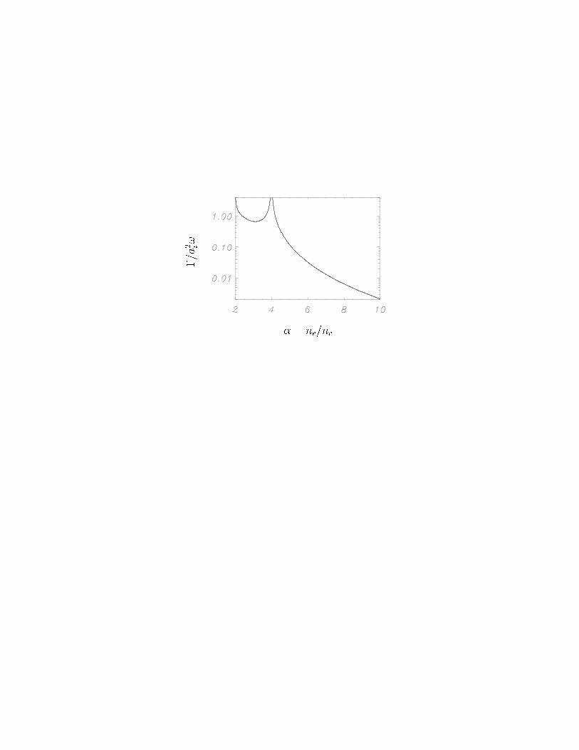
FIG. 2. The TSWD growth rate Γ (normalized to a2iω) for the 2ω → ω + ω process at normal

incidence, eq.(43), as a function of α = ne/nc.

FIG. 3. The TSWD growth rate Γ (normalized to aiω) for the ω → ω/2 + ω/2 process at

oblique incidence, eq.(45), as a function of θ and α = ne/nc.

FIG. 4. The frequency shift δω for the ω → ω/2 + ω/2 process at oblique incidence, as a

function of θ and α = ne/nc. The dashed line gives the shift δωmax = (1/2) sin θ that is obtained

for α → ∞.

21

0

k

s

!

s

(

k

s

)

!

0

=2

!

p

=

p

2

(!

0

; k

0

)

(!

+

; k

+

)

(!

�

; k

�

)

� = n

e

=n

�

=

a

2 i

!

� (degrees)

�

=

a

i

!

arX

iv:p

hysi

cs/0

1050

17v4

[ph

ysic

s.pl

asm

-ph]

26

Apr

200

2

Two-surface wave decay

Andrea Macchi∗, Fulvio Cornolti and Francesco Pegoraro

Dipartimento di Fisica, Universita di Pisa e

Istituto Nazionale Fisica della Materia (INFM), sezione A,

Via Buonarroti 2, I-56100 Pisa, Italy

Abstract

The parametric excitation of pairs of electron surface waves (ESW) in the

interaction of an ultrashort, intense laser pulse with an overdense plasma

is discussed using an analytical model. The plasma has a simple step-like

density profile. The ESWs can be excited either by the electric or by the

magnetic part of the Lorentz force exerted by the laser and, correspondingly,

have frequencies around ω/2 or ω, where ω is the laser frequency.

Typeset using REVTEX

∗E-mail: macchi@df.unipi.it

1

I. INTRODUCTION

Surface wave (SW) excitation has been widely studied in the past as a mechanism for

electromagnetic (EM) wave absorption in highly inhomogeneous plasmas in several regimes

and for different target geometries [1,2] and, more recently, in the specific case of solid

targets irradiated by intense, ultrashort laser pulses [3,4]. The key problem in the linear

mode conversion of the EM wave (the laser pulse) into an SW of the same frequency ω is

that the phase matching between the two waves is not possible at a simple plasma-vacuum

interface. The reason for this is that for an SW vave the wavevector along the plasma surface

ks is larger than ω/c, and thus cannot be equal to the component of the EM wavevector in

the same direction kt = (ω/c) sin θ, where θ is the incidence angle of the laser pulse. Linear

mode conversion of the laser pulse into an SW is possible in specifically tailored density

profiles, e.g. for a “double-step” density profile (i.e. at the interface between an underdense

plasma region where ω > ωp and an overdense region where ω < ωp, with ωp the plasma

frequency), or if a periodic surface modulation with wavevector kp = kt − ks exists, such

that the matching condition for the wavevectors is

kt = ks + kp. (1)

In practical applications, corrugated targets are used to optimize SW generation at a given

incidence angle. Other possible schemes of SW excitation are discussed, e.g., in Refs. [2,3].

In this paper, we discuss a different mechanism of electron surface wave (ESW) excitation

by ultrashort laser pulses, based on the generation of two counterpropagating ESWs. The

basic idea is as follows. An intense laser pulse impinging on an overdense, step-boundary

plasma drives electron oscillations at the frequencies ω and 2ω by the electric and the

magnetic part of the Lorentz force , respectively. The electron response may be viewed as

a superposition of “forced” surface modes with frequency ω0 = ω or 2ω, respectively, and

wavevector k0 = (ω0/c) sin θ. Each of these forced modes may “decay” parametrically into

two ESWs (labeled “+” and “−”, respectively) provided that the matching conditions for a

three-wave process hold:

2

k0 = k+ + k−, (2)

ω0 = ω+ + ω−. (3)

No pre-imposed target modulation is required to satisfy these relations, as depicted in Fig.1.

The ESW frequencies may be written as ω± = ω0/2 ± δω. Thus, the “decay” of the mode

excited by the electric (magnetic) force leads to the generations of ESWs with frequencies

around ω/2 (ω). We call this process “two-surface wave decay” (TSWD) in analogy to the

well-known “two-plasmon decay” parametric instability in laser-plasma interactions.

Earlier investigations of parametric and three-wave nonlinear processes involving ESWs

have been previously carried out in different regimes [5,6]. In particular, the parametric

excitation of pairs of subharmonic ESWs in a magnetized plasma by an external EM wave

was studied in Refs. [7]. These studies were restricted to the electrostatic limit in which

the ESW frequency is ωs ≃ ωp/√2 (see [8] and eq.(11) below) and does not depend on

the wavevector ks in a semi-infinite, step boundary plasma (e.g. with a density profile

ni = niΘ(x), where Θ(x) is the Heaviside step function). In the electrostatic limit the phase

matching with an impinging EM wave is possible only for particular target geometries where

the frequency of electrostatic SWs depends on ks (e.g. a plasma slab of thickness d where ωs

depends on the product ksd [5]). In our model, we assume a semi-infinite geometry but we do

not use the electrostatic approximation, and therefore in general the frequency ωs of ESWs is

significantly lower than ωp/√2 and depends on ks, approaching the EM limit ωs ≃ ksc when

ωs → 0. This allows the matching conditions (3) to be satisfied in a semi-infinite plasma.

It is interesting to notice that in Ref. [9] it has been shown that two counterpropagating

ESWs generate nonlinear radiation at a frequency that is the sum of the ESW frequencies;

this process may be regarded, in some sense, as the inverse process of the TSWD.

One of the main results of this paper is that the intense v × B force at 2ω of the

laser pulse may drive a “2ω → ω + ω” decay with a growth time of a few laser cycles.

In this paper, we focus on this case because of its direct relevance to the interpretation

of recent numerical simulations in two dimensions (2D) for normal laser incidence, which

3

have provided evidence for this process [10]. Note that the surface oscillations observed in

Ref. [10] and theoretically studied in the present paper are different from the grating-like

surface inhomogeneities induced by the magnetic force that were studied in Ref. [11]; these

latter “non-parametric” surface structures oscillate at the same frequency 2ω of the driving

force and are generated at oblique incidence only. In the case of a p-polarized laser pulse at

oblique incidence, we show below that the parametric process may be driven by the electric

force leading to the generation of subharmonic ESWs around the frequency ω/2.

The primary aim of this paper is to describe the “basic principle” of the TSWD as

a possible route to the generation of surface waves and to outline an analytical model

for the TSWD. Therefore, for the sake of simplicity, we use a cold fluid, non-relativistic

plasma model that can be tackled analytically. However, we believe that the TSWD is a

general process that may occur for laser and plasma parameters beyond the limits of the

approximations used in the present paper. Relativistic and kinetic effects, the inclusion

of damping mechanisms and the fully nonlinear evolution of the TSWD are left for future

investigations.

II. THE MODEL

In our model, we consider a cold plasma with immobile ions and a step-like density

profile ni(x) = niΘ(x). The laser pulse has frequency ω, linear polarization and wavevector

k = (ω/c)(x cos θ + y sin θ). Translational invariance along z is assumed. For both s- and

p-polarizations, all fields oscillating at the frequency ω can be determined inside and outside

the plasma from general Fresnel formulae for refraction and transmission at a boundary

[12] between vacuum and a medium with an (imaginary) refractive index n given by n2 =

1− ω2p/ω

2 < 0, ωp = (4πnie2/me)

1/2 being the plasma frequency.

In what follows we study the excitation of “H” ESWs with the magnetic field in the

z direction. Thus, we deal with an effectively 2D geometry, in which B = Bz and the

Maxwell-Euler equations read

4

∇ ·E = 4πe(n0 − ne), (4)

∇×E = −1

c∂tBz, (5)

∇×B =4π

cj+

1

c∂tE, (6)

me∂tv = −mev · ∇v− e(

E+v

c×B

)

(7)

and the current density is given by j = −enev.

We adopt the following expansion for all fields

F (x, y, t) = Fi(x) + ǫF0(x, t− y sin θ/c) + ǫ2[f+(x, y, t) + f−(x, y, t)], (8)

where ǫ is a small expansion parameter and f stands either for the electron density or the

velocity or for the EM fields in the (x, y) plane. In this expansion, Fi represents unperturbed

fields of zero order (e.g., ni). The term F0 represents the “pump” field at the frequency ω0,

that is taken to be of order ǫ and is written as

F0 = F (ω0)(x)eiω0(t−y sin θ/c) + c.c. (9)

In what follows the cases with ω0=ω and ω0 = 2ω are studied separately. The last term in

(8) is the sum of two counterpropagating surface modes, which are assumed to be of order

ǫ2 and are written as

f± =1

2

[

f(ω±)± (x)eik±y−iω±t

]

+ c.c.. (10)

Using expansion (8), the coupling between the pump and the surface modes is of order ǫ3.

Thus, from eqs.(4-5-6-7) we obtain to order ǫ the pump fields. To order ǫ2, we obtain a

set of linearized, homogeneous 2D Maxwell-Euler equations which have ESWs as normal

modes. Note that terms such as v0 · ∇v0 in the Euler equation are also of order ǫ2, but are

non resonant with the ESWs at the frequencies ω±. Such terms represent a source term for

harmonic oscillations at 2ω0 and can be neglected in our model.

ESWs are “H” waves which can propagate in a dielectric medium along a layer of dis-

continuity of the dielectric function, with the latter changing sign across the boundary [13].

5

For a cold, step-boundary plasma there is no volume charge density perturbation associated

with SWs, i.e. ∇ ·E = −4πeδne = 0. At a vacuum-plasma interface, electrons do not enter

the vacuum side, but are “stopped” at the interface (x = 0) forming a surface charge layer.

The dispersion relation for an SW of frequency ωs and wavevector ks is

k2s =

ω2s

c2ω2p − ω2

s

ω2p − 2ω2

s

=ω2s

c2αs − 1

αs − 2. (11)

We have set for convenience αs = ω2p/ω

2s . The dispersion relation (11) is shown in Fig.1.

The EM field envelopes (see eq.(10)) are given by

Esy(x) = Es

y(0)[

Θ(−x)eq<x +Θ(x)e−q>x]

,

Bsz(x) =

iωs/c

q<Es

y(0)[

Θ(−x)eq<x +Θ(x)e−q>x]

,

Esx = ikEs

y(0)

[

Θ(−x)eq<x

q<−Θ(x)

e−q>x

q>

]

, (12)

where q> = (ωs/c)(αs − 1/√αs − 2), q< = (ωs/c)(1/

√αs − 2). The velocity fields are found

from vs = (ie/meωs)Es.

All feedback effects of the nonlinear coupling on the pump fields are neglected. The

coupling terms that lead to the excitation of the ESW with frequency ω± may be represented

by the nonlinear force

f(NL)± = f

(NL)

± (x)eik±y−iω±t = −[

me(v∓ · ∇v0 + v0 · ∇v∓) +e

c(v0 ×B∓ + v×B0)

]

res. (13)

In the term in square brackets on the r.h.s of (13) only “resonant” terms with the same phase

of f(NL)± are included. Obviously, these terms exist if the matching conditions (3) hold.

The nonlinear coupling leads to the parametric excitation and growth of ESWs. We thus

let the ESW envelopes vary slowly in time, i.e.

f±(x) → f±(x, ǫt) (14)

To evaluate the growth rate, we use an energy approach. The surface energy density of the

ESW that will be needed in the calculations is given by

6

U± =k

2π

∫ +π/k

−π/kdy∫ +∞

−∞dx⟨

u(K)± + u

(F )±

⟩

, (15)

where the brackets denote average over one laser cycle and u(K)± and u

(F )± are the volume

densities of the kinetic and EM fields energies, respectively:

u(K)± =

men0

2|v±|2 , (16)

u(F )± =

1

8π

(

|E±|2 + |B±,z|2)

. (17)

The kinetic energy contribution vanishes for x < 0. Using eqs.(12) and v±,x(0+) =

v±,y(0)/√α− 1, and finally summing the two contributions we obtain for the total surface

energy U± = M±|v±,y|2/2 where

M± =menic

4ω±

α±(α± − 2)1/2(α2± − 2α± + 2)

(α± − 1)2. (18)

To obtain an expression for the temporal variation of U± due to the nonlinear coupling

forces, we write the Euler and the Ampere equation for the ESW fields keeping terms up to

order ǫ3 and disregarding terms that are non-resonant with the oscillation:

me∂tv± = −eE± + ǫf(NL)± , (19)

∇×B± =4π

c

(

−enov± + ǫJ(NL)±

)

+1

c∂tE±, (20)

where f(NL)± is given by eq.(13), and J

(NL)± = −eδn(ω0)

e v±. Using eqs.(19-20) together with

Maxwell’s equations we obtain for the temporal variation of the energy densities

∂tu(K)± = −enov± · E± + ǫf

(NL)± · v±, (21)

∂tu(F )± = −∇ · S± − ǫJ

(NL)± · E±, (22)

where S± = (c/4π)E± × B± is the Poynting vector of the ESW. We integrate the sum of

the energy densities over space and average over time. Noting that the total flux of S±

vanishes because of the evanescence of the ESW fields, we finally obtain the equation for

the evolution of the total energy U of the ESW:

7

∂tU± =k

2π

∫ +π/k

−π/kdy∫ +∞

0dx∂t

⟨

men0

2|v±|2 +

1

8π

(

|E±|2 + |B±|2)

⟩

= ǫk

2π

∫ +∞

0dx∫ +π/k

−π/kdy⟨

v± ·(

eδn(ω0)e E± + fNL

±

)⟩

. (23)

The integral extends for x > 0 only since there are no electrons for x < 0.

From eq.(23), performing the integral and neglecting high order terms one obtains two

coupled equations in the general form

M±

2∂t|v±|2 = A0ω|v+||v+|S± sinϕ, (24)

where A0 is the amplitude of the pump mode in dimensionless units, S± are positive factors

depending on ωp/ω and θ, and ϕ is obtained from the phase factors of the pump and ESW

modes as ϕ = φ+ + φ− − φ0. From (24) one easily obtains

∂2t |v±| = (A0ω)

2

(

S+S−

M+M−

)

sin2 ϕ|v±|. (25)

Setting sinϕ = 1 simply corresponds to finding the relative phase of the growing modes with

respect to the phase of the pump mode. The growth rate of ESWs is then

Γ = A0ω

√

S+S−

M+M−

. (26)

In the next section we use the analytical method outlined above to study TSWD in two

cases of particular relevance: TSWD driven by the v × B force for normal laser incidence

(which we name “2ω → ω + ω” decay), and TSWD driven by the electric force for oblique

laser incidence and p-polarization (“ω → ω/2 + ω/2” decay).

III. “2ω → ω + ω” DECAY

To discuss the “2ω → ω + ω” decay, we restrict ourselves for simplicity to the case of

normal incidence, as was done in the simulations reported in Ref. [10]. Thus, the ESW

frequency ω± = ω and k+ = −k− The case of oblique incidence is indeed very similar, the

main difference being that the matching condition k+ + k− = (2ω/c) sin θ holds, causing a

8

shift δω 6= 0 between the two ESWs. It is found that the growth rate decreases monotonically

with increasing incidence angle, since the pump force has a maximum at normal incidence

[14].

The laser wave can be represented by a single component of the vector potential, Az =

Az(x, t), that for x > 0 is given by

Az(x, t) = Az(x) cosωt = Az(0)e−x/ls cosωt, (27)

where ls = c/(ω2p − ω2)1/2 is the screening length. Imposing boundary conditions for the

incident and reflected waves one finds Az(0) = 2Ai(ωls/c)(1 + ω2l2s/c2)−1/2, where Ai is the

amplitude of the incident field.

Electrons perform their quiver motion in the z direction. Thus, the magnetic force term

is in the x direction and has a secular term (0ω), named the ponderomotive force, and an

oscillating term (2ω) that, in what follows, we simply name the v × B force. The secular

term corresponds to radiation pressure and creates a surface polarization of the plasma.

The v × B force drives a longitudinal, electrostatic oscillation that acts as a pump mode

for TSWD. In the expansion (8), the pump amplitude is supposed to be of order ǫ. As will

be shown below, coupling between 1D and 2D fields occurs only in the overdense plasma

(x > 0). Thus, since the v × B force is quadratic in the laser field, the expansion (8)

also implies a(0) ∼ ǫ1/2, where a(0) is the (dimensionless) laser amplitude at the surface

of the plasma, e.g a(0) = (eAz(0)/mc2). For overdense plasmas a(0) ∼ (ω/ωp)ai < ai,

where ai = (eAi/mc2). This yields ǫ ∼ (ω/ωp)2 a2i = (nc/ne) a

2i , where nc = meω

2/4πe

is the “critical” density. We therefore expect our expansion procedure to be valid even at

relativistic fields amplitudes ai ≥ 1 for high enough plasma densities.

We now derive the solutions for the 1D pump fields at 2ω. The electron oscillation

velocity is obtained from the conservation of canonical momentum as mevz = eAz/c. For

normal laser incidence, the longitudinal v×B force is given by

− e

cvzBy = − e2

mec2Az∂xAz ≡ F 0(x)(1 + cos 2ωt), (28)

9

where we have set F 0(x) = (mec2/2ls)a

2se

−2x/ls ≡ F 0e−2x/ls . To order ǫ, one obtains the

following equations for the longitudinal, electrostatic motion :

me∂tV(2ω)x = −e(E(0)

x + E(2ω)x ) + F 0(x)(1 + cos 2ωt), (29)

∂x(E(0)x + E(2ω)

x ) = −4πe(δn(0)e + δn(2ω)

e ), (30)

∂tδn(2ω)e = −n0∂xV

(2ω)x . (31)

All fields in the equations above decay inside the plasma as exp(−2x/ls). The secular part

simply gives eE(0)x (x) = F 0(x) and δn(0)

e = −∂xF0(x)/4πe2 = F 0(x)/2πe2ls. For the motion

at 2ω one obtains

V (2ω)x =

−iF 0

ωmeD

(

ω2

ω2p

)

e−2x/ls, (32)

δn(2ω)e = ni

F 0

ω2plsmeD

e−2x/ls , (33)

eE(2ω)x =

F 0

2De−2x/ls . (34)

The denominator D is given by

D = 1− 4ω2

ω2p

= 1− 4nc

ne

, (35)

which shows the well-known resonance at ne = 4nc due to excitation of plasmons with

frequency ωp = 2ω by the v×B force.

The difference between the total number of electrons and ions for x > 0 is, to order ǫ,

∆N (x>0)e =

∫ +∞

0dx(

δn(2ω)e + δn(0)

e

)

=F 0

2πe2

(

1 +cos 2ωt

D

)

. (36)

The fact that ∆N (x>0)e > 0 during most of the oscillation implies that, due to compression

from the ponderomotive and v × B forces, electrons leave behind a charge depletion layer

of thickness ζ = ∆N (x>0)e /ni. We note that ζ is of order ǫ, thus to lowest order it is correct

to treat the charge depletion layer as a surface layer. Heuristically, the oscillating behavior

of ζ describes the plasma “moving mirror” effect [15]: due to charge depletion the laser

is reflected at x = ζ rather than exactly at x = 0. This leads to the appearance of high

harmonics in the reflected light.

10

Since |D| < 1, there is always a time interval in which electrons are pulled into vacuum

forming a cloud of negative charge. This interval is very short for ne/nc ≫ 4, i.e. D ≃ 1,

but for lower densities it is relevant in the interaction process. The motion in vacuum

is strongly anharmonic and more difficult to solve analitically than the motion inside the

plasma. However, it is found in section III that the surface modes gain energy during the

phase of electron motion inside the plasma only, so that the expressions of fields for x < 0

are not needed. Nevertheless, we have to assume that the density of the electron cloud for

x < 0 is low enough for the laser propagation not to be affected.

Using eq.(32), the NL force (13) may be written in terms of the oscillation velocity V (2ω)x

as follows:

fNL± = −

[

me

(

V (2ω)x (x)∂xv∓ + vx,∓∂xV

(2ω)x (x)x

)

− e

cV (2ω)x (x)Bz,∓y

]

. (37)

Because of the symmetry with respect to inversion of the y axis, the two ESWs may

differ only by a phase factor and have the same amplitude and energy. Inserting the force

(37) in the energy equation (23) and performing the integral in y we obtain for the ESW

energy U = U±

∂tU =1

8

∑

l=+k,−k

∫ +∞

0dxv∗

+l ·(

eδne(2ω)(x)E

∗

−l −men0v∗x,−l∂xV

(2ω)x (x)

−men0V(2ω)x (x)∂xv

∗−l + n0

e

cV (2ω)x (x)B∗

z,−ly ) + c.c. (38)

We rewrite all fields as functions of V (2ω)x and v±. We obtain, after some algebra

∂tU =meni

2(1 + q>ls)ℜ{

V (2ω)x

[

(1 + q>ls)v∗+v

∗− + 2v∗x,+v

∗x,− − v∗y,+v

∗y,−

q>ls

]

,

}

. (39)

All the terms of eq.(39) are proportional to

ℜ(

V (2ω)x v∗+v

∗−

)

=∣

∣

∣V (2ω)x v2±

∣

∣

∣ cos(φ+ π/2), (40)

where φ = φ+ +φ−, φ± being the phase angles of v±, and we used eq.(32) and the fact that

F 0 is real and positive. Thus, the phase of the growing ESWs with respect to the v×B force

11

is such that φ = −π/2, the value for which the growth rate is positive and has a maximum.

The overlap of the two ESWs gives

v+2eiky−iωt +

v−2e−iky−iωt =

|v±|2

e−iωt(

eiky+iφ+ + e−iky+iφ−

)

= |v±|e−iωt−iπ/4 cos (ky +∆φ) , (41)

where ∆φ = (φ+ − φ−)/2. This is a standing wave which has a temporal phase shift −π/4

with respect to the v×B force of eq.(28). The phase is such that, at a given position in y,

the temporal maxima of V (2ω)x and v(ω) overlap once for laser cycle. The angle ∆φ gives the

location of the maxima of the standing wave on the y axis, which depends on the arbitrary

choice of the initial phase.

Using eq.(40), we can rewrite the energy variation as

∂tU = meni|V (2ω)x |

[

|v+|2 +2|vx,k|21 + q>ls

− 2|vy,k|2q>ls(1 + q>ls)

]

. (42)

Note that ∂tU > 0 since q>ls =√

(α− 1)(α− 2)−1 > 1, where α = ω2p/ω

2 = ne/nc.

Eliminating V (2ω)x as a function of ai and α, after some algebra the growth rate Γ is obtained:

Γ = 4ωa2i(α− 1)3/2

α|α− 4|[(α− 1)2 + 1](α− 2)1/2

[

1 +2

α(1 + q>ls)− 2(α− 1)

αq>ls(1 + q>ls)

]

≃ 4ωa2i(α− 1)3/2

α|α− 4|[(α− 1)2 + 1](α− 2)1/2. (43)

The leading contribution was highlighted in the last equality.

A plot of the growth rate as a function of α is given in Fig.2. For moderately overdense

plasmas, Γ is a considerable fraction of the laser frequency. The resonance at ne = 4nc

is due to the resonant behavior of the pump field. The growth rate diverges also in the

electrostatic limit when ne → 2nc. However, in this limit the value of k tends to infinity,

i.e. the wavelength becomes very small and one expects that this second resonance might

be damped by thermal effects, which are neglected in our model and are left for future

inevstigations.

The comparison of spatial and temporal scales predicted from this model with the sim-

ulation results shows reasonable agreement for laser and plasma parameters such that our

12

expansion procedure is valid [10]. We note that simulation results for high intensities in the

relativistic regime suggest that a 2ω → ω + ω TSWD-like process still occurs and produces

strong rippling of the plasma surface; the spatial scales are different from those predicted

by our analytical, cold fluid model, but still of the same order of magnitude.

We conclude this section by noting that, although we took the laser polarization along

z, the whole derivation is valid at normal incidence for any polarization direction. The only

difference in 2D geometry is that, for the laser polarization along y, the quiver oscillations

at ω and the ESW oscillations at the same frequency overlap. This is observed in numerical

simulations [14].

IV. “ω → ω/2 + ω/2” DECAY

A case of particular interest is that of oblique incidence and p-polarization of the laser

pulse, since these conditions lead in general to a stronger plasma coupling. In the preceding

section we have found that the 2ω → ω+ω decay is driven by the longitudinal component of

the velocity field, as shown by eq.(37). For p-polarization and θ 6= 0 the electric field drives a

strong longitudinal oscillation at the frequency ω; thus, one expects that the TSWD process

leads to the generation of subharmonic ESWs, having frequencies around ω/2, with peak

efficiency at some angle of incidence. As shown below, this picture is substantially correct.

However, there is a small but non-vanishing growth rate for the ω → ω/2+ω/2 process even

at normal incidence. In fact, the pump force (13) is now given by

f(NL)± = −me(v∓,x∂xV

(ω) + V (ω)x ∂xv∓)−me(v∓,y∂yV

(ω) + V (ω)y ∂yv∓)

−e

c(V(ω) ×B∓ + v∓ ×B(ω)), (44)

and does not vanish for θ = 0.

The case of oblique incidence and p-polarization of the laser pulse may be tackled with

an approach analogous to that of section III. The main physical difference with the previous

case is that now the “pump” is a divergence-free velocity field at the laser frequency ω, and

13

its amplitude is now proportional to the laser field rather than to the laser intensity. In

applying the expansion procedure (8) again, now ǫ ∼ (ω/ωp)ai (appendix A). Thus, the

limits of validity of this expansion are more restrictive in the present case: the expansion

tends to be valid only for rather high densities or rather low fields. One must also note

that temperature effects, neglected in the cold plasma approximation, are important for low

fields.

The calculation of the growth rate for subharmonic ESWs can be performed by the same

method as in the preceding sections in a straightforward way. The details are reported in

appendix A. As a final result, the growth rate Γ = Γ(α, θ) may be written as

Γ = aiω|FB|(

nc

ne

)5/2

K(α, θ), (45)

where FB is the Fresnel factor for the magnetic field and the factor K(α, θ) scales weakly

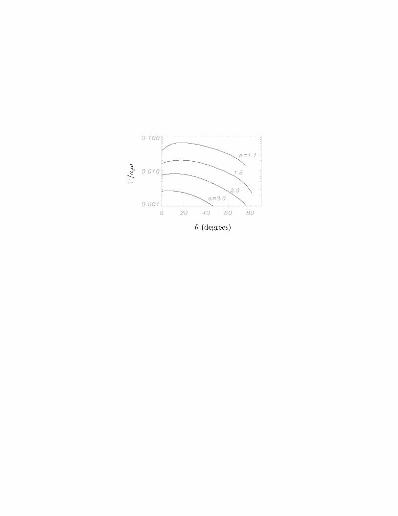
with density. A plot of Γ as a function of θ for different values of α is reported in Fig.3.

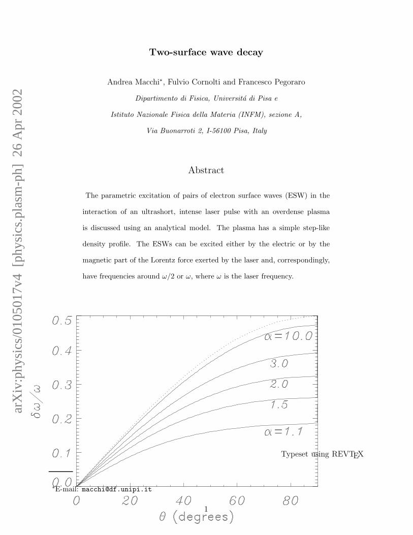
The frequency shift δω of the two ESWs can be calculated as a function of θ and α from

the matching condition k++k− = (ω/c) sin θ. The result is shown in Fig.4. Comparing with

Fig.3, one finds that δω ≈ 0.1ω in conditions favorable to the ω → ω/2 + ω/2 TSWD.

V. DISCUSSION

The TSWD concept has been investigated analytically in two cases that clarify its basic

features in the context of the cold fluid plasma approximation. This process may lead to the

excitation of ESWs by an ultrashort laser pulse in a solid target without any special (e.g.,

grating-like) structure, and even for normal incidence and s-polarization.

In both the cases discussed in this paper, we found a strong decrease of the TSWD growth

rate for increasing densities. This does not necessarily imply that TSWD is not relevant to

short pulse interaction with solid targets which have ne/nc ≫ 1. In fact, important processes

such as high harmonic generation or fast electron production are more efficient when the laser

pulse interacts with a moderate density plasma. This is the case for most of the experiments

14

of short pulse interaction with solid targets, since a moderate density “shelf” is usually

produced at the time of peak pulse intensity by target ablation and plasma hydrodynamic

expansion during the leading edge of the short pulse or during the long prepulse. For

instance, the “2ω → ω+ω” decay appears to be very efficient exactly in conditions favorable

for high harmonics production via the “moving mirror” effect [15,16]. Simulations [10]

suggest that TSWD in strongly nonlinear and relativistic regimes (beyond the limits of the

analytical approach of this paper) may produce surface perturbations acting as a ”seed” for,

e. g. , electron instabilities leading to current filamentation [17,18] or detrimental distortions

of the moving mirrors, and for Rayleigh-Taylor-like (RT) hydrodynamic instabilities occuring

on the time scale of ion motion. In Ref. [10] it is estimated that the growth rate of the RT

instability is much slower than that of TSWD. A different hydrodynamic instability with a

surprisingly high growth rate has been reported in Ref. [19]).

The 2ω → ω+ω and the ω → ω/2+ω/2 processes have been considered independently.

This is appropriate since these are resonant processes which do not interfere with each other.

In principle, both decays may occur during the interaction of an intense laser pulse with

an overdense plasma. According to our analysis the 2ω → ω + ω process appears to have

a stronger growth rate. However, in the case of the ω → ω/2 + ω/2 process our analytical

approach is valid for a very narrow range of parameters only. Either an extension of the

present analytical approach or numerical simulations are needed to investigate the TSWD

for a very intense, p-polarized laser pulse at oblique incidence.

VI. CONCLUSIONS

We have discussed the Two-Surface Wave Decay as a novel mechanism for the excitation

of electron surface waves in the interaction of ultrashort, intense laser pulses with overdense

plasmas. TSWD is based on the parametric excitation of a pair of ESWs. The “pump” force

may either be the magnetic or the electric force of the laser pulse, and leads respectively

to the generation of two ESWs with frequencies close to the laser frequency of half of it.

15

An analytical model for TSWD in the cold fluid plasma, non-relativistic approximation has

been developed. The model supports the interpretation of recent simulation results [10] and

suggests that TSWD may be of relevance in certain regimes of laser interaction with solid

targets.

ACKNOWLEDGMENTS

This work was partly supported by INFM trhough a PAIS project. We are grateful to

Prof. L. Stenflo for bringing many references to our attention and to M. Battaglini for very

useful discussions.

APPENDIX A: GROWTH RATE OF THE ω → ω/2 + ω/2 DECAY

We now give the detailed derivation of the growth rate for the ω → ω/2+ω/2 TSWD of

section IV. The pump fields are easily found with the help of Fresnel formulae and Maxwell

equations. For instance, the magnetic field is given by

B(ω)z (x, t) = B(ω)

z (0+)eiky sin θ−x/lp−iωt + c.c. , (A1)

where the screening length is given by

lp =c

ωp

(

1− ω2

ω2p

cos2 θ

)−1/2

=c

ω

1√α− cos2 θ

, (A2)

and the magnetic field at the surface is given by the Fresnel formula

Bz(0+)

Bz,i=

2n2 cos θ√n2 − sin2 θ + n2 cos θ

=2(α− 1) cos θ

(α− 1) cos θ − i√α− cos2 θ

≡ FB(θ), (A3)

where Bz,i is the incident field amplitude in vacuum. The electric field components are found

by using ∇ · E(ω) = 0 and ∇× E(ω) = i(ω/c)B(ω)z + c.c..

The nonlinear force is given by eq.(37). Evaluating the spatial derivatives as ∂xV(ω) =

−V(ω)/lp, ∂yV(ω) = iktV, ∂yv± = ik±v±, and ∂xv± = −q±v± where q± ≡ q>(ω±), and

keeping resonant terms only we find

16

f(NL)±,x =

me

4

[(

1

lp+ q∓

)

V (ω)x v∗∓,x −

e

mec

(

V (ω)y B∗

∓,z + B(ω)z v∗∓,y

)

−iktV(ω)x v∗∓,y + ik∓V

(ω)y v∗∓,x

]

e−(q∓+1/lp)x + c.c., (A4)

f(NL)±,y =

me

4

[

1

lpV (ω)y v∗∓,x + q∓V

(ω)x v∗∓,y +

e

mec

(

V (ω)x B∗

∓,z + B(ω)z v∗∓,x

)

−i(kt − k∓)V(ω)y v∗∓,y

]

e−(q∓+1/lp)x + c.c.. (A5)

We rewrite all “pump” terms as a function of V (ω)y by using V (ω)

x = iktlpV(ω)y , B(ω)

z =

(mec/elp)(k2t l

2p − 1)V (ω)

y . In a second step we rewrite all SW fields as a function of v±,y by

using v±,x = (ik±/q±)v±,y and b±,z = −meω2±(α± − 1)v±,y/(ecq±). We thus obtain

f(NL)±,x =

me

4V (ω)y v∗∓,y

[

k∓q∓

(kt + ktq∓lp + k∓) +ω2∓

q∓c2(α∓ − 1) +

1

lp

]

e−(q∓+1/lp)x (A6)

≡ me

4V (ω)y v∗∓,yQ±,xe

−(q∓+1/lp)x (A7)

f(NL)±,y =

me

4V (ω)y v∗∓,yi

[

ktlp

(

q∓ − 1

lp− ktk∓

q∓− ω2

∓

q∓c2(α∓ − 1)

)

+ k∓

]

e−(q∓+1/lp)x (A8)

≡ me

4V (ω)y v∗∓,yiQ±,ye

−(q∓+1/lp)x. (A9)

The relations ω2±(α±−1)/q± = ω±c

√α± − 2, k±/q± = 1/

√α± − 1, ktlp = sin θ(α−cos2 θ)−1/2

may be used to simplify the expressions for Q±,x and Q±,y. We thus obtain

Q±,x =1√

α∓ − 1[kt(1 + q∓lp) + k∓] +

ω∓

c

√

α∓ − 2 +1

lp, (A10)

Q±,y = ktlp

(

q∓ − 1

lp− kt√

α∓ − 1− ω∓

c

√

α∓ − 2

)

+ k∓. (A11)

In the energy equation (23), since δn(ω) = 0 the integrand, eliminating v±,x, is given by

⟨

v± · fNL±

⟩

=me

16iV (ω)

y v∗∓,yv∗±,y

(

k±q±

Q±,x +Q±,y

)

+ c.c. (A12)

=me

8ℜ[

iV (ω)y v∗∓,y v

∗±,y

]

(

k±q±

Q±,x +Q±,y

)

. (A13)

We thus find

∂tU± = nime

8

lp1 + (q+ + q−)lp

(

k±q±

Q±,x +Q±,y

)

∣

∣

∣V (ω)y v∓,yv±,y

∣

∣

∣ sinϕ. (A14)

Here, ϕ = (φ++φ−−Φ), where Φ and φ± are the phase factors of V (ω)y and v±,y, respectively.

It is worth rewriting these equations in a more compact form. Introducing ai = eBi/meωc

and using Fresnel’s formulas to eliminate Vy we obtain

17

∂tU± = nime

8aic|FB(θ)||v+,y||v−,y| sinϕG±(α, θ), (A15)

where we have posed G±(α, θ) = G0(α, θ)g±(α, θ) and

G0 =

√α− cos2 θ

(α− 1)[1 + (q+ + q−)lp], (A16)

g± = lp

(

k±q±

Q±,x +Q±,y

)

=1

√

(α+ − 1)(α− − 1)[ktlp(1 + q∓lp) + k∓lp] +

ω∓lpc

√α∓ − 2√α± − 1

+1√

α± − 1

+ktlp

(

q∓lp − 1− ktlp√α∓ − 1

− ω∓lpc

√

α∓ − 2

)

+ k∓lp. (A17)

Using the equations above we obtain the following coupled equations in the form (24) for

the field amplitudes

µ±∂t|v±,y|2 = aiω|v+y||v−y||FB|G± sinϕ, (A18)

where µ± ≡ 4M±/(menic). Thus, the growing modes have relative phases such that sinϕ =

1. The growth rate is given by

Γ = aiω|FB|G0

√

√

√

√

|g+g−|µ+µ−

≡ aiω|FB|(

nc

ne

)5/2

K(α, θ) (A19)

which is the formula (45). A plot of Γ is depicted in Fig.3.

18

REFERENCES

[1] J. M. Kindel, K. Lee, and E. L. Lindman, Phys. Rev. Lett. 34, 134 (1975); T. A.

Davydova, Sov. J. Plasma Phys. 7, 507 (1981).

[2] R. Dragila and S. Vukovic, Phys. Rev. Lett. 61, 2759 (1988); R. Dragila and S. Vukovic,

J. Opt. Soc. Am. B 5, 789 (1988).

[3] R. Dragila and E. G. Gamaly, Phys. Rev. A 44, 6828 (1991); J. Kupersztych and M.

Raynaud, Phys. Rev. E 59, 4559 (1999).

[4] E. G. Gamaly, Phys. Rev. E 48, 516 (1993); S. A. Magnitskii, V. T. Platonenko, and

A. V. Tarasishin, AIP Conf. Proc. 426, 73 (1998).

[5] Yu. M. Aliev, O. M. Gradov and A. Yu. Kirii, Sov. Phys. JETP 36, 663 (1973).

[6] O. M. Gradov and L. Stenflo, Phys. Scripta 29, 73 (1984); L. Stenflo, Phys. Scripta

T63, 59 (1996).

[7] O. M. Gradov and L. Stenflo, Plasma Phys. 22, 727 (1980); O. M. Gradov and L. Stenflo,

Phys. Lett. 83A, 257 (1981); O. M. Gradov, R. R. Ramazashvili and L. Stenflo, Plasma

Phys. 24, 1101 (1982).

[8] P. K. Kaw and J. B. McBride, Phys. Fluids 13, 1784 (1973).

[9] O. M. Gradov and L. Stenflo, Phys. Scripta T63, 297 (1996).

[10] A. Macchi, F. Cornolti, F. Pegoraro, T. V. Liseikina, H. Ruhl, and V. A. Vshivkov,

Phys. Rev. Lett. 87, 205004 (2001).

[11] L. Plaja, L. Roso, and E. Conejero-Jarque, Laser Phys. 9, 1 (1999); L. Plaja, E.

Conejero-Jarque, and L. Roso, Astrophys. J. Supp. Ser. 127, 445 (2000).

[12] J. D. Jackson, Classical Electrodynamics, 2nd Edition (John Wiley and Sons, Inc., 1975),

par.7.3.

19

[13] L. D. Landau, E. M. Lifshitz, and L. P. Pitaevskij, Electrodynamics of Continuous Media

(Pergamon Press, New York, 1984), p.306.

[14] A. Macchi, M. Battaglini, F. Cornolti, F. Pegoraro, T. V. Liseikina, H. Ruhl, and V.

A. Vshivkov, “Parametric generation of surface deformations in laser interaction with

overdense plasmas”, to be published in Las. Part. Beams (2002).

[15] S. V. Bulanov, N. M. Naumova and F. Pegoraro, Phys. Plasmas 1, 745 (1994).

[16] P. Gibbon, Phys. Rev. Lett. 76, 50 (1996). R. Lichters, J. Meyer-ter-Vehn, and A.

Pukhov, Phys. Plasmas 3, 3425 (1996).

[17] F. Califano, R. Prandi, F. Pegoraro, and S. V. Bulanov, Phys. Rev. E 58 7837 (1998).

[18] B. Lasinski, A. B. Langdon, S. P. Hatchett, M. H. Key, and M. Tabak, Phys. Plasmas

6, 2041 (1999); Y. Sentoku, K. Mima, S. Kojima, and H. Ruhl, Phys. Plasmas 7, 689

(2000).

[19] E. G. Gamaly, Phys. Rev. E 48, 2924 (1993).

20

FIGURES

FIG. 1. Dispersion relation of electron surface waves (thick lines) eq.(11), and the matching

conditions for TSWD, eq.(3).

FIG. 2. The TSWD growth rate Γ (normalized to a2iω) for the 2ω → ω + ω process at normal

incidence, eq.(43), as a function of α = ne/nc.

FIG. 3. The TSWD growth rate Γ (normalized to aiω) for the ω → ω/2 + ω/2 process at

oblique incidence, eq.(45), as a function of θ and α = ne/nc.

FIG. 4. The frequency shift δω for the ω → ω/2 + ω/2 process at oblique incidence, as a

function of θ and α = ne/nc. The dashed line gives the shift δωmax = (1/2) sin θ that is obtained

for α → ∞.

21