Anderson localization in a multi-particle continuous model with … · Anderson localization in a multi-particle continuous model with an alloy-type external potential A. Boutet de

Anderson localization in a multi-particle

continuous model with an alloy-type external

potential

A. Boutet de Monvel1, V. Chulaevsky2, P. Stollmann3, Y. Suhov4

1Institut de Mathematiques de JussieuUniversite Paris 7175 rue du Chevaleret, 75013 Paris, FranceE-mail: [email protected]

2Departement de MathematiquesUniversite de Reims, Moulin de la Housse, B.P. 1039,51687 Reims Cedex 2, FranceE-mail: [email protected]

3 Fakultat fur MathematikTechnische Universitat Chemnitz09107 Chemnitz, GermanyE-mail: [email protected]

4 Statistical Laboratory, DPMMS

University of Cambridge, Wilberforce Road,

Cambidge CB3 0WB, UK

E-mail: [email protected]

Abstract: We establish the exponential localization in a multi-particle Ander-son model in a Euclidean space R

d, d ≥ 1, in presence of a non-trivial short-range interaction and a random external potential of an alloy type. Specifically,we prove all eigenfunctions with eigenvalues near the lower edge of the spectrumdecay exponentially in L2-norm.

1. Introduction. The N-particle Hamiltonian in the continuum

1A. The model. This paper considers an N -particle Anderson model inRd with interaction. The Hamiltonian H

(= H(N)(ω)

)is a random Schrodinger

operator of the form

H = −1

2∆ + U(x) + V(ω;x) (1.1)

acting in L2(Rd×. . .×Rd) ≃ L2(R

d)⊗N . This means that we considerN quantumparticles, each living in Rd, in the following fashion. The joint position vector is

x = (x1, . . . , xN ) ∈ Rd × . . . × R

d, where component xj =(x(1)j , . . . , x

(d)j

)∈ R

d

represents the coordinates of the j’s particle, j = 1, . . . , N . Next,

−1

2∆ = −

1

2

∑

1≤j≤N

∆j

is the standard kinetic energy operator obtained by adding up the kinetic energies

−1

2∆j of individual particles and assuming that the particles are of identical

2 A. Boutet de Monvel1, V. Chulaevsky2, P. Stollmann3, Y. Suhov4

masses. In the case of different masses, −1

2∆ would have been replaced by the

sum −1

2

∑

1≤j≤N

1

mj∆j , without changing the analysis involved. As usually, ∆j

stands for the Laplaciand∑

i=1

∂2

∂x(i)j

2 in Rd.

The interaction energy operator is denoted by U(x): it is the operator ofmultiplication by a function x ∈ Rd×. . .×Rd 7→ U(x), the inter-particle potential(which can also incorporate a deterministic external potential). Finally, the termV(ω;x) represents the operator of multiplication by a function

x 7→ V (ω;x1) + . . .+ V (ω;xN ), x = (x1, . . . , xN ) ∈ Rd × . . .× R

d, (1.2)

where x ∈ Rd 7→ V (x;ω), x ∈ Rd, is the random external field potential. As-sumptions on U(x) and V (ω;x) are discussed below; in essence, U is required tobe a sum of short-range inter-particle potentials while V is assumed to be of analloy type.

We will analyse spectral properties of operator H by using the so-called Multi-Scale Analysis (MSA) method, more precisely, its ‘continuous-space’ version. Ourgoal here is two-fold.

• First, we show that of the continuous-space version of the MSA can be re-duced, in a certain way, to its discrete counterpart, for an auxiliary lattice prob-lem, and the corresponding argument works equally well for systems with severalparticles. The MSA is known to be a powerful and versatile method successfullyapplied to a number of spectral problems in random media. It was originally de-veloped for a single-particle lattice (tight-binding) Anderson models (cf. [FS83,FMSS85], [DK89]) and later adapted to problems in a Euclidean space. See[BCH97,CH94,DS01,HM84,KSS98A,KSS98B,K95]; the monograph [St01] con-tains more complete references up to the year 2000. Notable later developments,still for one-particle systems, are [GK01], [BK05] (solving the notorious problemof localization for a Bernoulli–Anderson model in Rd), and [AGKW08], wherethe MSA was adapted to a large class of singular distributions of the externalrandom potential.

However, the existing continuous adaptations are technically more involvedthan the original lattice version of the MSA. This leads to greater complexity ofthe continuous localization analysis, particularly when one attempts to treat thecase of more than one particle. In contrast, the reduction to an auxiliary latticeproblem presented in this paper works in a fairly general fashion. This reductionis encapsulated in the so-called Geometric Resolvent Inequalities (GRI) andallows a direct application of lattice techniques (and some additional generalfacts) in a ready-made form which is technically much less involved.

In addition, we simplify an important ingredient of the many-particle latticeMSA, following the strategy outlined in [C08]. As a result, a relatively straight-forward strategy of the proof of Anderson localization emerges, applicable forboth discrete and continuous multi-particle models.

• Second, we combine in this paper the above-mentgioned reduction techniqueswith the method from [CS09A] (and in part from [CS09B]), where a multi-particle tight-binding Anderson localization has been proved, for large disorders.As a result, we prove here Anderson localization near the lower edge of the

Title Suppressed Due to Excessive Length 3

spectrum for an N -particle model in a Euclidean space Rd, d ≥ 1, with an alloy-type external random potential and a short-range interaction between particles.See Theorem 1.1 below. An essential ingredient here are the so-called Wegner-type bounds obtained for alloy-type systems in [BCSS08A], [BCSS08B].

1B. Basic concepts. Throughout this paper, we work with cubes with theedges parallel to the co-ordinate axes in the Euclidean spaces Rd·n := Rd × . . .×Rd (n times) representing the n-particle configuration space, n = 1, . . . , N :

ΛL(u) = ×1≤i≤d

[u(i) − L, u(i) + L

], and ΛL(u) = ×

1≤j≤nΛL(uj), (1.3)

where u =(u(1), . . . ,u(d)

)∈ Rd(= Rd·1) and u = (u1, . . . , un) ∈ Rd·n. For our

purpose, it suffices to consider only cubes centered at lattice points u ∈ Zd andu ∈ Zd·n := Zd × . . . × Zd. With few exceptions, boldface symbols indicate n-particle objects, related to Rd·n or Zd·nd; a notable exceptions is the symbol1A standing for an indicator function of a set A ⊂ Rd·n and – with a slightabuse of notation – for the operator of multiplication by this function. It istechnically convenient to use the max-norm for vectors x =

(x(1), . . . , x(d)

)∈ R

d

and x = (x1, . . . , xn) ∈ Rd·n:

|x| = max1≤i≤d

|xi|, |x| = max[|x1|, . . . , |xn|

]. (1.4)

Correspondingly, the distance dist figuring in the sequel refers to to this norm.In terms of the max-norm a cube ΛL(u) coincides with the ball in Rd of radiusL about point u and ΛL(u) gives the ball in Rd·n of radius L about point u.

We will also need lattice cubes:

BL(u) = ΛL(u) ∩ Zd, and BL(u) = ΛL(u) ∩ Z

d·n. (1.5)

and unit cells (or simply cells):

C(u) = Λ1(u) ⊂ Rd, and C(u) = Λ1(u) ⊂ R

d·n. (1.6)

In what follows, all these sets are also often called boxes, single-particle forΛL(u), BL(u) and C(u) and n-particle for ΛL(u), BL(u) and C(u). A union ofcells is referrred to as a cellular set.

1C. Interaction and external field potentials. The interaction potential Uin Eqn (1.1) is assumed to be of the form

U(x) =∑

k=1,...,N

∑

1≤i1<...<ik≤N

Φ(k)(xi1 , . . . , xik), x = (x1, . . . , xN ) ∈ R

d·N ,

(1.7)where function Φ(k) : Rd·k → R, 1 ≤ k ≤ N , represents a k-body interactionpotential and satisfies the following property:

(I) Upper-boundedness, non-negativity, symmetry and finite range:

∀ k = 1, . . . , N : 0 ≤ Φ(k)(y) ≤ u0, y = (y1, . . . , yk) ∈ Rd·k,∀ k = 2, . . . , N : Φ(k)(y1, . . . , yk) = Φ(k)(yσ(1), . . . , yσ(k)),

∀ permutation σ on 1, . . . , k,

∀ k = 2, . . . , N : Φ(k)(y) = 0 when max1≤i≤N

(minj 6=i

[|yi − yj |

])≥ r0,

(1.8)


where constants u0, r0 ∈ (0,+∞).

Remark 1.1. Non-negativity of potentials Φ(k) is used to simplify the state-ment of the main result (see Theorem 1.1 below) and shorten the proof oftechnical assertions. We can also relax the boundedness condition, by allow-ing hard-core potentials where, ∀ k ≥ 2, Φ(k)(y1, . . . , yk) = +∞ whenever

min1≤i<j≤k

∣∣yi − yj

∣∣ < r1 where r1 ∈ (0, r0). On the other hand, the finite-range

condition is essential for the method used, and extending our Theorem 1.1 tothe case of infinite-range potentials seems a challenging problem.

Further, the random external potential V (x;ω), x ∈ Rd, ω ∈ Ω, is assumedto be of alloy-type, over a cubic lattice:

V (x;ω) =∑

s∈Zd

Vs(ω)ϕs(x − s). (1.9)

Here V = (Vs, s ∈ Zd), is a family of real random variables Vs on some prob-

ability space (Ω,B,P) and ϕs, s ∈ Zd is a (nonrandom) collection of ‘bump’functions y ∈ Rd 7→ ϕs(y). In probabilistic terms, V is a real-valued randomfield (RF) on Zd. Physically speaking, the random variable Vs represents theamplitude of ‘impurity’ at site s of lattice Zd while the function ϕs describes the‘propagation’ of the impact of this impurity across Rd.

In this paper we do not use independence of random variables Vs for differentsites s ∈ Zd. However, we impose conditions (V1)–(V3) below.

(V1) Upper-boundedness and non-negativity:

supessV

sups∈Zd

Vs <∞, infessV

infs∈Zd

Vs ≥ 0 (1.10)

Remark 1.2. Again, non-negativity plays a technical role and is not crucialfor the main result. The boundedness condition for random variables Vs can bereplaced by finiteness of expectations E (|Vs|

r) for some r > 0.

Given a site s ∈ Zd, consider the conditional distribution function

F(y∣∣Bc

s

):= P

(Vs < y

∣∣Bcs

), y ∈ R, (1.11)

relative to the sigma-algebra Bcs generated by the family Vs =

Vt, t ∈ Zd \ s. Owing to (1.9), function F

(y∣∣Bc

s

)vanishes for y < 0 for

P-almost all conditions. We assume

(V2) Uniform Holder-continuity of F(y∣∣Bc

s

): for some a, b > 0 and all ǫ ∈

(0, 1),

ν(ǫ) := sups∈Zd

supy∈R

sup essVsc

[F

(y + ǫ

∣∣Bcs

)− F

(y∣∣Bc

s

) ]≤ aǫb. (1.12).

Remark 1.3. Conditions (V1)–(V2) cover a wide enough class of exam-

ples, such as Vs =(cos Ws

)2where W =

(Ws, s ∈ Zd

)is a zero-mean non-

degenerate Gaussian random field over Zd. Another type of examples satisfyingthese conditions can be found among Gibbs random fields on Zd. On the other


hand, the main result of this paper remains valid under a much weaker assump-

tion of log-Holder continuity: ν(ǫ) ≤ a∣∣ ln ǫ

∣∣−b, for b > 0 large enough. We would

also like to note that in [CS09A], in a context of a tight-binding Anderson model,a stronger assumption was made, that (i) random variables Vs are independentand identically distributed, and (ii) each Vs has a bounded probability densityfunction pV of compact support. This assumption was used when we appliedresults from Ref. [A94] in the proof of Lemma 5.1 from [CS09A]. However, in asubsequent work [CS09B] an alternative argument has been produced, requiringbroader assumptions that are close to those used in the present paper.

Our last group of conditions, (F1) – (F2), is imposed on the collection ofbump functions ϕs, s ∈ Zd. First, we need

(F1) Boundedness, non-negativity and compact support of ϕs: the bump func-tions ϕs are non-negative functions, with bounded support, such that

supx∈Rd

∑

s∈Zd

ϕs(x− s)

< +∞, ∀ x ∈ Rd. (1.13)

and ∃ r(0) ∈ (0,∞) with

ϕs(y) = 0 whenever |y| > r(0), y ∈ Rd. (1.14)

We will also use

(F2) Covering condition for ϕs:

∑

s∈ΛL(u)∩Zd

ϕs(x− s) ≥ 1, ∀ L ≥ 1, u ∈ Rd, x ∈ ΛL(u). (1.15)

Remark 1.4. As above, Assumptions (F1)-(F2) play a technical role andcan be relaxed.

1D. Main result. The main result of this paper is the following Theorem1.1. All properties listed in this theorem hold with P-probability one.

Theorem 1.1. Consider the operator H from (1.1). Under conditions (U),(V1)–(V2) and (F1)–(F2), it admits a unique self-adjoint extension from theset of C2-functions with compact support in Rd·N . This self-adjoint extension,again denoted by H, is a random positive-definite operator with the follow-ing property. Let E∗

0 ≥ 0 be the lower edge of the spectrum of the operator

−1

2∆ + U(x) (the Hamiltonian in absense of the random external potential).

There exists a non-random value E∗1 > E∗

0 such that the spectrum of H inthe interval [E∗

0 , E∗1 ] is pure point. Furthermore, there exists a non-random

constant m∗ > 0 such that for each eigenfunction Ψj(x;ω) with eigenvalueEj ∈ [E∗

0 , E∗1 ) and ∀ v ∈ Zd·N , the norm ‖1C(v)Ψj( · ;ω)‖ of the projected

vector 1C(v)Ψj( · ;ω) obeys

‖1C(v)Ψj(·;ω)‖ ≤ Cje−m∗|v|. (1.16)

where Cj = Cj(ω) ∈ (0,+∞) is a random constant varying with j.


Here and below, ‖ ‖ stands for the norm (of a vector or an operator) inL2(R

d·N) or in L2(Rd·n), 1 ≤ n ≤ N , as specifed by the local context.

Remarks. 1.5. Constant m∗ is often referred to as an ‘effective mass’ (orbriefly a ‘mass’) in Hamiltonian H. From the physical point of view, the state-ment of Theorem 1.1 is in agreement with the so-called Lifshits tail theory.

1.6. The spectrum of operator H may have an empty intersection with[E∗

0 , E∗1 ]; in this case the assertion of Theorem 1.1 is satisfied automatically.

To exclude such a case, one could assume that point 0 belongs to the supportof the law of each variable Vs, more precisely, that the conditional distributionfunction F

(y∣∣Bc

s

)in (1.9) is strictly monotone in y ∈ [0, δ] for some δ > 0.

1.7. It is worth observing the following fact. Suppose the one-body potentialΦ(1) in (1.7) (which can be considered as a ‘non-random’ part of the externalfield) is constant: Φ(1)(x) ≡ a, x ∈ Rd. Then, under the finite-range condition

(1.8), the essential spectrum of operator −1

2∆ + U(x) begins at Na (i.e., E∗

0 =

Na). This is because there are configurations x = (x1, . . . , xN ) ∈ Rd·N whereU(x) is reduced to the sum

∑1≤j≤N

Φ(1)(xj) = Na. Also recall that, by virtue

of a result from [KZ03], the integrated density of states for the (non-random)

operator −1

2∆ + U(x) is the same as for H.

In what follows we focus on the property that the spectrum of H in [E∗0 , E

∗1 ]

is pure point and on the inequality (1.16); the preceding statements of Theorem1.1 are straightforward. Throughout the paper we will assume the conditions ofTheorem 1.1 although some constructions used below remain valid under broaderassumptions.

1E. Reduction to the MSA bound (1.24). The proof of Theorem 1.1is based on the analysis of the operators HΛ, the finite-volume versions of H.More precisely, let Λ = ΛL(u) and consider the operator HΛ in L2(Λ) definedas in (1.1):

HΛ = −1

2∆Λ + U(x) + V(ω;x) (1.17)

where ∆Λ stands for the kinetic energy operator in L2(Λ) with Dirichlet’sboundary conditions on ∂Λ. Under assumptions (D) and (E1)–(E4), there existsa unique self-adjoint extension of HΛ from the set of C2-functions vanishing ina neighbourhood of the boundary ∂Λ; we again denote it by HΛ. Then HΛ is arandom positive-definite operator with pure point spectrum Σ (HΛ) ⊂ [0,+∞).Furthermore, the resolvent GΛ(E) = (HΛ − EI)−1, for E ∈ C \ Σ (HΛ), is acompact integral operator in L2(Λ). Probabilistically, the random eigenvaluesand eigenvectors of HΛ are measurable relative to the sigma-algebra BB

r(0)gen-

erated by the family VBr(0)

. The latter is formed by random variables Vs with

dist [s,Λ] := min[|s− y| : y ∈ Λ] ≤ r(0)

]where r(0) is the constant from (1.14).

For L > 2 define the outer layer ΛoutL (u) in a box ΛL(u) by

ΛoutL (u) = ΛL(u) \ ΛL−2(u), u ∈ Z

d·N . (1.18)


Definition 1.1. Given E ∈ R, m > 0 and u ∈ Zd·N , the N -particle box ΛL(u)is called (E,m)-non-singular (briefly, (E,m)-NS), if for any v ∈ Λout

L (u)∩Zd·N ,the L2(ΛL(u))-norm of the vector

1C(u) GΛL(v)(E)1C(w)(x) := 1C(u)(x)

[GΛL(v)(E)1C(w)

](x) (1.19)

admits the bound∥∥∥1C(v) G

ΛL(v)(E)1C(w)

∥∥∥ ≤ e−γ(m,L), (1.20)

where

γ(m,L) := mL(1 + L−1/4

). (1.21)

Otherwise, ΛL(u) is called (E,m)-singular ((E,m)-S). When the reference tovalues E and m can be omitted, we speak of simply of S-boxes.

Definition 1.2. Let R > 0 and u = (u1, . . . , uN),v = (v1, . . . , vN ) ∈ Zd·N . Apair of N -particle boxes ΛL(u), ΛL(v) is called R-distant if, ∀ permutation σon 1, . . . , N,

|u − σ(v)| > 8R where σ(v) = (vσ(1), . . . , vσ(N)). (1.22)

The N -particle MSA scheme deduces Theorem 1.1 from the following Theo-rems 1.2 and 1.3.

Theorem 1.2. Fix α > 1 and p > αd. Given L0 > 1, set:

Lk = Lαk

0 , k = 1, 2, . . . . (1.23)

Suppose that for some E0 < E1, m > 0 and L0 > 0, ∀ k ≥ 0 the following boundholds true: for any pair of Lk-distant boxes ΛLk

(u′) and ΛLk(u′′),

P ∃E ∈ [E0, E1] : ΛLk(u′) and ΛLk

(u′′) are (E,m)-S ≤ L−2pk . (1.24)

Then with P-probability one, the spectrum of operator H (see (1.1) in interval[E0, E1] is pure point. Furthermore, ∃ m∗ > 0 such that every eigenfunctionΨj(x;ω) of H with the eigenvalue Ej(ω) ∈ [E0, E1] satisfies Eqn (1.16).

Theorem 1.3. Let E∗0 be as in Theorem 1.1. Given α > 1 and p > αd, there

exist L0 > 1, m > 0 and E∗1 > E∗

0 such that, for Lk defined in Eqn (1.22), thebound (1.24) holds true, with E0 = E∗

0 , E1 = E∗1 .

Remark 1.7. Definition 1.1 has been inspired by [DK89], P. 287; see alsoDefinition 1 from [CS09A] and Definition 1.1 from [CS09B]. However, the readerfamiliar with the MSA would note a difference resulting in using a bound bye−γ(m,L) instead of more traditional e−mL. It allows us to avoid a (rather tedious)procedure of re-scaling the mass mk when we pass from length Lk to Lk+1 asdefined in (1.23). Cf. [DK89], Lemma 4.1, or [CS09A], Eqn (1.12) and [CS09B],Eqns (1.12). Indeed, it is straightforward that, when positive numbers mk and

mk+1 are tied by mk+1 ≥ mk(1 − L−1/2k ), then

γ(mk, Lk)(1 − L−1/2k ) = mk(1 + L

−1/4k )(1 − L

−1/2k )

= mk(1 + L−1/4k − L

−1/2k − L

−1/8k ) > mk(1 + L

−1/4k+1 ) = γ(mk, Lk+1),


provided that Lk is large enough, so that L1/2k − 2 > L

1/8k . Therefore, having

a decay exponent γ(m,Lk) at scale Lk, a ‘standard’ rescaling gives a decayexponent larger than γ(m,LK+1) at the next scale Lk+1. It means that we willbe able to use the decay exponent γ(m,Lk+1) without re-scaling the value ofthe parameter m: function γ(m,L) automatically takes care of it.

1F. The plan for the rest of the paper. In Section 2, we discuss resolventinequalities – the main technical tool in the proof of Theorems 1.2 and 1.3. Thissection is, in a sense, a core of the whole paper. From there on, we are able toemploy the multi-particle MSA scheme from [CS09A], [CS09B].

Consequently, in Section 3 we give the proof of Theorem 1.2, closely followingthe argument from Section 2 of [CS09A]. (In fact, this argument goes back to[DK89].)

Next, in Section 4 we prove Theorem 1.3, employing – with necessary mod-ifications – the arguments from Sections 3–5 of [CS09A]. In particular, as in[CS09A], in the course of the proof we check the assertion of of Theorem 1.3separately for three types of pairs of distant and singular N -particle boxes: (i)for pairs of non-interactive boxes, (ii) for pairs of interactive boxes and (iii) forpairs where one of the boxes is interactive and the second non-interactive. (Theterminology follows [CS09A], [CS09B] and is formally explained in due course.)This is carried out in sub-Sections 4(i), 4(ii) and 4(iii), respectively. Note that insub-Section 4(i) we use a new argument that is simpler than that from Section 3in [CS09A]: this became possible due to a specific form of the tunneling property(already used in [CS09B]).

Finally, in a (short) Section 5 we give a (straightforward) proof of a technicallemma used in sub-Section 4(i).

2. Resolvent inequalities

Along with Hamiltonian HΛ in an N -particle box Λ ⊂ Rd·N we will considerits n-particle counterpart where n ∈ 1, . . . , N, following the same definition(1.17) with obvious modifications. E.g., in a single-particle Hamiltonian the termU(x) is reduced to Φ(1)(x) and the external field V(ω;x) to V (ω;x). It will beconvenient to use the common notation HΛ indicating, when necessary, thatΛ ⊂ Rd·n is an n-particle box. In particular, Definitions 1.1 and 1.2 are carriedthrough for n-particle Hamiltonians (and Theorems 1.1–1.3 will be establishedfor n-particle systems) ∀ n = 1, . . . , N . Furthermore, all constructions and defi-nitions inroduced below can be repeated, mutatis mutandis, for n replacing N .

A number of constructions below will revolve around the following definition:

Definition 2.1. Set β = 1/2 and fix α > 1. Given E ∈ R and u ∈ Zd·N ,the N -particle box ΛL(u) is called E-non-resonant (E-NR, in short) if for anyℓ ∈

[L1/α, L

)and any N -particle box Λℓ(v) ⊆ ΛL(u), the following bound holds

true:

dist[E,Σ (HΛℓ(v))] ≥ e−ℓβ

. (2.1)

Otherwise, ΛL(u) is called E-resonant (E-R).


As is well-understood by now, the MSA is based on (i) a certain number ofprobabilistic-type bounds, proved either (i1) inductively in parameter k from

Eqn (1.23) (viz., decay estimates related to resolvent GΛLk(u)(E)) or (i2) for

all scales Lk at once (e.g., Wegner-type bounds; see below), combined with (ii)”deterministic”, functional-analytic-type inequalities (again related to resolvents

GΛLk(u)(E)). In this section, we discuss latter-type inequalities; our aim is to

show that these can be essentially reduced to bounds for some auxiliary functionsdefined on lattice Zd·N .

To this end, consider two embedded N -particle boxes, Λ ⊂ Λ where Λ =

ΛL(u) and Λ = ΛeL(u), with 4 ≤ L < L, and set

Λint := ΛL/3(u). (2.2)

Let A ⊂ Λint and B ⊂ Λ \ Λ. For our purposes, it suffices to assume thatsets A and B are cellular. The standard resolvent identity for (dN)-dimensionalSchrodinger operators, combined with commutator estimates, implies the follow-ing geometric resolvent inequality (GRI). Given a a ∈ R and η ∈ (0,+∞), form

the interval I = [a− η/2, a+ η/2] ⊂ R. Then for ∀ E ∈ I \(Σ (HΛ) ∪ Σ (H

eΛ)):

(GRI): ‖1B GeΛ(E)1A‖ ≤ c‖1B G

eΛ(E)1Λout‖ ‖1Λout GΛ(E)1A‖. (2.3)

Here c > 0 is a ‘geometric’ constant: owing to condition 4 ≤ L < L, it onlydepends on the product dN and values a and η. Cf. [St01], Lemma 2.5.4.

Bound (2.3) enables us to use ‘discretization’ of some important functions

related to resolventsGΛ(E) and GΛ′

(E) and defined originally in the continuousspace Rd·N and to reduce most of necessary estimates to functions defined onthe lattice Zd·N . This leads to a unified approach to Anderson localization inboth discrete and continuous settings.

Remark 2.1. The methods outlined above admit a natural extension to otherd-dimensional lattices Z ⊂ Rd, i.e. additive subgroups Z ⊂ Rd generated by dlinearly independent vectors e1, . . . , ed ∈ Rd.

2A. Discretized integrated Green’s functions. Given u ∈ Zd·N and

L > 7, consider the box Λ = ΛeL(u) and its lattice counterpart B = Λ ∩ Zd·N .

Further, pick a point u ∈ B and a number L ∈ (3, L − 3) such that the boxΛ = ΛL(u) lies in ΛeL−3(u). Like above (cf. Eqn (1.18)), set:

Λout = Λ \ ΛeL−2(u), Λout = Λ \ ΛL−2(u), (2.4.1)

andBout = Λout ∩ Z

d·N , Bout = Λout ∩ Zd·N . (2.4.2)

It is clear that

Λout ⊂⋃

v∈eBout

C(v), Λout ⊂⋃

v∈Bout

C(v),

so that for the indicator functions

1eΛout(x) ≤∑

v∈eBout

1C(v)(x), 1Λout(x) ≤∑

v∈Bout

1C(v)(x), x ∈ Rd·N . (2.5)


Therefore, bound (2.3) implies that for any w ∈ Bout, the following inequality

holds true: ∀ E ∈ I \(Σ (HΛ) ∪ Σ (HΛ′

)):

LGRI: ‖1C(u) GeΛ(E)1C(w)‖

≤ c∑

v∈Bout

‖1C(u) GeΛ(E)1C(v)‖ ‖1C(v) G

Λ(E)1C(w)‖.

(2.6.1)

We call Eqn (2.6) the lattice geometric resolvent inequality (LGRI, for short), inorder to distinguish it from the GRI in (2.3). It is useful to remember that u isthe centre of box Λ and should be associated with the ‘inner’ subset A in Eqn(2.3).

It is instructive to re-write eqn (2.6.1) as

ReL,eu(u,w;E) ≤ c∑

v∈Bout

RL,u(u,v;E)ReL,eu(v,w;E). (2.6.2)

Here RL,u( · , · ;E) and ReL,eu( · , · ;E) are given by

RL,u(x,x′;E) := ‖1C(x) GΛL(u)(E)1C(x′)‖, x,x′ ∈ BL(u),

ReL,eu(y,y′;E) := ‖1C(y) GΛeL

(eu)(E)1C(y′)‖, y,y′ ∈ BeL(u).(2.7)

Functions RL,u( · , · ;E) and ReL,eu( · , · ;E) can be called discretized integrated

Green’s functions (for operators HΛ and HeΛ, respectively).

Now the analogy with the lattice version of the resolvent inequality is straight-forward (cf., e.g., Eqn (4.1) in [DK89]); the only difference is a ‘geometric’ con-stant c in the RHS. However, with the factors RΛ(u,v;E) small enough, thisconstant will not require a substantial modification of lattice MSA techniques.

Remark 2.2. The reader familiar with the MSA can see now that the centraltask of the MSA for the alloy-type model in Rd·N considered in this paperis essentially reduced to the analysis of the decay properties of the functionsRL,u(v,w;E) when E ∈ R \Σ(HΛL(u)), L > 0 is large enough and lattice sitesv and w are distantr apart (viz., v is ‘deeply’ inside BL(u) whereas w is nearthe boundary of BL(u); see below). But of course, it does not mean that thespectral problem for the operators H and HΛ is formally reduced to that for atight-binding Hamiltonians in ℓ2(Z

d·N ) and ℓ2(BL(u).

Remark 2.3. It is worth mentioning that our reduction of the MSA in Eu-clidean space to an auxiliary lattice problem is not contingent upon a particularstructure of the random external potential. The fact that the centers of the scat-terers of the alloy-type potential considered in this paper form the same cubiclattice Zd as the centers of unit cells C(v) is a mere coincidence. Moreover, theabove mentioned discretization can be used, with no modification, in the casewhere the random potential V (x;ω) is a random field with continuous argu-ment (e.g., a regular Gaussian field with continuous argument, as in our recentmanuscript [?]).

For the rest of this paper, points u, v, w, etc, representing centres of boxesor cells will be assumed to be in Zd·N without stressing it every time again.Similarly, parameter L is assumed to be a positive integer. While working witha lattice box B = BL(u) ⊂ Zd·N (and, more generally, cellular subsets in Zd·N ,


we will employ the traditional notation for the inner boundary ∂−B, exteriorboundary ∂+B, and the ‘full’ boundary ∂B, defined as follows:

∂−B =x :∈ Λ : dist[x,Zd·N \ B] = 1

,

∂+B =x :∈ Zd·N \ Λ : dist[x,B] = 1

,

∂B = (x,x′) : |x − x′| = 1,x ∈ ∂−B,x′ ∈ ∂+B .(2.8)

2B. The LGRI for NS-boxes. Here the setting is simple: fix an N -particlelattice box ΛL(u) with u ∈ Zd·N , point E ∈ C and numbers m > 0 and ℓ ∈(0, L). Assume that ΛL(u) does not contain any (E,m)-S box Bℓ(v) with v ∈Zd·N ∩ ΛL(u). Then the LGRI (2.6) implies that, ∀ site y ∈ Zd·N ∩ ∂−BL(u)and ∀ box Λℓ(v) ⊂ ΛL(u), for the norm RL,u(v,w;E) defined as in Eqn (2.6A),we have:

RL,u(u,y;E) ≤ b′ maxv∈Zd·N∩∂+Bℓ(u)

RL,u(v,y;E). (2.9)

Hereb′ = c′ e−mℓ |∂Λℓ(u)| ≤ c′ e−mℓℓd−1, (2.10)

where c is a constant from (2.3), (2.6.1,2), and c′ > 0 is another ‘geometric’constant (again depending only on dN).

2C. The LGRI for NR singular boxes. Now consider a situation where,for given u ∈ Zd·N , E ∈ C, m > 0 and ℓ ∈ (0, L), box ΛL(u) contains an(E,m)-S box Λℓ(v) with v ∈ BL(u), but

(i) any box Λℓ(v′) ⊂ ΛL(u) with v′ ∈ BL(u) and with dist[Λℓ(v),Λℓ(v

′)] = 1(i.e., with |v − v′| = 2ℓ− 1) is (E,m)-NS;

(ii) all boxes Λs(w) ⊂ ΛL(u) with w ∈ BL(u) and s ∈ [ℓ, L] are E-NR.

In this situation the LGRI (2.6) implies that, ∀ y ∈ Zd·N ∩ ∂−ΛL(u) and ∀ boxΛℓ(v) ⊂ ΛL(u) with v ∈ BL(u),

RL,u(v,y;E) ≤ ceℓβ

|∂+Λℓ(v)|× max

w∈BL(u): Λℓ(w)⊂ΛL(u), |w−v|=2ℓ−1RL,u(w,y;E).

(2.11)

Further, applying the LGRI to all neighboring boxes Λℓ(w), we arrive at thefollowing bound:

RL,u(v,y;E) ≤ b′′ maxw∈BL(u): Λℓ⊂Λ(u), ℓ≤|w−v|=2ℓ−1

RL,u(w,y;E) (2.12)

withb′′ = c′′ e−mℓeℓβ

ℓd−1, (2.13)

where c′′ > 0 is yet another ‘geometric’ constant. A helpful observation here isthat all above mentioned boxes Λℓ(w) are contained in the ‘layer’

x : ℓ ≤ ‖x − v‖ = 2ℓ− 1

of width 2ℓ− 1 around box Λℓ(v).More generally, given a number A ∈ (0,+∞), suppose that a box Λℓ(v) ⊂

ΛL(u) with v ∈ BL(u) is (E,m)-S, but:

(a) the box ΛAℓ(v) ⊂ ΛL(u) is E-NR;

(b) any box Λℓ(w) ⊂ ΛL(u) such that w ∈ BL(u) and dist[ΛAℓ(v),Λℓ(w)] = 1is (E,m)-NS.


Then the analog of (2.12) reads as follows:

RL,u(v,y;E) ≤ b′′′ maxw∈BL(u): Λ‖w−v‖=(A+1)ℓ−1

RBL(u)(w,y;E) (2.14)

whereb′′′ = c′′′e−mℓeℓβ

ℓd−1,

where constant c′′′ > 0 varies as O(Ad−1).Observe that b′ ≤ b′′, so that bound (2.9) implies a slightly weaker inequality

RΛL(u)(u,y;E)| ≤ q maxv∈∂+Λℓ(u)

RΛL(u)(v,y;E), (2.15)

with the same value of q as in (2.12), (2.13). We see that the difference betweenbounds (2.9) and (2.12) resides in the form (and size) of the ”reference set” ofpoints w used in these recurrent relations.

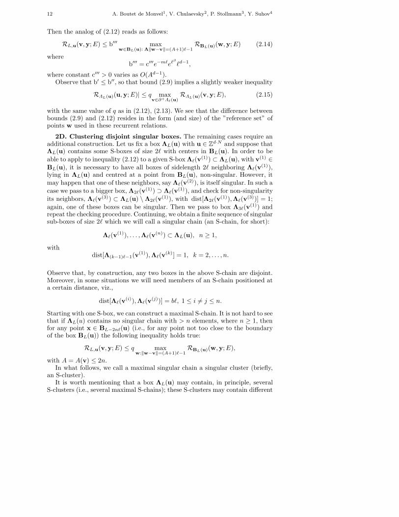
2D. Clustering disjoint singular boxes. The remaining cases require anadditional construction. Let us fix a box ΛL(u) with u ∈ Zd·N and suppose thatΛL(u) contains some S-boxes of size 2ℓ with centers in BL(u). In order to beable to apply to inequality (2.12) to a given S-box Λℓ(v

(1)) ⊂ ΛL(u), with v(1) ∈BL(u), it is necessary to have all boxes of sidelength 2ℓ neighboring Λℓ(v

(1)),lying in ΛL(u) and centred at a point from BL(u), non-singular. However, itmay happen that one of these neighbors, say Λℓ(v

(2)), is itself singular. In such acase we pass to a bigger box, Λ2ℓ(v

(1)) ⊃ Λℓ(v(1)), and check for non-singularity

its neighbors, Λℓ(v(3)) ⊂ ΛL(u) \ Λ2ℓ(v

(1)), with dist[Λ2ℓ(v(1)),Λℓ(v

(3))] = 1;again, one of these boxes can be singular. Then we pass to box Λ3ℓ(v

(1)) andrepeat the checking procedure. Continuing, we obtain a finite sequence of singularsub-boxes of size 2ℓ which we will call a singular chain (an S-chain, for short):

Λℓ(v(1)), . . . ,Λℓ(v

(n)) ⊂ ΛL(u), n ≥ 1,

withdist[Λ(k−1)ℓ−1(v

(1)),Λℓ(v(k)] = 1, k = 2, . . . , n.

Observe that, by construction, any two boxes in the above S-chain are disjoint.Moreover, in some situations we will need members of an S-chain positioned ata certain distance, viz.,

dist[Λℓ(v(i)),Λℓ(v

(j))] = bℓ, 1 ≤ i 6= j ≤ n.

Starting with one S-box, we can construct a maximal S-chain. It is not hard to seethat if ΛL(u) contains no singular chain with > n elements, where n ≥ 1, thenfor any point x ∈ BL−2nℓ(u) (i.e., for any point not too close to the boundaryof the box BL(u)) the following inequality holds true:

RL,u(v,y;E) ≤ q maxw:‖w−v‖=(A+1)ℓ−1

RBL(u)(w,y;E),

with A = A(v) ≤ 2n.In what follows, we call a maximal singular chain a singular cluster (briefly,

an S-cluster).It is worth mentioning that a box ΛL(u) may contain, in principle, several

S-clusters (i.e., several maximal S-chains); these S-clusters may contain different


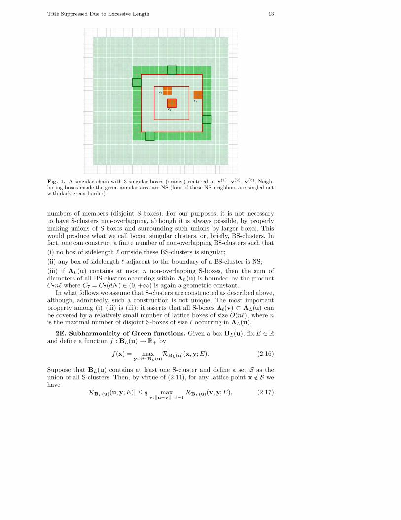
Fig. 1. A singular chain with 3 singular boxes (orange) centered at v(1), v(2), v(3). Neigh-boring boxes inside the green annular area are NS (four of these NS-neighbors are singled outwith dark green border)

numbers of members (disjoint S-boxes). For our purposes, it is not necessaryto have S-clusters non-overlapping, although it is always possible, by properlymaking unions of S-boxes and surrounding such unions by larger boxes. Thiswould produce what we call boxed singular clusters, or, briefly, BS-clusters. Infact, one can construct a finite number of non-overlapping BS-clusters such that

(i) no box of sidelength ℓ outside these BS-clusters is singular;

(ii) any box of sidelength ℓ adjacent to the boundary of a BS-cluster is NS;

(iii) if ΛL(u) contains at most n non-overlapping S-boxes, then the sum ofdiameters of all BS-clusters occurring within ΛL(u) is bounded by the productC7nℓ where C7 = C7(dN) ∈ (0,+∞) is again a geometric constant.

In what follows we assume that S-clusters are constructed as described above,although, admittedly, such a construction is not unique. The most importantproperty among (i)–(iii) is (iii): it asserts that all S-boxes Λℓ(v) ⊂ ΛL(u) canbe covered by a relatively small number of lattice boxes of size O(nℓ), where nis the maximal number of disjoint S-boxes of size ℓ occurring in ΛL(u).

2E. Subharmonicity of Green functions. Given a box BL(u), fix E ∈ R

and define a function f : BL(u) → R+ by

f(x) = maxy∈∂−BL(u)

RBL(u)(x,y;E). (2.16)

Suppose that BL(u) contains at least one S-cluster and define a set S as theunion of all S-clusters. Then, by virtue of (2.11), for any lattice point x 6∈ S wehave

RBL(u)(u,y;E)| ≤ q maxv: ‖u−v‖=ℓ−1

RBL(u)(v,y;E), (2.17)


while for points x ∈ S we have, respectively,

RBL(u)(u,y;E)| ≤ q maxv: ℓ≤‖u−v‖=2ℓ−1

RBL(u)(v,y;E), (2.18)

with the same value of q. Obviously, if S = ∅, then Eqn (2.17) can be used forall ℓ-boxes inside BL(u), which only makes our estimates simpler.

In order to formalize such a property of a function f , we give the following

Definition 2.2. Consider a box BL(u) and a subset thereof S ⊂ BL(u). Afunction f : BL(u) → R+ is called (q, ℓ,S)-subharmonic if for all points x ∈BL(u) \ S with dist[x, ∂−BL(u)] ≥ ℓ we have

f(x) ≤ q maxw: ‖w−x‖=2ℓ−1

f(w), (2.19)

and for every point x ∈ S there exists an integer ρ(x) ∈ [ℓ, Aℓ] and

f(x) ≤ q maxw: ρ(x)≤‖w−x‖≤ρ(x)+2ℓ−1

f(w). (2.20)

Remark. It is clear that, formally, we introduce the notion of (ℓ, q,S, A)-subharmonicity. The parameter A is dropped for notational simplicity only, andthis should not lead to any ambiguity.

We see that under the above assumptions upon the box BL(u), the function

f(x) := maxy∈∂−BL(u)

RBL(u)(x,y;E)

is (q, ℓ,S)-subharmonic with S defined as a union of all singular clusters and

q = e−γ(m,ℓ)eℓβ

C′(d)(nℓ)d−1.

Moreover, it is not difficult to see that if any family of disjoint singular boxes

Bℓ(v(1)),Bℓ(v

(2)), . . . ,Bℓ(v(j)) ⊂ BL(u)

contains at most n elements, i.e. j ≤ n, then the above function f is (q, ℓ,S)-subharmonic with some set S (which is not defined in a unique way, in general)contained in a union of annular areas

A(S) :=

j⋃

i=1

Ai, Ai = Bbi(u) \ Bai

(u)

with 0 < a1 < b1 < a2 . . . < aj < bj < L, W (S) :=∑j

i=1(bi − ai) ≤ 2nℓ. We willcall W (S) the (total) width of the singular area A(S). If the annular coveringA(S) is chosen in a minimal way, then W (S) is uniquely defined.

In the next subsection, we will establish a general bound for subharmonicfunctions, making abstraction of exact values of parameter q.

2.1. Radial descent and decay of subharmonic functions. The following elemen-tary statement is an adaptation of Lemma 4.3 from [C08]

Lemma 2.1. [Radial Descent Lemma]

f(u) ≤ q(L−W (S)−3ℓ)/ℓM(f,BL(u)). (2.21)

The proof can be found in [C08]; it is fairly straightforward.


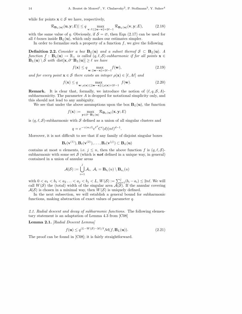
Fig. 2. An example of a box BL(u) with two singular clusters (singular boxes are orange)covered by two annular areas (pink)

2.2. Application to the decay of Green functions. It is readily seen that Lemma2.1 applied to the functions f(u) = R(u,v;E) leads to the following

Lemma 2.2. Fix a non-negative integer n <∞ and suppose that a box BL(u) isE-non-resonant and that any maximal family of b-distant (E,m)-singular boxescontains at most n elements. Then BL(u) is (m,E)-non-singular:

maxy∈∂−BL(u)

|GBL(u)(u,y;E)| ≤ exp −γ(m,L) .

N.B.: It is clear from our above analysis that all arguments, as well as thestatement of Lemma 2.2, remain valid for N -particle boxes in R

d (resp., two-particle boxes in Zd·N . Indeed, apart from the difference in the value of thedimension and the additive structure of the potential V(x1, x2) = V (x1)+V (x2),the two-particle Hamiltonians similar form. Neither of these differences is crucialto our analysis, for the dimension can be arbitrary, and a particular structure ofthe potential is not used at all.

Note also that our analysis of (ℓ, q,S)-subharmonic functions is purely ”de-terministic” and does not rely upon any probabilistic assumption relative to therandom external potential V (x;ω).

This concludes our reduction of the deterministic part of the continuous MSAto the lattice version thereof. The rest of the proof of exponential decay of Greenfunctions is conducted in terms of the auxiliary lattice model. The exponentialdecay of eigenfunctions is then deduced from that of Green functions in a stan-dard way. A reader familiar with [CS09A] may notice that subsequent sectionsare straightforward adaptations of corresponding parts of [CS09A]; they do notcontain truly novel ideas or techniques.


3. Partial decoupling and tunneling in two-particle boxes

Unlike the single-particle MSA, its two-particle counterpart proposed in [CS09A]has to address the following difficulty of multi-particle models: the probabilisticdependence between the values of the potential V(x;ω) = V (x1;ω) + V (x2;ω)and V(y;ω) = V (y1;ω) + V (y2;ω) does not decay with the distance ‖x − y‖.However, a weaker form of ”decoupling” in the potential U(x) + V(x;ω) takesplace for sufficiently distant points in the multi-particle configuration space. Sucha decoupling, sufficient for the purposes of the two-particle MSA, makes use ofthe following elementary geometric statement (cf. [CS09A]):

Lemma 3.1. Let be L > r0 and consider two interactive boxes, ΛL(u′) andΛL(u′′), with dist(ΛL(u′),ΛL(u′′)) > 8L. Then

ΠΛL(u′′) ∩ΠΛL(u′′) = ∅.

The proof is straightforward and can be found in [CS09A].

Further, for the purposes of estimates of probability of simultaneous (E,m)-singularity of two 8L-distant boxes, making use of well-known results of thesingle-particle MSA, we introduce the following

Definition 3.1. Given a bounded interval I ⊂ R and m > 0, a single-particlebox ΛLk

(u) is called m-tunneling (m-T, for short) if ∃E ∈ I and disjoint boxesΛLk−1

(v1), ΛLk−1(v2) ⊂ ΛLk

(u) which are (E,m)-S. A two-particle box of theform ΛLk

(u) = ΛLk−1(u1)×ΛLk−1

(u2), with u = (u1, u2), is called m-tunneling(m-T) if either ΛLk−1

(u1) or ΛLk−1(u2) is m-tunneling. Otherwise, it is called

m-non-tunneling (m-NT, for short).

It is worth mentioning that, while the notion of m-tunneling is, formally,defined for an arbitrary two-particle box, it is actually useful only in the case ofa non-interactive box, where the spectral problem admits separation of variables,and so is reduced to two single-particle spectral problems.

The following statement is a reformulation of well-known results of the single-particle MSA (cf. [St01] and bibliography therein), so its proof is omitted.

Lemma 3.2. Under the assumptions (E1–E4) upon the external (single-particle)external random potential V (x;ω),

P ΛLk(u) is m−T ≤ L−q′

k

where q′ = q′(η∗), η∗ := E∗1 − E∗

0 > 0, can be chosen so that q′(η∗) → +∞ asη∗ ↓ 0. Respectively, for a two-particle box ΛLk

(u) = ΛLk−1(u1)×ΛLk−1

(u2) wehave

P ΛLk(u) is m−T ≤

2∑

j=1

P ΛLk(uj) is m−T ≤ 2L−q′

k .


4. Reduction of the localization problem to the MSA

Theorem 4.1. Suppose that for some m > 0 and all k ≥ 0 the following boundholds true: for any pair of Lk-distant two-particle boxes BLk

(u′) and BLk(u′′),

P ∃E ∈ [E∗0 , E

∗1 ] : BLk

(u′) and BLk(u′′) are (E,m)-S ≤ L−2p

k . (4.1)

Then with probability one, the spectrum of operator H(ω) in [E∗0 , E

∗1 ] is pure

point, and for any EF Ψj(x;ω) with Ej(ω) ∈ [E∗0 , E

∗1 ], we have, for any v ∈

Zd·N :‖1C(v) Ψj(·;ω)| ≤ Cj(ω)e−m‖v‖. (4.2)

For the reader’s convenience, we give the proof of the above theorem in Section4. All its ingredients can be found in [CS09A] (as far as the two-particle structureof the Hamiltonian is concerned)) and in [St01].

Therefore, Anderson localization will be established, once we prove the mainprobabilistic bound of the MSA given by Eqn (4.1).

As usual in the MSA, the probabilistic bound (4.1) is first established fork = 0 initial length scale estimates), and then proved inductively for all k ≥ 1.

The proof of the initial length scale estimate is completely analogous to thatin the conventional, single-particle localization theory, and is omitted for thisreason. Indeed, the reader may check that the arguments used, e.g., in [St01] (cf.Ch. 3.3, pp. 90–98) do not use any assumption on the structure of the externalpotential which is not satisfied in the two-particle (actually, even N -particle,with N ≥ 1) model. The basis for these initial scale estimates is the well-knownCombes-Thomas bound (cf. [CT73]), combined with the fact that we considerenergies E ∈ [E∗

0 , E∗1 ] sufficiently close to the lower edge E∗

0 of the spectrum.So, in the rest of the paper, we focus on the inductive proof of the bound

(4.1). To this end, we consider two kinds of boxes:

(i) non-interactive boxes BL(u) = ΛL(u)∩Zd·N where the interaction potentialvanishes: U|ΛL(u) ≡ 0;

(ii) interactive boxes BL(u) = ΛL(u) ∩ Zd·N where the interaction potential is

not identically zero on ΛL(u).

This gives rise to three categories of pairs of (sufficiently distant) boxes:

(I) Two non-interactive boxes.

(II) Two interactive boxes.

(III) A mixed pair of one interactive and one non-interactive box.

These three cases will be treated separately in sections 5, 6 and 7, respectively.

By virtue of Theorem 4.1, Anderson localization (cf. Theorem 1) will beproven for the two-particle system in Rd with an alloy-type external randompotential, verifying conditions (D), (E1)-(E4) given in Section 1, once the bound(4.1) is established in all cases (I)-(III).

Remark. For the sake of notational simplicity, below we will call a box BL(u) =ΛL(u)∩Zd·N E-non-resonant (resp., E-non-resonant) iff the corresponding boxΛL(u) ⊂ Rd·N is E-resonant (resp., E-non-resonant).


5. Pairs of non-interactive boxes

We begin with an auxiliary result about non-interactive boxes, which was earlierused in [CS09A], [CS09B]. For the reader’s convenience, we give its proof (whichis straightforward) in the Appendix.

Lemma 5.1. Suppose that a two-particle box BLk+1(u) is E-non-resonant and

satisfies the following property: for any pair of sub-boxes BLk(v′),BLk

(v′) ⊂BLk+1

(u) with dist[BLk(v′),BLk

(v′′)] > 8Lk, either BLk(v′) or BLk

(v′) is(E,m)-non-singular. Then BLk+1

(u) is also (E,m)-non-singular.

Proof of (4.1) for a pair of non-interactive boxes.Consider a pair of two-particle non-interactive boxes B′ = BLk+1

(u′), B′′ =BLk+1

(u′′), and introduce the events

T = either Λ′ or Λ′′ is m-T ,R = ∃E ∈ [E0, E1] : both Λ′ and Λ′′ are E-R ,S = ∃E ∈ [E0, E1] : both Λ′ and Λ′′ are (E,m)-S .

Then we can writeP S ≤ P T + P S ∩ Tc .

Owing to Lemma 3.2, we have

P T ≤ P Λ′ is m-T + P Λ′′ is m-T ≤ 2 2L−q′

k ,

where q′ > 0 can be chosen arbitrarily large, provided that E∗1−E

∗0 is sufficiently

small. So, we can pick q′ ≥ q with q > 0 given in the Wegner-type bound (W2).Further, by two-volume Wegner-type estimate (W2), we have

P R < L−qk .

By virtue of the NITRoNS (Lemma 5.1), S ∩ Tc ⊂ R, Now, using (W2), weobtain

P S ≤ 4L−q′

k + P R ≤ L−q′

k + L−qk ≤ 2L−q

k < L−2pk ,

owing to our choice of parameter q(> 3p+ 9), for all sufficiently large Lk. Thus,the bound (4.1) is proven for distant pairs of non-interactive boxes.

6. Pairs of interactive boxes

Consider again the following events:

R = ∃E ∈ [E0, E1] : both B′ and B′′ are E-R ,S = ∃E ∈ [E0, E1] : both B′ and B′′ are (E,m)-S .

Using the Wegner-type bound (W2) and our condition q > 3p+ 9 , we see that

P S ≤ P R + P S ∩ Rc ≤1

2L−2p

k + P S ∩ Rc . (6.1)

Within the event Rc, either B′ or B′′ is E-non-resonant. Without loss of gener-ality, assume that B′ is E-non-resonant.


By virtue of the Radial Descent Lemma, if B′ is (E,m)-singular, but E-non-resonant, then it must contain a singular cluster of 2M + 1 ≥ 5 (with M = 2)distant sub-boxes BLk

(uj), j = 1, . . . , 2M + 1.Consider the following events:

S′I = B′ contains at least two (E,m)-S non-interactive boxes ,

S′NI = B′ contains at least 2M ≥ 4 (E,m)-S interactive boxes .

Obviously, S′ ⊂ S′I ∪ S′

NI .

Reasoning as in Section 5, we conclude that P S′I ≤ 2L−q

k .Further, suppose that B′ contains at least 2M (E,m)-singular distant interac-

tive boxes BLk(uj), j = 1, . . . , 2m. Owing to Lemma 3.1, the external potential

samples in boxes BLk(uj) are independent. The situation here is completely

analogous to that in the single-particle theory, and we can write that

P S′NI

≤ L2M(d+α−1)k+1

∏Mi=1 P ∃E ∈ [E0, E1] : BLk

(uj) and BLk(uj) are (E,m)-S

≤ L2M(d+α−1)k+1

(L−2p

k

)M

< 12L

−2pk+1,

as long as p > 3d2 +1, with M = 2, and L0 (hence, every Lk, k ≥ 1) is sufficiently

large. Taking into account Eqn (6.1), we see that

P S ≤1

2L−2p

k+1 +1

2L−2p

k+1 = L−2pk+1,

yielding the bound (4.1) for pairs of (distant) interactive boxes.

7. Mixed pairs of boxes

It remains to derive the bound (4.1) in case (III), i.e., for mixed pairs of two-particle boxes: an interactive box BLk+1

(x) and a non-interactive box BLk+1(y).

Here we use several properties which have been established earlier in this paperfor all scale lengths, namely, (W1), (W2), NITRoNS, and the bound (4.1) forpairs of (distant) non-interactive boxes, in Section 5.

Consider the following events:

S =∃E ∈ I : both BLk+1

(x), BLk+1(y) are (E,m)-S

,

T =

BLk+1(y) is m0-T

,

R =∃E ∈ I : neither BLk+1

(x) nor BLk+1(y) is (E, J)-NR

.

As before, we have

P T ≤ L−q′

k+1 ≤ L−qk+1, P R ≤ L−q

k+1. (5.3)

Further,

P S ≤ P T + P S ∩ Tc ≤1

4L−2p

k+1 + P S ∩ Tc ,


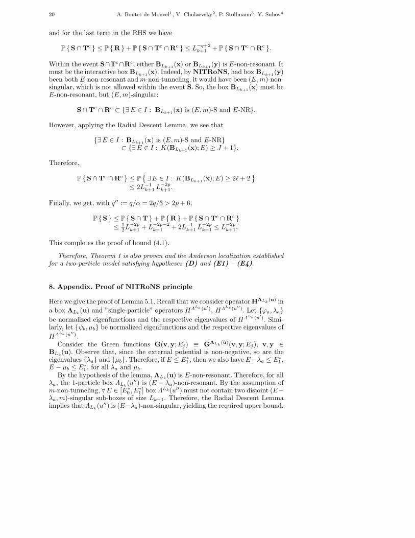
and for the last term in the RHS we have

P S ∩Tc ≤ P R + P S ∩ Tc ∩Rc ≤ L−q+2k+1 + P S ∩ Tc ∩ Rc .

Within the event S∩Tc∩Rc, either BLk+1(x) or BLk+1

(y) is E-non-resonant. Itmust be the interactive box BLk+1

(x). Indeed, by NITRoNS, had box BLk+1(y)

been both E-non-resonant andm-non-tunneling, it would have been (E,m)-non-singular, which is not allowed within the event S. So, the box BLk+1

(x) must beE-non-resonant, but (E,m)-singular:

S ∩ Tc ∩ Rc ⊂ ∃E ∈ I : BLk+1(x) is (E,m)-S and E-NR.

However, applying the Radial Descent Lemma, we see that

∃E ∈ I : BLk+1(x) is (E,m)-S and E-NR

⊂ ∃E ∈ I : K(BLk+1(x);E) ≥ J + 1.

Therefore,

P S ∩ Tc ∩ Rc ≤ P∃E ∈ I : K(BLk+1

(x);E) ≥ 2ℓ+ 2

≤ 2L−1k+1L

−2pk+1.

Finally, we get, with q′′ := q/α = 2q/3 > 2p+ 6,

P S ≤ P S ∩ T + P R + P S ∩Tc ∩ Rc

≤ 12L

−2pk+1 + L−2p−2

k+1 + 2L−1k+1L

−2pk+1 ≤ L−2p

k+1,

This completes the proof of bound (4.1).

Therefore, Theorem 1 is also proven and the Anderson localization establishedfor a two-particle model satisfying hypotheses (D) and (E1) – (E4).

8. Appendix. Proof of NITRoNS principle

Here we give the proof of Lemma 5.1. Recall that we consider operator HΛLk(u) in

a box ΛLk(u) and ”single-particle” operators HΛLk (u′), HΛLk (u′′). Let ϕa, λa

be normalized eigenfunctions and the respective eigenvalues of HΛLk (u′). Simi-larly, let ψb, µb be normalized eigenfunctions and the respective eigenvalues of

HΛLk (u′′).Consider the Green functions G(v,y;Ej) ≡ GΛLk

(u)(v,y;Ej), v,y ∈BLk

(u). Observe that, since the external potential is non-negative, so are theeigenvalues λa and µb. Therefore, if E ≤ E∗

1 , then we also have E−λa ≤ E∗1 ,

E − µb ≤ E∗1 , for all λa and µb.

By the hypothesis of the lemma, ΛLk(u) is E-non-resonant. Therefore, for all

λa, the 1-particle box ΛLk(u′′) is (E − λa)-non-resonant. By the assumption of

m-non-tunneling, ∀E ∈ [E∗0 , E

∗1 ] box ΛLk(u′′) must not contain two disjoint (E−

λa,m)-singular sub-boxes of size Lk−1. Therefore, the Radial Descent Lemmaimplies that ΛLk

(u′′) is (E−λa)-non-singular, yielding the required upper bound.


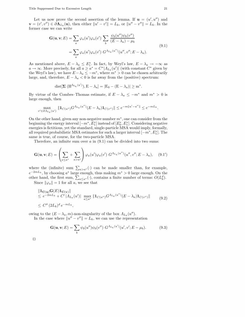
Let us now prove the second assertion of the lemma. If u = (u′, u′′) andv = (v′, v′′) ∈ ∂ΛLk

(u), then either ‖u′ − v′‖ = Lk, or ‖u′′ − v′′‖ = Lk. In theformer case we can write

G(u,v;E) =∑

a

ϕa(u′)ϕa(v′)∑

b

ψb(u′′)ψb(v

′′)

(E − λa) − µb

=∑

a

ϕa(u′)ϕa(v′) GΛLk(u′′)(u′′, v′′;E − λa).

(9.1)

As mentioned above, E − λa ≤ E∗1 . In fact, by Weyl’s law, E − λa → −∞ as

a→ ∞. More precisely, for all a ≥ a∗ = C∗|ΛLk(u′)| (with constant C∗ given by

the Weyl’s law), we have E−λa ≤ −m∗, where m∗ > 0 can be chosen arbitrarilylarge, and, therefore, E − λa < 0 is far away from the (positive) spectrum:

dist[Σ (HΛLk(u′)),E − λa] = |E0 − (E − λa)| ≥ m∗.

By virtue of the Combes–Thomas estimate, if E − λa ≤ −m∗ and m∗ > 0 islarge enough, then

maxv′∈∂ΛLk

(u′)‖1C(u′′)G

ΛLk(u′′)(E − λa)1C(v′′)‖ ≤ e−m‖u′−u′′‖ ≤ e−mLk .

On the other hand, given any non-negative numberm∗, one can consider from thebeginning the energy interval [−m∗, E∗

1 ] instead of [E∗0 , E

∗1 ]. Considering negative

energies is fictitious, yet the standard, single-particle MSA would imply, formally,all required probabilistic MSA estimates for such a larger interval [−m∗, E∗

1 ]. Thesame is true, of course, for the two-particle MSA.

Therefore, an infinite sum over a in (9.1) can be divided into two sums:

G(u,v;E) =

∑

a≤a∗

+∑

a>a∗

ϕa(u′)ϕa(v′) GΛLk

(u′′)(u′′, v′′;E − λa), (9.1′)

where the (infinite) sum∑

a>a∗(·) can be made smaller than, for example,

e−2mLk , by choosing a∗ large enough, thus making m∗ > 0 large enough. On theother hand, the first sum,

∑a≤a∗(·), contains a finite number of terms: O(Ld

k).

Since ‖ϕa‖ = 1 for all a, we see that

‖1C(u)G(E)1C(v)‖

≤ e−2mLk + C′ |ΛLk(u′)| max

a≤a∗‖1C(u′′)G

ΛLk(u′′)(E − λa)1C(v′′)‖

≤ C′′ (2Lk)d e−mLk ,

(9.2)

owing to the (E − λa,m)-non-singularity of the box ΛLk(u′′).

In the case where ‖u′′ − v′′‖ = Lk, we can use the representation

G(u,v;E) =∑

b

ψb(u′′)ψb(v

′′) GΛLk(u′)(u′, v′;E − µb). (9.3)

⊓⊔


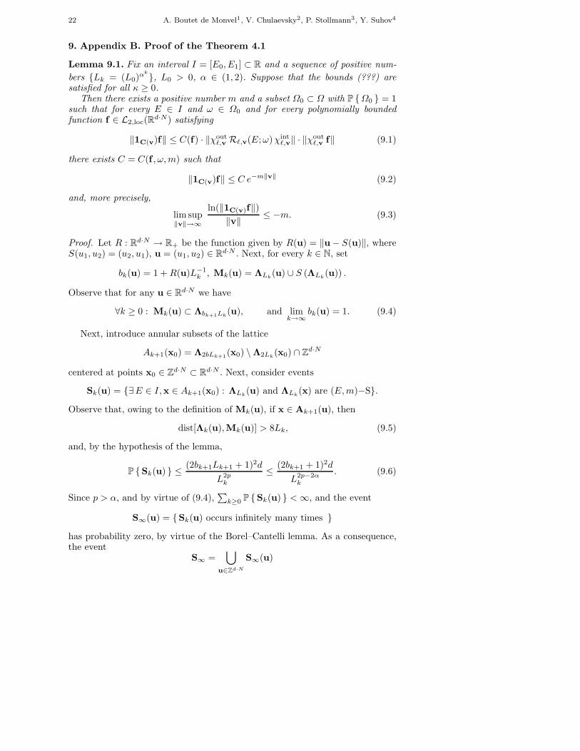
9. Appendix B. Proof of the Theorem 4.1

Lemma 9.1. Fix an interval I = [E0, E1] ⊂ R and a sequence of positive num-

bers Lk = (L0)αk

, L0 > 0, α ∈ (1, 2). Suppose that the bounds (???) aresatisfied for all κ ≥ 0.

Then there exists a positive number m and a subset Ω0 ⊂ Ω with P Ω0 = 1such that for every E ∈ I and ω ∈ Ω0 and for every polynomially boundedfunction f ∈ L2,loc(R

d·N) satisfying

‖1C(v)f‖ ≤ C(f) · ‖χoutℓ,v Rℓ,v(E;ω)χint

ℓ,v‖ · ‖χoutℓ,v f‖ (9.1)

there exists C = C(f , ω,m) such that

‖1C(v)f‖ ≤ C e−m‖v‖ (9.2)

and, more precisely,

lim sup‖v‖→∞

ln(‖1C(v)f‖)

‖v‖≤ −m. (9.3)

Proof. Let R : Rd·N → R+ be the function given by R(u) = ‖u− S(u)‖, whereS(u1, u2) = (u2, u1), u = (u1, u2) ∈ Rd·N . Next, for every k ∈ N, set

bk(u) = 1 +R(u)L−1k , Mk(u) = ΛLk

(u) ∪ S (ΛLk(u)) .

Observe that for any u ∈ Rd·N we have

∀k ≥ 0 : Mk(u) ⊂ Λbk+1Lk(u), and lim

k→∞bk(u) = 1. (9.4)

Next, introduce annular subsets of the lattice

Ak+1(x0) = Λ2bLk+1(x0) \ Λ2Lk

(x0) ∩ Zd·N

centered at points x0 ∈ Zd·N ⊂ Rd·N . Next, consider events

Sk(u) = ∃E ∈ I,x ∈ Ak+1(x0) : ΛLk(u) and ΛLk

(x) are (E,m)−S.

Observe that, owing to the definition of Mk(u), if x ∈ Ak+1(u), then

dist[Λk(u),Mk(u)] > 8Lk, (9.5)

and, by the hypothesis of the lemma,

P Sk(u) ≤(2bk+1Lk+1 + 1)2d

L2pk

≤(2bk+1 + 1)2d

L2p−2αk

. (9.6)

Since p > α, and by virtue of (9.4),∑

k≥0 P Sk(u) <∞, and the event

S∞(u) = Sk(u) occurs infinitely many times

has probability zero, by virtue of the Borel–Cantelli lemma. As a consequence,the event

S∞ =⋃

u∈Zd·N

S∞(u)


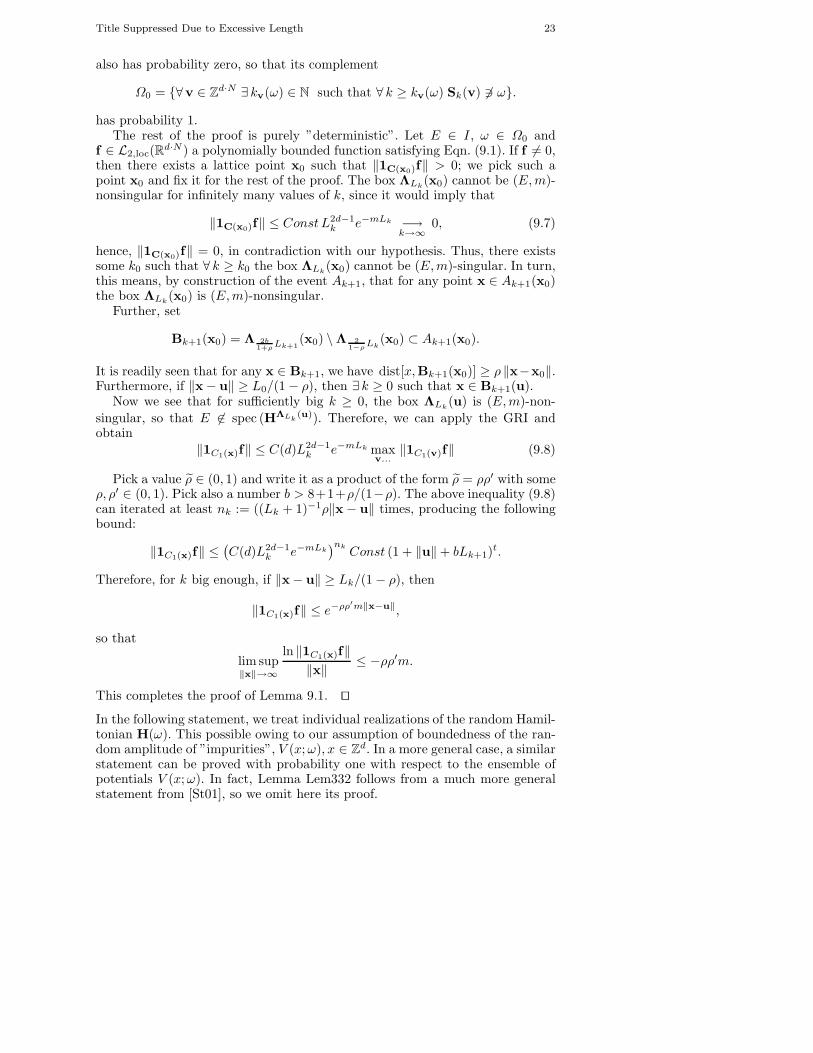
also has probability zero, so that its complement

Ω0 = ∀v ∈ Zd·N ∃ kv(ω) ∈ N such that ∀ k ≥ kv(ω) Sk(v) 6∋ ω.

has probability 1.The rest of the proof is purely ”deterministic”. Let E ∈ I, ω ∈ Ω0 and

f ∈ L2,loc(Rd·N ) a polynomially bounded function satisfying Eqn. (9.1). If f 6= 0,

then there exists a lattice point x0 such that ‖1C(x0)f‖ > 0; we pick such apoint x0 and fix it for the rest of the proof. The box ΛLk

(x0) cannot be (E,m)-nonsingular for infinitely many values of k, since it would imply that

‖1C(x0)f‖ ≤ ConstL2d−1k e−mLk −→

k→∞0, (9.7)

hence, ‖1C(x0)f‖ = 0, in contradiction with our hypothesis. Thus, there existssome k0 such that ∀ k ≥ k0 the box ΛLk

(x0) cannot be (E,m)-singular. In turn,this means, by construction of the event Ak+1, that for any point x ∈ Ak+1(x0)the box ΛLk

(x0) is (E,m)-nonsingular.Further, set

Bk+1(x0) = Λ 2b1+ρ

Lk+1(x0) \ Λ 2

1−ρLk

(x0) ⊂ Ak+1(x0).

It is readily seen that for any x ∈ Bk+1, we have dist[x,Bk+1(x0)] ≥ ρ ‖x−x0‖.Furthermore, if ‖x− u‖ ≥ L0/(1 − ρ), then ∃ k ≥ 0 such that x ∈ Bk+1(u).

Now we see that for sufficiently big k ≥ 0, the box ΛLk(u) is (E,m)-non-

singular, so that E 6∈ spec (HΛLk(u)). Therefore, we can apply the GRI and

obtain

‖1C1(x)f‖ ≤ C(d)L2d−1k e−mLk max

v...‖1C1(v)f‖ (9.8)

Pick a value ρ ∈ (0, 1) and write it as a product of the form ρ = ρρ′ with someρ, ρ′ ∈ (0, 1). Pick also a number b > 8+1+ρ/(1−ρ). The above inequality (9.8)can iterated at least nk := ((Lk + 1)−1ρ‖x − u‖ times, producing the followingbound:

‖1C1(x)f‖ ≤(C(d)L2d−1

k e−mLk)nk

Const (1 + ‖u‖ + bLk+1)t.

Therefore, for k big enough, if ‖x− u‖ ≥ Lk/(1 − ρ), then

‖1C1(x)f‖ ≤ e−ρρ′m‖x−u‖,

so that

lim sup‖x‖→∞

ln ‖1C1(x)f‖

‖x‖≤ −ρρ′m.

This completes the proof of Lemma 9.1. ⊓⊔

In the following statement, we treat individual realizations of the random Hamil-tonian H(ω). This possible owing to our assumption of boundedness of the ran-dom amplitude of ”impurities”, V (x;ω), x ∈ Zd. In a more general case, a similarstatement can be proved with probability one with respect to the ensemble ofpotentials V (x;ω). In fact, Lemma Lem332 follows from a much more generalstatement from [St01], so we omit here its proof.


Lemma 9.2. [Cf. Lemma 3.3.2 in [St01], Section 3.3] Assume that H(ω) satis-fies hypotheses (D) and (E1)–(E4). Then the following properties hold true:

(A) For spectrally almost every E ∈ Σ(H(ω)) there exists a polynomially boundedeigenfunction corresponding to E.

(B) For every bounded set I0 ⊂ R there exists a constant C = C(M, I0) such thatfor every generalized eigenfunction Ψ of H(ω) corresponding to E ∈ I0 satisfies

‖1C(u) Ψ‖ ≤ C ‖1C(w) (HΛ(ω) − E)−11C(u)‖ ‖1C(w) Ψ‖

where HΛ is the restriction of H(ω) to L2(Λ(u) with Dirichlet boundary condi-tions.

Now we are prepared to prove Theorem 4.1. Indeed, by Lemma 9.2, there isa set E0 ⊂ I = [0, E∗

0 ] with the following properties:

– ∀E ∈ E0 there is a polynomially bounded eigenfunction Ψ of H(ω) corre-sponding to E;

– I \ E0 is a set of measure zero for the spectral resolution of operator H(ω).

Further, by Lemma 9.1, every polynomially bounded generalized eigenfunc-tion Ψ corresponding to E ∈ I is exponentially decaying, in the L2-sense, and inparticular, Ψ ∈ L2(R

d·N ). This means that E is actually an eigenvalue. More-over, since the Hilbert space L2(R

d·N) is separable, this implies that the spec-trum of H(ω) is pure point and, as was just mentioned, all corresponding eigen-functions decay exponentially in the L2-sense, as stated in the Theorem 4.1. Thisconcludes the proof. ⊓⊔

Acknowledgments. The authors thank the organizers of the program ”Math-ematics and Physics of Anderson localization: 50 years after” at the Isaac New-ton Institute, University of Cambridge, for their hospitality. PS thanks the DFG(German Science Foundation) for financial support of visits to Paris and Cam-bridge.

References

[A94] M. Aizenman: Localization at weak disorder: elementary proofs. Rev. Math. Phys., 6,1162–1184 (1994).

[AGKW08] M. Aizenman, F. Germinet, A. Klein, S. Warzel, On Bernoulli decompositions forrandom variables, concentration bounds, and spectral localization. - Probab. Theory Relat.Fields, 143, 219–238, (2007).

[AW08] M. Aizenman, S. Warzel, Localization bounds for multiparticle systems. - Preprint,arXiv:math-ph/0809.3436, 2008; to appear in: Comm. Math. Phys.

[BCH97] J.M. Barbaroux, J.M. Combes, P.D. Hislop: Localization near band edges for randomSchrodinger operators. Helv. Phys. Acta, 70, 16–43 (1997).

[BK05] J. Bourgain, C. Kenig: On localization in the continuous Anderson-Bernoulli modelin higher dimension. Inv. Math., 161(2), 389–426 (2005).

[BCSS08A] A. Boutet de Monvel, V. Chulaevsky, P. Stollmann, Y. Suhov: Wegner-type boundsfor a two-particle continuous Anderson model with an alloy-type external potential. -arXiv:math-ph/0821.2621, 2008.

[BCSS08B] A. Boutet de Monvel, V. Chulaevsky, P. Stollmann, Y. Suhov: Wegner-type boundsfor a multi-particle continuous Anderson model with an alloy-type external potential. -submitted to Journ. Stat. Phys., 2008.

[C08] V. Chulaevsky: Localization with less larmes: simply MSA. - Preprint, arXiv:math-ph/0812.2634, 2008.


[CS08] V. Chulaevsky, Y. Suhov: Wegner bounds for a two-particle tight binding model. -Commun. Math. Phys., 283, 479–489 (2008).

[CS09A] V. Chulaevsky, Y. Suhov: Eigenfunctions in a two-particle Anderson tight bindingmodel. - Comm. Math. Phys., 289, 701–723 (2008); arXiv:math-ph/0810.2190, 2008.

[CS09B] V. Chulaevsky, Y. Suhov: Multi-particle Anderson localisation: induction on thenumber of particles. - Math. Phys. Anal. Geom., 12, 117–138 (2009); arXiv:math-ph/0811.2530, 2008.

[CH94] J.M. Combes, P.D. Hislop: Localization for some continuous, random Hamiltonians ind-dimensions, Journ. Funct. Anal., 124, 149–180 (1994).

[CT73] J.M. Combes, L. Thomas: Asymptotic behaviour of eigenfunctions for multiparticleSchrodinger operators, Comm. Math. Phys., 34, 251–270 (1973).

[DS01] D. Damanik, P. Stollmann: Multi-scale analysis implies strong dynamical localization,Geom. Funct. Anal. 11, 11–29 (2001).

[D87] H. von Dreifus: On the effect of randomness in ferromagnetic models and Schrodingeroperators. PhD thesis, New York University, 1987.

[DK89] H. von Dreifus, A. Klein: A new proof of localization in the Anderson tight bindingmodel. - Commun. Math. Phys., 124, 285–299 (1989).

[FS83] J. Frohlich, T. Spencer: Absence of diffusion in the Anderson tight binding model forlarge disorder or low energy. - Commun. Math. Phys., 88, 151–184 (1983).

[FMSS85] J. Frohlich, F. Martinelli, E. Scoppola, T. Spencer: A constructive proof of local-ization in Anderson tight binding model. - Comm. Math. Phys., 101, 21–46 (1985).

[GK01] F. Germinet, H. Klein: Bootstrap Multiscale Analysis and localization in randommedia. Commun. Math. Phys. 222(2), 415-448 (2001).

[GMP77] I.Ya. Goldsheid, S.A. Molchanov, L.A. Pastur: Typical one-dimensional Schrodingeroperator has pure point spectrum, Funktsional. Anal. i Prilozhen. 11 (1), 1–10 (1977);Engl. transl. in Functional Anal. Appl. 11 (1977).

[HM84] H.Holden and F.Martinelli: On the absence of diffusion for a Schrodinger operator onL

2(Rν) with a random potential. Commun. Math. Phys. 93, 197–217 (1984).[KSS98A] W. Kirsch, P. Stollmann, G. Stolz: Localization for random perturbations or peri-

odic Schrodinger operators. Random Operators and Stochastic Equations, 8(2), 153–180(1998).

[KSS98B] W. Kirsch, P. Stollmann, G. Stolz: Anderson localization for random Schrodingeroperators with long range interactions. Commun. Math. Phys. 195, 495–507 (1998).

[K95] F. Klopp: Localization for some continuous random Schrodinger operators. Commun.Math. Phys. 167, 553–569 (1995).

[KZ03] F. Klopp, H. Zenk: The integrated density of states for an interacting multielectron ho-mogeneous model. Preprint, Universite Paris-Nord, 2003; Adv. Math. Phys., 2009, ArticleID 6798727 (2009)

[S88] T. Spencer: Localization for random and quasiperiodic operators. - Journ. Stat. Phys.,51, No. 5/6, 1009–1019 (1988).

[St01] P. Stollmann, Caught by disorder. - Birkhauser, 2001.

Documents

Anderson localization in a multi-particle continuous model with … · Anderson localization in a multi-particle continuous model with an alloy-type external potential A. Boutet de