March 2010 RFF DP 10-15

Diversify or Focus? Spending to Combat Infectious Diseases When Budgets Are Tight

Soren An derson , Ramanan Laxminara yan , a nd S tephen W. Sa lan t

Diversify or Focus? Spending to Combat InfectiousDiseases When Budgets Are Tight∗

Soren Anderson†

Michigan State UniversityRamanan Laxminarayan‡

Resources for the Future

Stephen W. Salant§

University of MichiganResources for the Future

February 2, 2010

Abstract

We consider a health authority seeking to allocate annual budgets optimally over time tominimize the discounted social cost of infection(s) evolving in a finite set of R ≥ 2 groups.This optimization problem is challenging, since as is well known, the standard epidemi-ological model describing the spread of disease (SIS) contains a nonconvexity. Standardcontinuous-time optimal control is of little help, since a phase diagram is needed to addressthe nonconvexity and this diagram is 2R dimensional (a costate and state variable for eachof the R groups). Standard discrete-time dynamic programming cannot be used either,since the minimized cost function is neither concave nor convex globally. We modify thestandard dynamic programming algorithm and show how familiar, elementary argumentscan be used to reach conclusions about the optimal policy with any finite number of groups.We show that under certain conditions it is optimal to focus the entire annual budget onone of the R groups at a time rather than divide it among several groups, as is often donein practice; faced with two identical groups whose only difference is their starting level ofinfection, it is optimal to focus on the group with fewer sick people. We also show thatunder certain conditions it remains optimal to focus on one group when faced with a wealthconstraint instead of an annual budget.

∗For helpful comments and suggestions, we thank seminar participants at CIREQ. We also thank ZacharyStangebye for valuable research assistance.†sta@msu.edu or 517-355-0286‡ramanan@rff.org or 202-328-5085§ssalant@umich.edu or 734-223-7439

1 Introduction

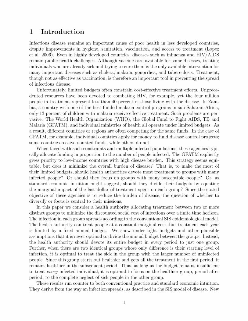
Infectious disease remains an important cause of poor health in less developed countries,despite improvements in hygiene, sanitation, vaccination, and access to treatment (Lopezet al. 2006). Even in highly developed countries, diseases such as influenza and HIV/AIDSremain public health challenges. Although vaccines are available for some diseases, treatingindividuals who are already sick and trying to cure them is the only available intervention formany important diseases such as cholera, malaria, gonorrhea, and tuberculosis. Treatment,though not as effective as vaccination, is therefore an important tool in preventing the spreadof infectious disease.

Unfortunately, limited budgets often constrain cost-effective treatment efforts. Unprece-dented resources have been devoted to combating HIV, for example, yet the four millionpeople in treatment represent less than 40 percent of those living with the disease. In Zam-bia, a country with one of the best-funded malaria control programs in sub-Saharan Africa,only 13 percent of children with malaria receive effective treatment. Such problems are per-vasive. The World Health Organization (WHO), the Global Fund to Fight AIDS, TB andMalaria (GFATM), and individual ministries of health all operate under limited budgets. Asa result, different countries or regions are often competing for the same funds. In the case ofGFATM, for example, individual countries apply for money to fund disease control projects;some countries receive donated funds, while others do not.

When faced with such constraints and multiple infected populations, these agencies typi-cally allocate funding in proportion to the number of people infected. The GFATM explicitlygives priority to low-income countries with high disease burden. This strategy seems equi-table, but does it minimize the overall burden of disease? That is, to make the most oftheir limited budgets, should health authorities devote most treatment to groups with manyinfected people? Or should they focus on groups with many susceptible people? Or, asstandard economic intuition might suggest, should they divide their budgets by equatingthe marginal impact of the last dollar of treatment spent on each group? Since the statedobjective of these agencies is to reduce the burden of disease, the question of whether todiversify or focus is central to their missions.

In this paper we consider a health authority allocating treatment between two or moredistinct groups to minimize the discounted social cost of infections over a finite time horizon.The infection in each group spreads according to the conventional SIS epidemiological model.The health authority can treat people at a constant marginal cost, but treatment each yearis limited by a fixed annual budget. We show under tight budgets and other plausibleassumptions that it is never optimal to divide the annual budget between the groups. Instead,the health authority should devote its entire budget in every period to just one group.Further, when there are two identical groups whose only difference is their starting level ofinfection, it is optimal to treat the sick in the group with the larger number of uninfectedpeople. Since this group starts out healthier and gets all the treatment in the first period, itremains healthier in the subsequent period. Thus, as long as the budget remains insufficientto treat every infected individual, it is optimal to focus on the healthier group, period afterperiod, to the complete neglect of sick people in the other group.

These results run counter to both conventional practice and standard economic intuition.They derive from the way an infection spreads, as described in the SIS model of disease. New

1

infections arise from healthy people interacting with the sick. Thus, treating one sick personnot only cures that single individual some percentage of the time but then also preventshealthy people from becoming infected at a later date. If there are many such healthypeople, then spending the money required to treat one sick person prevents much disease. Ifmany people are already sick, however, then treating one sick person prevents disease in fewerhealthy people, and the treated individual herself is more likely to become sick again. Thehealth authority in effect faces dynamic increasing returns to treatment in each group: thegreater the number of healthy people, the more effective treating sick people in the groupbecomes. Thus, when presented with multiple infected groups and a limited budget, thehealth authority should take advantage of increasing returns by devoting its entire budgetto a single group. Put differently, given the SIS dynamics, the health authority’s cost-minimization problem is concave, leading to a corner solution in every period.

Determining how best to minimize the burden of infectious disease calls for a combinationof epidemiological and economic insights, an approach taken in both the economics and theepidemiology literatures. Based on the pioneering work of Revelle (1967), Sanders (1971),and Sethi (1974), a more recent literature has emerged to clarify a number of importantissues associated with this dynamic optimization problem (Goldman and Lightwood 2002;Rowthorn and Brown 2003; Gersovitz and Hammer 2004; Smith et al. 2005; Gersovitz andHammer 2005; Herrmann and Gaudet 2009). None of these articles, however, describe theoptimal treatment of multiple populations when the health authority has a limited budget.

Most of the literature minimizes the discounted sum of treatment costs plus the socialcosts of the infection. As always, the solution to such a “planning problem” is a valuablebenchmark, since it identifies what is socially best. Often, however, health authorities inthe real world are unable to achieve this first-best outcome. An authority may be charged,for example, with minimizing forgone production (or school attendance) due to illness butmay lack the authority to tax or borrow. It then has no choice but to live within its annualbudget. Indeed, governmental ministries of health may be prohibited by law from borrowing,as are entities such as the GFATM. In our base case, we assume that no one will lend tothis health authority despite its promise to repay the loan out of its future annual budgets—perhaps because the health authority cannot precommit to repaying the loan in the future.To show that our results do not depend on this assumption, however, we also examine theless plausible case where the health authority can borrow against future budgets.1

The dynamic increasing returns to treatment inherent in the standard epidemiologicalmodel (SIS) make deriving the optimal treatment policy difficult, even for a single population.This nonconvexity in the planner’s cost-minimization problem has haunted the literaturefrom the outset. In an early paper, Sanders (1971) concludes that treatment should alwaysbe set to zero or the maximum possible level, but Sethi (1974), analyzing the same problem,concludes to the contrary that optimal treatment is always interior except in transitionalphases at the beginning and end of the program. More recently, Gersovitz and Hammer(2004) recognize that they cannot prove analytically that the solutions to their necessaryconditions are optimal, since, as they note, the standard sufficiency conditions fail in the

1This latter case involves the minimization of forgone production due to illness subject to any wealthconstraint of the health authority. It therefore includes the solution of the planning problem as a specialcase; it also includes the case where the constraint is so tight that, at the constrained optimum, spending adollar more in wealth would reduce the social cost of infection by more than a dollar.

2

presence of the nonconvexity (pp. 10 and 26). They instead rely on numerical simulationsto argue that their solutions are likely optimal.

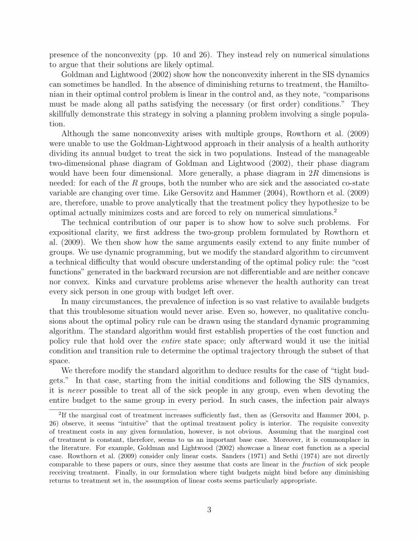
Goldman and Lightwood (2002) show how the nonconvexity inherent in the SIS dynamicscan sometimes be handled. In the absence of diminishing returns to treatment, the Hamilto-nian in their optimal control problem is linear in the control and, as they note, “comparisonsmust be made along all paths satisfying the necessary (or first order) conditions.” Theyskillfully demonstrate this strategy in solving a planning problem involving a single popula-tion.

Although the same nonconvexity arises with multiple groups, Rowthorn et al. (2009)were unable to use the Goldman-Lightwood approach in their analysis of a health authoritydividing its annual budget to treat the sick in two populations. Instead of the manageabletwo-dimensional phase diagram of Goldman and Lightwood (2002), their phase diagramwould have been four dimensional. More generally, a phase diagram in 2R dimensions isneeded: for each of the R groups, both the number who are sick and the associated co-statevariable are changing over time. Like Gersovitz and Hammer (2004), Rowthorn et al. (2009)are, therefore, unable to prove analytically that the treatment policy they hypothesize to beoptimal actually minimizes costs and are forced to rely on numerical simulations.2

The technical contribution of our paper is to show how to solve such problems. Forexpositional clarity, we first address the two-group problem formulated by Rowthorn etal. (2009). We then show how the same arguments easily extend to any finite number ofgroups. We use dynamic programming, but we modify the standard algorithm to circumventa technical difficulty that would obscure understanding of the optimal policy rule: the “costfunctions” generated in the backward recursion are not differentiable and are neither concavenor convex. Kinks and curvature problems arise whenever the health authority can treatevery sick person in one group with budget left over.

In many circumstances, the prevalence of infection is so vast relative to available budgetsthat this troublesome situation would never arise. Even so, however, no qualitative conclu-sions about the optimal policy rule can be drawn using the standard dynamic programmingalgorithm. The standard algorithm would first establish properties of the cost function andpolicy rule that hold over the entire state space; only afterward would it use the initialcondition and transition rule to determine the optimal trajectory through the subset of thatspace.

We therefore modify the standard algorithm to deduce results for the case of “tight bud-gets.” In that case, starting from the initial conditions and following the SIS dynamics,it is never possible to treat all of the sick people in any group, even when devoting theentire budget to the same group in every period. In such cases, the infection pair always

2If the marginal cost of treatment increases sufficiently fast, then as (Gersovitz and Hammer 2004, p.26) observe, it seems “intuitive” that the optimal treatment policy is interior. The requisite convexityof treatment costs in any given formulation, however, is not obvious. Assuming that the marginal costof treatment is constant, therefore, seems to us an important base case. Moreover, it is commonplace inthe literature. For example, Goldman and Lightwood (2002) showcase a linear cost function as a specialcase. Rowthorn et al. (2009) consider only linear costs. Sanders (1971) and Sethi (1974) are not directlycomparable to these papers or ours, since they assume that costs are linear in the fraction of sick peoplereceiving treatment. Finally, in our formulation where tight budgets might bind before any diminishingreturns to treatment set in, the assumption of linear costs seems particularly appropriate.

3

lies within a given rectangular region. We establish that each cost function is strictly con-cave over this rectangular region; the irregularities in the cost function that undermine thestandard algorithm arise elsewhere in the state space. Since no feasible treatment programcan result in infection combinations outside this rectangular region, the curvature of thecost function outside the region is irrelevant. A similar argument may be useful in otherdynamic programming problems for which qualitative conclusions about the optimal policyseem elusive.

The remainder of the paper is organized as follows. In section 2, we consider the problemof a health authority allocating funds over time to minimize the discounted sum of social costsof infection in two groups. Throughout this section, we assume that the health authorityreceives an annual budget and can neither borrow against it nor save funds for the future.In section 3, we show how our arguments generalize when the health authority allocatesits budget across R > 2 groups. We then relax the constraint on borrowing and saving insection 4. Section 5 concludes the paper. Throughout, we assume that those infected in onegroup cannot transmit their disease to members of another group. Therefore, our analysisapplies both to cases where every group faces the same disease, as well as to cases where thediseases in some (or all) of the groups are different.

2 The Health Authority’s problem

2.1 Assumptions

Infectious diseases are spreading within two distinct groups. The spread of each infection isgoverned by the following difference equations:

I it+1 = (1− µi)I it + θiI itN i

(N i − I it)− αiF it (1)

where parameters µi, θi, N i, αi > 0 for groups i = A,B. The population size of group iis fixed at N i. The number of infected individuals (infecteds) in period t is I it and thenumber of healthy individuals (susceptibles) is N i− I it . The number of individuals in groupi treated in period t is F i

t . We interpret µi as the fraction of infected individuals in groupi who spontaneously recover (whether or not they were treated), θiI it/N

i as the fraction ofsusceptibles that become infected (which is proportional to the fraction infected), and αi asthe fraction of those treated individuals whom the treatment cures (excluding those treatedwho would have recovered spontaneously so as to avoid double counting). Mathematically,each group’s infection level is independent of the other’s, which implies that the infectionsdo not spread between the groups. In this case, different diseases can be afflicting the twogroups.

We assume that the cost of treating each infected individual in group i is constant pi andthat the health authority has an annual budget in period t of Mt. The health authority canneither borrow against its budget nor save funds for the future. The budget constraint inperiod t is therefore

pAFAt + pBFB

t ≤Mt, (2)

4

for all t = 1, ..., T ; we relax this assumption in Section 4. And we assume that the treatmentis never used as a prophylactic, so only infected individuals receive it:

0 ≤ F it ≤ I it (3)

for i = A,B and all t = 1, ..., T .To streamline the notation, let

Γi(I it) ≡ (1− µi)I it + θiI itN i

(N i − I it) (4)

denote the number of infections in group i in period t+1 if there were I it infecteds in period tand none received treatment. Then the spread of the infection in group i can be re-expressedas

I it+1 = Γi(I it)− αiF it (5)

for i = A,B. For most of the paper we suppress further mention of the specific functionalform in (1) above. Thus, all of our results will hold for the generic functional form in (5),subject to a handful of regularity assumptions that we detail immediately below.

We impose several restrictions on the infection dynamics. First, we assume that Γi(I it)−αiI it is strictly increasing in I it for all I it ∈ [0, N i] for i = A,B. That is, if every infectedindividual received treatment, the more infected people there are in the current period, themore there would be in the next period. As we show below, this assumption guaranteesthat the cost function is increasing, which implies that it is always optimal to exhaust thebudget.3 It follows from this assumption that Γi(I it) is also increasing for all I it ∈ [0, N i] fori = A,B.

Second, we assume that Γi(I it) is strictly concave for all I it ∈ [0, N i] for i = A,B. ThatΓ(·) is concave when we impose our specific functional form is clear from the second derivative

−2θi

N i < 0 and requires no further assumptions in that special case.Third, we assume that Γi(0) = 0 and that Γi(N i) ≤ N i for i = A,B, which, given our

other assumptions, implies that infection levels in each group are always nonnegative andnever exceed either group’s population:

0 ≤ I it ≤ N i (6)

for i = A,B and all t = 1, ..., T .4

Finally, we make the following simplifying assumption: even if the health authoritydevoted its entire budget in every period to the same group (either A or B), it would neverhave enough funds to treat all the infected individuals in that group. Hence, no matter howthe health authority behaves,

3Given the specific functional form we present above, this assumption reduces to a restriction on the firstderivative evaluated at Iit = N i:

1− µi − θi − αi > 0,

for i = A,B.4It is clear that Γi(0) = 0 for our specific functional form. The assumption that Γi(N i) ≤ N i holds as long

as µi ∈ [0, 1] for i = A,B: given an infection level of Iit ∈ [0, N i] in period t, the minimum number of infectedsin period t+ 1 would be Γi(0)− αi · 0 = 0, while the maximum would be Γi(N i) = (1− µi)N i ∈ [0, N i].

5

Mt

pB

NB

IBt

NAMt

pA IAt

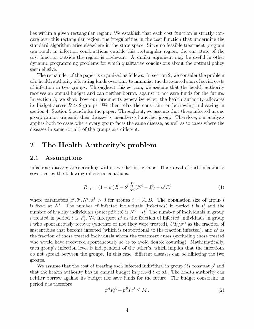
Figure 1: Period t’s rectangle

Note: Assumption 1 is that it is never possible to treat all the sick people in eithergroup. Thus, infection pairs in period t must lie within the rectangular region identifiedin the figure. Given assumption 1, we are able to establish concavity of the cost functionover this rectangular region.

Assumption 1. N i ≥ I it ≥ Mt

pi for i = A,B for all t = 1, 2, ..., T .

It follows that, in period t, the infection pair must lie in a rectangular region of heightNB − Mt

pB and length NA − Mt

pA . We refer to this as “period t’s rectangle.” See Figure 1.Assumption 1 is not necessary in some cases for our result but seems realistic and simplifiesthe analysis.

2.2 Cost-minimization problem

The health authority chooses how many individuals to treat in each group in every periodt = 1, ..., T , subject to constraints (2) and (3) above, to minimize the discounted sum of thesocial costs of infection in the two groups:

T∑t=1

δt−1[sAIAt + sBIBt ],

where T indexes the final period, si denotes the social cost per infected person in group i,and δ ∈ (0, 1) denotes the discount factor. We assume that infection levels initially are IA1

6

and IB1 and thereafter follow the relevant difference equation in (1) (or equation (5), the caseof a generic functional form).

It is convenient to express the health authority’s problem recursively. Denote the mini-mized cost of entering period t+ 1 with infection pair (IAt+1, I

Bt+1) and proceeding optimally

thereafter as Ct+1(IAt+1, IBt+1).5 The cost function for period t therefore is given by

Ct(IAt , I

Bt ) = min

FAt ,F

Bt

sAIAt + sBIBt + δCt+1(ΓA(IAt )− αAFAt ,Γ

B(IBt )− αBFBt )

subject to pAFAt + pBFB

t ≤Mt and FAt , F

Bt ≥ 0.

2.3 Three-period problem

To build intuition, we begin by determining what the health authority should do in the lastthree periods (T − 2, T − 1, and T ). Since spending at T has no effect on social costs untilafter the end of the horizon, it is optimal to spend nothing then (F i

T = 0) and CT (IAT , IBT ) =

sAIAT + sBIBT . As for the optimal decision at T − 1, the social cost of infection is a linear,strictly decreasing function of the number of individuals (FA

T−1, FBT−1) treated in each group.

Hence, it will be optimal to spend the entire budget on only one group.More formally, the health authority wants to allocate its budget at T − 1 to minimize

the discounted social cost of infection from that period onward:

CT−1(IAT−1, IBT−1) = min

FAT−1,F

BT−1

sAIAT−1 + sBIBT−1

+δ[sAΓA(IAT−1)− sAαAFAT−1 + sBΓB(IBT−1)− sBαBFB

T−1] (7)

subject to FAT−1, F

BT−1 ≥ 0 and pAFA

T−1 + pBFBT−1 ≤MT−1.

The constraint set is a familiar budget triangle, with boundary slope − pA

pB . The slopeindicates the number of additional infected individuals in group B who can be treated usingthe money saved by not treating one individual in group A.6 The preference direction isalso conventional (northeast), since treating more individuals in either group reduces thediscounted sum of social costs of infection in the two groups. The indifference curves aredownward-sloping lines with MRS = −αAsA

αBsB < 0. So the health authority should spend its

5We have suppressed the dependence of minimized costs on future budget levels and various fixed param-eters to simplify the notation.

6Assumption 1 ensures that all treatment pairs in the budget triangle are feasible. If Assumption 1 wereviolated, there could be money left over after treating every infected individual in one group. In that case,treatment pairs in one (or both) corners of the triangle would be deemed inadmissible, since the healthauthority does not treat susceptibles prophylactically. That is, the constraint set is the intersection of threeconstraints: the budget set and F it ≤ Iit for i = A,B. Assumption 1 guarantees that these additionalconstraints never bind and can be disregarded. If Assumption 1 is violated, the optimum might occur whereF it = Iit <

Mt

pi . In that case, funds remaining would be spent on the other group. This not only increasesthe number of cases that must be considered but also results in a minimized cost function that is notconcave everywhere. That the health authority never serves both groups (unless it has treated every infectedindividual in one group) can still be established in the only case we have examined (the symmetric case).But concavity arguments no longer work, and the proof instead relies on a property of the cost functionthat seems of limited applicability to other problems. The proof for the symmetric case in the absence ofAssumption 1 is available upon request.

7

entire budget on group A if αAsA

pA > αBsB

pB and on group B if αAsA

pA < αBsB

pB . If neither inequal-ity holds, then the health authority is indifferent between spending on infected individualsin either group and any combination of treatment that exhausts the budget is optimal. In-

tuitively, by treating one less individual in group A, the health authority can treat pA

pB moreindividuals in group B. If one less individual is treated in group A, discounted social costs

there would increase by αAsA; if pA

pB more individuals are treated in group B, social costs

there would decrease by αBsB pA

pB . This reallocation is beneficial if the result is a net reduc-

tion in discounted social costs from that period onward (αBsB pA

pB − αAsA > 0); if, instead,it raises social costs, then the arbitrage should be reversed. Reallocating toward group A isoptimal if (1) the price of treatment (pA) in group A is sufficiently low, (2) the effectivenessof the treatment (αA) in group A is sufficiently high, or (3) the social cost of infection (sA)in group A is sufficiently high.

The decision in period T − 1 of how many individuals in each group to treat is straight-forward because the only cost consequences occur in period T. When the decision is made insome prior period, however, the health authority should take into account the discountedcost consequences from the next period onward of reallocating the current budget. To de-duce these consequences, the authority needs to compute the sequence of minimized costfunctions.

We can compute the minimized cost function in period T −1 by substituting the optimaldecision rule (FA

T−1, FBT−1) into the objective function in equation (13):

CT−1(IAT−1, IBT−1) = sAIAT−1 + sBIBT−1

+δ

[sAΓA(IAT−1) + sBΓB(IBT−1)−MT−1 max

(αAsA

pA,αBsB

pB

)]. (8)

The cost function CT−1(IAT−1, IBT−1) is the sum of continuous functions and is therefore contin-

uous. Since Γi(·) is strictly increasing in its single argument (for i = A,B), CT−1(IAT−1, IBT−1)

is strictly increasing in its two arguments. Moreover, since Γi(·) is strictly concave in itssingle argument and the right-hand side of (8) is additively separable, CT−1(IAT−1, I

Bt−1) is

strictly jointly concave (henceforth, simply “strictly concave”) in (IAT−1, IBT−1). As we will

show, prior minimized cost functions inherit these two properties; each is strictly increasingand strictly concave.

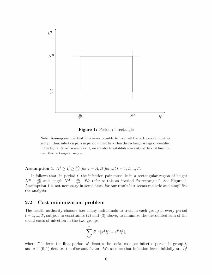
The health authority allocates its budget at T − 2 to minimize the discounted social costof infection from that period onward:

CT−2(IAT−2, IBT−2) = min

FAT−2,F

BT−2

sAIAT−2 + sBIBT−2

+δCT−1(ΓA(IAT−2)− αAFAT−2,Γ

B(IBT−2)− αBFBT−2) (9)

subject to FAT−2, F

BT−2 ≥ 0 and pAFA

T−2 + pBFBT−2 ≤ MT−2. Since the constraint set is

compact and the minimand is continuous, an optimal allocation rule for the budget atT − 2 exists (Weierstrass Theorem) and the minimum value function CT−2(·, ·) is itselfcontinuous (Berge’s Theorem).7 Admissible allocations of the period T − 2 budget between

7Proceeding inductively, it is straightforward to establish that an optimal budget allocation rule exists ateach stage.

8

FBT−2

FAT−2

MBT−2pB

MAT−2pA

decreasing socialdiscounted cost

period T − 2budget triangle

cost-minimizingindifference curve

Figure 2: Allocation of the health budget in period T − 2and its consequences for social cost

the two groups lie in a right-triangle with hypotenuse of slope - pA

pB . See Figure 2. The locusof expenditures across the two groups that results in a given discounted social cost fromthe current period onward is an “indifference curve.” The indifference curve is downwardsloping, since spending more on either group would lower the discounted social cost. Budgetallocations to the “southwest” of the indifference curve (including the origin, where nothing isspent on the sick of either group) result in strictly higher social cost while budget allocationsto the “northeast” result in strictly lower social cost. Since CT−1(IAT−1, I

BT−1) is strictly

concave in the infection pair, it is strictly concave in the pair of health expenditures and mustbe strictly quasi-concave in them as well. Hence, budget allocations resulting in a strictlyhigher discounted social cost must form a strictly convex set, and the optimal allocation ofthe health budget requires spending the entire health budget at T − 2 on a single group.8

8The marginal rate of substitution between FAT−2 and FBT−2 is:

dFBT−2

dFAT−2

= −(δαA + δ2αAΓA′(ΓA(IAT−2)− αAFAT−2))sA

(δαB + δ2αBΓB ′(ΓB(IBT−2)− αBFBT−2))sB, (10)

which is strictly negative since Γi(·) is strictly increasing for i = A,B. Since Γi(·) is also strictly concave,the magnitude of the MRS strictly increases as one moves downward along any indifference curve (as FAT−2

increases and FBT−2 decreases). That is, the indifference curves are strictly concave.

9

2.4 Problem of any finite length

With any finite number of periods, the health authority chooses FAt , F

Bt ≥ 0 to minimize

sAIAt + sBIBt + δCt+1

(ΓA(IAt )− αAFA

t ,ΓB(IBt )− αBFB

t

)(11)

subject to the budget constraint pAFAt +pBFB

t ≤Mt. We will show that the cost function inevery period (t = 1, . . . T − 1) is both strictly increasing and strictly concave in its inheritedinfection levels. This in turn implies that in every period the health authority will devoteits entire budget to either one group or the other.

We begin by showing that the cost function is strictly increasing in every period.

Theorem 1. The cost function Ct(IAt , I

Bt ) is strictly increasing for any I it ∈ [Mt

pi , Ni] where

i = A,B, and t = 1, 2, ..., T .

Proof. First recall that the cost function at T −1, CT−1(IAT−1, IBT−1), is strictly increasing for

any infection levels (IAT−1, IBT−1) in the period T − 1 rectangle. Now assume inductively that

in any period t < T − 1 the cost function starting in the subsequent period Ct+1(IAt+1, IBt+1)

is strictly increasing for any infection levels (IAt+1, IBt+1) in the period t+ 1 rectangle. We will

show that the cost function starting in period t given by Ct(IAt , I

Bt ) is strictly increasing for

any infection levels (IAt , IBt ) in the period t rectangle.

Let

Ω(IAt , IBt , F

At , F

Bt ) ≡ sAIAt + sBIBt + δCt+1

(ΓA(IAt )− αAFA

t ,ΓB(IBt )− αBFB

t

)(12)

denote the objective function that the health authority minimizes. Note that by hypothesisCt+1(IAt+1, I

Bt+1) is strictly increasing for (IAt+1, I

Bt+1) in the period t + 1 rectangle and that

Γi(I it) is strictly increasing in I it for i = A,B. Thus, Ω(IAt , IBt , F

At , F

Bt ) is strictly increasing

for any infection pair (IAt , IBt ) in the period t rectangle. Let (FA

t , FBt ) be the cost-minimizing

treatment levels given initial infection levels (IAt , IBt ) in the period t rectangle. Consider any

smaller infection pair (IAt , IBt ) in the period t rectangle such that IAt > IAt and IBt = IBt ,

so that the infection pair is strictly smaller in the direction of IAt . Then the minimizeddiscounted social cost from period t onward of entering period t with a strictly smallerinfection pair is strictly smaller. That is,

Ct(IAt , I

Bt ) = Ω(IAt , I

Bt , F

At , F

Bt )

> Ω(IAt , IBt , F

At , F

Bt )

≥ Ct(IAt , I

Bt ),

where equality in the first line follows from the definition of the cost function, the inequalityin the second line follows from the fact that the minimand is an increasing function of initialinfection levels, and the inequality in the third line follows from cost minimization. So thecost function is strictly increasing for any IAt ∈ [Mt

pA , NA]. A symmetric argument establishes

that it is also strictly increasing for any IBt ∈ [Mt

pB , NB].9

9We could show that the cost function is strictly increasing over a wider range of infection levels, butthe proof of our key result below relies on concavity, which we are only able to establish over the period trectangle.

10

Next we show that the cost function in every period is strictly concave over the rectangularregion identified in assumption 1.

Theorem 2. The cost function Ct(IAt , I

Bt ) is strictly concave for any I it ∈ [Mt

pi , Ni] where

i = A,B, and t = 1, 2, ..., T − 1.

Proof. Recall that CT−1(IAT−1, IBT−1), defined in equation (8), is strictly concave for any

(IAT−1, IBT−1) in the period T − 1 rectangle. Now assume inductively that in any period

t < T − 1 the cost function starting in the subsequent period Ct+1(IAt+1, IBt+1) is strictly con-

cave for any (IAt+1, IBt+1) in the period t + 1 rectangle. We will show that the cost function

starting in period t given by Ct(IAt , I

Bt ) is strictly concave for any (IAt , I

Bt ) in the period t

rectangle.As before, let

Ω(IAt , IBt , F

At , F

Bt ) ≡ sAIAt + sBIBt + δCt+1

(ΓA(IAt )− αAFA

t ,ΓB(IBt )− αBFB

t

)be the function that the health authority minimizes. Note that if Ct+1(IAt+1, I

Bt+1) is strictly

concave in (IAt+1, IBt+1) for any infection pair in the period t+1 rectangle, then Ω(IAt , I

Bt , F

At , F

Bt )

is strictly concave for any (IAt , IBt ) in the period t rectangle, since Γi(I it) is strictly concave

in I it for i = A,B.10

By the definition of strict concavity,

Ω(λIAt +(1−λ)IAt , λIBt +(1−λ)IBt , F

At , F

Bt ) > λΩ(IAt , I

Bt , F

At , F

Bt )+(1−λ)Ω(IAt , I

Bt , F

At , F

Bt )

for any two distinct feasible pairs of starting infection levels (IAt , IBt ) and (It

A, It

B) in the

period t rectangle, any constant λ ∈ (0, 1), and any affordable treatment level (FAt , F

Bt ).

Now let

(FAλt , FBλ

t ) = arg min(FA

t ,FBt )

Ω(λIAt + (1− λ)IAt , λIBt + (1− λ)IBt , F

At , F

Bt )

be the cost-minimizing treatment starting from initial infection levels (λIAt +(1−λ)IAt , λIBt +

(1− λ)IBt ). Then

Ct(λIAt + (1− λ)IAt , λI

Bt + (1− λ)IBt ) = Ω(λIAt + (1− λ)IAt , λI

Bt + (1− λ)IBt , F

Aλt , FBλ

t )

> λΩ(IAt , IBt , F

Aλt , FBλ

t ) + (1− λ)Ω(IAt , IBt , F

Aλt , FBλ

t )

≥ λCt(IAt , I

Bt ) + (1− λ)Ct(I

At , I

Bt ),

10Observe that

Ct+1(ΓA(λIAt + (1− λ)IAt )− αAFAt ,ΓB(λIBt + (1− λ)IBt )− αBFBt ) >

Ct+1(λ(ΓA(IAt )− αAFAt ) + (1− λ)(ΓA(IAt )− αAFAt ), λ(ΓB(IBt )− αBFBt ) + (1− λ)(ΓB(IBt )− αBFBt ) >

λCt+1(ΓA(IAt )− αAFAt ,ΓB(IBt )− αBFBt ) + (1− λ)Ct+1(ΓA(IAt )− αAFAt ,ΓB(IBt )− αBFBt )

for any two sets of distinct infection pairs (IAt , IBt ) and (IAt , I

Bt ) in the period t rectangle and any λ ∈ (0, 1).

The first inequality follows from Γi(·) strictly concave for i = A,B and Ct+1(IAt+1, IBt+1) strictly increasing

(note the substitution F it = λF it +(1−λ)F it ), while the second inequality follows from Ct+1(IAt+1, IBt+1) strictly

concave in its arguments. Thus, the first and last lines together imply that Ct+1(ΓA(IAt )−αAFAt ,ΓB(IBt )−αBFBt ) is strictly concave in (IAt , I

Bt ). Thus, Ω(IAt , I

Bt , F

At , F

Bt ) is also strictly concave in (IAt , I

Bt ), since it

simply adds a linear combination of IAt and IBt to Ct+1(ΓA(IAt )− αAFAt ,ΓB(IBt )− αBFBt ).

11

where the equality in the first line follows from the definition of the cost function, theinequality in the second line follows from strict concavity, and the inequality in the third linefollows from cost minimization. Therefore, Ct(I

At , I

Bt ) is strictly concave in (IAt , I

Bt ).11

We now pull together the several results above to prove the key qualitative result of ouranalysis that in every period the health authority will focus its entire budget on one groupor the other.

Theorem 3. Under assumption 1, it is optimal either for FAt = Mt

pA and FBt = 0 or FA

t = 0

and FBt = Mt

pB in every period t = 1, 2, ..., T − 1.

Proof. Because Ct+1(IAt+1, IBt+1) is strictly increasing for any (IAt+1, I

Bt+1) in the period t + 1

rectangle, the health authority’s minimand in equation (14) is strictly decreasing in both FAt

and FBt (by theorem 1) and the health authority should spend its entire budget in period

t. We already showed that spending the entire budget on one group is optimal in periodT − 1. Moving to earlier periods, since the cost function starting in period t + 1 is strictlyconcave for any (IAt+1, I

Bt+1) in the period t + 1 rectangle (by theorem 2), it is also strictly

concave in FAt and FB

t for every budget allocation that is affordable in period t. This followsbecause Γi(I it)− αiF i

t is linear in F it for i = A,B. Consequently the indifference curves are

strictly concave everywhere in the budget set. Consequently, spending the entire budget onone group is always optimal.

Thus far, we have established that it is optimal for the health authority to allocate eachperiod’s budget entirely to one group or the other. This result follows from the concavity ofthe cost function over the relevant domain. To determine which group will receive treatment,however, we must impose further assumptions. If we assume that the groups share identicalinfection dynamics, treatment price, and social cost, such that the only difference is thestarting level of infection, it turns out that it is optimal to devote the entire budget to thegroup with the lower level of infection, and this same group will receive treatment in everyperiod. The following theorem and proof establish this result.

Theorem 4. Under assumption 1, if group A and group B have identical parameters (i.e.,if ΓA(·) = ΓB(·) = Γ(·), αA = αB = α, pA = pB = p, and sA = sB = s), then it is optimal totreat the group in which the current rate of infection is lowest in every period t = 1, ..., T −1,and the same group will receive treatment in every period t = 1, ..., T − 1.12

11Note that assumption 1 is critical here as it implies that the constraint set is the same for all pairs ofinherited infection levels and their convex combinations: pAFAt + pBFBt ≤ Mt. Without this assumption,there would be no guarantee that (FAλt , FBλt ) is feasible from both (IAt , I

Bt ) and (IAt , I

Bt ), in which case the

second and third lines above would make no sense. For example, suppose it were the case that IAt , IBt > 0

and IAt , IBt = 0. In this scenario, (FAλ, FBλ) is not even feasible from (IAt , I

Bt ), given the constraints that

0 ≤ F it ≤ Iit for i = A,B, and the proof breaks down. In addition, without assumption 1, the cost functionin period T − 1 is not globally concave over all relevant starting infection pairs, as we showed above, so theproof by induction never gets off the ground. For a further discussion of assumption 1, see the Appendix.

12It turns out that this result holds in the absence of assumption 1, with the modification that treatmentis allocated only to the group with higher levels of infection after every sick person in the other group hasalready been treated. As we note above, the proof relies on a nonstandard property of the cost function,which is specific to the case where group A and group B have identical parameters and therefore of limitedapplicability to other problems. This proof is available upon request.

12

IBt+1

IAt+1

decreasing socialdiscounted cost

(Γ(IAt ),Γ(IBt ))A

D

C

BSlope = −1

αMt

p

αMt

p

iso-cost curve(symmetric around 45 line)

45 line

Figure 3: When other parameters are identical, treating the group withfewer sick people is optimal

Note: See text for details.

Proof. Suppose, without loss of generality, that there are strictly fewer sick people in groupA; that is, IAt < IBt . Then, because Γi(·) is increasing and identical for i = A,B, we knowthat, if no one receives treatment, infection will remain lower in group A in the next period;that is, ΓA(IAt ) < ΓB(IBt ). Therefore, if no one receives treatment, next period’s infectionswill be located at infection pair (ΓA(IAt ),ΓB(IBt )), to the left of the 45-degree line. See figure3.

We have shown that it is optimal to spend the entire budget on group A or on groupB. If the budget is spent on group A, then next period’s infection pair will lie at (Γ(IAt ) −αMt

p,Γ(IBt )). This pair is labeled point A in the figure. If the budget is spent on group B, then

next period’s infection pair will lie at (Γ(IAt ),Γ(IBt )− αMt

p), which is labeled point B in the

figure. Since spending in period t affects infections only in period t+ 1, our problem reducesto determining which of the following is lower: the period t + 1 cost function evaluatedat point A (given by Ct+1(point A)) or the cost function evaluated at point B (given byCt+1(point B)).

Reflect point A across the 45-degree line and label this new point D. Now draw a linethrough points A and D. This line has slope -1 and crosses the 45-degree line at point C.Point B must lie on segment AD. Why? Because points A and B are equidistant to point(ΓA(IAt ),ΓB(IBt )), which means a line drawn through points A and B also has slope -1.

Finally, observe that the cost function evaluated at point A must equal the function

13

evaluated at point D; that is, Ct+1(point A) = Ct+1(point D), since the cost function is sym-metric around the 45-degree line (by identical group parameters), and since point D is simplypoint A’s reflection across the line. Thus, it must be that Ct+1(point B) > Ct+1(point A),since point B lies on segment AD, since costs at point A equal costs at point D, and since thecost function is strictly concave. We have drawn point B below the 45-degree line, althoughthe same logic obviously holds if point B is on segment AD but above the 45-degree line.

Thus, it is optimal to spend the entire budget treating sick people in group A. By sym-metry, it would be optimal to spend the budget on group B if its rate of infection werestrictly lower. So it is optimal to treat the group with fewer sick people in every period. Andobviously, if both groups had the same rate of infection initially, then the health authoritywould be indifferent between treating the sick in group A or the sick in group B in thatinitial period.

It remains to show that the same group will receive treatment in every period. Supposethat IAt ≤ IBt , such that in period t it is optimal to treat group A. Then there will bestrictly fewer infections in group A in period t+ 1 because Γ(IAt )− αMt/p < Γ(IBt ), by Γ(·)increasing and assuming Mt > 0. Since group A will have fewer infections in period t + 1,we have shown that it will again receive treatment in that period, and it will therefore havefewer infections in period t + 2, and so on. By symmetry, group B would receive treatmentin every period if it received treatment first.

3 Generalization to R > 2 groups

Suppose there are R > 2 groups. We will again assume that the budget is too small to treatall the infected people in any group in any period, so the R > 2 equivalent of assumption 1still holds: N i ≥ I it ≥ Mt

pi for i = 1, . . . , R for all t = 1, 2, ..., T . Now the period t rectangle

is an R-dimensional “hyper rectangle” with dimensions N i − Mt

pi for i = 1, . . . , R.Now reconsider the optimal decision at T −1. Since the social cost of infection is a linear,

strictly decreasing function of the number of infected individuals (F iT−1, . . . , F

RT−1) treated

in each group, it will be optimal to spend the entire budget at T − 1 on only one group.More formally,

CT−1(I1T−1, . . . , I

RT−1) = min

F 1T−1,...,F

RT−1

R∑i=1

siI iT−1 + δR∑i=1

si[Γi(I iT−1)− αiF iT−1] (13)

subject to F iT−1 ≥ 0 and

∑Ri=1 p

iF iT−1 ≤ MT−1. Since unspent budget has no value and

spending on the sick people in any group strictly reduces infection and hence social cost(αi > 0), the entire budget will be spent. Since spending on group i lowers the social cost of

infection at the constant rate of siαi

pi per dollar spent, the entire budget should be spent onthe group for which this cost reduction per dollar spent is largest. As a result

CT−1(I1T−1, . . . , I

RT−1) =

R∑i=1

[siI iT−1 + δsiΓi(I iT−1)]− δmax(s1α1

p1, . . . ,

sRαR

pR).

Since the term in square brackets is a strictly increasing, strictly concave function of one

14

variable (I iT−1), CT−1(I1T−1, . . . , I

RT−1) is a strictly increasing, strictly concave function of R

variables.The proof that each of the minimized cost functions CtT−2

t=1 inherit these two propertiesproceeds exactly as before:

Theorem 5. The cost function Ct(I1t , . . . , I

Rt ) is strictly increasing for any I it ∈ [Mt

pi , Ni]

where i = 1, . . . , R and t = 1, 2, ..., T − 1.

Proof. We have already demonstrated the result for t = T−1. Now assume inductively that inany period t < T − 1 the cost function starting in the subsequent period Ct+1(I1

t+1, . . . , IRt+1)

is strictly increasing for any infection levels (I1t+1, . . . , I

Rt+1) in the period t + 1 rectangle.

We will show that the cost function starting in period t given by Ct(I1t , . . . , I

Rt ) is strictly

increasing for any infection levels (I1t , . . . , I

Rt ) in the period t rectangle.

Let

Ω(I1t , . . . I

Rt ;F 1

t , . . . , FRt ) ≡

R∑i=1

siI it + δCt+1

(Γ1(I1

t )− α1F 1t , . . . ,Γ

R(IRt )− αRFRt

)(14)

denote the objective function that the health authority minimizes. Note that by hypothesisCt+1(I1

t+1, . . . , IRt+1) is strictly increasing for (I1

t+1, . . . , IRt+1) in the period t+ 1 rectangle and

that Γi(I it) is strictly increasing in I it for i = 1, . . . , R. Thus, Ω(I1t , . . . , I

Rt ;F 1

t , . . . , FRt )

is strictly increasing for any infection levels (I1t , . . . , I

Rt ) in the period t rectangle. Let

(F 1t , . . . , F

Rt ) be the cost-minimizing treatment levels given initial infection levels (I1

t , . . . , IRt )

in the period t rectangle. Consider any smaller infection levels (I1t , . . . , I

Rt ) in the period t

rectangle such that I it > I it for some i and Ijt = Ijt for j 6= i, so that the infection level isstrictly smaller in one component. Then the minimized discounted social cost from periodt onward of entering period t with these strictly smaller infection levels is strictly smaller.That is,

Ct(I1t , . . . , I

Rt ) = Ω(I1

t , . . . , IRt ; F 1

t , . . . , FRt )

> Ω(I1t , . . . , I

Rt , F

1t , . . . , F

Rt )

≥ Ct(I1t , . . . , I

Rt ),

where equality in the first line follows from the definition of the cost function, the inequalityin the second line follows from the fact that the minimand is an increasing function of initialinfection levels, and the inequality in the third line follows from cost minimization. So thecost function is strictly increasing for any I it ∈ [Mt

pi , Ni] where i is any one of the R groups.

Next we show that the cost function in every period is strictly concave over the rectangularregion identified in Assumption 1.

Theorem 6. The cost function Ct(I1t , . . . , I

Rt ) is strictly concave for any I it ∈ [Mt

pi , Ni] where

i = 1, . . . , R, and t = 1, . . . , T − 1.

Proof. We have already established the result for t = T − 1. Now assume inductively that inany period t < T − 1 the cost function starting in the subsequent period Ct+1(I1

t+1, . . . , IRt+1)

is strictly concave for any (I1t+1, . . . , I

Rt+1) in the period t + 1 rectangle. We will show that

15

the cost function starting in period t given by Ct(I1t , . . . , I

Rt ) is strictly concave for any

(I1t , . . . , I

Rt ) in the period t rectangle.

As before, let

Ω(I1t , . . . , I

Rt ;F 1

t , . . . , FRt ) ≡

R∑i=1

siI it + δCt+1

(Γ1(I1

t )− α1F 1t , . . . ,Γ

R(IRt )− αRFRt

)be the function that the health authority minimizes. Note that if Ct+1(I1

t+1, . . . , IRt+1) is

strictly concave in (I1t+1, . . . , I

Rt+1) for any infection levels in the period t+ 1 rectangle, then

Ω(I1t , . . . , I

Rt ;F 1

t , . . . , FRt ) is strictly concave for any (I1

t , . . . , IRt ) in the period t rectangle,

since Γi(I it) is strictly concave in I it for i = 1, . . . , R. By the definition of strict concavity,

Ω(λI1t + (1− λ)I1

t , . . . , λIRt + (1− λ)IRt ;F 1

t , . . . , FRt )

> λΩ(I1t , . . . , I

Rt ;F 1

t , . . . , FRt ) + (1− λ)Ω(I1

t , . . . , IRt ;F 1

t , . . . , FRt )

for any two distinct feasible starting infection levels (I1t , . . . , I

Rt ) and (It

1, . . . , It

R) in the

period t rectangle, any constant λ ∈ (0, 1), and any affordable treatment levels (F 1t , . . . , F

Rt ).

Now let

(F 1λt , . . . , FRλ

t ) = arg minF i

t≥0 and ∑Ri=1 p

iF it≤Mt

Ω(λI1t + (1− λ)I1

t , . . . , λIRt + (1− λ)IRt ;F 1

t , . . . , FRt )

be the cost-minimizing treatment starting from initial infection levels (λI1t +(1−λ)I1

t , . . . , λIRt +

(1− λ)IRt ). Then

Ct(λI1t + (1− λ)I1

t , . . . , λIRt + (1− λ)IRt )

= Ω(λI1t + (1− λ)I1

t , . . . , λIRt + (1− λ)IRt ;F 1λ

t , . . . , FRλt )

> λΩ(I1t , . . . , I

Rt ;F 1λ

t , . . . , FRλt ) + (1− λ)Ω(I1

t , . . . , IRt ;F 1λ

t , . . . , FRλt )

≥ λCt(I1t , . . . , I

Rt ) + (1− λ)Ct(I

1t , . . . , I

Rt ),

where the equality in the first line follows from the definition of the cost function, theinequality in the second line follows from strict concavity, and the inequality in the third linefollows from cost minimization. Therefore, Ct(I

1t , . . . , I

Rt ) is strictly concave in (I1

t , . . . , IRt ).

We now pull together the several results above to prove the key qualitative result of ouranalysis that in every period the health authority will focus its entire budget on one groupor the other.

Theorem 7. It is optimal in each period t (t = 1, . . . , T − 1) to spend the entire budget onone group.

Proof. Suppose the contrary—that in some period t it is optimal to divide the entire budgetamong two or more groups. Label any two of these favored groups as group A and groupB. Consider two alternatives to this allegedly optimal treatment policy: (1) spending a

16

little more on A (financing it entirely by reduced spending on B) or (2) spending a littleless on A (and spending the money saved on group B). Since each of these two alternativetreatment policies exhausts the budget, the hypothesized optimal policy can be regarded as aweighted average of the two alternatives for some weight λ ∈ (0, 1). Since Ct+1(I1

t+1, . . . , IRt+1)

is strictly concave in the infection vector, Ct+1(Γ(I1t )− α1F 1

t , . . . ,Γ(IRt )− αRFRt ) is strictly

concave in the treatment policy, (F 1t , . . . , F

Rt ). It follows that Ct+1 is strictly quasiconcave

in the treatment policy. But this implies that the weighted average of these two alternativetreatment policies results in a strictly higher cost than whichever of them achieves the smallerdiscounted social cost. But since that alternative treatment policy can be implemented usingthe period t budget, the weighted average is a fortiori suboptimal. Since this argument canbe used to show that any treatment policy dividing the budget in period t (t = 1, . . . , T − 1)among two or more groups is suboptimal, it is optimal to focus the budget in period t on asingle group.

4 Extension to problem of finite-length with a wealth

constraint rather than annual budgets

The above analysis shows that when resources cannot be transferred from one period toanother, the health authority should spend its annual budget on one group. Here, we wishto establish that this result is not an artifact of our assumption of annual budgets but alsomay arise if a wealth constraint replaces the annual budget constraint. Assume the healthauthority is constrained by:

T∑t=1

δt−1[pAFA

t + pBFBt

]≤ W1,

where W1 is the given initial wealth.To facilitate the analysis we assume that in no period is wealth sufficient to treat every

infected individual in either group. Mathematically, this assumption can be stated as follows.

Assumption 2. N i ≥ I it ≥ W1δ1−t

pi for i = A,B for all t = 1, 2, ..., T .

We will show that it is optimal for the health authority to allocate its entire budgetto a single group. Again, the proof (although not the result) depends on concavity of thecost function. The analysis proceeds in two steps. First, we show that with just a singlegroup the minimized cost function in every period is weakly concave in the overall wealthallocation. The proof depends critically on the above assumption. Given this concavity, itis then straightforward to show that with two groups the health authority will allocate allwealth to a single group.

Again, we work backwards from the end of the horizon. Spending anything in period Tis foolish since the consequences are not felt until after the last period (T ). Hence, FT = 0and the minimized cost in period T is CT (IT ,WT ) = sIT .

13 This in turn implies that, in

13Note that we have suppressed group subscripts, since in the first step we are analyzing the optimalallocation of wealth over time in a single group.

17

period T − 1, saving has no value and any wealth remaining should be spent immediately.Thus, FT−1 = WT−1

pand the minimized cost at T − 1 is CT−1(IT−1,WT−1) = sIT−1 +

δ(

Γ(IT−1)− αWT−1

p

). This cost function is (1) strictly increasing in the inherited number

of infections, (2) strictly decreasing in the inherited amount of wealth remaining, and (3)weakly concave in these two variables.14 It is straightforward to verify that every priorminimized cost function (t < T − 1) inherits these three properties. Define the minimizedcost function in period t as follows:

Ct(It,Wt) = minFt∈[0,Wt/p]

sIt + δCt+1(Γ(It)− αFt, δ−1(Wt − Ft))

and consider the first property.

Theorem 8. Under assumption 2 the cost function Ct(It,Wt) is strictly increasing in It forall t = 1, 2, ..., T − 2.

Proof. As we showed above, CT−1(IT−1,WT−1) is strictly increasing in IT−1 for all IT−1 inthe relevant domain. Now assume inductively that in any period t < T − 1 the next period’scost function Ct+1(It+1,Wt+1) is strictly increasing in It+1 over the relevant domain. We willshow that the cost function in period t inherits this property.

LetΩ(It,Wt, Ft) ≡ sIt + δCt+1(Γ(It)− αFt, δ−1(Wt − Ft)) (15)

be the function that the health authority minimizes in period t. Note that Ct+1(It+1,Wt+1) isstrictly increasing in It+1 by our inductive assumption and that Γ(It) is strictly increasing inIt. Therefore Ω(It,Wt, Ft) is strictly increasing in It by inspection. Let Ft be the treatmentlevel that minimizes discounted social cost given inherited infection and wealth levels (It, Wt),where It > It and Wt = Wt. Then we have

Ct(It, Wt) = Ω(It, Wt, Ft)

> Ω(It, Wt, Ft)

≥ Ct(It, Wt),

where the equality in the first line follows from the definition of the cost function, theinequality in the second line follows because the minimand is an increasing function of theinitial infection level, and the inequality in the third line follows from cost minimization. Sothe cost function in period t is strictly increasing in It.

14Assumption 2 ensures that the health authority is never able to treat every infected individual, limitingthe domain of the cost function (in inherited wealth and infection) to a region over which we can establishconcavity. Without this assumption, the cost function is not concave in wealth. Consider period T − 1. ForWT−1 ≤ pIT−1, the first derivative of the cost function with respect to wealth is −sαδ/p < 0, since theextra wealth goes toward curing more people. For WT−1 > pIT−1, however, the first derivative is zero, sinceevery infected individual is already receiving treatment. There is therefore a kinked increase in the slope ofthe cost function at WT−1 = pIT−1. This nonconcavity is passed to earlier periods and is inescapable. Thisnonconcavity would persist even if the health authority valued surplus wealth according to its dollar value,rather than zero. (This of course assumes that sαδ > p, which seems reasonable, else the health authoritywould do better to spend its budget on something other than treating disease.) Assumption 2 limits therelevant domain of the cost function so that this nonconcavity never presents.

18

A similar argument can be used to establish the second property that Ct(It,Wt) inherits:

Theorem 9. Under assumption 2 the cost function Ct(It,Wt) is strictly decreasing in Wt

for all t = 1, 2, ..., T − 1.

Proof. As we showed above, CT−1(IT−1,WT−1) is strictly decreasing inWT−1 over the relevantdomain, and we can again assume inductively that Ct+1(It+1,Wt+1) is strictly decreasing inWt+1 over the relevant domain. Because Ct+1(It+1,Wt+1) is strictly decreasing in Wt+1, byour inductive assumption, and because Wt+1 = δ−1(Wt − Ft) is strictly increasing in Wt,we know that Ω(It,Wt, Ft) in equation (15) is strictly decreasing in Wt by inspection. LetWt < Wt and It = It, and let Ft be optimal given these hatted state variables. Then theforegoing inequalities again hold for the same reasons as in Theorem 8, and they establishthat the minimized cost function at t is strictly decreasing in Wt.

The final property that Ct(It,Wt) inherits is weak concavity.

Theorem 10. Under assumption 2 the cost function Ct(It,Wt) is weakly concave in It andWt for all t = 1, 2, ..., T − 1.

Proof. As we showed above, CT−1(IT−1,WT−1) is weakly concave in its two arguments.15

Now assume inductively that Ct+1(It+1,Wt+1) is weakly concave. We will show that the costfunction in period t inherits this property.

Recall the definition of Ω(It,Wt, Ft) in equation (15). Because Ct+1(It+1,Wt+1) is weaklyconcave, by induction, and because It+1 = Γ(It)−αFt is concave in It while Wt+1 = δ−1(Wt−Ft) is linear in Wt, we know the Ω function is weakly concave in (It,Wt).

16 Let F λt be optimal

given the inherited pair λ(It,Wt) + (1− λ)(It, Wt).It follows that

Ct(λ(It,Wt) + (1− λ)(It, Wt)) = Ω(λ(It,Wt) + (1− λ)(It, Wt), Fλt )

≥ λΩ(It,Wt, Fλt ) + (1− λ)Ω(It, Wt, F

λ)

≥ λCt(It,Wt) + (1− λ)Ct)(It, Wt),

where the equality in the first line follows from the definition of the cost function, theinequality in the second line follows from weak concavity of the Ω function, and the inequalityin the third line follows from cost minimization.

15Again, assumption 2 is critical here. Without it, we do not even know that CT−1 is weakly concave, inwhich case the recursive proof that follows breaks down immediately.

16Observe that

Ct+1(Γ(λIt + (1− λ)It)− αFt, δ−1(λWt + (1− λ)Wt − Ft)) >Ct+1(λ(Γ(It)− αFt) + (1− λ)(Γ(It)− αFt), λδ−1(Wt − Ft) + (1− λ)δ−1(Wt − Ft) ≥

λCt+1(Γ(It)− αFt, δ−1(Wt − Ft)) + (1− λ)Ct+1(Γ(It)− αFt, δ−1(Wt − Ft))

for any two sets of distinct infection-wealth pairs (It,Wt) and (It, W ) and any λ ∈ (0, 1). The first inequalityfollows from Γi(·) strictly concave and Ct+1(It+1,Wt+1) strictly increasing in It+1 (note the substitutionFt = λFt + (1 − λ)Ft), while the second inequality follows from Ct+1(It+1,Wt+1) weakly concave in itsarguments. Thus, the first and last lines together imply that Ct+1(Γ(It)−αFt, δ−1(Wt−Ft)) is weakly concavein (It,Wt). Thus, Ω(It,Wt, Ft) is also weakly concave in (It,Wt), since it is simply a linear combination ofIt and Ct+1(Γ(It)− αFt, δ−1(Wt − Ft)).

19

Given that every minimized cost function is weakly concave in the inherited wealth andthe inherited number of infections, the health authority’s problem in each period is weaklyconcave in Ft.

17

Therefore in (Ft, Ft+1) space, the indifference curves are weakly concave and spendingone’s entire wealth in the current period or deferring the entire amount for the future (whereit is optimal to spend it in one future period) always minimizes discounted social cost.

These conclusions hold both for group A and for group B.We now pull together the results from this section to prove our key result that with

multiple groups the health authority will allocate all wealth to a single group.

Theorem 11. Under assumption 2, the health authority minimizing the discounted socialcost of infection in two groups should exhaust all of its wealth treating a single group in asingle period.

Proof. Observe that minimizing infections is equivalent to allocating the budget optimallybetween the two groups in the first period and then allocating these group-specific budgetsoptimally over time for each group separately. Let W i

1 be the budget allocated to group iand let Ci

1(I i1,Wi1) (for i = A,B) be the minimized discounted cost from the initial period

onward. Then the health authority’s problem is to choose WA1 ≥ 0 and WB

1 ≥ 0 to minimize

CA1 (IA1 ,W

A1 ) + CB

1 (IB1 ,WB1 )

subject to the linear budget constraint WA1 +WB

1 ≤ W1. We showed above that Ci1(I i1,W

i1) is

strictly decreasing in W i1 for i = A,B. Hence, in (WA

1 ,WB1 ) space, the preference direction is

northeast, and the health authority should exhaust its overall budget. We also showed thatCi

1(I i1,Wi1) is weakly concave in W i

1. Thus, CA1 (IA1 ,W

A1 ) +CB

1 (IB1 ,WB1 ) is weakly concave in

(WA1 ,W

B1 ). Hence, in (WA

1 ,WB1 ) space the indifference curves are weakly concave. That is,

the set of wealth allocations (e.g., the origin) that have higher cost than the allocations onany given indifference curve is a weakly convex set. Thus, the cost-minimizing allocation isto focus the expenditure on one group. Having done this, the optimal allocation is to spendthe entire budget in a single period, as we showed above.18

An identical conclusion would follow for R > 2 groups.

17Observe that

Ct+1(Γ(It)− α(λFt + (1− λ)Ft), δ−1(Wt − (λFt + (1− λ)Ft))) =

Ct+1(λ(Γ(It)− αFt) + (1− λ)(Γ(It)− αFt), λδ−1(Wt − Ft) + (1− λ)δ−1(Wt − Ft)) ≥λCt+1(Γ(It)− αFt, δ−1(Wt − Ft)) + (1− λ)Ct+1(Γ(It)− αFt, δ−1(Wt − Ft))

for any two distinct treatment levels Ft and Ft and any λ ∈ (0, 1). The inequality follows fromCt+1(It+1,Wt+1) weakly concave in its arguments. Thus, the first and last lines together imply thatCt+1(Γ(It)−αFt, δ−1(Wt−Ft)) is weakly concave in Ft. Thus, the minimization problem is weakly concavein Ft, since treatment has no effect on infections in period t.

18It actually can be shown that the cost function for allocating wealth optimally in one group over timeis strictly concave in inherited wealth for all periods t < T − 1. This implies that, even in the case of twogroups with identical parameters, it is optimal to allocate all wealth exclusively to one group or the other(i.e., the indifference curves are strictly concave). The proof of strict concavity requires showing that thecost function is strictly concave in period T − 2, which takes several pages. Thus, to save space, we onlyshow the proof of weak concavity.

20

5 Conclusion

In this paper, we have considered the problem of a health authority attempting to minimizediscounted social costs by allocating its budget among several distinct groups or regions toprevent the spread of a disease from sick to healthy people. Admittedly, our results dependon two strong assumptions: (1) that spending on treatment in a given region is not subjectto increasing marginal costs over the relevant range and (2) that health budgets are tight.The first is a standard benchmark in the literature, even when ignoring health budgets.The second assumption seems to us plausible in many circumstances and makes the firstassumption all the more plausible. Even given these assumptions, deriving conclusions usingthe standard optimal control or dynamic programming approaches is not feasible. However,our modified dynamic programming algorithm permits us to draw strong conclusions usingfamiliar arguments for any finite number of groups.

The problem of optimal disease control in multiple groups or regions belongs to a moregeneral class of problems that includes the spread of pests, crime (Philipson and Posner 1996),gang activity, and illegal drug use. In each of these cases, treating an afflicted individualnot only reduces the costs he or she imposes on society but reduces imitation by otherswho may inflict additional social costs. Since different dynamics best describe the spread ofthese other social blights, a new model would be required. However, we anticipate that ourmethodology would continue to provide insights when applied in these other contexts.

References

Gersovitz, Mark and Jeffrey S. Hammer, “The Economical Control of Infectious Dis-eases,” The Economic Journal, January 2004, 114 (492), 1–27.

and , “Tax/subsidy Policies Toward Vector-borne Infectious Diseases,” Journal ofPublic Economics, April 2005, 89 (4), 647–674.

Goldman, Steven Marc and James Lightwood, “Cost Optimization in the SIS Modelof Infectious Disease With Treatment,” Topics in Economic Analysis and Policy, April2002, 2 (1), Article 4.

Herrmann, Markus and Gerard Gaudet, “The Economic Dynamics of Antibiotic Effi-cacy Under Open Access,” Journal of Environmental Economics and Management, May2009, 57 (3), 334–350.

Lopez, Alan D., Colin D. Mathers, Majid Ezzati, Dean T. Jamison, and Christo-pher J.L. Murray, Global Burden of Disease and Risk Factors, New York: Oxford Uni-versity Press, 2006.

Philipson, Thomas J. and Richard A. Posner, “The Economic Epidemiology of Crime,”Journal of Law and Economics, October 1996, 39 (2), 405–433.

Revelle, Charles S., “The Economic Allocation of Tuberculosis Control Activities in De-veloping Nations.” PhD dissertation, Cornell University 1967.

21

Rowthorn, Robert and Gardner M. Brown, “Using Antibiotics When Resistance isRenewable,” in Ramanan Laxminarayan, ed., Battling Resistance to Antibiotics and Pes-ticides: An Economic Approach, Resources for the Future, 2003, pp. 42–62.

Rowthorn, Robert E, Ramanan Laxminarayan, and Christopher A Gilligan, “Op-timal Control of Epidemics in Metapopulations,” Journal of the Royal Society Interface,2009, 6 (41), 1135–1144.

Sanders, J. L., “Quantitative Guidelines for Communicable Disease Control Programs,”Biometrics, December 1971, 27, 833–893.

Sethi, Suresh P., “Quantitative Guidelines for Communicable Disease Control Programs:A Complete Synthesis,” Biometrics, December 1974, 30, 681–691.

Smith, David L., Simon A. Levin, and Ramanan Laxminarayan, “Strategic In-teractions in Multi-institutional Epidemics of Antibiotic Resistance,” Proceedings of theNational Academy of Sciences, February 2005, 102 (8), 3153–3158.

Appendix: A consequence of relaxing assumption 1

For R = 2 groups, assume without loss of generality that αAsA

pA > αBsB

pB . In that case, thebudget at T−1 should be allocated to group A until every sick individual receives treatment.Suppose the number of sick individuals in group A is large enough, however, that treatingthem all is infeasible: IAT−1 ≥

MT−1

pA . It is then optimal to treat none of the sick in group B

and, as derived in the text, the minimized cost function at T − 1 is given by equation (8).The right partial derivative at IAT−1 = MT−1

pA is therefore:

∂CT−1(IAT−1, IBT−1)

∂IAT−1

= sA + δ[sAΓA

′(IAT−1)

]. (16)

We have proved that the cost function is strictly increasing and strictly concave for IAT−1 ≥MT−1

pA .If the number of sick individuals in group A is smaller, however, then all of the sick in

group A can be treated with money left over. It is precisely this situation that we have ruledout with assumption 1. In this case, the health authority would begin to treat the sick ofgroup B. For IAT−1 ≤

MT−1

pA the minimized cost function is:

CT−1(IAT−1, IBT−1) = sAIAT−1 + sBIBT−1

+ δ

[sAΓA(IAT−1)− αAsAIAT−1 + sBΓB(IBT−1)− αBsB min

(IBT−1,

(MT−1 − pAIAT−1

pB

))].

The left-partial derivative at IAT−1 = MT−1

pA would therefore be

∂CT−1(IAT−1, IBT−1)

∂IAT−1

= sA + δ

[sAΓA

′(IAT−1)− αAsA + αBsB

pA

pB

]. (17)

22

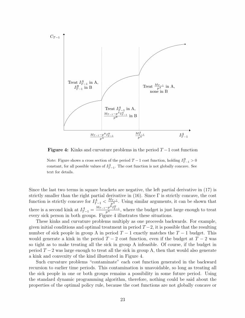
MAT−1pA

IAT−1

CT−1

MT−1−pBIBT−1pA

Treat IAT−1 in A,IBT−1 in B

Treat IAT−1 in A,MT−1−pAIAT−1

pBin B

Treat MT−1pA

in A,none in B

Figure 4: Kinks and curvature problems in the period T−1 cost function

Note: Figure shows a cross section of the period T − 1 cost function, holding IBT−1 > 0constant, for all possible values of IAT−1. The cost function is not globally concave. Seetext for details.

Since the last two terms in square brackets are negative, the left partial derivative in (17) isstrictly smaller than the right partial derivative in (16). Since Γ is strictly concave, the costfunction is strictly concave for IAT−1 <

MT−1

pA . Using similar arguments, it can be shown that

there is a second kink at IAT−1 =MT−1−pBIB

T−1

pA , where the budget is just large enough to treatevery sick person in both groups. Figure 4 illustrates these situations.

These kinks and curvature problems multiply as one proceeds backwards. For example,given initial conditions and optimal treatment in period T−2, it is possible that the resultingnumber of sick people in group A in period T − 1 exactly matches the T − 1 budget. Thiswould generate a kink in the period T − 2 cost function, even if the budget at T − 2 wasso tight as to make treating all the sick in group A infeasible. Of course, if the budget inperiod T −2 was large enough to treat all the sick in group A, then that would also generatea kink and convexity of the kind illustrated in Figure 4.

Such curvature problems “contaminate” each cost function generated in the backwardrecursion to earlier time periods. This contamination is unavoidable, so long as treating allthe sick people in one or both groups remains a possibility in some future period. Usingthe standard dynamic programming algorithm, therefore, nothing could be said about theproperties of the optimal policy rule, because the cost functions are not globally concave or

23

convex. By making assumption 1 and altering the dynamic programming algorithm to takeadvantage of that assumption, we established that the cost function is always concave overthe relevant range of infection levels. This permitted us to conclude that in each period thehealth authority should focus on the sick of a single group.

24