Embed Size (px)
Citation preview

Andean Highway Pass Program
Financial and Economic
Appraisal
prepared for
Inter-American Development Bank
As a subcontract to
Louis Berger International, Inc.
Final Report June 12, 1998

Table of Contents
Chapter Topics Page 1 Introduction 4-5 2 Analytical Framework 6-9 2.1 Program Description and Strategic Options 6 2.2 Analytical Approach 9 3 The Macroeconomic Environment 10-14 3.1 Introduction 10 3.2 Framework 11 3.3 Empirical Results of Macroeconomic Growth Forecasts 11 3.4 Trade Growth Forecasts and Trade Distribution 12 3.5 Role of the Passes 14 4 Economic Benefit and Cost Flows 15-21 4.1 Identification of Costs and Benefits 15 4.2 Economic Benefits from Cargo Traffic 15 4.3 Economic Benefits for Passengers 18 4.4 Other Economic Benefits 18 4.5 Economic Costs of Capital and Foreign Exchange 19 4.6 Economic Costs of Labor, Tradable, Non-Tradable Inputs 19 4.7 Economic Cost of Transportation 21 5 Economic Appraisal of Alternative Passes 22-31 5.1 Introduction and Methodology 22 5.2 Analysis of Individual Passes 23 5.3 Analysis of Combined Passes 24 5.4 Determination of the Recommended Investments 29 5.5 The Recommended Program of Investments 31 6 Distributional Impacts 32-36 6.1 Distribution by Country 32 6.2 Distribution by Sectors 34 7 Fiscal Impacts 37-38 7.1 Introduction 37 7.2 Methodology and Key Assumptions 37 7.3 Empirical Results 38 8 Sensitivity and Risk Analysis 39-45 8.1 Introduction 39 8.2 Methodology 39 8.3 Empirical Results 40 9 Conclusions 46-47
2

Appendices Page A The Macroeconomic Forecast 48-81 B Economic Benefits of Cargo Traffic 84-87 C The Economic Cost of Foreign Exchange 88-100 D The Economic Cost of Labor 101-105 E Economic Costs of Tradable and Non-Tradable Goods 106-108 F The Conversion Factors of Transportation Services 109-111
3

1 INTRODUCTION
Argentina and Chile share one of the longest borders in the world -- more than
5,000 km. Since the beginning of civilization, the Andes Mountains have restricted land
transportation between the two countries. The Andean Highway Pass Program is
designed to provide permanent crossings for trucks and passenger cars under all weather
conditions between cities in the two countries.
The Program is a pure public sector infrastructure investment. There are many
possibilities for passes between the two countries and the construction or improvement of
them should involve both governments. The main objectives of this report are to assess
the economic viability of investments in various passes and the associated fiscal
implications for the governments of Argentina and Chile, respectively.
There will be no conventional financial appraisal of the investments from the
private perspective, since no private ownership of the investment is involved in this
Program. Nevertheless, the technical designs and the engineering cost estimates should
provide important data for economic analysis of the public investments. Furthermore, the
forecasts of cargo and passenger traffic should form an important component of the
economic appraisal.
The economic appraisal evaluates the investment of individual passes and
combined passes from the viewpoint of the Argentinean and Chilean economy,
respectively, as well as of the southern Latin American region as a whole. It starts with
financial costs and develops a series of adjustments for the most important externalities to
reflect the economic costs and benefits for each of the two countries. The streams of
these net economic costs over the life of the investment project are then weighed against
a series of economic benefits generated by incremental vehicle traffic resulting from the
reduction in transportation costs and travel time. The results constitute the total
economic net benefits, from which a recommended program of investments will be
derived.
4

Sensitivity and risk analyses of the investment potential of the recommended
passes are also provided, demonstrating the expected effect of important variables.
The report is organized as follows: Section 2 presents the analytical approach and
framework of the public sector investment program. Section 3 discusses economic
growth and its relationship to trade flows among countries over the life of the project.
Details of economic costs and benefits are presented in Section 4. Section 5 presents
empirical results of the economic appraisal and the recommended program of
investments. Distributive benefits by country and sector of the economy are provided in
Section 6. Section 7 presents fiscal implications for the governments of Argentina and
Chile, respectively. Section 8 provides the outcome of the sensitivity and risk analyses
for key variables in the projects. Conclusions are summarized in the final section.
5

2 ANALYTICAL FRAMEWORK
The Andean High Pass Program will be evaluated as a pure public sector
infrastructure investment. Since each pass crosses the territory of Argentina to Chile, it is
considered a bi-national investment. Each investment may affect not only the economies
of Argentina and Chile, but also those of other countries, especially countries located in
the lower half of South America. Since the Program is a public sector investment, the focus of the analysis will be
on economic evaluation. The analysis is organized around the two major stakeholders in
the project: Argentinean residents and Chilean residents. Each pass is constructed jointly
by the Argentinean and Chilean governments, but the economic costs and benefits are
estimated separately for Argentina, Chile and the rest of the world.
2.1 Program Description and Strategic Options
There were 13 passes under initial consideration in the Andean Highway Pass
Program. As of the completion of this report, decisions on whether or not to proceed with
construction on several passes have been made. The Technical Group agreed not to
improve the Coihaique pass, while it has already begun construction of the Cardenal
Samore pass, which is expected to be fully paved by the end of 1998. Once completed,
the pass should serve both light and heavy vehicles throughout the year. Current capital
expenditures on the Cardenal Samore pass will not be included in the program, but are
considered part of the “do nothing” scenario under the evaluation.
The remaining 11 passes may all be paved. Some passes, such as the Sico, San
Francisco, Pircas Nigra and Huemules, may be coated with gravel rather than paved.
Capital investment for covering with gravel is less than for paving. The amount of annual
maintenance costs, however, may well be more for gravel than for paving.
In the initial analysis, all passes are assumed to be paved. In cases where
empirical results show paving to be economically unfeasible, alternative gravel roads will
be considered. The length of time and the expected investment costs for each pass,
expressed in 1998 prices, are provided for Argentina and Chile, in Table 2-1. The cost
6

estimates are for paved roads. One can calculate the capital expenditures per kilometer to
see whether one pass is more expensive than another.
It may be noted that there are no capital expenditures associated with the paving
of the Chilean side of the Cristo Redentor and Huemules passes. For the Cristo Redentor
pass, the Chilean side is already paved. The Huemules pass is entirely within Argentina.
It is of interest only to Argentina and all the expenditures would be incurred by the
Argentinean government.
Table 2-1 Length and Investment Cost of Passes
Name of Distance Capital Costs
Pass Argentina Chile Total Argentina Chile Total (km) (thousands of US dollars) Jama 255 156 441 50,816 54,000 104,816
Sico 266 217 483 59,078 59,241 118,319 San Francisco 199 260 459 36,522 45,355 81,877 Pricas Negras 186 200 386 73,136 59,000 132,136
Agua Negra 91 149 240 50,327 31,500 81,827 Cristo Redentor 134 66 200 42,091 0 42,091 Pehuenche 76 173 249 32,528 32,900 65,428 Pino Hachado 53 179 232 6,686 15,400 22,086 Huemules 134 46 180 37,708 0 37,708 Integración Austr 54 43 97 19,786 4,256 24,042 San Sebastián 13 161 174 3,319 42,665 45,984
The maintenance costs required for the passes depend upon several factors, such
as the type of pass, the height and curve of the pass, and the type of snow removal to be
used. Because paved road is considered first in the study, we present the annual
maintenance costs for paved road in Table 2-2. The costs include wages; salaries;
materials such as asphalt, gravel, cement, fuel, lubricants, and steel; rental of equipment,
and other.
7

Table 2-2 Annual Maintenance Costs of Each Pass
(thousands of 1998 US dollars)
Name of Pass Argentina Chile Total Jama 340 188 528
Sico 356 261 617 San Francisco 308 368 676 Pricas Negras 273 224 497
Agua Negra 269 417 687 Cristo Redentor 296 136 433 Pehuenche 156 317 473 Pino Hachado 88 276 364 Huemules 180 56 235 Integración Austr 93 59 151 San Sebastián 22 249 271
When each pass is considered, one must assess the substitution and
complementary effects of the particular investment on the traffic and on the economy. If
there is a substitution effect, then the incremental effect of the investment on the pass in
question should be less than its independent effect. Presumably, the pass competes with
existing passes, and the net incremental economic benefits should therefore be smaller
than if the pass were evaluated on its own.
To the contrary, if there is a complementary effect from improving the pass, the
incremental impact of the investment on traffic and on the economy should be greater
than if the impact of the pass is assessed independently.
Out of the 11 passes, five have been studied in depth by the technical group of the
Program and expected to be constructed sooner than the others. These passes - Jama,
Agua Negra, Cristo Redentor, Pehuenche, and Integracion Austral, will each be evaluated
for economic feasibility, and a determination will be made on when to begin
construction.
The remaining six passes will be considered in the future, pending the evaluation
of analytical results.
8

2.2 Analytical Approach
Since no toll will be charged for the newly paved passes, and there will be no
financial revenue from the investments, there will be no traditional financial appraisal of
this program. However, there will be fiscal implications of this public sector investment
for the governments of Argentina and Chile.
The economic appraisal will assess the program in terms of its economic impact.
Since each pass represents a joint investment by Argentina and Chile, the net economic
benefits should accrue principally to the residents of Argentina and Chile, but also to the
rest of southern Latin America. While the benefits to individual countries are an
important concern, the total benefit to the region should be the prime consideration for
investment decision-making.
In this analysis, each pass will first be assessed independently in economic terms.
The individual assessments will then be followed by an evaluation of the combined
passes and recommended investments for the Program.
9

3 The Macroeconomic Environment
3.1 Introduction
The key determinants for the economic appraisal of the Andean Pass Program are
the volumes of freight and passenger traffic and the costs of investment. Among the
important variables determining the level of traffic that is expected to benefit from the
passes are current levels of income, trade flows between Argentina, Chile and other
countries, and the future growth path of these variables. Due to the time value of money,
the levels of income, trade flows and their growth in the near future should have a much
bigger impact on the demand for highway services and the feasibility of the investment
than prospective income growth rates 10 to 20 years after the pass is improved.
Making a precise long-term macroeconomic forecast for different countries is
difficult and possibly unrealistic, because many unknown factors influence the
performance of the economy in question. This is especially true when the countries’
formerly highly protected economies are in the process of opening up to international
competition. In this situation, when the governments are launching major economic
policy initiatives, many factors can change prospects for economic growth rather
suddenly.
Given the history of volatile economic policies in these countries over the past 50
years, it is difficult to forecast with any degree of certainty future economic policies for
the region and the likely economic outcomes from these policies. Our model is designed
to address the forecasts and beliefs of the decision-makers which will be factors in
determining the future of the investment.
For the highway project, forecasts of the real gross domestic product for
Argentina, Chile, and other members of Mercosur may not be as important as the forecast
of trade flows among these countries. The growth in trade flows in the short run should
be highly dependent on both trade and real exchange rate policies. Over the longer run,
they should depend on the level of integration of the respective countries’ economies,
which reflects an equilibrium situation for them.
10

For an economic analysis, one needs to develop a series of scenarios in order to
understand the nature of economic outcomes of the project and to communicate these
interrelationships. To do this, one needs to develop forecasts of GDP that will serve as
the basis for the forecasts of demand for the services of the passes. In the analysis that
follows, the likely range of growth rates in these countries has been based on the
fundamental determinants of economic growth in the countries, tempered by the short-
term policy constraints they currently face.
3.2 Framework
Our analytical framework is based on the hypothesis that an increase in GDP can
be measured by the sum of the increase in factor incomes – real wage and capital income
– and a residual item that can be categorized as the reduction in real costs, or an increase
in factor productivity.1
To make a forecast of the economic growth rate of a country for the future, one
must obtain values for each of the above three components. These values must reflect not
only the past experiences of the country in question, but also its economic expectations
for the future. As one can expect, a reduction in real costs may be influenced by many
factors other than productivity. For example, major economic reforms and political
instability are not represented in the first two components, but they are certain to have an
effect on the economic growth of the country.
3.3 Empirical Results of Macroeconomic Growth Forecasts
In Appendix A, a detailed analytical framework is developed, and an empirical
estimation is made for construction of the bands of low, most likely and high growth rates
for Argentina and Chile. It is our conclusion that for Argentina, the range of growth rates
that fits these bands is 3, 4 and 5 percent, respectively. In the case of Chile, the growth
rates are expected to be higher. The corresponding ranges are 3.5, 5.0 and 6.5 percent,
respectively. For the purpose of this analysis, we assume that the annual growth rates for
Brazil, Paraguay and Bolivia will range from 3 to 5 percent.
11

The GDP growth forecasts, as well as the growth rates for the past several years,
are summarized in Table 3-1.
Table 3-1
Annual Growth Rates of Real GDP
Year Argentina Chile High Base Low High Base LowActual
1990 0.06 1991 8.90 7.30
1992 8.65 11.00 1993 6.03 6.30 1994 7.42 4.20 1995 -4.40 8.50 1996 4.25 7.20 Estimated*
1997 7.50 6.00
Forecast 1998 5.00 4.00 3.00 6.50 5.00 3.50 1999 5.00 4.00 3.00 6.50 5.00 3.50 2000 5.00 4.00 3.00 6.50 5.00 3.50 2010 5.00 4.00 3.00 6.50 5.00 3.50 2020 5.00 4.00 3.00 6.50 5.00 3.50
3.4 Trade Growth Forecasts and Trade Distribution
Trade is closely related to economic growth rates. Over the past two decades,
Chile has developed a relatively open economy. Several recent studies show us that the
aggregate trade elasticities relative GDP range from 1.01 to 1.82 for exports and from
1.07 to 1.74 for imports2, respectively. For the purpose of this study, we are assuming
that the trade elasticities for exports and imports are 1.75 over the next 10 years and 1.50
in the remaining years of the Program, for both Argentina and Chile.
At present, Argentina engages in a significant amount of trade with the rest of the
Mercosur members and the European countries. We expect there to be a slight shift in
terms of percentage distributions of trade to Asia and members of North American Free
1 Details can be found in Arnold C. Harberger, “Reflections on Economic Growth in Asia and the Pacific”, Journal of Asian
Economics, (1996). 2 See Appendix A, “The Macroeconomic Environment of the Andean Highway Passes Program”, Table 3.
12

Trade Agreement (NAFTA). The forecasts of such trade distribution flows between
Argentina and other countries or regions are displayed in Table 3.2.
Table 3.2
Argentinean Trade Distribution by Region (percentage)
Rest of Rest of South Rest of NAFTA Chile Mercosur America Europe Asia World
Exports 1994 12.6 6.0 29.1 5.3 25.2 8.4 13.4 1996 9.6 7.4 33.3 4.9 19.5 10.0 15.1 2010 14.0 8.0 34.0 4.0 19.0 12.0 9.0 2010 14.0 8.0 34.0 4.0 19.0 12.0 9.0 Imports 1994 23.3 3.6 22.5 1.6 31.6 10.3 7.1 1996 23.4 2.4 24.5 1.9 30.4 9.7 7.7 2010 24.0 4.0 26.0 1.0 29.0 11.0 5.0 2010 24.0 4.0 26.0 1.0 29.0 11.0 5.0
Chile’s major trading partners have been the countries of Europe and NAFTA.
Trade among these countries is expected to continue to grow. In the meantime, trade
between Chile and members of the Mercosur region is expected to be enhanced at the
expense of the rest of South America. Chilean trade with other countries and regions are
shown in Table 3.3.
Table 3.3
Chilean Trade Distribution by Region (percentage)
Rest of Rest of South Rest of NAFTA Argentina Mercosur America Europe Asia World
Exports 1994 19.5 5.4 6.1 6.6 24.4 15.8 22.1 1996 18.5 4.6 6.9 6.6 24.6 17.0 21.8 2010 20.0 6.0 7.0 6.0 24.0 17.0 20.0 2010 20.0 6.0 7.0 6.0 24.0 17.0 20.0
13

Rest of Rest of South Rest of NAFTA Argentina Mercosur America Europe Asia World
Imports 1994 27.4 8.3 9.5 4.9 22.9 9.6 17.4 1996 31.4 9.4 6.8 5.3 21.7 10.5 14.9 2010 31.0 10.0 9.0 5.0 21.0 12.0 12.0 2010 31.0 10.0 9.0 5.0 21.0 12.0 12.0
3.5 Role of the Passes
As mentioned earlier, the demand for freight traffic is expected to be determined
by the magnitude of trade between Argentina, Chile and other countries. Once the passes
are improved, the relationship between Argentina, Chile and other members of the
Mercosur region should strengthened.
By the same token, but to a lesser extent, the improvement of passes should lower
transportation costs and enable passengers to have access to roads between Argentina and
Chile.
14

4 Economic Benefit and Cost s
4.1 Identification of Costs and Benefits
The measurement of economic benefits and costs is typically based on
information developed in the financial analysis from the total investment viewpoint.
However, there will not be a traditional financial analysis in this Program, because no
financial revenues will be generated by this public sector infrastructure investment.
In the economic appraisal, all the prices of goods and services used in the project
are measured in economic terms. Conversion factors, used to calculate economic prices
as a function of their financial values, are calculated for Argentina and Chile,
respectively. The economic price of foreign exchange, for example, differs in each
country from its market value because of a variety of distortions associated with the
markets for traded goods.
In the Andean highway Passes program, primary sources of economic benefit are
generated by cargo and passenger traffic. Secondary benefits may arise due to taxes and
other distortions in the markets affected by the construction or maintenance of the passes,
but these should be small relative to the direct benefits arising from the traffic flow.
4.2 Economic Benefits from Cargo Traffic
The economic benefits from the cargo traffic on the pass are generated by savings
in transportation costs and logistic costs, including loading/unloading costs and waiting
time.
The cargo demand model is developed in such a way that receivers of freight
minimize the total delivered cost expressed per unit of product shipped. The model
provides calculations for a sample of actual shipments and picks the mode and route to
minimize the total landed cost. The transportation mode or route should change when the
cost of another mode or route becomes cheaper.
In the model, the most important variables for determining the total 15

transportation and logistics costs are distance traveled, waiting time to cross the border
(i.e., customs operations), fuel, labor and harbor loading/unloading (if any). It is the cost-
minimizing features of the model that determine the volume of traffic that will be
diverted and generated by improvement of the passes. The growth in traffic over time is
determined by the growth in international trade in the region.
Demand and total transportation cost savings have been determined in another
module of this study. The important question in this regard is whether the exporting or
importing country is receiving the economic benefits of cargo traffic across the passes.
When the commodity is internationally traded with third countries by the importing
country, the cost savings from the reduction in transportation costs should accrue to the
producers in the exporting country, because the goods can continue to be sold in the
importing country at prices based on world prices. A detailed explanation of these
fundamental relationships is presented in Appendix B.
In terms of measurement, the benefits for diverted traffic are equal to the
reduction in transportation costs times the volume of diverted traffic. For induced and
generated traffic, the benefits are equal to one half of the transportation cost savings
mulplitied by the traffic volume.
If goods are not internationally traded but mainly imported from the exporting
country in the Mercosur region, the benefits resulting from transportation cost reductions
should be shared by producers of the exporting country and consumers of the importing
country, depending upon the magnitude of demand elasticity for imports and supply
elasticity for exports. The share of benefits received by importing country (λ) can be
measured by:
λ = εsx/[εs
x - ηdx]
where εsx refers to the elasticity of supply of exports from the exporting country and ηd
x
refers to the elasticity of demand for the same commodity from the perspective of the
importing country. (See Appendix B.)
16

Appendix B also reveals that the share of benefits received by the importing
country ranges from 37% to 81% of the total. We can reasonably assume that benefits
resulting from savings in transportation costs should be shared equally by importing and
exporting countries. However, for the purpose of this analysis, all commodities imported
by Argentina and Chile are considered to be internationally traded.
In terms of measurement, the benefits for diverted traffic are measured by the
amount of savings in transportation costs times the traffic. For induced and generated
traffic, the benefits are estimated by multiplying one half of the transportation cost
reduction by the incremental traffic.
Having laid out the basic principles for measuring economic benefits, some
shipments of cargo should receive special attention:
• An incremental shipment from Asia or NAFTA to Argentina via the passes.
Because of transportation cost reductions, cost savings should accrue to
consumers in Argentina, not to producers in the exporting countries of Asia or
NAFTA. This is due to the fact that the exporting country can continue to sell
products at prices based on international prices and that, the prices of goods sold
in the importing country could be lowered to commensurate with the reduction in
transportation costs. Therefore, consumers in Chile should not receive benefits
directly in terms of lower-priced imports, but economic activities in the
transportation and port sector should increase.
• An incremental shipment from Asia or NAFTA to Paraguay, Bolivia or Brazil via
the passes. By the principle outlined above, benefits should accrue to consumers
in the importing countries.
• An incremental shipment originating in Argentina, Paraguay, Bolivia or Brazil
going to Asia or NAFTA. The benefits should accrue to producers in the
exporting countries.
17• A shipment originating and terminating in the same country (either

Argentina or Chile): Although the benefits resulting from savings in
transportation costs should ideally be shared equally by the importing and
exporting regions, in practice they will probably be spread unevenly among the
various countries. This will be true for some of the improved passes.
4.3 Economic Benefits for Passengers
At the present time, passengers between Argentina and Chile travel primarily by
car or plane. The economic benefits of diverted and induced passenger traffic are
measured by savings in vehicle operating costs and in time savings gained through use of
the improved passes, as well as by the value of any taxes or distortions associated with
vehicle and time costs incurred to use the passes.
In addition, lost or gained tax revenue associated with foregone operating costs
(because of the reduction in activity of the alternative modes due to the quantity of traffic
diverted to the pass) is accounted for in the analysis.
4.4 Other Economic Benefits
In addition to the economic benefits for cargo and passenger traffic, one has to
identify the project’s externalities by subtracting the financial costs from the real
economic costs. The analysis considers the benefits that Argentina and Chile should
receive from the sale of goods and services to the project in exchange for resources
generated by producing those goods and services, including the benefits and costs of
using foreign exchange, labor and other business inputs that can be expressed in
conversion factors.
In the economic analysis, the benefits and costs are expressed in U.S. dollars. The
net present value (NPV) of the net economic benefits of the project will be the criteria
used for decision-making and ranking of the investment potential of the various passes.
To calculate the NPV of the economic benefits and costs of the highway project, the
respective economic costs of capital for Argentina and Chile are employed. These
18

parameters are used to discount a series of economic benefits and costs over the life of
the project.
4.5 Economic Costs of Capital and Foreign Exchange
The economic cost of capital is determined as a weighted average of the foregone
consumption, the gross-of-tax returns on domestic investment, and the marginal costs of
foreign borrowing. This parameter is used to discount the net economic benefit stream
arising from investment in the passes in order to derive the economic net present value
for each country. The economic cost of capital is assumed to be 12 percent real for
Argentina and Chile.3
The economic cost of foreign exchange is calculated in Appendix C. The
economic cost of foreign exchange in 1998 to date is 10.88% higher than the official
exchange rate in Argentina and 15% higher than the rate Chile. This foreign exchange
premium is due in part to the impact of net import tariffs and value added taxes. The
premium for Argentina should slightly decline over time until 2001 because of the
Mercosur Treaty and the global trade liberalization. In the case of Chile, the foreign
exchange premium should depend upon future trade and tax policies. Free trade with
either Mercosur or NAFTA calls for a reduction in import tariffs and should lower the
foreign exchange premium. However, in order to have revenue-neutrality in the public
sector budget, the reduction of import duties should lead to an increase in indirect taxes
levied on domestic consumption of goods and services, thereby raising the foreign
exchange premium. Therefore, the foreign exchange premium used in the evaluation of
this Program is approximately 15%.
4.6 Economic Costs of Labor, Tradable and Non-Tradable Inputs
Investment and operating cost components consist of individual item costs such as
labor, tradable machinery, equipment and material, and non-tradable goods. The
conversion factors for these individual items must be calculated, so that their financial
193 From the Inter-American Development Bank in the terms of the contract.
costs can be translated to reflect the economic prices of business inputs and so that the
associated distortions can be quantified.
Economic Cost of Labor
The economic cost of labor for the project varies by type of skill required and by
type of labor market. There are three skill levels of construction worker required for the
project during the two to three years of construction. Similarly, there are three types of
operating worker required over the life of the operating/maintenance phase.
There are competitive labor markets in Argentina and Chile. This analysis uses
the private price of labor to induce people to work for a project as the fundamental
determinant of the economic cost of labor.4 It is then adjusted for any gain or loss in
taxes and social security contributions paid to the government, exclusive of any direct
pension benefits gained by workers upon their retirement.
The assumptions and calculation of the economic cost of labor can be found in
Appendix D. The results indicate that the economic cost of labor is approximately 96%
of the wage bill for professionals, 91% for skilled and 90% for unskilled workers in
Argentina and Chile. In other words, the net labor externalities from employment in this
program would be 4% of the wages for professionals, 9% for skilled and 10% for
unskilled workers.
Economic Cost of Tradable Inputs
During the construction period of the highway project, all machinery and
equipment or rented property used in the project are considered tradable inputs. Thus, the
financial price of each input should be adjusted for the foreign exchange premium. For
example, the foreign exchange premium for Chile in 1998 was estimated to be 15%. The
20

conversion factor for tradable inputs is equivalent to 0.878, because imports in Chile are
all subject to an 11% tariff, an 18% value-added tax, and a 15% foreign exchange
premium. Thus, the economic price for tradable inputs such as steel is 12.2% lower than
the financial cost.
All of the conversion factors for tradable inputs used in the operational period of
the highway passes are calculated for both Argentina and Chile. These items including
fuels, lubricants and tires are related mainly to vehicle maintenance costs. They are
adjusted for the foreign exchange premium, tariff and value added tax. For example,
gasoline in Argentina is subject to a 70% excise tax and 21% of the VAT rate. Its
conversion factor for 1998 is equal to 0.5390 [=(1/((1.7)*(1.21)))*(1.1088)]. For diesel
fuel, it is 0.689. For Chile, the conversion factor for gasoline is estimated at 0.6968 and
for diesel, at 0.6124.
Details can be found in Appendix E.
Economic Cost of Non-Tradable Inputs
In the case of non-tradable goods, the economic cost is estimated as a weighted
average of the value of the resources used in the production of additional supply and the
value of consumption foregone by the existing demand. For the purpose of this study, we
assume an equal weight for demand and supply. For example, the conversion factor for
Portland cement would be 0.7958 for Argentina and 0.8584 for Chile.
4.7 Economic Cost of Transportation Services
Transportation services are major inputs for the highway project. The calculation
of conversion factors for passenger cars, passenger buses and truck transport are based on
a detailed breakdown of vehicle operating financial costs per 1,000 vehicle km. They are
0.8896, 0.8509, and 0.8845, respectively, for Argentina. The corresponding figures for
Chile are 0.9128, 0.9001, and 0.8679, respectively. (See Appendix F.)
21
4 See A. C. Harberger, “On the Social Opportunity Cost of Labor”, in Project Evaluation: Collected Papers, (Chicago: University of
Chicago Press, 1972); and A. C. Harberger, “The Social Opportunity Cost of Labour, Problems of Concept and Measurement as

5 Economic Appraisal of Alternative Passes
5.1 Introduction and Methodology
The economic appraisal of an investment focuses on the economic costs and
benefits of the investment for participating countries. To achieve this objective, the
financial costs incurred in the project have to be converted into economic costs, which
will affect the economy of the countries. In addition, there should be an accounting of
the net economic benefits generated specifically from changes in the demand for cargo
and passenger traffic.
As previously discussed, the highway project is expected to have a direct impact
on the economy of Argentina and Chile and an indirect effect on Brazil, Paraguay,
Bolivia and Uruguay. In this section, the economic appraisal will focus on the total net
economic benefits of a specific investment in the region rather than on the benefits
accruing to the individual economies of Argentina and Chile. The distributive benefits of
the investment will be covered in the next section.
The economic principles developed in the field of welfare economics are utilized
extensively in this highway project. In the economic analysis, all prices are measured in
economic terms. Conversion factors, used to calculate economic prices as a function of
their financial values, were calculated in Section 4 for Argentina and Chile, respectively.
Resources used over the life of the project are all expressed in economic prices. In
addition, the economic benefits generated from changes in cargo and passenger traffic as
a result of savings in transportation are taken into account in the overall economic
appraisal of the specific investments in question.
The present value of the total net economic benefits of the investment will be the
principal criterion for the determination of the recommended investments in this
Program.
Seen from a Canadian Perspective”, paper prepared for the Task Force on Labour Market Development, the Government of
22

5.2 Analysis of Individual Passes
As mentioned in Section 2, the Cardenal Samoré pass is currently being paved on
the Argentinean side and will be fully paved by the end of 1998. The Chilean
government plans to pave access to the Pass on the Chilean side in order to complement
the work being undertaken on the Argentinean side. Since these works are all underway,
the capital expenditures for this pass are not considered part of the program of
investments. In other words, this pass is assumed to have been improved and is
considered as part of the “do nothing” scenario under the evaluation of this Program.
First, the capital investments of each pass are evaluated individually. The results,
presented in Table 5.1, show the combined economic benefits for Argentina, Chile and all
other countries of the investment from each pass individually. This is the incremental
economic benefit of each pass in addition to the improvement of the Cardenal Samoré
pass.
Construction on all passes is assumed to begin in 1999. The results are based on
the most likely economic growth scenario and a modest trade elasticity. That is, the
annual GDP growth rates are 5% for Chile and 4% for Argentina and the rest of southern
Latin America over the life of the project. The trade elasticity is 1.5 for exports and
imports for both Argentina and Chile.
Table 5.1
The Economic NPV of Each Pass For the Base Case Scenario
(thousands of 1998 US dollars)
Jama 86,678 Sico 80,571 San Francisco (589) Pircas Negras 8,905 Agua Negra 94,756 Cristo Redentor 55,420 Pehuenche 200,967 Pino Hachado 142,692 Huemules 2,219 Integración Austral 10,379 San Sebastian 15,545
23
Canada, (July 1981).

24
The ranking of individual passes in terms of combined economic benefits is:
Pehuenche, Pino Hachado, Agua Negra, Jama, Sico, Cristo Redentor, San Sebastián,
Integración Austral, Pircas Negras, Huemules and San Francisco. With the exception of
San Francisco, all the passes generate a positive net present value individually. This
means that the improvement of each pass (other than San Francisco), if evaluated in
isolation, would result in economic benefits.
Having said this, one should be aware that the above assessment may not be
totally accurate, because no substitute or complementary effects have been taken into
account. In other words, the ranking presented above may eventually be altered when
subsequent passes are considered.
5.3 Analysis of Combined Passes
Consideration of the substitute and complementary effects is vital when
subsequent passes are assessed for possible implementation. For example, the Pehuenche
and Pino Hachado passes were considered the best two passes individually, but if these
passes are improved at the same time, the total benefits (US$283,692 thousand) are
smaller than the sum of each individual passes (US$ 200,967 thousand plus US$142,692
thousand). This implies that these two passes are to some extent competitive pairs.
Another extreme example is that of Jama and Sico. Their net economic benefits
would be US$86,678 and US$80,571, respectively, if they were constructed
independently. However, if these two passes were improved simultaneously, the total net
benefits would be US$26,506, which is less than either pass by itself. This results from
two factors. First, there would be a marginal increase in traffic expected if both passes
were improved and opened, compared to opening one pass with more traffic. For
example, the total annual volume of trucks crossing Jama and Sico would be only slightly
greater than that of either Jama or Sico alone (i.e., 51,830 vs. 49,640 or 48,910 vehicles).
Similarly, the increase in the annual volume of passenger auto traffic would also be
marginal (i.e., 100,740 vs. 98,915 or 98,550 vehicles). This can be seen from the daily
traffic shown in Table 5.2 for the most likely economic growth scenario in

Table 5.2 Estimates of Total Demand for Vehicle Traffic Through Various Passes in 2010
-- With the Improvement of the Jama and Sico Passes -- (daily traffic)
Improvement of Jama Improvement of Sico Improvement of Jama and Sico
Trucks Buses Cars Total Trucks Buses Cars Total Trucks Buses Cars Total Jama 131 8 270 408 20 - 1 21 76 4 148 228 Sico 5 - 1 6 114 8 269 391 66 4 128 198 San Francisco - - 1 1 - - 1 1 - - 1 1 Picas Negras - - - - - - - - - - - - Agua Negra - - 14 14 - - 14 14 - - 14 14 Cristo Redentor 795 218 1,047 2,059 795 218 1,047 2,060 789 217 1,044 2,051 Rehuenche - - 2 2 - - 2 2 - - 2 2 Pino Hachado 28 7 59 94 28 7 59 94 28 7 59 94 Cardenal Samoré 79 39 525 643 79 39 525 643 79 39 525 643 Coihaique - 1 69 70 - 1 69 70 - 1 69 70 Huemules 18 1 50 69 18 1 50 69 18 1 50 69 Integracion Austral 119 23 387 529 119 23 387 529 119 23 387 529 San Sebastian 77 18 158 252 77 18 158 252 77 18 158 252 Total 1,251 318 2,581 4,147 1,249 315 2,582 4,145 1,251 314 2,584 4,150


the year 2010. Similar results are obtained for other years. Second, with virtually no
increase in traffic when the second pass is improved, all resources spent on the second
pass would be redundant and the total combined net economic benefits would decrease,
rather than increase.
Alternative pairs of competing passes are examined using the most likely
economic growth scenario and the year 1999 as the first year of construction. Included
are Jama vs. Sico, Pircas Nigras vs. San Francisco, Pehuenche vs. Cristo Redentor and
Pehuenche vs. Pico Hachado. There are considered competing because the total net
economic benefits resulting from the paving of the two passes are forecast to be less than
the sum of the net economic benefits from the two independent passes. These pairs have
varying degrees of competition. Some pairs are substantially independent, such as
Pehuenche and Cristo Redentor, and Pehuenche and Pino Hachado. The summary results
can be found in Table 5.3.
Table 5.3
The Economic NPV of the Competitive Passes For the Base Case Scenario
(thousands of 1998 US dollars)
Jama 86,678 Sico 80,571 Jama and Sico 26,506 Pircas Negras 8,905 San Francisco (589) Pircas Negras and San Francisco (43,983) Pehuenche 200,967 Cristo Redentor 55,420 Pehuenche and Cristo Redentor 190,036 Pehuenche 200,967 Pino Hachado 142,692 Pehuenche and Pino Hachado 283,692
To the contrary, some pairs of passes may be complementary in the sense that the
total net economic benefits resulting from the paving of the two passes should be
virtually the same or greater than the sum of the net economic benefits from the two
independent passes. The passes which fall into this category include the pairs of

Pehuenche vs. Agua Negra, Pehuenche vs. Jama, Pehuenche vs. Sico, Agua Negra vs.
Cristo Redentor, and Integración Austral vs. San Sebastián. Table 5.4 presents the net
economic benefits of these pairs, using the most likely economic growth scenario and the
year 1999 as the first year of construction.
Examining these pairs more closely, one discovers that most are geographically
distant, serving different markets. The exceptions are the pairs of Agua Negras vs. Cristo
Redentor and Integración Austral vs. San Sebastián. The former pair would serve the
highest levels of traffic between the central regions of Argentina and Chile. The latter
pair is basically additive, because one has to travel both passes in order to reach Tierra
del Fuego from Argentina.
Table 5.4 The Economic NPV of the Complementary Passes
For the Base Case Scenario (thousands of 1998 US dollars)
Pehuenche 200,967 Agua Negra 94,756 Pehuenche and Agua Negra 291,729 Pehuenche 200,967 Jama 86,678 Pehuenche and Jama 288,142 Pehuenche 200,967 Sico 80,571 Pehuenche and Sico 281,971 Agua Negra 94,756 Cristo Redentor 55,420 Agua Negra and Cristo Redentor 145,108 Integración Austral 10,379 San Sebastián 15,545 Integración Austral and San Sebastián 25,924
Other pairs are all independent of each other. The total net economic benefits
resulting from improvements to these pairs of passes are more or less additive compared
to the independent improvement of each pass.
28

5.4 Determination of the Recommended Investments
Argentina and Chile share a border of more than 5,000km, one of the longest in
the world. Because of the Andes Mountains, land transportation between the two
countries is limited. Strategically, an improvement of the northern, central and southern
blocks of passes could be mutually beneficial, because each block of passes serves
independent markets. Therefore, it would be practical to examine the economic impact
of the three blocks in isolation along with the above findings.
In each block, one should be mindful of the complementary pairs of passes
presented in the previous section. As indicated previously, the northern block pair of
Jama and Sico are competitive, serving the same markets, and passing through the same
harbor of Antofagasta. The improvement of Jama would result in greater incremental
economic benefits than the improvement of Sico and is therefore the best choice for
development. It should be noted that adding the Sico pass would result in a decrease in
the net economic benefits, because of the marginal increase in traffic.
In the central block, there are more passes to be considered, because of the
significant existing traffic and expected large future increase in traffic between Argentina
and Chile. Using the analytical results shown in the previous section, Pehuenche and
Cristo Redentor are good selections for improvement. This is reasonable because the
Cristo Redentor pass has already been paved on the Chilean side, and there is a
considerable volume of existing traffic. The construction of the Pehuenche pass should
divert some traffic from the Cristo Redentor pass because of its lower vehicle operating
costs and avoidance of interruptions caused by snow avalanches. The alignment of these
two passes would serve the highest levels of traffic between these two countries, resulting
in the most incremental economic net benefit of the investments.
The next pass to be improved in the central block might be either Pino Hachado
or Agua Negra. The rationale for improving Pino Hachado, on the one hand, reflects its
geographic independence from Cristo Redentor and on the other hand, its competition
with the Pehuenche pass, as pointed out in the previous section.
29

Table 5.6 Total Economic NPV of the Passes in the Central Block
For the Base Case Scenario (thousands of 1998 US dollars)
Pehuenche 200,967 Cristo Redentor 55,420 Pehuenche and Cristo Redentor 190,036 Pehuenche, Cristo Redentor and Agua Negra 281,683
The Agua Negra pass is by and large independent of the Pehuenche and Cristo
Redentor passes. The incremental economic net benefits to be gained by adding the
Agua Negra pass to the Pehuenche and Cristo Redentor passes should be greater than the
benefits of adding the Pino Hachado pass. Therefore, the Agua Negra pass should be
selected for paving prior to the Pino Hachado pass.
Next, consider the Pircas Negras and San Francisco passes. The incremental
benefits of adding either pass would be negative, especially San Francisco, which would
be expected to generate a negative return if improved independently. The alternative is to
improve the highway with gravel instead of paving. Nevertheless, the results still appear
to be unfeasible economically, even though the amount of total capital costs would
decline, because a gravel road would substantially reduce the volume of traffic compared
to a paved road.
Turning to the southern block, the choices are Integración Austral, San Sebastián,
and Huemules. Improving the Huemules pass should generate a marginal positive
economic benefit at the net present value of US$2.22 million over the life of the project,
since the traffic is mostly local within Chile, and its volumes would not be very large.
Nevertheless, the pass should permit the connection between Comodoro Revadavia in
Argentina and Puerto Chacabuco in Chile.
A comparison of the Integración Austral and San Sebastián passes indicates that
improving of the San Sebastian pass should generate a greater net benefit than improving
Integración Austral (i.e., US$15.5 million versus US$10.4 million). As indicated earlier,
these two passes are independent, and a passenger would need to travel both passes to
reach Tierra del Fuego from Argentina. As the Integración Austral pass was designed
30
well in advance of the San Sebastián pass, Integración Austral should be the first selected
for improvements in the southern block. The sequence of the highway investment in the
southern block should be Integración Austral, San Sebastián, and Huemules.
5.5 The Recommended Program of Investments
The above empirical results suggest that the passes with the most economic
benefits would include Jama in the north, Pehuenche, Cristo Redentor and Agua Negra in
the center, and Integracion Austral in the south. These five passes should be the first
paved, not only because they would generate the most economic net benefits but also
because they are substantially advanced in the design process. If these five passes are
constructed in 1999, the total economic net benefits could total approximately US$360.2
million in 1998 prices.
The subsequent paving in the Pino Hachado, San Sebastián and Huemules would
generate further positive net economic benefits in the region. Assuming that these three
passes are also improved beginning in 1999, the additional economic benefits would be
about US$101 million in 1998 prices.
In the case of the Sico, San Francisco and Pircas Negra passes, their paving would
produce a negative economic benefit. This is because the Sico pass is almost completely
competitive with the Jama pass, and the San Francisco pass is competitive with the Pircas
Negra pass. Therefore, they are not recommended for upgrading in 1999. Even if they
were covered with gravel instead of paved, the smaller amount of capital investment
necessary would still not be enough to generate a positive return, because of insufficient
volumes of traffic.
31

6 Distributional Impacts
The impacts presented so far are for the total net economic benefits to the region
as a whole. All passes cross the territories of Argentina and Chile, leading to other parts
of southern Latin America, including Brazil, Uruguay, and Bolivia. Each of them is
expected to have an impact on not only the economies of Argentina and Chile, but also
on other countries in southern Latin America as well. The investments should have an
impact on different sectors of the economy as well. This section of the report assesses
the impact of the recommended program of investments by country and by sector.
An analysis will be carried out for those passes, which are expected to produce a
positive net economic benefit for the region. We will present results for the first five
recommended passes, - Jama, Cristo Redentor, Pehuenche, Agua Negra, and Integración
Austral, - as a group. For the entire Program, we will also present results for all eight
passes as a whole, because the three additional passes, Pino Hachado, San Sebastián and
Huemules, should generate a positive net benefit.
For simplicity, we will present only results based on the most likely economic
growth scenario, starting in 1999.
6.1 Distribution by Countries
Most highway travelers in Argentina, Chile and other Latin American countries
are expected to choose the new passes over other highway routes. Changes from
alternative mode of transportation are not expected and are, therefore ignored for the
purpose of this analysis. The direct benefits for the passenger traffic, autos and buses
should reflect not only savings in traveling time and vehicle operating costs but also
improvements in reliability. All the benefits should be attributed to the passengers’
country of origin.
For cargo traffic, the improved passes should lower transportation and logistics
costs. Because of the competitive market in the international transportation sector and
because of international tradable goods, the exporting country should be able to sell more
32

goods to the importing country. Consequently, producers in the exporting country should
expand. Their operations for diverted traffic, benefits are calculated by multiplying the
reduction in transportation costs by the volume of diverted traffic. For induced and
generated traffic, the benefits are measured by multiplying one-half of the savings in
transportation costs by the volume of traffic.
As explained in the methodology section, for goods shipped from Asia or
NAFTA, benefits should accrue to consumers in the importing countries, because the
exported goods are expected to be sold at established international prices by the exporting
country.
For passenger traffic, all the benefits from the transportation cost savings accrue
to the travelers’ country of origin.
The above economic net benefits should be offset by the economic costs of
resources used for the project. These economic costs are measured in terms of economic
prices of capital goods and operating goods and services used in Argentina and Chile,
respectively. The conversion factors derived in the previous section for the economic
costs of labor, tradable and non-tradable business inputs, will be used to translate
financial costs into economic costs.
The streams of the above economic benefits and costs over the life of the project
should then be discounted by the economic cost of capital in the respective countries.
The economic cost of capital is assumed to be 12% real for both Argentina and Chile.
The economic net benefits for the two sets of recommended programs of
investments are presented in Table 6.1. These results are again based on the most likely
economic growth scenario, starting in 1999.
33

Table 6.1
The Economic NPV of Various Passes by Country For the Base Case Scenario
(thousands of 1998 US dollars)
Country Five Passes Eight Passes
Argentina 248,439 320,422 Chile 104,472 133,709 Rest of the World 7,295 7,297 Total 360,206 461,428
It is interesting to note that about 69% of the economic benefits should accrue to
Argentina. This is expected, because Argentina is either the exporting or importing
country for incremental shipments of goods as a result of the reduction in transportation
costs. Chile should receive 29% of the total economic net benefits due to the
enhancement of its trade relationships with Argentina and with other members of the
Mercosur region as a result of the improvements in the Andean highway passes.
In addition to Argentina and Chile, it is interesting to note that Brazil, Paraguay
and Bolivia should also benefit from the reduction in transportation costs once the
northern block of passes is paved. Their share of the total benefits should be slightly less
than 2%.
6.2 Distribution by Sectors
In addition to the distribution effects by country, one can distribute the net
benefits generated from the implementation of the project among the major sectors in the
economy. In this analysis, we have apportioned the net economic benefits of the project
among different sectors within each country.
The net economic benefits of this project are contributed by four sectors in the
economy, - producers, pass passengers, consumers and the government. Due to the
savings in cargo transportation costs, producers should experience expansion in
34

production and increased exports. Passengers should benefit, because of their access to
new and reliable passes and savings in vehicle transportation costs. Consumers should
benefit from an increase in the quantity of imported goods resulting from the reduction in
transportation costs and the cheaper imports.
The net benefits which are expected to accrue to the government should be from
externalities, including additional taxes generated, fewer taxes foregone, plus the foreign
exchange premiums associated with net changes in foreign exchange subtracted from
payments for construction and maintenance of the passes. There should be an
employment increase during the construction and the operating phase of the passes.
However, because of competitive labor markets in Argentina and Chile, the differences
between the economic and financial labor costs are expected to reflect income tax and
social security contribution adjustments and are therefore included as part of the benefits
or costs for the government.
The results for the base economic growth scenario are presented in Table 6.2. It
is clear that producers in Argentina are expected to gain the most as a result of the
reduction in transportation and logistics costs. Chilean producers should also gain,
although only about half of the amount gained by Argentina. Producers in Brazil,
Paraguay, Uruguay and Bolivia should gain because of their incremental exports to Chile,
Asia and NAFTA. Highway passengers, especially Argentineans, are expected to benefit
considering since they should have access to improved and reliable roads.
Consumers in both Argentina and Chile should gain because of increased imports
from each country, Asia, and NAFTA countries upon the implementation of the highway
project. The governments are expected to lose most because of the resources which will
be needed for the implementation of highway passes and because the amount of taxes
which will be foregone.
35

Table 6.2 Distributive Benefits and Costs of Various Passes
For the Base Case Scenario (thousands of 1998 US dollars)
Argentina Chile Other Countries Total
Five Passes
Producers 255,132 125,358 1,896 382,386 Passengers 94,671 29,225 3,848 127,744
Consumers 32,598 24,656 1,551 58,805 Government (133,962) (74,767) 0 (208,729)
Total 248,439 104,472 7,295 360,206
Eight Passes Producers 301,118 165,582 1,897 468,597 Passengers 130,429 38,348 3,848 172,625 Consumers 35,907 31,392 1,552 68,851 Governments (147,031) (101,612) 0 (248,643) Total 320,422 133,709 7,297 461,430
In summary, the net economic beneficiaries appear to be the producers and
highway vehicle passengers in both Argentina and Chile. The benefits, however, should
be realized only if Chile and Argentina work together to implement the Program.
36

7 Fiscal Impacts
7.1 Introduction
The Andean Highway Pass Program is a pure public sector infrastructure
investment and there will therefore be no financial appraisal of the investments.
Nevertheless, there are expected to be fiscal implications of the program for the
governments of Argentina and Chile. This section will quantify the fiscal implications of
the recommended program of investments for each of the countries.
7.2 Methodology and Key Assumptions
Over the life of the Program, the Argentinean and Chilean governments should be
responsible for construction and maintenance costs. There are expected to be issues of
financing which should arise as well. For example, all costs could be financed through
taxation or by various other means.
On the revenue side of the government sector, there should be fiscal implications
in terms of fuel taxes because of additional traffic, import duties and domestic sales taxes
associated with tradable and non-tradable goods used in the Program. This is in fact
nothing but the quantification of economic distortions that are used to determine the
conversion factors identified in the economic appraisal.
We assume that the prices of all goods and services purchased for this Program
will increase at the same rates as the general inflation rate. The real exchange rates in
Argentina and Chile are assumed to remain unchanged over the life of the Program, and
the domestic inflation in both countries is assumed to be the same as world inflation. It is
also assumed that the tax systems in Argentina, Chile and other southern Latin American
countries will remain unchanged over the life of the Program. The financial construction
and maintenance costs over the life of the Program are expressed in constant 1998 US
dollars.
37

7.3 Empirical Results
The fiscal implications of the recommended program of investments are shown in
Table 7.1. These figures are expressed in present value terms. In other words, the
streams of taxes and import duties over the life of the projects are discounted at 12% real.
For example, the implementation of the recommended five passes should increase
indirect taxes and import duties by approximately US$33.7 million for Argentina and by
US$23.7 million for Chile, respectively.
Table 7-1
Incremental Taxes and Import Duties Associated with Implementation of the Passes
(thousands of 1998 US dollars) Argentina Chile Total
Five Passes 33,735 23,740 57,475
Eight Passes 38,480 32,397 70,877
38

8 Sensitivity and Risk Analysis
8.1 Introduction
We have conducted a sensitivity analysis in order to identify the expected
variability in the project’s economic outcome, since the project’s outcome is based on
many forecasted variables. The analysis does not take into account the likely impact of
simultaneous and random changes in the values of project variables and the correlation
that may exist among them.
Risk analysis is applied to test the uncertainty surrounding important project
variables. The evaluation of project risk, therefore, depends on the ability to identify and
quantify the nature of the uncertainty surrounding the essential project variables and to
apply suitable statistical tools to measure the possibilities of their influence on the
project. The technique requires the specification of appropriate ranges of values and
probability distributions for the critical variables. Using the specified probability
distributions for the essential variables, a computer simulates the project’s economic
statements through a series of trials. The results from the simulation are used to obtain
estimates of the expected values and their probability distribution for selected outcomes
in the analysis.
In this report, a series of sensitivity and risk analyses are conducted to determine
the impact of changes in key variables on the economic net benefits of the highway
projects.
8.2 Methodology
In the appraisal of the highway program, a deterministic technique for the
sensitivity assessment is used first. In the analysis, the value of each variable is changed
one at a time in order to test its impact on the relevant outcome of the project. Sensivity
analysis allows us to identify the variables that should most likely affect the outcomes of
the highway project by quantifying the extent of their expected impact.
39
Risk analysis, using the Monte Carlo simulation technique, is applied to test how
the economic benefit of the project should respond to potentially significant variables. In
this analysis, 500 spreadsheet simulations are carried out for the traffic demand and
economic evaluation models.
8.3 Empirical Results
In this section, we conduct the sensitivity and risk analyses for changes in key
variables. For purposes of comparison, we report the results of sensitivity and risk
analyses deviating from the base scenario – (i.e. from the situation of most likely
economic growth rate and modest trade elasticity).
Sensitivity Analysis
The sensitivity analysis is carried out for economic growth rate, trade elasticity,
cost overruns and timing of implementation of the Program.
Economic Growth Rate
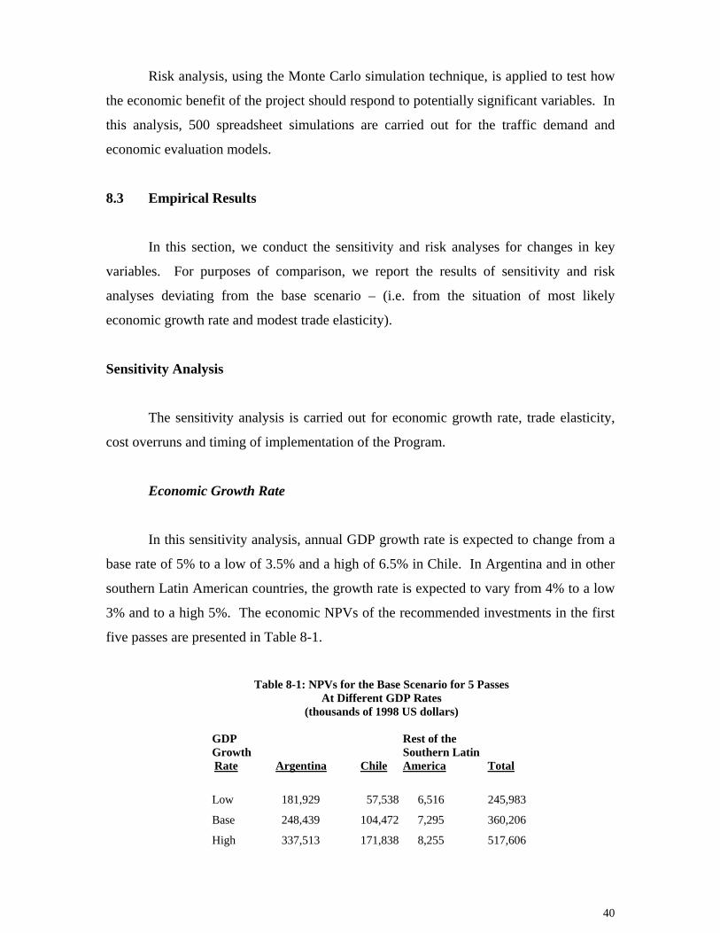
In this sensitivity analysis, annual GDP growth rate is expected to change from a
base rate of 5% to a low of 3.5% and a high of 6.5% in Chile. In Argentina and in other
southern Latin American countries, the growth rate is expected to vary from 4% to a low
3% and to a high 5%. The economic NPVs of the recommended investments in the first
five passes are presented in Table 8-1.
Table 8-1: NPVs for the Base Scenario for 5 Passes
At Different GDP Rates (thousands of 1998 US dollars)
GDP Rest of the Growth Southern Latin
Rate Argentina Chile America Total
Low 181,929 57,538 6,516 245,983
Base 248,439 104,472 7,295 360,206
High 337,513 171,838 8,255 517,606
40

The net economic benefits should increase in proportion to the GDP growth rates.
For example, the optimistic growth rate scenario should raise the levels of the net
economic benefits for both Argentina and Chile. In terms of percentage distribution of the
economic benefits between the countries, Chilean residents should gain more than
Argentinean residents, because annual GDP growth rates are expected to increase faster
in Chile (30% increase from 5%) than in Argentina (20% increase from 4%). On the
contrary, the pessimistic growth rate scenario is expected to raise the percentage
distribution of total net benefits for Argentina, because her GDP growth rates should not
decline as much as Chile’s.
Trade Elasticity
The import and export elasticities used in the demand model are assumed to be
1.5 for all commodities in Chile. In Argentina, the trade elasticity should range from 1 to
2, depending on the commodity. For the purpose of this analysis, the trade elasticity is
expected to vary by 20%. In other words, the low trade elasticities are assumed to be
80% of those used in the base scenario, while the high trade elasticities area assumed to
be 120% of the base ones. The economic NPVs of these simulations are presented in
Table 8-2.
Table 8-2: NPVs for the Base Scenario for 5 Passes
At Different Trade Elasticities (thousands of 1998 US dollars)
Rest of the Trade Southern Latin Elasticity Argentina Chile America Total
Low 197,170 70,936 6,772 274,878
Base 248,439 104,472 7,295 360,206
High 313,726 147,452 7,928 469,106
41

Trade elasticity also has a significant impact on net economic benefits. The
greater the trade elasticity, the more numerous the benefits that should be received by
Argentina, Chile and other southern Latin American countries. This is not surprising
because the greater level of trade should lead to a greater absolute response to changes in
prices for tradable goods.
Cost Overrun
The estimated costs for the program are based on the analysis of engineering
technical data at varying levels of detail for each pass. These estimates have been used as
the basis for the economic appraisal of the investment program. However, actual costs
could be higher or lower considering, the level of detail of the basic engineering studies
that have been conducted and the known physical conditions of the passes, including
topography and geo-technical conditions.
Considering the various factors affecting the risk of cost overruns, a range of
possible variation has been determined for each of the highway passes recommended for
improvement in the Program. The outer limits of the range are expressed in terms of
percentage variation from the expected value of the construction cost as shown in Table
8-3A.
Table 8-3A
Range of Variation of Construction Cost Estimates (percentage variation from expected Value)
Highway Pass Minimum Maximum
Jama -10.00 +20.00
Agua Negra -15.00 +30.00
Cristo Redentor -5.00 +10.00
Pehuenche -15.00 +30.00
Pino Hachado -10.00 +20.00
Huemules -10.00 +20.00
Integracion Austral -10.00 +20.00
San Sebastian -10.00 +20.00
42

This section examines the sensitivity of minimum and maximum capital costs on
economic viability. The results of these simulations are shown in Table 8-3B.
Table 8-3B: NPVs for the Base Scenario for 5 Passes
At Different Levels of Cost Overruns (thousands of 1998 US dollars)
Rest of the Capital South Latin Costs Argentina Chile America Total
Minimum Costs 264,367 117,189 7,295 388,851
Base 248,439 104,472 7,295 360,206
Maximum Costs 216,583 79,038 7,295 302,916
The economic NPV is expected to be affected by construction cost overruns.
However, the recommended program of investments in the five passes should remain
economically viable, even if cost overruns are high as 30% for all passes, because all the
benefits generated by the increased vehicle traffic should still remain intact.
Timing of the Project
In the analysis so far, the project has been assumed to begin construction in 1999.
In this section, we assume that the program will be delayed by one to two years. The
economic NPVs of these simulations are presented in Table 8-4.
Table 8-4: NPVs for the Base Scenario
At Different Beginning Years of Construction (thousands of 1998 US dollars)
Beginning Rest of the Construction South Latin Year Argentina Chile America Total
1999 248,439 104,472 7,295 360,206
2000 245,245 107,269 6,849 359,363
2001 240,733 108,798 6,424 355,955
43

The results indicate that there should be a reduction in the net economic NPV for
Argentina and other countries in southern Latin America, with the exception of Chile, if
the improvement of the five recommended passes is postponed for one year, because the
benefits generated by traffic will be lost forever, if the opening of the passes is delayed.
Risk Analysis
All the above analyses are based on deterministic values of input variables in the
model. This may not be a realistic assumption. The values of input variables should
vary, depending upon conditions in their respective markets. From the sensitivity
analysis, we found that the most important factors affecting the project’s economic
viability are GDP growth rates and trade elasticities. Cost overruns also affect the
present value of economic benefits, but to a lesser extent. Nevertheless, cost overruns are
always a concern to decision-makers. Therefore, we include these three variables in the
Monte Carlo risk analysis.
After risk variables are modeled, a set of Monte Carlo simulations is carried out.5
The analysis is conducted for the economic appraisal. The probabilities for GDP growth
rates are assumed to be 30, 40 and 30% for rates of 3.5%, 5% and 6.5%, respectively, for
Chile and for rates of 3%, 4% and 5% respectively, for Argentina and other southern
Latin American countries. The probabilities are assumed to be 30, 40 and 30% for the
low, medium and high elasticities. In the case of cost overruns, the probabilities are
calculated from the minimum and maximum ranges of construction cost estimates for
each pass (see Table 8-3A).
The outcome of the analysis is presented in Figure 8-1. The analysis shows that
there is no expectation of a negative economic net present value for the region. The
implementation of the recommended program of investments should significantly
improve the economic welfare of the residents in Argentina, Chile and the rest of
southern Latin America.
5 The risk analysis is done using the risk package called “Crystal Ball”.
44

Figure 8-1: ECONOMIC NPV FOR THE FIVE PASSES
(thousands of 1998 US$)
Summary:
Entire Range is from 171,574 to 738,608
500 Trials
Statistics:
Mean 388,696
Median 364,607
Standard Deviation 143,600
Range Minimum 171,574
Range Maximum 738,608
Cumulative Chart
.000
.250
.500
.750
1.000
0
125
250
375
500
150,000 300,000 450,000 600,000 750,000
500 Trials 0 Outliers
Forecast: Net Economic Benefits NPV
45

9 CONCLUSIONS
In this study, we have developed an analytical framework to evaluate various
passes in the Andean highway program and have suggested a recommended program of
investments. The recommendations reflect the economic net benefits expected for the
region of southern Latin America. The benefits forecast for the economies of Argentina,
Chile and the rest of the region as well as for different sectors of the economy are
presented in the report.
To evaluate the economic viability of the investment projects, we integrate the
engineering cost estimates, the conversion factors for translation from financial costs to
economic costs, and the forecasts of passenger and freight traffic into a stream of
economic costs and benefits over the life of the project. The traffic forecasting is based
on the model developed separately in this study. The traffic forecast, together with
vehicle transportation costs and time savings, are then translated into the measurement of
economic net benefits.
The main conclusions are summarized as follows:
• Ten of the 11 passes under consideration in the Andean highway program (with the
exception of San Francisco), when paved, should each make a positive contribution
to the economy of southern Latin America as a whole. The net present value for
economic benefits ranges from US$201 million (in 1998 prices) for the Pehuenche
pass to US$2.2 million for the Huemules pass. For the San Francisco pass, the net
present value is negative. In other words, from an economic point of view, this
pass should not be improved under the current program.
• Some passes compete with each other, since they serve the same market. Building
them simultaneously would result in a considerable reduction in net economic
benefits. These pairs of passes include: Jama and Sico, Pircas Negra and San
Francisco, Pehuenche and Cristo Redentor, and Pehuenche and Pino Hachado.
This is especially true in the case of Jama and Sico and Pircas Negra and San
Francisco.
46

• The empirical simulations suggest that the recommended program of investments
should include Jama, Pehuenche, Cristo Redentor, Agua Negra and Integracion.
They are expected to generate approximately US$360 million in present value of
net economic benefits, expressed in 1998 prices. These five passes would provide
the greatest economic net benefits, and they are considerably well advanced in
terms of planning. The subsequent investments in three additional passes, Pino
Hachado, San Sebastian and Huemules, should also generate a positive net present
value to the economy of the region. The remaining three passes are not expected to
contribute any economic benefits to the region.
• In terms of distributive benefits, approximately 69% of the economic benefits
should accrue to the economy of Argentina, 29% to the economy of Chile and 2%
to the rest of the southern Latin American countries. Producers in Argentina and
Chile should benefit the most from construction of the highway passes. Passengers
in both countries should also gain access to an improved highway system. The
governments of Argentina and Chile are expected to lose the most from a
government budget perspective, due to expenditures, which will be required for
improving this infrastructure.
• It is interesting to note that with substantial investments in the public sector
infrastructure, the governments of Argentina and Chile should receive taxes and
import duties associated with capital expenditures and maintenance costs in the
present value of US$33.7 million and US$23.7 million, respectively.
• The results of the economic analysis are sensitive to a number of variables such as
economic growth rates and trade elasticities. They are also affected by cost
overruns during the construction period. Nevertheless, with a maximum of 30%
cost overruns, the recommended program of investments should still generate a
considerable amount of economic benefit in the southern Latin America region as a
whole. It should also be noted that there is expected to be a reduction in economic
benefits if the construction of the recommended program of investments is
postponed, because of the associated loss in the value of transportation services
foregone through delay.
47

Appendix A. THE MACROECONOMIC FORECAST A.1 Introduction
A host of internal and external factors determines the economic growth prospects
of an economy. Each factor, by itself, is difficult to predict over a long period of time.
Furthermore, the prospects for future growth often change in the short-term, making the
business of long-term projections a challenging one.
This study uses a standard growth model, derived from a Cobb-Douglas
production function, to construct long-term projections for economic growth in Chile and
Argentina. The role of international trade in the growth of each economy is analyzed in
the context of this model approach, with particular attention to the impact of regional
trade liberalization.
A.2 Growth Model
Modern growth analysis is based on equation (A-1), in which the contributions of
labor and capital to economic output are disaggregated, along with a residual.6 In other
words, an increase in GDP (∆Y) can be measured by the sum of the increase in factor
incomes – real wages and capital income – and a residual item which can be categorized
as the reduction in real costs, or the increase in factor productivity. Thus, the change in
GDP for any year can be expressed in the following manner:
∆Y = ω • ∆L + (ρ + δ) • ∆K + R (A-1)
where ω is the average rate of return to labor, ρ is the average rate of return to capital, δ
is the average rate of depreciation of capital stock, ∆L is the change in the labor force,
∆K is the change in the country’s capital stock, and R is the reduction in real costs. Thus,
growth in GDP can be attributed to an increase in the labor force, the capital stock, the
average return to capital and labor, and the overall “total factor productivity”.
6 See Harberger, Arnold C., “Reflections on Economic Growth in Asia and the Pacific,” Journal of Asian Economics, (1996), Vol. 7, No. 3, pp. 365-392.
48

Equation (A-1) can be rearranged to express the change in GDP in terms of a
growth rate or percentage change. The annual GDP growth rate (∆Y/Y) is therefore
derived as follows:
∆Y Lω ∆L ∆K R ⎯ = ⎯ • ⎯ + (ρ + δ) • ⎯ + ⎯ (A-2) Y Y L Y Y
where Lω is the share of labor to total factor income, ∆L/L is the growth rate in the labor
force, ∆K/Y is the ratio of the increase in capital stock to GDP, and R/Y signifies the
reduction in real costs, or the increase in total factor productivity expressed as an annual
percentage change.
Equation (A-2) can be used to project economic growth by making assumptions
about the future values of each variable, a process which should be informed by historical
precedent, but ultimately informed by judgment regarding future expectations. Any
projections of future growth informed by historical trends must be conducted carefully.
Future predictions should be guided by the historical time period chosen and should be
particularly sensitive to the effect of business cycles and external shocks when dealing
with Latin American economies. Evidence indicates that there can be large short-term
movements in total factor productivity associated with business cycles.
Future economic, fiscal and monetary policies will clearly have a major impact on
long-term sustainable economic growth, and our judgment forms the basis for predicting
future government policies in Chile and Argentina. In addition, external factors such as
the economic and investment conditions within major trading and investment countries
should also influence growth in the long run. Our projections account for these
considerations.
49
A.3 Empirical Analysis – Chile
A.3.1 Macroeconomic Forecast
By 1997, the Chilean economy had registered 14 consecutive years of growth,
with real growth rates during the 1984-1996 period averaging 6.6% per year, and income
per head doubling. Appendix A-1 provides an overview of Chilean macro-economic
indicators since 1991. Growth during this recent period has been driven by heavy export
growth (averaging of 9.8% annually) and by increasing investment. Gross investment in
fixed capital stock has expanded at 12.3% per annum between 1990 and 1996. Total
investment has averaged more than a quarter of GDP for the past six years.
The growth equation provides a mathematical means of constructing predictions
for future economic growth in Chile. The value for each variable within the equation
must itself be a predictor of future conditions in the Chilean economy. To predict future
growth, information available on the sources of previous economic growth in Chile is
reviewed below. Given that much of the economic reform and stabilization which has
driven growth in Chile and which sets the stage for future growth has occurred over the
past decade, our projections are guided in large part by recent economic performance
since 1990.
Labor Input Contribution
Recent data on Chile’s labor force is not readily available. Statistics on average
population growth over the past five years for which there is data (1991-95) indicate an
annual average increase of 1.63%.7 We can assume a similar growth in the labor force
over time of 1.6%, which is about the same assumption used in Marfan and Bosworth’s
basic growth scenario (1994). Following Gregorio, we use 60% as a value for the share
of labor to total factor income in Chile and anticipate that this proportion should continue
relatively unchanged.8
7 International Monetary Fund, International Financial Statistics, (December 1997).
50

Capital Input Contribution
Marfan and Bosworth (1994) use an implicit annual depreciation rate of 5 percent
in their projections of future economic growth in Chile, which seems to be reasonable
and is therefore employed in our calculations. The real rate of return to capital is
expected to be 6% in the medium to long-term, as the economy improves its
competitiveness and efficiency in response to trade liberalization and deregulation. In
fact, the 6% figure proves to be a quite robust estimate for a number of countries.
Based on Marfan and Bosworth’s (1994) estimates, the average capital-output
ratio in Chile was calculated to be 2.2 during the past three decades preceding 1992. The
annual increase in capital stock varied, depending upon annual depreciation of the stock
and annual gross investment. We anticipate that investment as a percentage of GDP
should remain at more than 25%, and thus anticipate continued growth in capital stock at
approximately 4%. Due to the expanded gross investment in recent years, one would
expect an increasing capital-output ratio in Chile in future years, and we therefore assume
that it should increase to 2.5, a level comparable to that of the U.S., Canada, and other
industrialized nations.
Total Factor Productivity Contribution
Robles (1997) calculated that the total factor productivity (TFP) increased by
approximately 3.0% annually since 1985, and contributed almost half of GDP gains
during that period. A key issue in interpreting TFP gains during the period is the extent
to which recent gains are indicative of fundamental economic trends or more short-term
cycles. While Marfan and Bosworth (1994) argue that recent TFP gains are reflective of
the economy’s position in the business cycle, it seems more reasonable to impute such
gains to underlying trends in light of continued growth since 1993 and continuing
economic reforms. Long-term growth in TFP at a level of 3.0% seems feasible in light of
ongoing economic reform and continued stable macro-economic conditions. Inflation
has been steadily declining over time, dropping from 8.9% in 1994 to 6.6% in 1996.
8 Gregorio employed 60% for the labor to total factor income figure for his projections of future growth in Chile. See Gregorio response in Marfan and Bosworth (1997).
51

Several factors influence TFP, and in Chile the critical issues will be
technological progress and increasing the labor force’s skill level. Success in both areas
will be necessary in order to sustain an annual increase in TFP of 3.0% in the long run, as
will continued effectiveness in maintaining a stable macro-economic environment. The
Chilean government has followed conservative fiscal and monetary policies, which seem
relatively certain to continue, given broad political support for the Concertacion.
We assume, therefore, that reforms currently underway should be successful in
raising the level of human capital in Chile over time to meet the need for a workforce
capable of competing in global markets. As Chile faces growing competition through
liberalized trade, it will be increasingly important for the country to develop trained
managers and workers to cope with technological progress and to drive innovation. Chile
is presently engaged in developing needed educational infrastructure, lengthening the
school day and year, and investing in teacher training. Improving education and reducing
poverty were Mr. Frei’s top stated policies through 2000.
There are also trends, which suggest that technological advances should improve
productivity in Chile in the long run. The proportion of capital goods in Chilean imports
has been on the rise, currently standing at approximately 27% of imports, a percentage
which is anticipated to rise slightly over time. These increased capital goods bode well
for productivity increases, as it is widely considered that capital intensive goods provide a
dynamic effect for an economy through technology diffusion not possible through less
value-added products.
Employing the above assumptions, parameter values for the base case scenario are
summarized in Table A-1.
Table A-1: Parameter Values and Base-line Growth Projections
Parameter Values for Chilean Growth Lω / Y= 60% ∆L/L = 1.6% ∆K/Y = (∆K/K)(K/Y) = 10.0% R/Y = 3% ρ = 6.0% δ = 5.0%
52

Base-line results Labor input Capital input Total factor productivity Total expected GDP growth 1.0% + 1.1% + 3.0% = 5.1%
Thus, the annual GDP growth rate in the next 20 years is projected to be 5.1% for
Chile. This growth rate assumes that infrastructure will develop as needed in order to
provide transportation for increasing trade and development, for which the present system
is rapidly becoming inadequate. The contribution of capital input to the annual GDP
growth rate is estimated to be 1.1% in the base case, which is substantially lower than the
figures of 2.8% and 3.3% calculated by Robles (1997) for the periods 1985 to 1990, and
1990 to 1994, respectively. If the contribution of capital to growth continues in future
years, Chilean annual growth rates would be even higher. Moreover, if Chile joins
NAFTA, additional GDP gains of approximately 1.47% per annum could accrue, as
Harrison, Rutherford and Tarr (1997) calculate using a CGE model. It is therefore
assumed that the optimistic growth scenario for Chile should be 6.5% over the next 20
years.
On the other hand, as the Chilean economy continues to open up to Latin and
North American countries, as well as the Pacific Rim, her economy should also be
influenced by external factors. In addition, her major exported commodities should be
subject to volatility in world markets, which could have a negative impact on the
economy, unless diversification of exports occurs at a sufficient rate. Chile’s strong
reliance on exports to drive growth and stagnation in trading partner economies such as
East Asia in recent months could have a powerful downward effect on growth.
Therefore, we consider a 3.5% growth rate to be the pessimistic long-run scenario.
A.3.2 Other Studies of Growth
Table A-2 presents the historical contribution of labor, capital, and total factor
productivity to output in Chile, as calculated by Robles (1997), during five year time
intervals from 1960-1994. Robles also find a strong correlation between total factor
productivity increases and overall GDP increases in Chile, which accounts for 58% of the
growth over time.
53

Table A-2: Contributions of Inputs to Growth Rates for Chile, 1960-1994
1960-1965
1965-1970
1970-1975
1975-1980
1980-1985
1985-1990
1990-1994
Output (GDP) 3.8% 4.8% -2.0% 7.5% -0.1% 6.5% 7.2% Labor Input 1.1% 1.9% 0.7% 0.8% 0.6% 1.0% 0.9% Capital Input 1.8% 2.1% 1.2% 1.6% 1.1% 2.8% 3.3% Total Factor Productivity
0.9% 0.8% -3.9% 5.2% -1.8% 2.8% 3.0%
source: Edgar Robles, An Exploration into the Sources and Causes of Economic Growth in the United States and Fourteen Latin American Countries, Ph.D. Dissertation, University of California, Los Angeles, (1997).
We have conducted a review of existing economic and trade forecasts for Chile
prepared by government, private sector and international organizations. Medium term
forecasts for real GDP growth range from 5.9% (WEFA) to 7.2% (EIU). Projections of
real export growth range from 7.3% (EIU) to 11.5% (PECC), while real import growth is
predicted to grow between 7.1% (WEFA) and 12.5% (EIU). Details expressed in
percentage are shown in Table A-3.
Table A-3: Economic and Trade Forecasts by Various Organizations, 1997-2000
(percentage) 1997 1998-2000 Forecasts Official IMF PECC DRI WEFA EIU PECC DRI WEFA
Real GDP 6.0 5.5 5.6 5.4 5.1 7.2 6.3 6.7 5.9 Real Exports 11.0 n/a 7.6 7.6 10.4 7.3 11.5 10.3 7.4 Real Imports 6.0 n/a 7.1 8.8 10.9 12.5 8.8 10.4 7.1 CPI 5.5 6.0 5.5 6.2 6.2 4.6 4.5 4.3 5.0
Notes: The IMF forecast is from the World Economic Outlook (IMF, September 1997); figures for the period 1998-2000 refer to 1998 only. The PECC forecast is from the Pacific Economic Outlook 1997-1998 (PECC, 1997); 1998-2000 figures refer to 1998 only. The DRI forecast is from World Market Executive Overview (3rd Quarter, 1997). The WEFA forecast is from Asia Economic Outlook (August, 1997). The EIU forecast is from Country Profile, 4th Quarter 1997, and averages are forecast for 1998 and 1999. Note: DRI and WEFA figures for real export and real import growth include services, while EIU import and export figures are for merchandise trade only.
The Central Bank of Chile anticipates that medium-term growth rates should
range between 6 and 7 percent, which they estimate to be Chile’s potential growth rate.9
The full macro-economic forecast generated by CIEPLAN and submitted to the UN as
part of the LINK program is included in Table A-4. CIEPLAN projects that real GDP
growth in Chile should continue at levels of approximately 6.3% through 2000, and
forecasts that real exports should grow, albeit at declining levels, over the next three
years: 9.8% (1998), 7.9% (1999), and 6.9% (2000). Imports are projected to grow at
6.0%, 5.9%, and 8.3% during the same years.
54

Table A-4: Project Link Macro-Economic Projections for Chile by CIEPLAN
1997 1998 1999 2000 Aggregate Demand (millions of 1986 pesos)
GDP 7,224 7,678 8,156 8,675 Private consumption 4,986 5,202 5,479 5,803 Government consumption 569 581 594 608 Change in stocks 235 250 255 365 Fixed Investment 2,069 2,211 2,364 2,528 Exports (Goods and Services) 2,865 3,145 3,393 3,627 Imports (Goods and Services) 3,501 3,711 3,929 4,256 Trade and Current Account (billions of Current US$)
Exports 16,436 18,429 20,308 21,958 - Copper 6,743 7,960 8,791 9,314 - Traditional Non-Copper 4,889 5,091 5,476 5,841 - Other 4,803 5,379 6,041 6,803 Imports 17,458 18,699 20,490 22,714 - Consumption 3,172 3,122 3,304 3,629 - Oil 1,296 1,295 1,000 922 - Intermediate Non-Oil 9,564 10,474 11,671 12,989 - Capital 4,801 5,094 5,742 6,376 Trade Balance -1,023 -270 -182 -756 Financial Services -2,509 -3,120 -3,568 -3,594 Non-Financial Services -241 -340 -464 -536 Transfers 512 551 589 626 Current Account Balance -3,261 -3,179 -3,643 -4,260 Other variables
CPI (% change) 5.5 5.0 4.0 4.0 Exchange rate (Pesos/US$) 419 421 423 425
Source: CIEPLAN, Santiago, Chile, prepared by Pablo Cabezas, submitted to the UN, September 1997.
The World Bank, in its country report on Chile, projected the medium-term
growth rate between 6.5 and 7.0%, provided that capital formation continues at a rate of
between 25 and 30 percent of GDP. The Bank also notes that education reform and a
revamping of the process for granting concessions for public works, as well as financial
deregulation, are key challenges, which must be addressed for sustainable growth.
Manuel Agosin (1997) of the University of Chile recently constructed long-run
projections for the Chilean economy through 2020, in which he forecast a real GDP
growth rate of 7.7%. The assumptions underlying Agosin’s endogenous growth model
are relatively strict, and include growth in the investment rate from 25 percent to 37
percent by the year 2020, investment in education at a level of 6.5% of GDP, and a rise in
public investment to 7 percent of GDP. 9 Chilean submission to APEC, in APEC, 1997 World Economic Outlook, Chile.
55

Professor Jorge Desormeaux at the Catholic University of Chile has suggested
that there are three basic scenarios for future growth contingent upon external economic
conditions and the domestic political situation.10
• Best case scenario, 7-8%: The best case scenario requires macro-economic
stability and active government involvement in the privatization of public
enterprises, as well as further deregulation of financial markets, reduction in
personal income taxes, and tighter fiscal policy. Desormeaux adds that greater
flexibility in labor legislation and an improvement in the educational system will
be necessary to realize this “tiger-like” pace.
• Intermediate case scenario, 6-6.5%: Under Desormeaux’s intermediate case
scenario, the Concertacion does not achieve the necessary political consensus to
modernize the economy completely and suffers from reduced growth as a result.
• Worst case scenario, 3-4%: Desormeaux’s worst-case scenario is indeed unlikely
and would entail a recession in important trading partner markets, as well as a
protectionist response from Chile, which would then harm private sector
competitiveness.
Table A-4 presents the forecasts submitted to the UN by the Chilean government
for a variety of macro-economic variables, including GDP and trade flows.
A.3.3 Future Trade and Implications for Future Growth
Background
Trade has been a critical driver of economic growth in Chile, with merchandise
exports as a percentage of GDP presently at 45.6%, far higher than in Latin America as a
whole, as Table A-5 indicates. As a result, the Chilean economy is highly dependent on a
continuing level of demand for exports.
10 Desormeaux, Jorge, “Economic Scenarios for Chile,” 1995 working paper.
56

Table A-5: Relative Significance of Trade to Latin American Countries and US in 1995
Argentina Columbia Chile Brazil U.S.A.
Total Merchandise Trade
as a % of GDP
14.1% 30.0% 45.6% 13.7% 18.3%
Source: IMF, International Financial Statistics.
In comparison to other Latin American countries, Chile’s exports are heavily
concentrated in processed and unprocessed natural resources, which constituted 87.2% of
all exports in 1994.11 Nearly 40% of Chilean exports are copper and copper derivatives,
while fresh fruit represents nearly 8%, and wood pulp and fishmeal each account for 4%.
See Appendix A-4 for more detail on the commodity structure of Chilean trade in 1996.
Given the volatility of commodity prices in world markets, Chile’s export structure is a
cause for concern, unless greater diversification is achieved over time.
There has been a growing trend, however, away from natural resources in exports,
which declined as a proportion of the total from 66.1% in 1986 to 51.7% in 1994.
Processed natural resources increased their share of exports from 29.4% to 35.5%, while
other industrial products tripled their share of exports from only 4.5% in 1986 to 12.8%
in 1994. See appendix A-5 for data on the changing structure of Chilean exports since
1986.
Chile’s primary trading export markets include the U.S. (17% of the total), Japan
(16%), South Korea (6%), the UK (6%), and Brazil (6%). In terms of sources of imports,
the U.S. sends the most goods and services to Chile, followed by Argentina, Brazil, Japan
and Germany. In terms of regional trade, most of Chile’s exports go to Asia, followed by
Europe, Latin America, and North America, as Table A-6 indicates.
There has been a considerable change in Chile’s trading partners over the past
decade. Exports to Mercosur countries have been on the increase, climbing from 8.2% in
1985 to 10.8% in 1995. While a majority of exports once went to the EU, that proportion
declined to 27% by 1995. NAFTA countries have similarly decreased in relative
11 Agosin, Manuel, “La Insercion Internacional de la Economia Chilena,” CEPRI, (May 1997).
57

importance as export markets for Chile, declining from 26.1% in 1985 to 15.8% in
1995.12
Table A-6: Trade by Region in Chile, 1995
(as a percentage of total)
Region Exports Imports
North America* 15.0 26.8
Latin America 18.8 26.8
Europe 29.4 22.3
Asia 34.0 16.9
Rest of world 1.8 3.5
*excluding Mexico
It is likely that the current structure of trade will change significantly over the
long-term, since the sectoral composition of the economy should also change as the
economy develops. The natural-resource-weighted nature of Chilean exports should
likely decline over time and the relative importance of industrial goods and services
should increase, in keeping with the experience of other developing economies. Copper
and its derivative products are expected to remain an important part of Chilean exports.
COCHILCO, the Chilean Copper Commission, has undertaken a biannual
assessment of world copper markets, releasing its most recent study in 1996. In its study,
COCHILCO projected that copper exports would continue to increase in line with
previous growth. Nevertheless, given that capacity in Chile is increasing rapidly and that
demand cannot be expected to keep up in the long run, exports are forecast to decline in
significance, although they will continue to increase in real terms. The Commission
forecasts that copper production should increase to 3.1 million tons by the year 2000, a
47% increase over 1995 levels.13
Agosin projects that exports of manufactured goods should increase from a 23%
share of the total in 1995 to 43% by the year 2020, and that exports of services should
rise from 16% of the total in 1995 to 29% in 2020.14
12 Ibid. 13 Estrategia, October 17, 1996.
58
Regional versus Multilateral/Unilateral Tariff Reduction
There is a debate in Chile over which strategy is expected to lead to greater
market access and economic benefits. Regional trade agreements can lead to the
application of greater tariffs on goods and services from outside the trade area. In the case
of Chile, which already imposes a relatively low and uniform tariff, it is particularly
critical that trade agreements should lead to improved market access.
Butlemann and Meller (1995) argue that Chile should negotiate bilateral free trade
agreements (FTA’s) with as many trade partners as possible, while Donoso and Hachette
(1996) argue that some bilateral agreements, such as Mercosur, provide limited benefit in
improved access and are therefore not worth the delay in liberalizing other trade. Some
evidence from the recent structure of intra-Mercosur trade suggests that barriers applied
to regional trading have led to trade in goods in which Mercosur nations have little
competitive advantage in world markets (Yeats 1997).
Mercosur
Chile entered Mercosur as an associate member in 1996 in an agreement, which
became operational in October. Under the agreement, the average weighted import tariff
faced by Chilean exports in Mercosur countries dropped from 8.2% to 3.2%, while
import tariffs from Mercosur fell from 8% to 5.7%.
Harrison, Rutherford and Tarr (1997) use a Ramsey dynamic model to predict the
impact of Mercosur on Chile and conclude that its overall impact would be mildly
negative on the order of -0.56% in real GDP for an FTA and -0.44% for a customs union,
depending upon the assumptions regarding trade elasticities. Their conclusion is
generally supported by other models generated by Donoso and Hachette (1996) and
Muchnik, Errazuriz and Dominguez (1996). However, Harrison’s model does not allow
for the impact of trade with industrialized partners, which could lead to added
productivity through technology transfer. Another model focused on the added impact of
14 Agosin, Manuel, “Un Modelo De Proyeccion de Largo Plazo Para La Economia Chilena,” 1997.
59

technology transfer yielded positive results for Mercosur and an even greater positive
impact for NAFTA.
Harrison et al. (1997) employ their computable general equilibrium (CGE) model
to predict the impact of Mercosur on trade and output by industrial sector as well. The
model projects the incremental impact of tariff reductions under the agreement, using
1992 figures. The results indicate that the percentage impact of Mercosur tariff
reductions should be most significant in the transportation industries, although the
industry contributed less than 1% of GDP and 2% of the value of exports.
NAFTA
Chilean exports presently face relatively low tariff barriers in the U.S.
(2.5%), Canada (3.6%), and Mexico (2.9%).15 Given that there is an 11% tariff on
NAFTA products, an FTA with NAFTA would likely have a large impact on imports.
Harrison, Rutherford, and Tarr (1997) use a Ramsey dynamic model to predict the impact
of NAFTA on Chile and conclude that its effect on real GDP would be an increase of
1.47%. The positive impact would come largely as a result of improved access to
NAFTA country markets, in particular for non-grain crops into the U.S., which presently
have 20% tariffs16 on average.
Valdez (1996) employs a partial equilibrium model to calculate the commercial
effects of free trade and finds that exports should increase by 4.4% and imports by
27.5%, of which 16.3% would be new commerce and 11.2% would be shifted from
elsewhere.
European Union
Most Chilean goods currently exported to the EU are faced with a negligible tariff
barrier. Copper, metals, cellulose, furniture, and fishmeal constituted 74.9% of exports to
the EU in 1994, and all entered the market almost free of tariffs (Alvarez 1996).
15 Agosin, Manuel, “La Insercion Internacional de la Economia Chilena,” p. 25. 16 Harrison et al. “Trade Policy Options for Chile.”
60

However, there are other Chilean goods that are not presently exported to the EU which
are blocked by high tariffs, in particular17 agricultural goods.
There is a possibility in the long run that Chile will enter into a free trade
agreement with the European Union (EU). Alvarez (1996) calculates that the net
economic impact of free trade with the EU should be a 1.7% real increase in GDP. He
concludes that the impact of eliminating trade barriers between the EU would be to raise
exports by 3.9% in the short-run and 10.3% in the long run, while boosting imports by
26.6%. Import breakdown would be 16.3% new commerce and 10.3% diverted
commerce.
There are additional trade issues. As noted, the Chilean economy relies heavily
on exports to drive growth at a higher level than other Latin American countries. This
reliance makes Chile vulnerable to macroeconomic conditions which affect its trading
partners. The recent crisis in East and Southeast Asia illustrates Chile’s vulnerability. In
addition, an increased foreign capital flow into Chile in recent years has contributed to a
continuing appreciation of the peso, with implications for export trade.
A.4 Empirical Analysis – Argentina
A.4.1 Macroeconomic Forecast
Argentina registered successful GDP growth between 1991 and 1994 of 7.7%
until the Mexican crisis of 1995, when Argentina experienced a sharp recession, which
led to a 4.4% reduction in GDP. Since then, the economy has begun to recover, growing
by 4.25% in 1996 and by an estimated 7.5% in 1997. Prior to 1990, the economy had
been stagnant as a result of a combination of ineffective fiscal, trade and monetary
policies.
The basic growth equation (A-2) is used as a framework for projecting long-term
economic growth in Argentina. For the purpose of guiding projections, historical data for 17 Agricultural goods exported to the EU presently face ad valorem equivalent tariff rates of between 0 and 489%, with an average of 15%, while farm goods face an effective rate of between 0 and 177%, with an average of 14%. See Agosin, Manuel, “La
61

Argentina’s performance with these different variables is reviewed. Given that economic
and trade reform did not substantially begin in Argentina until 1989, more recent
economic data is used as a guideline.
Labor Input Contribution
Given persistent unemployment rates in Argentina, we have estimated a ratio of
labor income to total factor income of 50%, lower than the 60% assumed for future
growth in Chile.
Recent figures on the size of the labor force (1986-1993) indicate growth of 0.8%
annually.18 There are also projections for long-term general population growth from the
Argentinean government, which suggest that the population is expected to grow to 41
million by 2010 and 45 million by 2020, implying an annual rate of increase of
approximately 1.1%.19
We assume that the labor force should increase in the long run at a rate of 1.25%,
higher than previous historical growth, because of workers discouraged by the high
unemployment rates of 17% in October 1996. The unemployment rate is expected to
drop several points in the short term, and more over time, as labor laws are reformed and
privatization continues.
Capital input contribution
Given a slightly lower level of industrialization in Argentina than in Chile, we
have employed a 4% depreciation rate for capital stocks20 and utilized a 3% rate of
increase in the capital stock. With this assumption plus the ratio of 2 for the capital-
output ratio, one would expect the ratio of change in capital stock to GDP to be about
6.5%. The rate of return to capital is also considered, in line with the experience
recorded in other developing countries, to be 6 percent for the foreseeable future.
Insercion Internacional de la Economia Chilena,” p. 24. 18 INDEC, Encuesta Permanente de Hogares. 19 INDEC-CELADE, 1996, Serie Analisis Demografico 7. 20 The aggregate depreciation rate is a weighted average of 2.5% for structure and 8% for machinery and equipment.
62

Total Factor Productivity (TFP)
Argentina has registered strong growth in real GDP since 1990, with the
exception of 1990 and 1995 (0.06% and -4.4%, respectively). For the entire period, the
annual growth rate has averaged 4.38%, which would imply a reduction of real costs on
the order of 3.10% over the past seven years, given our assumptions regarding labor and
capital contributions to growth. Continued growth in TFP in Argentina is feasible, in
light of the previous performance, and reflecting trends of increasing trade liberalization,
privatization, and labor reform. Growing confidence in the government and the economy
also bode well for the future success of these efforts.
Increasing imports of capital goods also suggest a future increase in TFP through
the diffusion and transfer of technology. The level of imports of capital goods has
increased, both as a percentage of imports (from 19.8% in 1990 to 29.9% in 1995) and in
absolute terms (from $807 million to $6,016 million during the same period21). The
increasing proportion of capital goods bodes well for long run productivity in Argentina.
As noted in Chile’s case, capital goods are expected to have a positive impact on
productivity in the importing country as result of the diffusion or transfer of technology
in goods.
For these reasons, we suggest that a medium-to-long term value of approximately
2.72% increase in TFP is not unreasonable for Argentina. That value should yield a long-
term real GDP growth rate of 4 percent as a baseline, as indicated in Table A-7.
Table A-7: Parameter Values and Base-line Growth Projections for Argentina
Parameter Values for Argentine Growth
Lω / Y= 50% ∆L/L = 1.25%
∆K/Y = 6.5% R/Y = 2.72%
ρ = 6.0% δ = 4.0%
Base-line results
Labor input Capital input Total factor productivity Total expected GDP growth
0.6% + 0.7% + 2.72% = 4.0%
21 ECLAC; IMF, Direction of Trade Statistics, 1997.
63

Thus, the annual growth rate in Argentina is projected to be 4.0% in the base-case
scenario, which is in line with the previous growth recorded in the economy. This long-
term growth rate assumes that Argentina can manage several issues, which threaten to
restrict growth, especially the need for increased investment in infrastructure.
In the long run, the Argentinean infrastructure will clearly need to be upgraded to
deal with greater development and trade flows, as trade within Mercosur increases. The
three corridors between Argentina, Chile and Brazil,22 the Buenos Aires port, and cargo
trans-shipment facilities will need to be developed to manage increased trade and enable
continued economic growth. For example, an analysis by the Japanese International
Cooperation Agency (JICA) projected that Argentina would handle container volume of
0.97 million TEU’s by 2000, 1.24 million TEUs by 2005, and 1.6 million by 2010.23
JICA concluded that significant new capacity needs to be developed outside of Buenos
Aires in order to handle anticipated volumes.24
Since the base-line scenario for future growth is 4 percent, increased dynamic
impacts from trade liberalization and deregulation of the financial and labor markets may
lead to added benefits in productivity and drive slightly higher capital investment, which
could boost growth to 5 percent in an optimistic scenario.
On the other hand, there remain issues with the political and legal system in
Argentina, persisting unemployment, and the stability of reform which could, in a
pessimistic scenario, pull growth down to a 3 percent level.
A.4.2 Other Studies on Growth
We have reviewed existing forecasts for economic growth, trade, and other
macro-economic indicators by the Argentinean government, private firms, academics,
and international organizations. Forecasts for medium to long-run growth range from
3.8% (Economist Intelligence Unit) to about 5.6% projected by the Ministry of the
22 Iquique to Sao Paulo via Jujuy, Valparaiso to Sao Paulo via Mendoza and Buenos Aires, and Concepcion to Bahai Blanca via Neuquen. 23 OKITA, OKITA Final Report, Issue 4. 24 Ibid.
64

Economy of Argentina, with World Bank projections of 4 % to 5 %, in the middle range.
Details are shown in Table A-8.
Table A-8: Forecasts by Various Organizations for Growth in Argentina
1997 1998-2000
Forecasts Actual Official WEFA EIU
Real GDP 8.0% 5.8% (1998)
5.6% (1999)
5.4% (2000)
5.0% (1998) 3.8% (1998)
4.0% (1999)
Real Exports 13.3% 12.8% (1998) 4.8% (1998)
3.2% (1999)
Real Imports 24.8% 12.3% (1998)
7.5% (1999)
CPI .5% 1.1% (1998)
2.0% (1999)
2.0% (2000)
1.9% (1998)
2.9% (1999)
Notes: Official forecast is from Economic Report No. 22: The Argentine Economy in the Second
Quarter of 1997; Economist Intelligence Unit forecasts are from Country Report: Argentina, 4th
Quarter, 1997; Forecasts are averages for 1998 and 1999 only; Trade statistics are for
merchandise only; WEFA forecast is from “Latin American Highlights,” Eddystone, PA,
(October 1997).
In its publication, Trends in Developing Countries 1996, the World Bank
forecasts that real GDP growth in Argentina will range between 4 % and 5%, assuming a
full recovery, continuing economic adjustment through restructuring of the financial and
labor markets, reform of the health insurance system, and a continued flow of private
capital into the economy.25 A full listing of the Argentinean government’s projections for
growth, trade, and other macro-economic indicators is contained in Table A-9.
25World Bank Group, Trends in Developing Countries 1996, Argentina Country Overview.
65

Table A-9: Argentinean Ministry of the Economy Forecasts, 1998 to 2000
Indicator 1997 1998 1999 2000
GDP (millions of 1986 pesos)
13,852 14,658 15,479 16,315
Real GDP Change 7.5% 5.8% 5.6% 5.4%
Gross Domestic Investment as
% of GDP
20.2% 21.9% 22.8% 23.7%
Balance of Payments
(millions of current pesos)
- Current Account Projections
Merchandise -1,241 -2,051 -1,834 -1,349
- Exports 26,514 29,531 33,390 37,539
- Imports -27,755 -31,581 -35,224 -38,888
Real Services -2,867 -3,320 -3,681 -4,019
- Income 3,601 3,929 4,315 4,723
- Expenses -6,468 -7,250 -7,996 -8,742
Yield on Investment -5,165 -5,424 -6,192 -7,170
- Profits and dividends -2,549 -2,999 -3,449 -3,966
- Net Interest -2,616 -2,425 -2,743 -3,204
Transfers 336 333 329 326
- Capital Account 10,908 12,782 13,729 14,707
Foreign Direct Investment 4,337 4,987 5,735 6,596
Other Capital Movements 1,970 2,320 2,350 2,495
Source: Ministry of the Economy, Economic Report No. 22, Second Quarter 1997.
A.4.3 Trade and Implications for Future Growth
Background
Argentina’s trading patterns have changed rapidly since the country began to
reduce tariff and non-tariff barriers to trade. The economy’s participation in the world
market remains relatively small in comparison with its Latin American counterparts.
While the importance of trade to the Argentine economy is below overall Latin American
levels, it has nevertheless been increasing over time. Total merchandise trade as a
percentage of GDP now stands at 14.1%.
66
Argentina’s trading partners have changed significantly since the 1980’s, when
most exports went to the EU and the U.S. By 1993, this pattern had shifted in favor of
Mercosur, which comprised 28% of exports, and the EU continued to take 28% of the
total, as it did in the late 1980’s. Brazil is now the biggest buyer of Argentinean products
(21%), followed by the US (10%). By 1996, trade with Mercosur countries, including
Chile, represented 40.7% of all exports and accounted for 26.8% of all Argentina’s
imports. The overall quantity of trade by region and country is contained in Appendix G
for the period 1994-96.
The commodity structure of Argentinean imports has also changed over the past
decade toward manufactured goods and away from primary goods. Manufactured goods
increased as a share of total exports from 18% in 1985 to 28% in 1993, while primary
products dropped from 44% to 25% during the same period.26 Appendix H provides a
detailed listing of the volume of Argentina’s recent trade flows by commodity type for
the period 1989-96.
Mercosur
Argentina was a founding member of the Mercosur customs union in January
1995. Trade with Mercosur has increased dramatically in relative and absolute terms. By
1996, export trade with Mercosur grew to 33% of the total, and imports advanced to 24%.
Trade with Mercosur and Chile jumped from $5.8 billion in 1994 to $9.7 billion in 1996,
a 67% nominal increase.27
In 1993, Argentina’s export trade to Mercosur was composed primarily of
industrial goods (43%), primary products (25%) and fuels (18%). Twenty-five percent of
all imports came from Mercosur in 1993, as opposed to 12% in 1980. During the same
period, major import items from Mercosur were intermediate goods (36%), parts and
accessories for capital goods (22%), consumer goods (17%), and capital goods (13%).28
Appendix J provides a detailed account of Argentina’s trade with Mercosur by
commodity type. 26 OKITA, OKITA Final Report, Vol. II (Chapter 2). 27 Ibid.
67

Argentina’s involvement with Mercosur is anticipated to have several key benefits
for the economy. In addition to the benefits of improved efficiency because of reciprocal
advantages, Mercosur would also provide Argentina with a larger market for output;
greater opportunities for joint ventures with Mercosur companies; closer linkage and
tighter integration with member countries; and increased interest from foreign
multinationals attracted to Argentina as a springboard to other Latin American
economies.29
A.5 Concluding Remarks
This paper has developed a framework to make macroeconomic forecasts for the
long run. An essential part of using these GDP growth rate approximations is to set them
up in such a way that the model works within the margins given and can easily changed
when a more precise number is calculated. However, any forecasts of real GDP should
be made cautiously. It is unrealistic to expect any exact GDP growth rate to be precise,
especially over the next 20 years.
For a financial and economic analysis of this project, one needs to have forecasts
of GDP that will serve as the basis for the forecasts of the demand for the services of
various highway passes. We, therefore, conclude that reasonable forecasts for low, base,
and high annual GDP growth rates over the next 20 years should be 3.5%, 5%, and 6.5%
for Chile and 3%, 4%, and 5% for Argentina, respectively. (see Table A-10).
28 See OKITA, OKITA Final Report, for review of commodity trade patterns.
68

Table A-10
Annual Growth Rates of Real GDP
Argentina Chile
Actual
1991 0.06
1991 8.90 7.30
1992 8.65 11.00
1993 6.03 6.30
1994 7.42 4.20
1995 -4.40 8.50
1996 4.25 7.20
Estimated*
1997 7.50 6.00
Forecast
1998 5.00 4.00 3.00 6.50 5.00 3.50
1999 5.00 4.00 3.00 6.50 5.00 3.50
2000 5.00 4.00 3.00 6.50 5.00 3.50
2010 5.00 4.00 3.00 6.50 5.00 3.50
2020 5.00 4.00 3.00 6.50 5.00 3.50
Notes: *See Tables A-3 and A-9.
29 Ibid.
69

Appendix A-1: Basic Macroeconomic Indicators in Chile, 1991-1996
Key Indicators: Chile 1991 1992 1993 1994 1995 1996
Output
Nominal GDP (US$ bn) 34.41 42.75 45.66 52.16 67.30 71.91
Real GDP (% change) 7.3 11.0 6.3 4.2 8.5 7.2
Private Consumption (% change) 8.9 11.6 8.1 4.4 11.7 8.8
Private Investment (% change) 1.6 26.0 12.5 1.0 19.0 7.4
Government Consumption (% change) 4.3 5.3 3.3 2.3 2.3 2.5
Government Investment (% change) 26.1 24.6 21.7 11.9 7.3 15.7
Exports (% change) 10.7 13.5 4.2 8.2 11.4 10.9
Imports (% change) 8.5 23.5 11.2 5.1 22.2 11.7
Prices and Labor Market
GDP Deflator (% change) 20.9 16.2 12.0 13.9 12.2 3.5
Headline CPI (% change) 18.7 12.7 12.2 8.9 8.2 6.6
Unemployment Rate (%) 8.2 6.7 6.6 7.8 7.3 6.4
Financial Markets
M2 (% change) 31.1 39.7 33.3 30.1 22.5 26.9
Short Term Interest Rate (%) 5.8 5.5 6.5 6.4 6.1 7.3
Exchange Rate (Annual Average Peso/US$) 349.2 362.6 404.2 420.2 396.8 412.3
Balance of Payments
Trade Balance (f.o.b. - % of GDP) 4.6 1.8 -2.2 1.4 2.1 -1.6
Current Account Balance (% of GDP) 0.3 -1.6 -4.6 -1.2 0.2 -4.1
Budget Balance (% of GDP) 1.5 2.2 1.9 1.7 2.5 2.2
Population (millions) 13.39 13.60 13.81 14.03 14.24 14.42
Source: APEC, 1997 APEC Economic Outlook: Chile, Singapore: APEC, figures submitted by the
Chilean government.
70

Appendix A-2: Breakdown of Chilean Trade by Destination Market, 1994
NAFTA EU Japan MERCOSUR
Natural Resources 59.1% 65.9% 53.3% 31.6%
Processed Natural Resources 29.4% 29.6% 45.8% 36.2%
Other Industrial Products 11.4% 4.5% 1.0% 31.8%
Source: Agosin (1997), Cuadro 5, from Clark (1996) and Saez, Salazar and Vicuna (1995).
71

Appendix A-3: Chilean Regional Trade, 1990 - 1996
(millions of US dollars)
Country 1990 1991 1992 1993 1994 1995 1996 1996 % of
Total
Brazil 487 448 452 406 605 1057 935 31%
Argentina 114 257 456 589 637 586 701 23%
Peru 74 146 173 204 329 438 321 11%
Bolivia 73 113 153 162 172 197 208 7%
Colombia 80 54 75 72 117 189 195 6%
Mexico 58 44 90 131 212 132 147 5%
Ecuador 41 58 64 55 83 124 144 5%
Venezuela 36 55 75 74 73 135 141 5%
Paraguay 24 38 41 49 58 76 67 2%
Uruguay 27 27 35 45 53 56 58 2%
Costa Rica 19 13 22 16 16 14 25 1%
Panama 13 16 16 22 38 23 25 1%
Dominican Rep 12 13 20 1%
Total 1075 1303 1701 1862 2442 3089 3029 100.0%
source: IMF, Direction of Trade Statistics.
72

Appendix A-4: Commodity Structure of Chilean Trade, 1996
Exports (FOB) Millions of US$ As % of Total
Fish and preparations 1,043 6.6%
Fruit and vegetables 1,569 9.9%
Animal foodstuffs 639 4.0%
Wood and cork 620 3.9%
Pulp 765 4.8%
Metalliferous ores and scrap 2,278 14.3%
Chemicals 557 3.5%
Copper 4,401 27.7%
Total including others 15,901 100.0%
Imports CIF Millions of US$ As % of Total
Cereals and preparations 334 2.0%
Petroleum and products 1528 9.1%
Chemicals 2016 12.0%
Rubber manufactures 207 1.2%
Paper & manufactures 336 2.0%
Textile yarn, fabril & mnfrs. 494 2.9%
Non-metallic mineral mnfrs. 241 1.4%
Iron & steel 469 2.8%
Metal manufactures 484 2.9%
Machinery & transport eqpt. 7173 42.7%
- road vehicles 2943 17.5%
- other transport 267 1.6%
Clothing 416 2.5%
Scientific instruments 362 2.2%
Total including others 16810 100%
Source: Banco Central de Chile, Boletin Mensual.
73

Appendix A-5: Change in the Commodity Structure of Exports, 1986-94
(as a percent of total exports)
Sector 1986 1991 1994
Natural Resources 66.1% 58.8% 51.7%
Minerals 50.8% 44.6% 40.0%
Horticulture 11.9% 11.9% 9.3%
Livestock 0.6% 0.2% 0.2%
Fish 1.8% 1.2% 1.1%
Forestry Products 1.0% 0.7% 1.0%
Processed Natural Resources 29.4% 31.5% 35.5%
Minerals 5.7% 5.0% 4.7%
Horticulture 3.9% 5.6% 7.%
Livestock 0.5% 0.5% 0.6%
Fish 10.5% 10.8% 10.3%
Forestry Products 8.8% 9.6% 12.8%
Other Industrial Products 4.5% 9.7% 12.8%
Chemicals 1.4% 5.6% 6.6%
Textiles 0.3% 1.6% 1.6%
Metal goods 2.8% 2.5% 4.6%
Source: Agosin (1997) based from Campero y Escobar (1992); y Clark (1996).
74

Appendix A-6: Argentina Basic Economic and Financial Indicators 1986 1987 1988 1989 1990 1991 1992 1993
(1) GDP Growth Rate (%) 7.3 2.6 -1.9 -6.2 0.0 8.9 8.7 6.0
(2) Gross Domestic Investment Ratio (%)
17.5 19.5 19.5 15.7 14.2 16.3 19.6 21.0
(3) Gross Domestic Savings Ratio (%)
14.7 15.8 18.5 15.9 17.3 14.9 13.4 14.8
(4) Change in Price Indices
Consumer Price Index 81.9 174.8 387.5 4,923.6 1,343.9 84.0 17.5 7.4
Wholesale Price Index 57.9 181.8 431.4 5,386.7 797.5 57.0 3.1 0.1
(5) Fiscal Surplus (% of GDP)
1.19 -0.67 -0.85 0.79 1.42 1.72 2.17 2.99
Fiscal Surplus* (% of GDP)
-2.01 -4.15 -4.66 -11.51 -1.95 -0.93 0.68 1.78
(6) Interest Rate (Monthly, %)
Deposit (nominal) 4.0 7.5 14.1 33.0 17.0 4.4 1.0 0.9
Deposit (real) -1.4 -1.3 0.0 -7.9 -2.3 -0.4 -0.2 0.3
Lending (nominal) 6.2 10.3 14.0 36.4 33.0 4.3 1.4 0.6
Lending (real) 1.8 0.7 -0.3 -5.5 14.4 1.2 1.1 0.7
(7) Labor Market %)
Work Force (% of population)
38.7 38.9 39.4 39.3 39.0 39.5 40.2 41.0
Unemployment 5.2 5.7 6.1 7.1 6.3 6.0 7.0 9.3
Underemployment 7.4 8.5 8.0 8.6 8.9 7.9 8.1 9.3
(8) Trade (US$ Million)
Trade Balance 2,128 542 3,813 5,376 8,276 3,703 -2,637 -3,696
Export 6,852 6,360 9,135 9,579 12,353 11,978 12,235 13,090
Import 4,724 5,818 5,322 4,203 4,077 8,275 14,872 16,786
(9) Exchange Rate 0.944 2.150 8.760 384.500
4,881.900
9,549.100
0.991 0.999
Real Exchange Rate 1.219 1.273 1.119 1.347 1.137 0.988 0.975 0.982
Source: OKITA Foundation, OKITA Final Report. (1) At 1986 constant price. Source: INDEC, Statistical Yearbook, Republic of Argentina, 1993. (2) Ratio to GDP. Source: same as above. (3) Ratio to GDP. Source: CEPAL. (4) Source: INDEC, Estadistica Mensual, and Ministry of Economy. (5) Of non-financial public sector. Fiscal Surplus* includes interest. Source: Argentina: A Country for Investment and
Growth”. (6) Deposit Interest Rate is that of 30 days time deposit before and in October, 1987. After then, it is an average of the time
deposit and the savings deposit. Deflated by CPI. Lending rate is that of BONEX (7 days). Deflated by WPI. Source: CEPAL, Indicadores Macroeconomicos de la Argentina, Julio de 1994.
(7) Ratio of Work Force is the percentage of work force in the total population. Underemployed means the person who is willing to work but actually works for less than 35 hours per week. Source:
INDEC, Encuesta Permanente de Hogares. (8) Source: INDEC, Statistical Yearbook, Republic of Argentina, 1993. (9) From 1986 to 1991, the currency unit is the Austral. In 1992 and after, it is the current peso. In January 1992, the currency
was denominated at the ratio of 10,000 A = 1 peso.
75
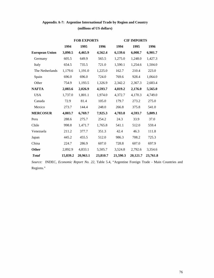
Appendix A-7: Argentine International Trade by Region and Country
(millions of US dollars)
FOB EXPORTS CIF IMPORTS
1994 1995 1996 1994 1995 1996
European Union 3,890.5 4,465.9 4,562.4 6,139.6 6,008.7 6,901.7
Germany 605.5 649.9 565.5 1,275.0 1,248.0 1,427.3
Italy 654.5 735.5 721.0 1,590.1 1,254.6 1,504.0
The Netherlands 1,179.6 1,191.0 1,225.0 162.7 210.4 223.0
Spain 696.0 696.0 724.0 769.6 928.4 1,064.0
Other 754.9 1,193.5 1,326.9 2,342.2 2,367.3 2,683.4
NAFTA 2,083.6 2,026.9 4,593.7 4,819.2 2,176.0 5,565.0
USA 1,737.0 1,801.1 1,974.0 4,372.7 4,170.3 4,749.0
Canada 72.9 81.4 105.0 179.7 273.2 275.0
Mexico 273.7 144.4 248.0 266.8 375.8 541.0
MERCOSUR 4,803.7 6,769.7 7,925.3 4,783.8 4,593.7 5,809.1
Peru 288.6 275.7 254.2 24.3 33.9 37.0
Chile 998.8 1,471.7 1,765.8 541.1 512.0 559.4
Venezuela 211.2 377.7 351.3 42.4 46.3 111.8
Japan 445.2 455.5 512.0 986.3 708.2 725.3
China 224.7 286.9 607.0 728.8 607.0 697.9
Other 2,892.9 4,833.1 5,505.7 3,524.8 2,792.6 3,354.6
Total 15,839.2 20,963.1 23,810.7 21,590.3 20,121.7 23,761.8
Source: INDEC, Economic Report No. 22, Table 5.4, “Argentine Foreign Trade - Main Countries and
Regions.”
76

Appendix A-8: Argentine Exports by Commodity in the Harmonized Tariff Schedule (millions of US dollars)
Item 1989 1990 1991 1992 1993 1994 1995 1996 Primary Products 2,044.5 3,339.1 3,301.2 3,500.2 3,270.9 3,735.3 4,815.9 5,817.1 Live Animals 8.1 8.5 8.4 8.7 13.2 51.0 97.8 44.6 Unprocessed Fish and Shell Fish
258.6 299.7 199.9 321.4 427.3 439.3 498.1 609.2
Honey 23.4 30.8 42.9 51.8 50.1 53.8 70.5 90.6 Unprocessed Vegetables, Legumes
97.3 177.7 192.3 168.2 185.5 259.2 268.4 270.5
Fresh Fruits 151.9 204.3 262.2 286.1 215.4 243.8 417.0 475.5 Cereals 1,015.7 1,374.1 1,066.7 1,547.7 1,453.6 1,332.7 1,862.6 2,560.1 Oil seeds and Fruits 211.4 827.7 4,593.7 790.1 2,176.0 951.8 884.6 963.7 Unprocessed tobacco 56.4 95.0 136.6 142.7 117.0 88.8 100.8 146.0 Raw Wool 65.9 93.6 54.8 41.2 49.1 74.6 86.2 64.7 Cotton fiber 86.3 164.1 202.8 76.6 25.7 176.3 432.8 497.0 Other Primary Products 69.5 63.6 53.4 65.7 37.5 64.0 97.1 95.2 Manufactures of Agricultural Origin
4,005.6 4,663.9 4,927.4 4,829.4 4,932.3 5,805.9 7,473.7 8,439.3
Meat 716.3 873.2 892.0 767.2 748.2 918.1 1,229.1 1,073.5 Processed Fish and Shellfish 22.5 15.4 246.2 236.6 279.3 285.8 416.2 394.9 Dairy Products 137.0 125.1 67.5 35.2 75.8 135.3 260.1 280.6 Other Products of Animal Origin
8.9 9.7 9.5 9.8 12.4 17.3 16.4 21.8
Dry or Frozen Fruits 16.8 20.9 23.2 23.7 21.9 32.0 27.8 33.4 Tea, Yerba Mate, Spices, etc. 42.2 50.3 45.0 46.9 62.3 61.0 67.3 64.6 Milled Products 33.4 65.5 73.4 51.4 59.3 87.8 90.2 166.0 Fats and Oils 875.9 1,151.3 1,221.0 1,109.1 1,078.6 1,533.6 2,097.1 1,890.5 Processed Legumes and Vegetables
159.7 213.1 199.0 260.4 166.4 160.1 321.2 400.1
Beverages, Alcoholic Liq. and Vinegar
40.9 66.0 58.0 64.0 64.2 79.8 165.2 153.1
in German marks) corresponding to the 1992 Financing Plan, which are
1,334.8 1,199.8 1,270.0 1,459.3 1,451.0 1,348.5 1,254.3 2,366.7
Collateralized Tanning and Drying Extracts 39.1 38.5 42.1 40.3 44.2 43.2 39.6 41.4 Skins and Hides 373.9 487.9 513.6 475.1 617.8 762.8 937.0 889.3 Processed Wool 92.7 110.4 86.8 92.1 95.8 113.2 115.5 121.1 Other MAO 49.0 85.9 106.0 92.9 111.8 168.7 314.7 397.8 Source: INDEC, Economic Report No. 22, Table 5.1, “Exports by Item in the Tariff Schedule.”
77

Appendix A-9: Argentine Exports by Commodity in the Harmonized Tariff Schedule
(continued)
(millions of US dollars)
Item 1989 1990 1991 1992 1993 1994 1995 1996
Manufactures of
Industrial Origin
3,185.9 3,364.3 2,983.5 2,823.4 3,678.9 4,646.8 6,504.1 6,465.7
Chemicals and Related Products 487.4 522.5 503.7 533.4 558.8 727.5 972.5 980.0
Artificial Plastic Materials 170.2 171.1 145.8 147.9 132.9 180.6 340.7 339.8
Rubber and its manufactures 72.1 79.5 47.7 39.8 54.7 82.0 128.8 129.6
Leather goods 64.6 69.6 77.3 78.8 118.3 156.6 138.0 146.7
Paper, Cardboard, Printing and
Publications
116.4 153.0 112.6 127.3 149.7 202.3 413.6 377.7
Textiles and Garments 205.0 212.5 147.9 121.6 164.9 210.1 383.8 304.5
Footwear and its Components 40.9 49.2 59.5 51.6 92.3 86.8 102.4 72.7
Stone, Gypsum and Ceramic
Manufactures
72.6 94.1 78.6 71.2 78.8 70.9 109.8 106.7
Precious Stones and Metals and
their Manuf.
2.1 2.2 4.3 4.2 51.9 251.6 23.1 4.9
Base metals and their
manufactures
1,238.6 1,163.3 912.4 643.6 702.5 759.7 1,214.3 1,190.3
Machines and Devices, Electric
Material
430.0 485.7 561.9 518.4 754.8 866.5 983.0 961.5
Transport Material 190.1 223.1 266.3 404.8 719.4 918.2 1,307.8 1,641.9
Other MIO 95.9 138.5 65.5 80.8 99.9 134.0 386.3 209.4
Fuels and Energy 343.3 985.2 765.7 1,081.9 1,235.6 1,651.2 2,169.4 3,088.6
TOTAL 9,579.3 12,352.5 11,977.8 12,234.9 13,117.7 15,839.2 20,963.1 23,810.7
Source: INDEC, Economic Report No. 22, Table 5.1, “Exports by Item in the Tariff Schedule.”
78
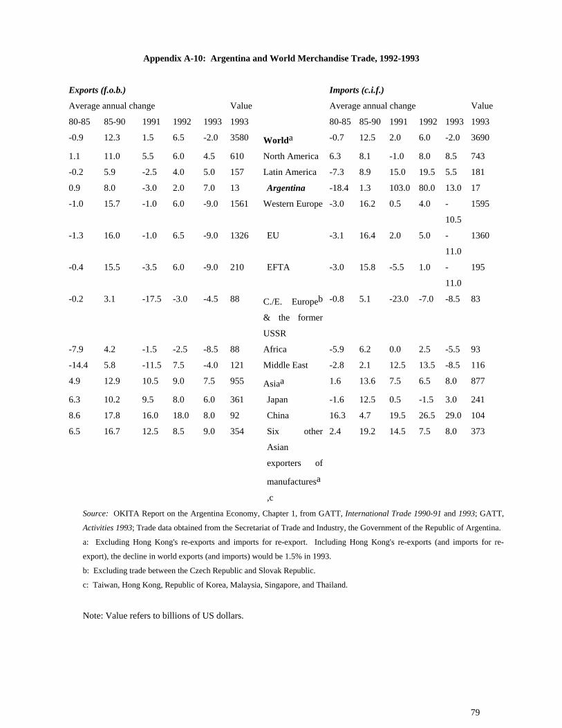
Appendix A-10: Argentina and World Merchandise Trade, 1992-1993
Exports (f.o.b.) Imports (c.i.f.)
Average annual change Value Average annual change Value
80-85 85-90 1991 1992 1993 1993 80-85 85-90 1991 1992 1993 1993
-0.9 12.3 1.5 6.5 -2.0 3580 Worlda -0.7 12.5 2.0 6.0 -2.0 3690
1.1 11.0 5.5 6.0 4.5 610 North America 6.3 8.1 -1.0 8.0 8.5 743
-0.2 5.9 -2.5 4.0 5.0 157 Latin America -7.3 8.9 15.0 19.5 5.5 181
0.9 8.0 -3.0 2.0 7.0 13 Argentina -18.4 1.3 103.0 80.0 13.0 17
-1.0 15.7 -1.0 6.0 -9.0 1561 Western Europe -3.0 16.2 0.5 4.0 -
10.5
1595
-1.3 16.0 -1.0 6.5 -9.0 1326 EU -3.1 16.4 2.0 5.0 -
11.0
1360
-0.4 15.5 -3.5 6.0 -9.0 210 EFTA -3.0 15.8 -5.5 1.0 -
11.0
195
-0.2 3.1 -17.5 -3.0 -4.5 88 C./E. Europeb
& the former
USSR
-0.8 5.1 -23.0 -7.0 -8.5 83
-7.9 4.2 -1.5 -2.5 -8.5 88 Africa -5.9 6.2 0.0 2.5 -5.5 93
-14.4 5.8 -11.5 7.5 -4.0 121 Middle East -2.8 2.1 12.5 13.5 -8.5 116
4.9 12.9 10.5 9.0 7.5 955 Asiaa 1.6 13.6 7.5 6.5 8.0 877
6.3 10.2 9.5 8.0 6.0 361 Japan -1.6 12.5 0.5 -1.5 3.0 241
8.6 17.8 16.0 18.0 8.0 92 China 16.3 4.7 19.5 26.5 29.0 104
6.5 16.7 12.5 8.5 9.0 354 Six other
Asian
exporters of
manufacturesa
,c
2.4 19.2 14.5 7.5 8.0 373
Source: OKITA Report on the Argentina Economy, Chapter 1, from GATT, International Trade 1990-91 and 1993; GATT,
Activities 1993; Trade data obtained from the Secretariat of Trade and Industry, the Government of the Republic of Argentina.
a: Excluding Hong Kong's re-exports and imports for re-export. Including Hong Kong's re-exports (and imports for re-
export), the decline in world exports (and imports) would be 1.5% in 1993.
b: Excluding trade between the Czech Republic and Slovak Republic.
c: Taiwan, Hong Kong, Republic of Korea, Malaysia, Singapore, and Thailand.
Note: Value refers to billions of US dollars.
79

Appendix A-11: Argentine Trade with Mercusor
By Commodity in the Harmonized Tariff Schedule
(millions of US dollars)
FOB Exports CIF Imports
1994 1995 1996 1994 1995 1996
Live animals and animal
products
318.4 553.4 511.6 113.9 72.5 142.3
Vegetable Products 1,044.0 1,310.6 1,405.1 98.2 134.5 134.6
Oils and fats 167.9 144.8 117.8 6.6 13.0 14.9
Foodstuffs 205.6 382.8 427.2 234.9 227.3 174.2
Mineral products 794.8 965.9 1,571.6 250.5 302.3 360.2
Chemicals 353.8 450.5 498.6 454.3 601.4 653.2
Artificial plastic
material
163.9 271.2 301.0 347.3 382.9 454.6
Furs, leather and their
manufactures
138.6 138.8 125.3 6.9 7.0 15.6
Paper 61.4 165.4 184.1 214.7 257.6 326.3
Textile materials and
manufactures
236.9 346.4 429.6 231.0 235.6 355.6
Stone and analog
manufactures
33.8 51.1 43.5 70.8 69.5 90.8
Base metals 91.7 166.1 180.2 508.0 503.8 534.8
Electrical machines and
devices
365.3 576.2 577.1 829.2 787.3 1,088.5
Transport material 770.5 1,121.0 1,396.7 1,228.6 836.9 1,221.8
Other 57.1 125.4 155.9 188.4 162.0 241.7
Total 4,803.7 6,769.6 7,925.3 4,783.8 4,593.7 5,809.1 Source: INDEC, Economic Report No. 22, Table 5.5, “Argentine Foreign Trade with Mercosur.”
80

Bibliography
Agosin, Manuel, 1997. “La insercion internacional de la economia chilena: limites y
oportundades,” CEPRI, Santiago, Chile.
Agosin, Manuel, 1997a. “Un Modelo De Proyeccion de Largo Plazo Para La Economia
Chilena,” Santiago, Chile.
Alvarez, Roberto, 1996. “Beneficios y Costos de un Acuerdo de Libre Comercio con la
Union Europea,” Documento de Trabajo No. 143, Departmento de Economia,
Universidad de Chile, Septiembre.
Amjadi, Azita, and L. Alan Winters, 1997. Transport Costs and “Natural” Integration in
Mercosur, World Bank Policy Research Working Paper 1742, World Bank International
Economics Department, Washington, DC.
Asian Pacific Economic Cooperation, 1997 APEC Economic Outlook, Singapore: APEC.
Butlemann, Andrea and Patricio Meller, “Evaluation of a Chile-U.S. Free Trade
Agreement,” in Economic Commission for Latin America, Trade Liberalization in the
Western Hemisphere, ECLAC: Washington, DC.
Dornbusch, Rudiger and Sebastian Edwards, 1994. “Exchange Rate Policy and Trade
Strategy,” in Bosworth, Barry P., et al. (eds.) The Chilean Economy: Policy Lessons and
Challenges, The Brookings Institution: Washington, DC.
Desormeaux, Jorge, 1995. “Economic Scenarios for Chile,” working paper, Pontificia
Universidad Catolica de Chile.
Donoso, B. and Dominique Hachette, “Mercosur y la apertura comercial chilena,” paper
presented to the Chilean Senate, unpublished manuscript, Department of Economics,
Catolica University, Santiago, Chile.
81

DRI, 1997. World Market Executive Overview, 3rd Quarter.
Economist Intelligence Unit, 1997. Chile: Country Report, 4th Quarter, EIU: London.
Economist Intelligence Unit, 1997. Chile: Country Profile, 1996-1997, EIU: London.
Economist Intelligence Unit, 1997. Argentina: Country Report, 4th Quarter, 1997, EIU:
London.
Economist Intelligence Unit, 1997. Argentina: Country Profile, 1996-1997, EIU:
London.
Harberger, Arnold C., 1996. “Reflections on Economic Growth in Asia and the Pacific,”
Journal of Asian Economics, 7(3): 365-392.
Harrison, Glenn W., Thomas F. Rutherford, and David G. Tarr, 1997. “Trade Policy
Options for Chile,” World Bank Policy Research Working Paper 1783.
International Monetary Fund, 1997. International Financial Statistics, December,
Washington, DC: IMF.
International Monetary Fund, 1997. Direction of Trade Statistics, Washington, DC: IMF.
International Monetary Fund, 1997. World Economic Outlook, Washington, DC: IMF.
Kotabe, Masaaki, 1996. Mercosur and Beyond: The Imminent Emergence of the South
American Markets, Austin, TX: University of Texas at Austin.
Marfan, Manuel and Barry P. Bosworth, 1994. “Saving, Investment, and Economic
Growth,” in Bosworth, Barry P., et al. (eds.) The Chilean Economy: Policy Lessons and
Challenges, The Brookings Institution: Washington, DC.
82

Muchnik, Eugenia; L.F. Errazuriz, and J.I. Dominguez, 1996. “Efectos de la asociation de
Chile as Mercosur en el sector agricola y agroindustrial,” Estudios Publicos, 63: 113-164.
OKITA Foundation, 1996. “OKITA Final Report - Toward a Greater Interdependence
between Argentina and Japan: A New Opportunity for the Argentine Economy,”
conducted by the Japanese International Cooperation Agency, June 1996.
Pacific Economic Cooperation Council, 1997. Pacific Economic Outlook 1997-1998,
Singapore.
Rajapitrana, Sarath, 1996. “Post Trade Liberalization Policy and Institutional Challenges
in Latin America and the Caribbean,” World Bank Working Paper.
Robles, Edgar, 1997. An Exploration into the Sources and Causes of Economic Growth in
the United States and Fourteen Latin American Countries,” Ph.D. Dissertation,
University of California, Los Angeles.
The Undersecretariat of Macroeconomic Planning, 1997. Economic Report No. 22: The
Argentine Economy in the Second Quarter of 1997, Ministry of the Economy: Buenos
Aires.
WEFA, 1997. Asian Economic Outlook, August.
World Bank, 1996. Trends in Developing Countries 1996, Washington, DC: The World
Bank.
Yeats, Alexander J., 1997. “Does Mercosur’s Trade Performance Raise Concerns About
the Effects of Regional Trade Arrangements?” World Bank Policy Research Working
Paper 1729, World Bank International Trade Department, Washington, DC.
83
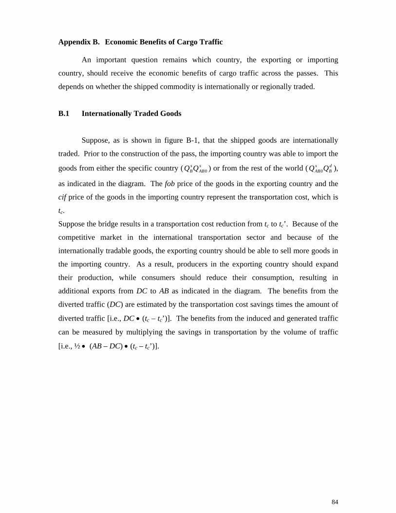
Appendix B. Economic Benefits of Cargo Traffic
An important question remains which country, the exporting or importing
country, should receive the economic benefits of cargo traffic across the passes. This
depends on whether the shipped commodity is internationally or regionally traded.
B.1 Internationally Traded Goods
Suppose, as is shown in figure B-1, that the shipped goods are internationally
traded. Prior to the construction of the pass, the importing country was able to import the
goods from either the specific country ( ) or from the rest of the world ( ),
as indicated in the diagram. The fob price of the goods in the exporting country and the
cif price of the goods in the importing country represent the transportation cost, which is
t
sAB
sBQQ 0
dB
sAB QQ 0
c.
Suppose the bridge results in a transportation cost reduction from tc to tc’. Because of the
competitive market in the international transportation sector and because of the
internationally tradable goods, the exporting country should be able to sell more goods in
the importing country. As a result, producers in the exporting country should expand
their production, while consumers should reduce their consumption, resulting in
additional exports from DC to AB as indicated in the diagram. The benefits from the
diverted traffic (DC) are estimated by the transportation cost savings times the amount of
diverted traffic [i.e., DC • (tc – tc’)]. The benefits from the induced and generated traffic
can be measured by multiplying the savings in transportation by the volume of traffic
[i.e., ½ • (AB – DC) • (tc – tc’)].
84

Figure B-1: INTERNATIONALLY TRADED GOODS
AD
sAQ 0
sAQ 1
dAQ 1
dAQ 0 Q
P
wBB Pcif =
AS
'cA tS +
cA tS +
'ct
ct
BD
BS
BAS +
'BAS +
sBQ s
ABQ 0sABQ 1
dBQ Q
P
A B
CD
ECONOMIC IMPACTS OF TRANSPORTATION COST REDUCTION
EXPORTING COUNTRY IMPORTINGCOUNTRY
xAQ 0xAQ 1
xA
mB QQ 00 =
xA
mB QQ 11 =
11 AA Pfob =
00 AA Pfob =
NET GAINS IN EXPORTING COUNTRY: ABCDNET GAINS IN IMPORTING COUNTRY: NIL
Figure B-2: REGIONALLY TRADED GOODS
AD
sAQ 0
sAQ 1
dAQ 1
dAQ 0
Q
P
AS
'cA tS +
cA tS +
BD
BS
BAS +
'BAS +
sBQ 0
dBQ 0
Q
P
A BCD
E F
ECONOMIC IMPACTS OF TRANSPORTATION COST REDUCTION
EXPORTING COUNTRY
dBQ 1
11 BB Pcif =
IMPORTINGCOUNTRY
HG
11 AA Pfob =
xAQ 0
xAQ 1
xA
mB QQ 00 =
xA
mB QQ 11 =
sBQ 1
'ctct
NET GAINS IN EXPORTING COUNTRY: ABCDNET GAINS IN IMPORTING COUNTRY: EFGH
00 BB Pcif =
00 AA Pfob =
85

B.2 Regionally Traded Goods
As shown in figure B-2, regionally traded shipped goods are solely imported from
one country. This means that the amount of exports in the exporting country (DC) equals
the amount of imports in the importing country (EF). When the transportation costs
decline from tc to tc’, the supply curve of the exported goods inclusive of transportation
costs shifts rightward from SA + tc to SA + tc’ in the exporting country. Accordingly, the
initial supply of the goods in the importing country increases by the same amount,
moving from SA+B to SA+B’. However, both the excess demand for imports in the
importing country and the excess supply of exports in the exporting country determine
the final equilibrium prices for the goods in both countries. At equilibrium, the amount
of exports should increase from DC to AB, while the amount of imports should also
increase from EF to HG. In this scenario, both countries should share the benefits of the
transportation cost reduction, depending upon the supply elasticity of exports and the
demand elasticity for imports.
Mathematically, the share of benefits received by the importing country can be
calculated as follows:
Dm
Sx
Sx
ηεε−
(B-1)
where : Elasticity of supply for exports S
xε : Elasticity of demand for imports D
mη
Elasticity of excess demand for importing country:
m
SS
m
DTDD
m QQ
QQ 0
0εηη −= (B-2)
where : Elasticity of demand for imports Dmη
: Elasticity of demand for importable goods Dη : Elasticity of other suppliers S
0εDTQ :Total demand in importing country sQ0 : Total supply from sources other than particular exporting country
mQ : Quantity of imports
86
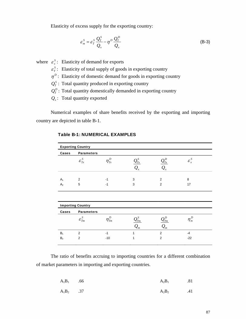
Elasticity of excess supply for the exporting country:
x
DTD
x
STS
TSm Q
QQQ ηεε −= (B-3)
where : Elasticity of demand for exports S
xε : Elasticity of total supply of goods in exporting country S
Tε : Elasticity of domestic demand for goods in exporting country Dη : Total quantity produced in exporting country S
TQ : Total quantity domestically demanded in exporting country D
TQ : Total quantity exported xQ
Numerical examples of share benefits received by the exporting and importing
country are depicted in table B-1.
Table B-1: NUMERICAL EXAMPLES
Exporting Country
Cases Parameters S
Txε DTxη
x
STx
x
DTx
Sxε
A1 2 -1 3 2 8 A2 5 -1 3 2 17
Importing Country
Cases Parameters S
Tmε DTmη
m
STm
m
DTm
Dmη
B1 2 -1 1 2 -4 B2 2 -10 1 2 -22
The ratio of benefits accruing to importing countries for a different combination
of market parameters in importing and exporting countries.
A1B1 .66 A2B1 .81 A1B2 .37 A2B2 .41
87

Appendix C. The Economic Cost of Foreign Exchange
C.1 Introduction
The foreign exchange premium in Argentina is expected to decline because future
trade policy is geared toward further trade liberalization in the Mercosur Region and with
the rest of the world. The direction of the foreign exchange premium in Chile, on the
other hand, should depend upon future trade and tax policies.
C.2 Background
When a project demands additional foreign exchange, it exerts depreciating
pressure on the value of the domestic currency. Some importers react by cutting back
their demand for imported goods, while exporters increase their supply of exports. In the
end, the project’s use of foreign exchange is usually met partly by a cutback in demand
and partly by additional supply.30
Since the demand for imported goods is generally distorted by import tariffs, as is
the supply by subsidies and export taxes, there should be a difference between the
economic price of foreign exchange and the market exchange rate. This difference
should represent the loss of tariff revenues associated with foregone imports, as well as
other distortions associated with additional production of exported goods in the external
sector.
A further distortion must be considered in the area of domestic sales taxes. While
the demand for imports is expected to decline because of additional demand for foreign
exchange and the resulting devaluation of the domestic currency, the domestic sales taxes
associated with these goods should also be foregone. On the supply side, the resources
required to produce additional exports have to come from the non-traded goods sector,
which reduces the supply of and the corresponding demand for non-traded goods and the
30 A.C. Harberger, “Survey of Literature on Cost-Benefit Analysis for Industrial Project Evaluation”, Project Evaluation -- Collected
Papers, (Chicago: the University of Chicago Press, 1972), Chapter 2.
88

associated VAT and other sales tax revenues. All these repercussions in the economy
have to be accounted for as part of the foreign exchange premium.
The above analysis concerns the foreign exchange needed for the project and its
impact on the non-traded goods sector in the economy. The reverse also holds if the
project generates foreign exchange. Therefore, a foreign exchange premium must be
applied to the foreign exchange component of the goods demanded or supplied by the
project in the economic analysis. This adjustment ensures that the project’s use or
generation of foreign exchange adequately reflects the economic opportunity cost of
foreign exchange in the country.
C.3 Methodology
The economic price of foreign exchange is measured by the value of the unit of
foreign exchange relative to the economy in terms of domestic resource costs. The extent
to which the economic cost of foreign exchange exceeds the free market foreign
exchange rate is termed the foreign exchange premium.
The foreign exchange premium is composed of two components. The first is the
distortion caused directly in the external trade sector. This is calculated by taking the
weighted average of the value of foregone imports and the cost of resources used to
produce additional exports. The value of imported goods to demanders can be measured
by the c.i.f. prices plus tariffs -- the demand curve D’ as illustrated in Figure C-131--
while the resource cost of producing exports is measured by the f.o.b. prices minus export
taxes plus export subsidies -- the supply curve S’.
For convenience, we choose the units of the goods so that the initial supply prices
of importable goods (Pm), exportable goods (PX), and non-traded goods (Pnt), are equal to
one. That is, Pm = Px = Pnt = 1. Thus, the quantities demanded or supplied are equal to
their values.
89

The market exchange rate (Em) is determined by the demand curve for imports
exclusive of tariffs and the supply of exports inclusive of export subsidies and exclusive
of export taxes. When foreign goods are imported for use in a project (Q1 – Q2), the
demand curve for foreign exchange is shown as a shift to the right from D to D* in Figure
C-1. The economic value of foreign exchange is, in turn, determined by the value of
imported goods inclusive of tariffs and the resource cost of producing all exported goods
exclusive of export subsidies but inclusive of export taxes. At the margin, the excess
amount of economic value over the market value represents the first component of the
foreign exchange premium (ρ1), which is indicated as the shaded area in Figure C-1. This
can also be expressed mathematically as follows:
idxs tftf ⋅+⋅=1ρ (C-1)
where tx is the weighted average rate of subsidies (in excess of export taxes) on those
exports that are responsive to changes in the exchange rate, ti is the weighted average rate
of import tariffs on those imports that are responsive to changes in the exchange rate, fs
and fd are the weights on the supply and demand sides, respectively.
The weights, fs and fd, depend upon the demand elasticities of imports, the supply
elasticities of exports, and other factors. The above formula can then be re-written as:
( )( )xi
dsixi
dx
s
qqtqqt
ηεηε
ρ−−⋅
=1 (C-2)
where εs is the supply elasticity of exports and ηd is the demand elasticity for imports, qi
is the quantity of foreign exchange required to pay for imports, and qx is the quantity of
foreign exchange earned from exports.
31 See G.P. Jenkins and A.C. Harberger, Cost-Benefit Analysis of Investment Decisions, Harvard Institute for International
90

Figure C-1: DETERMINATION OF ρ1The second component of the foreign exchange premium is measured by the effect of the
VAT and other sales taxes on the economic price of foreign exchange. When foreign exchange is needed in a project, the market exchange rate goes up from Em to Em
’ as was previously mentioned. Given that the country is a small open economy, this raises the prices of importable and exportable goods expressed in domestic currency (from P0 to P1 for the net-of-tax price, and Pv
0 to Pv1 for the gross-of-tax price as shown in Figures C-2A
and C-2B). Two events should then occur in the economy.
D
S
mE
'mE
ExchangeRate
D*
D'
S'
Quantity ofForeign Exchange
0Q 1Q2Q
First, the quantity of importable goods demanded should decline from dMQ 0 to
dMQ 1 and the quantity of importable goods supplied should go up from s
MQ 0 to sMQ 1.
Accordingly, the excess demand for importable goods should be reduced from sMQ 0
dMQ 0
to sMQ 1
dMQ 1 (Figure C-2A).
A similar situation is expected to take place in the exportable goods sector. The
quantity demanded should decline, while the quantity supplied should increase. The net
excess supply of exportable goods should increase from dXQ 0
sXQ 0 to d
XQ 1sXQ 1, as shown
in Figure C-2B.
Additional resources will be required to produce the additional importable and
exportable goods. Given our assumption of full employment, these resources must be
Development, (1997), a manual for Program on Investment Appraisal and Management..
91

released from the non-traded goods sector. Due to increases in the relative prices of
traded goods, the supply of non-traded goods should shift left from SNT to S’NT, as shown
in Figure C-2C. The reduction in the supply of non-traded goods should push up their
net-of-tax prices from P0 to P1. Consequently, the relative ratio of the price of traded to
non-traded goods should be somewhat depressed, inducing a further round of adjustment
in the quantity supplied of importable and exportable goods. These adjustments should
continue at a declining pace until a final equilibrium is re-established. At the new
equilibrium, the total resources released from non-traded goods to the tradable goods
sector should be less than the initial response (shown as *sMQ 1 and *s
XQ 1 instead of sMQ 1
and sXQ 1 in Figure C-2A and 2B). Nevertheless, the resources released from the non-
traded goods sector in equilibrium must meet the demand for additional production of
importable and exportable goods. That is,
(C-3) *10
*100
*1
sX
sX
sM
sM
sNT
sNT QQQQQQ +=
Since the non-traded goods are also subject to VAT and other indirect taxes, the taxes
associated with the reduction of demand from QdNT0 to Qd
NT1 will be foregone. The
foregone VAT and other indirect taxes should, therefore, be accounted for as part of the
foreign exchange premium.
In summary, the three shaded areas identified in Figures C-2A, C-2B and C-2C
should be all accounted for by the foreign exchange premium in a general equilibrium
analysis. One can express the impact of additional demand for foreign exchange in a
project on the domestic indirect tax as a combined foregone VAT and other indirect taxes
associated with cutback of the demand for importable, exportable, and non-traded goods.
The weights are the corresponding responses of their demands to the market exchange
rate:
( ) ( ) ( )( ) ( ) ( )md
NTmd
Xmd
M
NTmd
NTXmd
XMmd
M
EQEQEQVEQVEQVEQ
∂∂−∂∂−∂∂−⋅∂∂−⋅∂∂−⋅∂∂−
=2ρ (C-4)
92

Figure C-2: DETERMINATION OF ρ2
D
SM
'P
Price
DV
P
VP0
VP1
sMQ 0
sMQ 1
dMQ 1
dMQ 0
A. Importable
D
SX
'P
Price
DV
P
VP0
VP1
sXQ 0
sXQ 1
dXQ 1
dXQ 0
B. Exportable
D
SNT
Price
DV
0P
VP0
VP1
sNT
dNTQ
Q0
0=
C. Non-Tradable
S'NT
1P
*1
1sNT
dNTQ
Q=
*1
sXQ
*1
sMQ
where VX, VM, and VNT are the average VAT and other indirect tax rates for exportable,
importable, and non-tradable goods, respectively.
From equation (C-3), the demand for non-traded goods must be equal to the
supply of non-traded goods in equilibrium, hence QdNT = Qs
NT and ∆QdNT = - ∆Qs
NT. In
addition, if the economy has reached the limits of its production possibilities and there is
no incremental foreign borrowing, the resources released from the non-traded goods
sector must be employed to produce importable and exportable goods. This implies that
the following equation holds:
(C-5) sX
sM
sNT QQQ ∆+∆=∆
93

Given the definition of demand elasticities of importable, exportable and non-
traded goods, ηdM = (∂Qd
M/∂Em)/(QdM /Em), ηd
X = (∂QdX/∂Em)/(Qd
X/Em), and ηdNT =
(∂QdNT/∂Em)/(Qd
NT/Em), equation (C-5) can be rewritten as:
- ηdM•(Qd
M/Em)•VM - ηdX•(Qd
X/Em)•VX - ηdNT•(Qd
NT/Em)•VNT
ρ2 = (C-6) - ηd
M•(QdM/Em) - ηd
X•(QdX/Em) - ηd
NT•(QdNT/Em)
With the multiplication of the numerator and the denominator of the above
equation by (Em/QdT), where Qd
T denotes the demand for the total tradable goods, the
equation can be written as follows:
- ηdM•(Qd
M/QTd)•VM - ηd
X•(QdX/QT
d)•VX - ηdNT•(Qd
NT/QTd)•VNT
ρ2 = (C-7) - ηd
M•(QdM/ QT
d) - ηdX•(Qd
X/ QTd) - ηd
NT•(QdNT/ QT
d)
Let us assume that the effective VAT and other indirect tax rates for the
importable and exportable goods (VM = VX) are equal, as is most likely the case in a
comprehensive tax system. We can then combine the importable and exportable goods in
the total tradable goods sector as follows:
- [ηd
T•QdT•VT] – [ηd
NT•QdNT•VNT]
ρ2 = (C-8) - [ηd
T•QTd] – [ηd
NT•QdNT]
where ηdT and ηd
NT denote the demand elasticities of tradable and non-tradable goods and
QdNT denotes the quantities of demand for non-tradable goods. Thus, ρ2 can be
considered a weighted average of the effective VAT and other indirect tax rates for
tradable and non-traded goods, where the weights are the demand for tradable goods and
non-tradable goods.
While calculating the foreign exchange costs and benefits for a project, one can
combine the above two components, ρ1 and ρ2. Recall that ρ1 is associated with the
amount of foreign exchange acquired for or earned by the project, while ρ2 is related to
94
the corresponding changes in the amount of tradable goods. The amount of foreign
exchange acquired and the corresponding sum of the changes in the demand and supply
of tradable goods are equal. Therefore, ρ1 and ρ2 can both be applied to the amount of
foreign exchange acquired or earned by the project in question. Estimating the foreign
exchange premium in this way is an approximation to a general equilibrium estimation of
the foreign exchange premium.
C.4 Empirical Estimation
We first estimate the foreign exchange premiums for Argentina and Chile using
the 1995 structure of the economy and taxes. We then take into account the expected
impact of future changes in trade distortions and the VAT induced by the MERCOSUR
Treaty for Argentina and by free trade with MERCOSUR or with NAFTA (for Chile).
The Current Foreign Exchange Premium
Argentina
In order to calculate the effective import tariff rates, one has to exclude re-exported
imports. For Argentina, 10% of exports are assumed to be re-exported imports. No really
reliable data is available for Argentina, but 10% appears to be the general experience in
similar countries.
The government’s purchase of goods and services is generally subject to import
tariffs in the same manner as the private sector. However, since there is no data on the
breakdown of customs duties paid on public and private purchases, it is assumed that
public purchases are also responsive to changes in market exchange rates.
Using the 1995 import tariffs, export taxes, and economic structure, the data, expressed in
millions of pesos, are presented for Argentina as follows:32
32 See International Monetary Fund, International Financial Statistics, (August 1997), National Accounts of Argentina. The data on
imports are inclusive of customs duties.
95
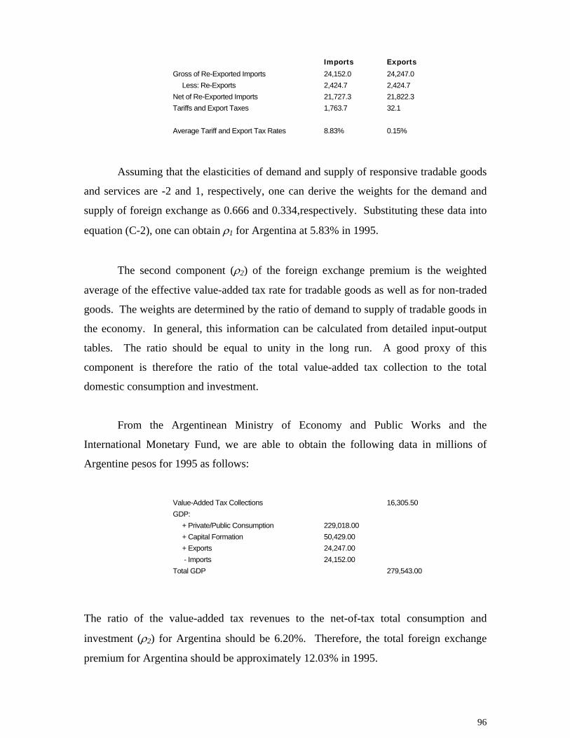
Imports Exports Gross of Re-Exported Imports 24,152.0 24,247.0 Less: Re-Exports 2,424.7 2,424.7 Net of Re-Exported Imports 21,727.3 21,822.3 Tariffs and Export Taxes 1,763.7 32.1 Average Tariff and Export Tax Rates 8.83% 0.15%
Assuming that the elasticities of demand and supply of responsive tradable goods
and services are -2 and 1, respectively, one can derive the weights for the demand and
supply of foreign exchange as 0.666 and 0.334,respectively. Substituting these data into
equation (C-2), one can obtain ρ1 for Argentina at 5.83% in 1995.
The second component (ρ2) of the foreign exchange premium is the weighted
average of the effective value-added tax rate for tradable goods as well as for non-traded
goods. The weights are determined by the ratio of demand to supply of tradable goods in
the economy. In general, this information can be calculated from detailed input-output
tables. The ratio should be equal to unity in the long run. A good proxy of this
component is therefore the ratio of the total value-added tax collection to the total
domestic consumption and investment.
From the Argentinean Ministry of Economy and Public Works and the
International Monetary Fund, we are able to obtain the following data in millions of
Argentine pesos for 1995 as follows:
Value-Added Tax Collections 16,305.50 GDP: + Private/Public Consumption 229,018.00 + Capital Formation 50,429.00 + Exports 24,247.00 - Imports 24,152.00 Total GDP 279,543.00
The ratio of the value-added tax revenues to the net-of-tax total consumption and
investment (ρ2) for Argentina should be 6.20%. Therefore, the total foreign exchange
premium for Argentina should be approximately 12.03% in 1995.
96

Chile
There are no taxes on exports in Chile. From data33 on imports summarized in
Table C-1 and assuming that 10% of gross imports in Chile are re-exported, our
calculations show that the average import tariff in Chile ranged between 9% and 10%
from 1990-1995, while the statutory uniform tariff rate in Chile was 11%.
Table C-1: Imports in Billion Chilean Pesos (1990-1995)
1990 1991 1992 1993 1994 1995 Gross Imports 2874.7 3467.7 4390.3 5334.7 5866.7 7304.4 Less Re- Exports
319.36 394.29 461.55 491.62 618 781.22
Net Imports 2555.34 3073.41 3928.75 4843.08 5248.7 6523.18 Imports Duties 222.49 276.26 334.83 413.11 429.27 535.55 Average Tariff 9.54% 9.88% 9.32% 9.33% 8.91% 8.94%
If we assume that the elasticities of demand and supply of responsive tradable goods and
services are -2 and 1, respectively, we can first calculate the weights on demand and
supply of foreign exchange and then substitute these weights into equation (C-2) to
obtain ρ1 for Chile for each year of the period 1990-1995 (see Table C-2).
Table C-2: First Component of Foreign Exchange Premium
1990 1991 1992 1993 1994 1995
Supply Elasticity of Exports 1 1 1 1 1 1 Demand Elasticity of Imports -2 -2 -2 -2 -2 -2 Quantity of Foreign Exchange to pay for Imports (billion Ps)
2555.34 3073.41 3928.75 4843.08 5248.7 6523.18
Quantity of Foreign Exchange to pay for Export (billion Ps)
2874.24 3548.61 4153.95 4424.58 5562 7030.98
ρ1 6.10% 6.26% 6.09% 6.40% 5.82% 5.81%
The second component (ρ2) of the foreign exchange premium is the weighted
average of the effective VAT and other indirect taxes on tradable goods as well as non-
traded goods. If we assume that the elasticities of demand and supply of tradable goods
are approximately equal, and that the quantities of traded goods demanded and supplied
are equal, then ρ2 can be estimated simply as the ratio of the total indirect tax collections
to the total domestic consumption and investment.
33 See International Monetary Fund, International Financial Statistics Yearbook, (1997), National Accounts of Chile. The data on
imports are inclusive of customs duties.
97

Table C-3: Second Component of Foreign Exchange Premium
1990 1991 1992 1993 1994 1995
Taxes*: General Sales Taxes Turnover or VAT
649.83 932.83 1268.37 1558.4 1831.18 2128.19
Total 649.83 932.83 1268.37 1558.4 1831.18 2128.19 Expenditures*: Private Consumption 5609.1 7450.3 9664.2 11777.8 13692.8 16550.9 Public Consumption 906.2 1146.9 1457.4 1788.1 2041 2338 Gross Fixed Capital Formation
2158.9 2510.1 3517 4715.3 5321.9 6206.5
Total 8674.2 11107.3 14638.6 18281.2 21055.7 25095.4
ρ28.10% 9.17% 9.49% 9.32% 9.53% 9.27%
*Taxes and expenditures in billion Pesos
The foreign exchange premium ρ is the sum of ρ1 and ρ2. For Chile, the second
component is, on the average, greater than the first component, reflecting a uniform and
low import tariff rate combined with a high and comprehensive VAT system. The total
foreign exchange premium for Chile was approximately 15% in 1995.
1990 1991 1992 1993 1994 1995
ρ1 6.10% 6.26% 6.09% 6.40% 5.82% 5.81%
ρ2 8.10% 9.17% 9.49% 9.32% 9.53% 9.27% Foreign Exchange Premium 14.20% 15.43% 15.58% 15.72% 15.35% 15.08%
The Foreign Exchange Premium in Future Years
The Mercosur Treaty will reduce import tariffs and consequently lower future
foreign exchange premiums in Argentina. Foreign exchange premiums in Chile in the
future should depend upon future trade and tax policies.
Argentina
Trade between Argentina and members inside or outside Mercosur should reduce
import duty rates in the future. From Table C-4 it is clear that the speed of reduction
should be much faster within the Mercosur region. In 1995, about 26% of total imports
98

came from Mercosur. With a faster tariff rate reduction in the Mercosur region in
foreseeable future, we assume that for the purpose of this project, 30% of the total
imports should come from Mercosur member countries and the remainder from the rest
of the world. One can deduce from the tariff schedules that import tariff rates should be
reduced approximately 7% per year from 1997 to 1998 and 11% from 1998 to 2001.
This may be a crude estimate, because the weights of imports by commodities and
different proportions of imports from within and outside the Mercosur area are not
properly taken into account.
Table C-4: IMPORT DUTY RATES IN ARGENTINA
1996 1998 2001 Categories Outs Ins Outs Ins Outs Ins Primary Industrial Materials 5.4 2.5 3.4 1.5 2.9 0
Primary Agricultural Materials 8.4 5.4 7.5 3.5 5.4 0
Intermediate Industrial Inputs 14.6 12.6 12.6 8.5 11.5 0
Intermediate Agricultural Inputs 13.5 10.5 12.6 7.5 10.7 0
Capital Goods 13.3 10.3 13.2 7.5 13.2 0
Semi-durable Goods 22.6 19.5 20.6 15.0 18.5 0
Non-durable Goods 16.6 13.5 14.5 10.0 13.6 0
Durable Goods 19.8 16.8 18.8 12.0 16.2 0
We further assume that the export tax and value-added tax in Argentina will
remain unchanged in the future. With the same economic structure today, one can
estimate the foreign exchange premium over the next five years as follows: 1995 1997 1998 1999 2000 2001
ρ1 5.83 5.04 4.68 4.16 3.70 3.29
ρ2 6.20 6.20 6.20 6.20 6.20 6.20
ρ 12.03 11.24 10.88 10.36 9.90 9.49
Chile
A trade policy option for Chile is to join either MERCOSUR or NAFTA. Another
trade policy is to set a complementary tariff reduction with a non-partner in combination
with free trade area options. Under either scenario, the first component of the foreign
exchange premium should fall, because the tariff rate will be reduced. The direction of
the second component of the foreign exchange premium, on the other hand, should
99

depend on the efficiency of indirect tax collection. By reducing the import tariff rate
because of the free trade area, an increase in domestic taxes is required in order to
maximize the benefits from trade reform34. Such an improvement in domestic tax
collection would entail a higher value of the second component of the foreign exchange
premium.
C.5 Concluding Remarks
This appendix has developed a comprehensive framework to measure the foreign
exchange premiums in Argentina and Chile now and in the future. The foreign exchange
premium for Argentina is expected to decline over time because of the Mercosur Treaty
and global trade liberalization.
The extent to which the foreign exchange premium in Chile should change is
expected to depend upon future trade and tax policies. A free trade area with either
MERCOSUR or NAFTA should reduce import tariffs, lowering the foreign exchange
premium and improving the collection rate of VAT, which should increase the foreign
exchange premium. These two opposing effects of future trade liberalization currently
make it difficult to predict the expected direction of the foreign exchange premium in
Chile.
34 Trade Policy Options for Chile: A Quantitative valuation, Gleen Harrison, Thomas Rutherford, and David Tarr (June 1997)
100

Appendix D. The Economic Cost of Labor
D.1 Background
The economic cost of labor (EOCL) used by the project will vary by skill, by
location of employment, and by type of labor market. Unlike capital and foreign
exchange, labor cannot be measured by using a single value to determine economic costs.
It is, therefore, not appropriate to use a single value or a single conversion factor to
represent the economic cost of labor.
D.2 Methodology
We use the private supply price of labor necessary to induce people to work for
the project in question as the fundamental determinant of the economic cost of labor.35 It
is then adjusted for any gain or loss in taxes that accrues to the government. This
includes personal income taxes and social security contributions paid to the government,
exclusive of any direct pension benefits paid to these workers upon their retirement.
This approach takes into account labor’s preferences for the location, working
conditions associated with the project, and environmental characteristics of the project
region. This approach reflects the fact that workers require different levels of wages to
do similar jobs in alternative areas and working conditions.36 For example, if a high
wage rate is required to induce labor to work on a project where the living and working
conditions are harsh and risky, it is this wage rate that should be used as the basis for
estimating the economic cost of labor, not the value of the product foregone from the
previous activity in the economy. On the contrary, if a worker leaves a high-paying job
in a remote and isolated region to take a job in a central city, the economic cost of this
worker would be less than in his previous employment.
35The supply price of labor for a project is the minimum wage rate the project has to pay in order to obtain or attract supplies of
labor with the appropriate skill levels. See A.C. Harberger, “On the Social Opportunity Cost of Labour”, Project Evaluation: Collected Papers, (Chicago: University of Chicago Press, 1972). An alternative approach is to measure the economic cost of labor as the value of the product that is foregone by the economy when a worker accepts a job with the project plus an adjustment to reflect any changes in living and working conditions perceived by the workers.
36 See, e.g., G.P. Jenkins and C.Y. Kuo, “On Measuring the Social Opportunity Cost of Permanent and Temporary Employment”,
Canadian Journal of Economics, (May 1978).
101

Once the minimum supply price of labor has been determined, the EOCL can be
calculated by adjusting that value to account for distortions which may affect the market
wage rate. Using this approach, the net-of-tax wage earned in the competitive market in
the project region can be considered the minimum private supply price.
We are dealing with a competitive market in Argentina and Chile. For the past
five years, wage rates in Argentina have not been controlled by strong unions and
government regulation, but rather have been basically determined by free competitive
markets. In the case of Chile, the competitive markets have existed for two decades.
Thus, the economic cost of labor associated with the incremental demand by the project
in Argentina and Chile (EOCL) can be measured by the weighted average of the market
wage foregone due to the replacement of workers elsewhere and the economic cost of
new labor entering the market.37 This can be written as follows:
nm WWEOCL ⋅+⋅= 21 αα (D-1)
where α1 is the fraction of the incremental demand being met by the workers employed
elsewhere in the economy and α2 is the remaining fraction being met by the net increase
in labor supply. Thus, α1 + α2 = 1. Wm is the market wage and Wn is the net-of-tax
supply price of labor to the job.
Alternatively, equation (D-1) can be re-written as follows:
( )mnm WWWEOCL −+= 2α
tWWEOCL mm ⋅⋅−= 2α (D-2)
37 In a competitive labor market, the marginal value of a unit of a worker’s non-labor market activity will be equal to the after-tax
wage rate he receives from working and the after-tax unemployment insurance benefit, if any.
102

where t is the marginal income tax rate, including the portion of social security
contributions being considered as tax. In other words, the differential between Wm and
Wn represents the externalities generated by workers moving from non-labor market
activity to labor market activity.
D.3 Empirical Estimation
The Andean Highway Pass projects are expected to create a significant number of
construction jobs during the two to three years of the construction period. After the pass
is set in places, some operating and maintenance workers will be required over the life of
the pass. During the construction period, there are three types of workers required for the
project in terms of skill level: unskilled workers, skilled workers, and professionals.
Argentina
The unemployment rate in Argentina has been high over the past five years. The
overall rate was 6.7% in 1992, 10.1% in 1993, 12.1% in 1994, 18.8% in 1995, and 18.4%
in 1996.38 The unemployment rate in the construction sector was even higher, measuring
31.4% in April 1996 and 29.6% in October 1996 in urban areas. This high
unemployment should provide a large proportion of workers from the unemployed pool,
especially unskilled workers. For this exercise, we assume that the proportion hired from
the unemployed pool would be 50% unskilled workers, 40% skilled workers, and 15%
technicians and professionals.
According to equation (D-2), the distortions associated with the labor markets in
Argentina reflect the sum of personal income taxes and social security taxes. The
personal income tax system in Argentina is progressive in nature, ranging from 6% to
33%. For the purpose of this study, the marginal personal income tax rates are estimated
to be 6% for unskilled workers, 10% for skilled workers, and 25% for technicians and
professionals.
38 International Monetary Fund, International Financial Statistics, (August 1997), p. 102.
103
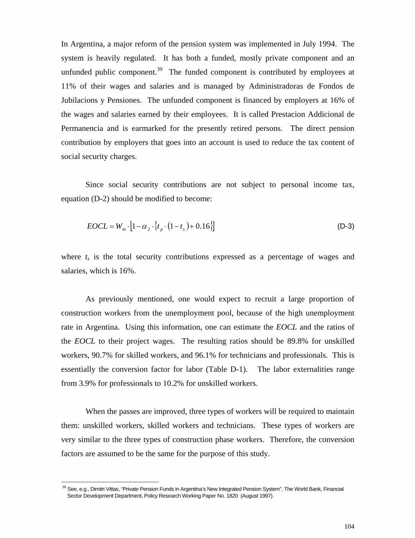
In Argentina, a major reform of the pension system was implemented in July 1994. The
system is heavily regulated. It has both a funded, mostly private component and an
unfunded public component.39 The funded component is contributed by employees at
11% of their wages and salaries and is managed by Administradoras de Fondos de
Jubilacions y Pensiones. The unfunded component is financed by employers at 16% of
the wages and salaries earned by their employees. It is called Prestacion Addicional de
Permanencia and is earmarked for the presently retired persons. The direct pension
contribution by employers that goes into an account is used to reduce the tax content of
social security charges.
Since social security contributions are not subject to personal income tax,
equation (D-2) should be modified to become:
( ){ }[ ]16.011 2 +−⋅⋅−⋅= spm ttWEOCL α (D-3)
where ts is the total security contributions expressed as a percentage of wages and
salaries, which is 16%.
As previously mentioned, one would expect to recruit a large proportion of
construction workers from the unemployment pool, because of the high unemployment
rate in Argentina. Using this information, one can estimate the EOCL and the ratios of
the EOCL to their project wages. The resulting ratios should be 89.8% for unskilled
workers, 90.7% for skilled workers, and 96.1% for technicians and professionals. This is
essentially the conversion factor for labor (Table D-1). The labor externalities range
from 3.9% for professionals to 10.2% for unskilled workers.
When the passes are improved, three types of workers will be required to maintain
them: unskilled workers, skilled workers and technicians. These types of workers are
very similar to the three types of construction phase workers. Therefore, the conversion
factors are assumed to be the same for the purpose of this study.
39 See, e.g., Dimitri Vittas, “Private Pension Funds in Argentina’s New Integrated Pension System”, The World Bank, Financial
Sector Development Department, Policy Research Working Paper No. 1820 (August 1997).
104
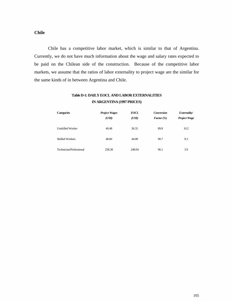
Chile
Chile has a competitive labor market, which is similar to that of Argentina.
Currently, we do not have much information about the wage and salary rates expected to
be paid on the Chilean side of the construction. Because of the competitive labor
markets, we assume that the ratios of labor externality to project wage are the similar for
the same kinds of in between Argentina and Chile.
Table D-1: DAILY EOCL AND LABOR EXTERNALITIES
IN ARGENTINA (1997 PRICES)
Categories Project Wages
(US$)
EOCL
(US$)
Conversion
Factor (%)
Externality/
Project Wage
Unskilled Worker 40.48 36.35 89.8 10.2
Skilled Workers 48.60 44.08 90.7 9.3
Technician/Professional 258.38 248.04 96.1 3.9
105

Appendix E. Eeconomic Costs of Tradable and Non-Tradable Goods
E.1 Economic Cost of Tradable Inputs
The financial cost of each tradable input is the net-of-tax cost adjusted for the
foreign exchange premium. For example, the foreign exchange premium for Chile was
estimated to be 15%. If the financial price of equipment is $1 inclusive of VAT, then the
economic cost of the equipment is estimated to be $0.878, which is calculated by net-of-
tariff (at an 11% rate) and VAT (at an 18% rate) first and then adjusted upward for the
foreign exchange premium (at 15%). That is, 0.878 = [1/(1.11*1.18)]*1.15.
All of the conversion factors for the tradable inputs used in the construction and
operating phases of the passes are calculated. In other words, all the inputs are to be
adjusted for the foreign exchange premium, tariff, excise tax, and VAT.
The conversion factors for diesel fuel and gasoline in Argentina are 0.689 and
0.539 in 1998, respectively. This is based on excise tax rates of 33% for diesel and 70%
for gasoline, as well as the VAT rate of 21%. That is, 0.689 = [1/(1.33*1.21)]*1.1088
and 0.539 = [1/(1.7*1.210]*1.1088.
In the case of Chile, excise taxes are 1.5 UTM (monthly tax unit) per cubic meter
for diesel fuel and 4.4084 UTM per cubic meter for gasoline. The value of 1 UTM is
20,265 Pesos. Thus, the excise taxes expressed in Chilean Pesos are 30,397.5 pesos for
diesel fuel and 89,336.2 pesos for gasoline. By using the tax-inclusive fuel costs for
diesel at $410 per cubic meter and for gasoline at $820 per cubic meter and also using the
exchange rate at 425 Pesos per US dollar, we can derive the equivalent excise rates at
25.9% and 43.4%, respectively (That is, 0.259 = 30,397.5/[(410*425/1.18) – 30,397.5]
and 0.434 = 89,336.2/[(820*425/1.18) – 89,336.2]. We then estimate the conversion
factors for diesel fuel and gasoline at 0.697 (= [1/(1.11*1.259*1.18)]*1.15) and 0.612
(=[1/(1.11*1.434*1.18)]*1.15).
106

E.2 Economic Cost of Non-Tradable Inputs
In the case of non-tradable goods, the economic cost is estimated as a weighted
average of the demand and supply prices of the goods. That is, the economic cost per
unit demanded (Pe) is estimated as a weighted average of the value of the resources used
in the production of the additional supply (Ps) and the value of the consumption foregone
by the existing demand (Pd). The conversion factor (CF) can be measured by the ratio of
(Pe) to the financial cost of the project (P*). These relationships can be expressed as
follows:
Pe = ωd • Pd + ωs • Ps (E-1)
CF = Pe/P* (E-2)
where ωd and ωs are the proportions of the incremental demand for non-tradable good
obtained at the expense of the current demand and the additional supply of the goods; Pd
is the demand price adjusted for VAT, and Ps is the resource cost to produce an additional
unit.
Since Argentina has a large amount of excess capacity in its economy, a greater
weight is placed on supply. For the purpose of this study, two-thirds and one-third are
assumed for both ωs and ωd, respectively. In the case of Chile, we also assume half by
half for demand and supply.
For illustrative purposes, we describe the steps to construct the conversion factor
for Portland Cement in Argentina. The first step is to obtain the detailed breakdown of
financial costs to produce one ton of cement, shown in Column (2) of Table E-1. The
tradable content of each of the input components is identified in Column (3). The
conversion factor for each input component is estimated and presented in Column (4).
The last column shows the economic cost of each input component. Finally, the
economic cost of producing one ton of cement will be 63.09 pesos. According to
equation (E-1), one can calculate the economic price of Portland Cement required for the
107
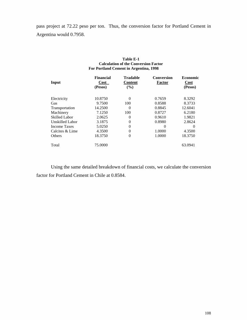
pass project at 72.22 peso per ton. Thus, the conversion factor for Portland Cement in
Argentina would 0.7958.
Table E-1
Calculation of the Conversion Factor For Portland Cement in Argentina, 1998
Financial Tradable Conversion Economic Input Cost Content Factor Cost (Pesos) (%) (Pesos)
Electricity 10.8750 0 0.7659 8.3292 Gas 9.7500 100 0.8588 8.3733 Transportation 14.2500 0 0.8845 12.6041 Machinery 7.1250 100 0.8727 6.2180 Skilled Labor 2.0625 0 0.9610 1.9821 Unskilled Labor 3.1875 0 0.8980 2.8624 Income Taxes 5.0250 0 0 0 Calcites & Lime 4.3500 0 1.0000 4.3500 Others 18.3750 0 1.0000 18.3750 Total 75.0000 63.0941
Using the same detailed breakdown of financial costs, we calculate the conversion
factor for Portland Cement in Chile at 0.8584.
108

Appendix F. The Conversion Factors for Transportation Services
The transportation services of truck and passenger bus are important for this
project. They are, in fact, non-tradable services. By using the same approach and the
same assumptions as outlined in Appendix E, we start with the detailed breakdown of
vehicle operating costs (VOC) per 1000 vehicle-km. The economic cost of producing per
1000 vehicle-km truck services in Argentina would be US$966.75 as shown in Table F-1.
Table F-1
Calculation of the Conversion Factor for Providing 1000 km Truck Services in Argentina, 1998
VOC Financial Tradable Conversion Economic Components Cost Content Factor Cost (dollars) (%) (dollars)
Fuel 229.48 100 0.6890 158.11 Lubricants 34.41 100 0.9164 31.53 Tires 140.63 100 0.7766 109.21 Crew Time 225.32 0 0.9070 204.37 Cargo Holding 10.25 0 1.0000 10.25 Maintenance Labor 82.64 0 0.9070 74.95 Maintenance Parts 152.33 100 0.7968 121.38 Depreciation 135.54 100 0.7330 99.36 Interest 97.59 0 1.0000 97.59 Overhead 60.00 0 1.0000 60.00 Total 1,168.18 966.75 By using equation (E-1) and the current assumptions of the Argentinean economy,
one can calculate the economic price of truck services required for the highway project at
US$1,033.33 per 1,000km. The conversion factor for truck services in Argentina would
be 0.8845.
The same calculation can be performed for Chile. With a tighter economy in
Chile, we assume half by half for demand and supply, ωd and ωs, respectively. The
conversion factor for truck services is 0.8679.
The same procedure is undertaken for passenger bus services. The economic cost
of producing 1,000km bus services in Argentina would be US$2,042.21, as shown in
109

Table F-2. Again, using equation (E-1) and the assumptions of the current Argentinean
economy, one can calculate the economic price of bus services required for the project at
US$2,235.15 per 1,000km. The conversion factor for bus services in Argentina is
0.8509.
The same calculation is carried out for Chile. We also assume half by half for
demand and supply, ωd and ωs, respectively. The conversion factor for bus services in
Chile is 0.9001.
Table F-2 Calculation of the Conversion Factor for
Providing 1000 km Bus Services in Argentina, 1998
VOC Financial Tradable Conversion Economic Components Cost Content Factor Cost (dollars) (%) (dollars)
Fuel 108.62 100 0.6890 74.84 Lubricants 21.80 100 0.9164 19.98 Tires 61.80 100 0.7766 47.99 Crew Time 322.03 0 0.9070 292.08 Passenger Time 1,096.62 0 1.0000 1,096.62 Maintenance Labor 62.94 0 0.9070 59.81 Maintenance Parts 121.77 100 0.7968 97.03 Depreciation 217.61 100 0.9164 199.41 Interest 104.45 0 1.0000 104.45 Overhead 50.00 0 1.0000 50.00 Total 2,170.65 2,042.21
We now turn to the calculation of the resource cost used to obtain per 1,000km
passenger car services. This can also be calculated expressed as a percentage of the
financial costs. The difference from unity represents the magnitude of tax and foreign
exchange distortions associated with passenger car services.
In this case, we calculate the economic cost of producing per vehicle-1,000km
passenger car services in Argentina as US$374.28, as shown in Table F-3. The ratio of
this resource cost to the financial cost is 0.8896, which represents the conversion factor.
110
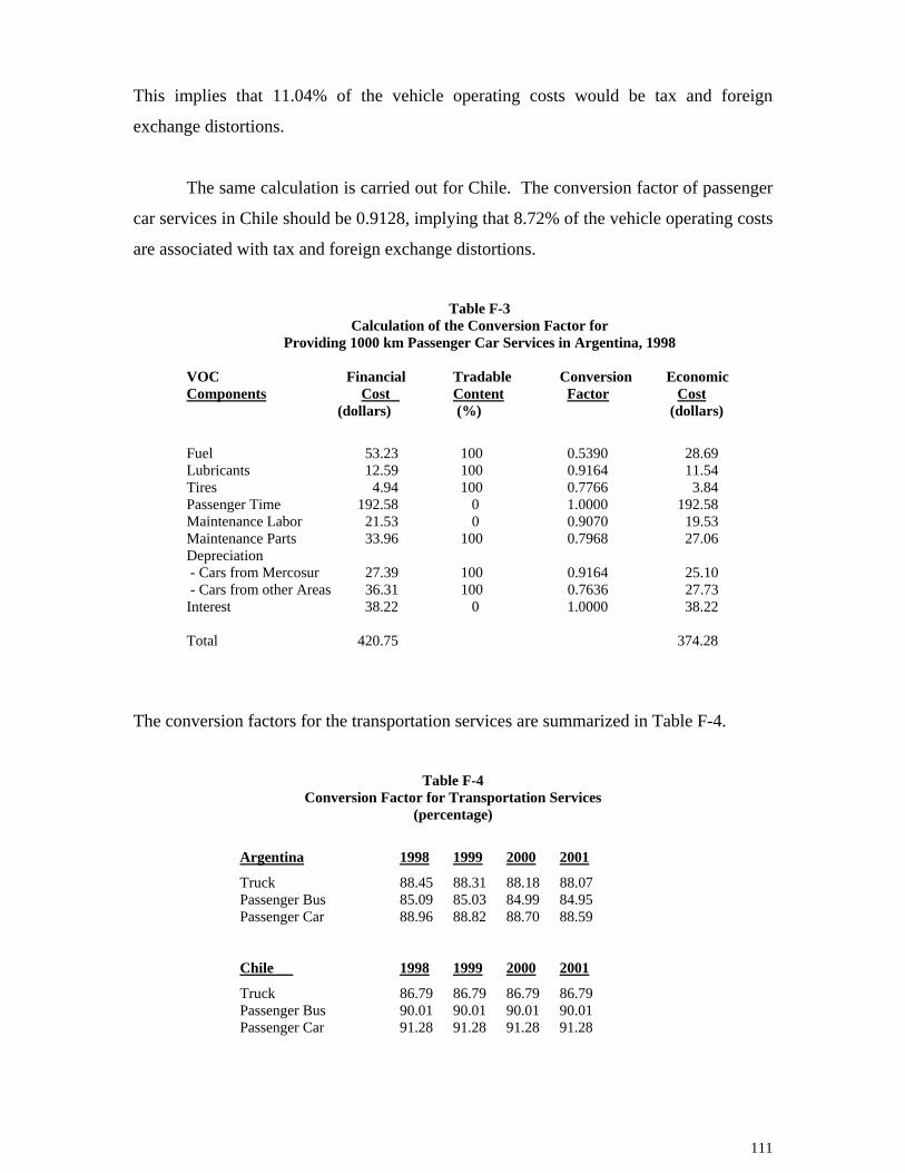
This implies that 11.04% of the vehicle operating costs would be tax and foreign
exchange distortions.
The same calculation is carried out for Chile. The conversion factor of passenger
car services in Chile should be 0.9128, implying that 8.72% of the vehicle operating costs
are associated with tax and foreign exchange distortions.
Table F-3
Calculation of the Conversion Factor for Providing 1000 km Passenger Car Services in Argentina, 1998
VOC Financial Tradable Conversion Economic Components Cost Content Factor Cost (dollars) (%) (dollars)
Fuel 53.23 100 0.5390 28.69 Lubricants 12.59 100 0.9164 11.54 Tires 4.94 100 0.7766 3.84 Passenger Time 192.58 0 1.0000 192.58 Maintenance Labor 21.53 0 0.9070 19.53 Maintenance Parts 33.96 100 0.7968 27.06 Depreciation - Cars from Mercosur 27.39 100 0.9164 25.10 - Cars from other Areas 36.31 100 0.7636 27.73 Interest 38.22 0 1.0000 38.22 Total 420.75 374.28
The conversion factors for the transportation services are summarized in Table F-4.
Table F-4
Conversion Factor for Transportation Services (percentage)
Argentina 1998 1999 2000 2001
Truck 88.45 88.31 88.18 88.07 Passenger Bus 85.09 85.03 84.99 84.95 Passenger Car 88.96 88.82 88.70 88.59
Chile 1998 1999 2000 2001
Truck 86.79 86.79 86.79 86.79 Passenger Bus 90.01 90.01 90.01 90.01 Passenger Car 91.28 91.28 91.28 91.28
111