AND REPRESENTATION THEORY arXiv:1512.08779v2 … · toroidal gl1 algebra, therefore our formulas can be interpreted as the characters of these representations. ... i . (1.3) The formula

arX

iv:1

512.

0877

9v4

[m

ath.

CO

] 1

0 Fe

b 20

18

PLANE PARTITIONS WITH A “PIT”: GENERATING FUNCTIONS

AND REPRESENTATION THEORY

M. BERSHTEIN, B. FEIGIN, G. MERZON

To Sasha Beilinson on the occasion of his birthday. At least one of the authors owes him a lot.

Abstract. We study plane partitions satisfying condition an+1,m+1 = 0 (this conditionis called “pit”) and asymptotic conditions along three coordinate axes. We find theformulas for generating function of such plane partitions.

Such plane partitions label the basis vectors in certain representations of quantumtoroidal gl1 algebra, therefore our formulas can be interpreted as the characters of theserepresentations. The resulting formulas resemble formulas for characters of tensor repre-sentations of Lie superalgebra glm|n. We discuss representation theoretic interpretationof our formulas using q-deformed W -algebra glm|n.

1. Introduction

In this paper we study certain problems of enumerative combinatorics of 3d Youngdiagrams, which are motivated by representation theory.

It is convenient to identify 3d Young diagrams with plane partitions, i.e., collection ofnonnegative integers ai,j such that ai,j ≥ ai+1,j , ai,j ≥ ai,j+1 and all but a finite numberof ai,j equals 0. Later we will also consider more general plane partitions.

Denote by |a| =∑ai,j, i.e., the number of boxes in the corresponding 3d Young

diagram. For any set A of plane partitions, define its generating function by∑

a∈A q|a|.

Such functions were extensively studied in enumerative combinatorics, for example, oneof MacMahon’s formulas has the form (see e.g. [36, 1.5 ex. 13(d)])

∑

{a|an+1,1=0}

q|a| = q−(n3)V (1, q, . . . , qn−1)

(q)n∞,

where V (x1, . . . , xn) =∏

i<j(xi−xj) is the Vandermonde product and (q)∞ =∏∞

k=1(1−qk).

The limit n→∞ gives well-known MacMahon formula for the generating function of allplane partitions:

∑a q

|a| =∏∞

k=1(1− qk)−k.

We study plane partitions satisfying the condition

an+1,m+1 = 0. (1.1)

We will call such condition “pit” in box (n + 1, m+ 1). Moreover we will consider planepartitions a = {aij} with an infinite number of non-zero ai,j and some of ai,j equal to ∞,satisfying the following asymptotic conditions

1. limj→∞

ai,j = νi, 2. limi→∞

ai,j = µj, 3. ai,j =∞ iff (i, j) ∈ λ, (1.2)

where ν, µ, λ are partitions (see Fig. 1).1

http://arxiv.org/abs/1512.08779v4

2 M. BERSHTEIN, B. FEIGIN, G. MERZON

m = n = 4ν = (2, 1, 1)

2

λ = (3, 2)3

µ = (3, 3, 2, 1)1

∞ ∞ ∞ 4 4 3 2 2 2 . . . 2

∞ ∞ 4 4 3 2 1 1 1 . . . 1

5 4 4 3 3 1 1 1 1 . . . 1

5 4 4 3 3 1 0 0 0 . . . 0

4 3 3 2

3 3 2 1

3 3 2 1

3 3 2 1

3 3 2 1

3 3 2 1

. . . . . . . . . . . .

3 3 2 1

Figure 1.

We denote by χn,mµ,ν,λ(q) the generating function of plane partitions which satisfy (1.1),

(1.2) (for the definition of |a| see (2.1)). It follows from these conditions that l(ν) ≤ n,l(µ) ≤ m, and λn+1 < m+ 1.

Note that asymptotic conditions (1.2) appear in the theory of topological vertex [38].The condition (1.1) also appeared in the strings theory, see [24]. Our motivation comesfrom representation theory, which we discuss below.

In some particular cases the formulas for functions χn,mµ,ν,λ(q) were known before. In

order to write down the answers we need some notation. By ρn we denote the partition(n − 1, n − 2, . . . , 1, 0), we omit the index n and write just ρ if the number of parts isclear from the context. For any partition of no greater then n parts λ = (λ1, λ2, . . . , λn)by qλ+ρ we denote (qλ1+n−1, . . . , qλn). By aλ+ρ(x1, . . . , xn) we denote the antisymmetricpolynomial:

aλ+ρ(x1, . . . , xn) = det(xλj+n−ji

)ni,j=1

. (1.3)

The formula for χn,mµ,ν,λ(q) is known in the case m = 0, i.e., when the “pit” is located

near the “wall”. Namely

χn,0∅,ν,λ(q) =

q∑n

i=1(λi+n−i)(νi+n−i)

(q)n∞aν+ρ(q

−λ−ρ), (1.4)

see, for example, [9, Theorem 4.6]. Clearly this is a generalization of the MacMahonformula given above. Another known case is where two asymptotic conditions vanishλ = µ = ∅, see [19], [20].

In our paper we find the formula for χn,mµ,ν,λ(q) in general case. Actually we prove three

formulas, which are algebraically equivalent but have different form and meaning. Theyare given in Theorems 1, 2, 3 below. Here we give the simplest (but already new) particular

PLANE PARTITIONS WITH A “PIT” 3

case of Theorem 2

χn,nµ,ν,∅(q) =

∑

A1>A2>...>An≥0

(−1)

n∑i=1

Ai

q

n∑i=1

(Ai+12 )aν+ρ(q

A)aµ+ρ(q−A)

(q)2n∞, (1.5)

Note that each summand is a product of two expressions on the right side of (1.4) (up tothe factor of the form (−1)...q...)

Since our three formulas are algebraically equivalent it is enough to prove any of them.We give two different combinatorial proofs, one for Theorem 1 and one for Theorem 3.These proofs are simpler than ones of particular cases given in [19], [20].

The first proof is based on a bijection between plane partitions and collections of noncrossing paths. The number of such collections is computed using Lindstrom–Gessel–Viennot lemma [30],[23]. Such proof gives a determinantal expression for χn,m

µ,ν,λ(q), seeTheorem 1.

In the second proof we interpret conditions (1.1),(1.2) as a definition of certain infinitedimensional polyhedron. We compute the generating function of integer points in thispolyhedron as a sum of contribution of vertices, using Brion theorem [6]. Such proof givesa “bosonic formula”1 for χn,m

µ,ν,λ(q), see Theorem 3.The conditions (1.1),(1.2) appeared in [13] in the context of representation theory of

quantum toroidal algebra U~q(gl1). Namely, plane partitions which satisfy these conditions

label a basis in MacMahon modules N n,mµ,ν,λ(v) over U~q(gl1). Therefore χn,m

µ,ν,λ(q) is the

character of the representation N n,mµ,ν,λ(v). It is natural to ask for representation theoretic

interpretation of our character formulas.We conjecture that there exist resolutions of N n,m

µ,ν,λ(v) such that their Euler charac-teristics coincide with our character formulas. In such cases we say that the resolutionis a materialization of the character formula. For example, the BGG resolution [5] is amaterialization of the Weyl character formula. Zelevinsky constructed complex which isa materialization of the Jacobi–Trudi formula for Schur polynomials [43].

Our formulas for functions χn,mµ,ν,λ(q) resemble the formulas for characters of tensor repre-

sentations of Lie superalgebra glm|n. This similarity can be explained by the fact that therepresentations N n,m

µ,ν,λ(v) are actually representations of certain q-deformed W -algebra,

which we call W~q(gln|m).Such W -algebras appear as follows. There is an easy (but not written in the literature)

fact that N n,mµ,ν,λ(v) is a subquotient of Fock representation of U~q(gl1). This Fock module

is a tensor product of n +m basic Fock modules, see the formula (5.17). On such Fock

modules the algebra U~q(gl1) acts through the its quotient which is called W -algebra. ThisW -algebra commutes with the certain intertwining operators, which are called screen-ing operators. The structure of the screening operators in our case suggests the nameW~q(gln|m).

There exists the conformal limit ~q → (1, 1, 1) of screening operators and we denote the

limit of the algebra W by W(gln|m). For m = 0 this algebra coincides with the algebra

W(gln) [32]. The algebras W(gln|1) conjecturally coincide with the “zero momentum”

1Usually a formula is called bosonic if it equals a linear combination of characters of algebra of poly-nomials. In our case bosonic formula is a combination of terms q∆/(q)n+m

∞ .


sector of W(2)n algebras introduced in [21]. We did not find reference for generic n,m.2

Note that our W -algebras differ from ones introduced in [27].Standard statement in the theory of vertex algebras is an equivalence of the abelian

categories of certain representations of vertex algebra and certain representations of quan-tum group. This is a statement similar to Drinfeld–Kohno or Kazhdan–Lusztig theorems.We conjecture that under this equivalence W(gln|m) is related to the product of quantumgroups Uqgln|m⊗Uq′gln⊗Uq′′glm for certain q, q′, q′′. And representations N n,m

µ,ν,λ(v) under

this equivalence go to the tensor products L(n|m)λ ⊗ L(n)

ν ⊗ L(m)µ , where L

(n)ν and L

(m)µ are

finite dimensional irreducible representations of Uq′gln and Uq′′glm, correspondingly, and

L(n|m)λ is a tensor representation of Uqgln|m (representations L

(n|m)λ , L

(n)ν , L

(m)µ also depend

on v but we omit this dependence for simplicity).

Plan of the paper. In Section 2 we give precise statements of our main results forχn,mµ,ν,λ(q) with necessary notation and comments. The remaining sections 3, 4, 5 are inde-

pendent of each other. Sections 3 and 4 are devoted to the combinatorial proofs based onLindstrom–Gessel–Viennot lemma and Brion theorem, correspondingly. Section 5 is de-voted to the algebraic discussion. First we give a definition of the appropriateW -algebrasin terms of screening operators. Conjectural materializations of our character formulasare discussed in subsection 5.5. Relation to quantum group Uqgln|m ⊗ Uq′gln ⊗ Uq′′glm isdiscussed in subsection 5.7.

Acknowledgments. We thank A. Babichenko, E. Gorsky, A. Kirillov, A. Litvinov,I. Makhlin, G. Mutafyan, G. Olshanski, Y. Pugai, A. Sergeev for interest to our workand discussions. We are grateful to anonymous referee for the careful reading and hugenumber of valuable comments.

This work has been funded by the Russian Academic Excellence Project 5-100. M. B. ac-knowledges the financial support of Simons-IUM fellowship, RFBR grant mol a ved 15-32-20974 and Young Russian Math Contest.

2. Main Results

2.1. Due to asymptotic conditions (1.2) ai,j ≥ νi and ai,j ≥ µj. In order to define thegrading |a| ∼

∑ai,j , we need to subtract these asymptotic values νi, µj .

We will use the following definition

|a| =∑

i−n≤j−m, (i,j)6∈λ

(ai,j − νi) +∑

i−n>j−m, (i,j)6∈λ

(ai,j − µj). (2.1)

Note that this definition of grading is not invariant under m,µ ↔ n, ν symmetry. Geo-metrically the definition (2.1) can be restated as follows. We draw a staircase line fromthe point (n,m) as on the picture below. This line divides the base of the plane partitiona into two parts. We subtract νi from cells in the upper part and µj from cells in the leftpart, see Fig. 2.

2Note added: After the first version of the paper appeared in the arXiv these W algebras (as wellas more generic, see Remark 5.1) were studied in the framework of conformal field theory [31] andsupersymmetric gauge theory [22].


−ν5 −ν5 −ν5 −ν5

−ν4 −ν4 −ν4 −ν4 −ν4

−ν3 −ν3 −ν3 −ν3 −ν3

−ν2 −ν2 −ν2 −ν2 −ν2

−ν1 −ν1 −ν1 −ν1

−µ1

−µ1

−µ1

−µ1

−µ2

−µ2

−µ2

−µ2

−µ2

−µ2

−µ3

−µ3

−µ3

−µ3

−µ3

−µ4

−µ4

−µ4

−µ4

Figure 2.

Let r = min{t|λn−t ≥ m − t}, 0 ≤ r ≤ min{n,m}. Geometrically r is the number ofhorizontal steps in the staircase line starting from the point (m,n). In the Fig. 2 we haver = 2. Note that this number r has an interpretation in terms of representation theory ofgl(m|n), namely, r is called the degree of atypicality (or simply atypicality) of the tensorrepresentation of gl(m|n) corresponding to λ (see, for example [37, page 9]).

In order to write down the formula for the generating function we parametrize λ by someanalogue of Frobenius coordinates. We introduce two partitions π, κ by πi = λi− (m− r)for i = 1, . . . , n − r and κj = λ′j − (n − r) for j = 1, . . . , m − r, where λ′ denotes thetranspose of the partition λ. We denote components of partitions ν, µ, π, κ shifted by ρ bythe corresponding capital Latin letters: Ni = νi+n−i,Mj = µj+m−j, Pi = πi+(n−r)−i,Qj = κj + (m− r)− j.

2.2. In the simplest case n = 1, m = 0 for any asymptotic conditions λ, ν the generatingfunction of partitions χ1,0

∅,ν,λ(q) equals 1/(q)∞ (and similarly for n = 0, m = 1 case).Now consider the n = m = 1 case. If λ 6= ∅ then the plane partitions decompose into

two partitions so the generating function equals 1/(q)2∞. In the case λ = ∅, there is aclear bijection between plane partitions and V -partitions [41] i.e. the N-arrays of integernumbers: (

a0a1 a2 a2 . . .b1 b2 b2 . . .

),

such that a0 ≥ a1 ≥ a2 ≥ . . ., a0 ≥ b1 ≥ b2 ≥ . . ., limi→∞ ai = ν1, limi→∞ bi = µ1. Theweight of the V -partition is defined as

N =∑

i≥0

(ai − ν1) +∑

i≥1

(bi − µ1).


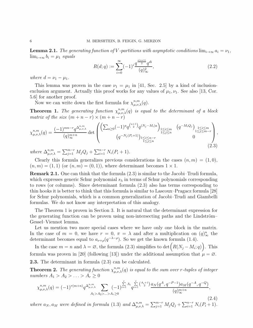
Lemma 2.1. The generating function of V -partitions with asymptotic conditions limi→∞ ai = ν1,limi→∞ bi = µ1 equals

R(d; q) :=∞∑

i=0

(−1)iq

i(i+1)2 qdi

(q)2∞, (2.2)

where d = ν1 − µ1.

This lemma was proven in the case ν1 = µ1 in [41, Sec. 2.5] by a kind of inclusion-exclusion argument. Actually this proof works for any values of µ1, ν1. See also [13, Cor.5.6] for another proof.

Now we can write down the first formula for χn,mµ,ν,λ(q).

Theorem 1. The generating function χn,mµ,ν,λ(q) is equal to the determinant of a block

matrix of the size (m+ n− r)× (m+ n− r)

χn,mµ,ν,λ(q) =

(−1)mn−rq∆n,mµ,ν,λ

(q)m+n∞

det

(∑a≥0(−1)

aq(a+12 )q(Nj−Mi)a

)1≤i≤m1≤j≤n

(q−MiQj

)1≤i≤m

1≤j≤m−r(q−Nj(Pi+1)

)1≤i≤n−r1≤j≤n

0

,

(2.3)where ∆n,m

µ,ν,λ =∑m−r

j=1 MjQj +∑n−r

i=1 Ni(Pi + 1).

Clearly this formula generalizes previous considerations in the cases (n,m) = (1, 0),(n,m) = (1, 1) (or (n,m) = (0, 1)), where determinant becomes 1× 1.

Remark 2.1. One can think that the formula (2.3) is similar to the Jacobi–Trudi formula,which expresses generic Schur polynomial sλ in terms of Schur polynomials correspondingto rows (or columns). Since determinant formula (2.3) also has terms corresponding tothin hooks it is better to think that this formula is similar to Lascoux–Pragacz formula [28]for Schur polynomials, which is a common generalization of Jacobi–Trudi and Giambelliformulas. We do not know any interpretation of this analogy.

The Theorem 1 is proven in Section 3. It is natural that the determinant expression forthe generating function can be proven using non-intersecting paths and the Lindstrom–Gessel–Viennot lemma.

Let us mention two more special cases where we have only one block in the matrix.In the case of m = 0, we have r = 0, π = λ and after a multiplication on (q)n∞ thedeterminant becomes equal to aν+ρ(q

−λ−ρ). So we get the known formula (1.4).

In the case m = n and λ = ∅, the formula (2.3) simplifies to det(R(Nj−Mi; q)

). This

formula was proven in [20] (following [13]) under the additional assumption that µ = ∅.

2.3. The determinant in formula (2.3) can be calculated.

Theorem 2. The generating function χn,mµ,ν,λ(q) is equal to the sum over r-tuples of integer

numbers A1 > A2 > . . . > Ar ≥ 0

χn,mµ,ν,λ(q) = (−1)r(m+n)q∆

n,mµ,ν,λ

∑

A1>A2>...>Ar≥0

(−1)

r∑i=1

Ai

q

r∑i=1

(Ai+12 )aN(q

A, q−P−1)aM(q−A, q−Q)

(q)m+n∞

,

(2.4)where aN , aM were defined in formula (1.3) and ∆n,m

µ,ν,λ =∑m−r

j=1 MjQj +∑n−r

i=1 Ni(Pi +1).


-1 0 1

Figure 3.

Lemma 2.2. The r.h.s. of (2.3) and (2.4) are equal.

Our proof of this lemma is based on a direct calculation, which we present in Subsec-tion 3.4.

There are two special cases in which the right side takes a simpler form. These twospecial cases of the theorem were known.

First, if m = 0 then the formula (2.4) reduces to (1.4). More generally if r = 0, thenbase of the plane partition decomposes into two connected components and the formula

(2.4) becomes a product q∆n,mµ,ν,λaN (q

−P−1)aM(q−Q)/(q)m+n∞ .

In the second case we take λ = µ = ν = ∅. Then the functions aN and aM reduce toVandermonde products and we can write (we assume that n ≥ m)

χn,m∅,∅,∅(q)

=q∆

n,m∅,∅,∅

(q)m+n∞

∑

A1>A2>...>Am≥0

(−1)

m∑i=1

(Ai−i+1)q

m∑i=1

(Ai+12 )

V (qm−n, . . . , q−1, qAm, . . . , qA1)V (q−A1 , . . . , q−Am)

=1

(q)m+n∞

∑

α1≥α2≥...≥αm≥0

(−1)

m∑i=1

αi

q

m∑i=1

12αi(αi+(2i−1)) ∏

1≤i<j≤m

(1−qαi−αj−i+j)∏

1≤i<j≤n

(1−qαi−αj−i+j).

(2.5)

Here we set αj = 0 for j > m. This formula coincides with the [13, Conjecture 5.10]proved in [19, Theorem 1.2] by a completely different method.

2.4. The sum in formula (2.4) contains zero terms if one of Ai equals to one of Qj . Wewant to exclude such terms. The following lemma is standard.

Lemma 2.3. For any partition λ we have

Z = {λ′j − j − (n−m)|j ∈ N}⊔{i− λi − (n−m)− 1|i ∈ N}.

Sketch of the proof. The proof is based on the following construction. Rotate Young dia-gram corresponding to λ by 135◦ and take a projection on OX . On the Fig 3 we give anexample for λ = (4, 4, 4, 3, 3, 1).


It is easy to see that x-coordinates of white balls are i−λi−12and coordinates of black

ones are λ′j−j+12. Therefore Z+ 1

2= {λ′j−j+

12}⊔{i−λi−

12}. Shifting by −(n−m)− 1

2we get the Lemma. �

Recall that

Qj = κj − j +m− r = λ′j − j − (n−m) for 1 ≤ j ≤ m− r.

Note that λ′j − j − (n − m) ≥ 0 if and only if 1 ≤ j ≤ m − r. Since A1, . . . , Ar ≥ 0and Ai 6= Qj then it follows from the Lemma 2.3 that {Ai} should be a subset in the set{i− λi − (n−m)− 1|i ∈ N}. Note that i− λi − (n−m)− 1 ≥ 0 if and only if i > n− r.Therefore, the non-zero terms correspond to subsets {Ar, . . . , A1} ⊂ {−Li|i > n − r},where Li = λi − i + n − m + 1. Rewriting the determinants in (2.4) as sums overpermutations we get the following result.

Theorem 3. The generating function χn,mµ,ν,λ(q) is equal to the sum

χn,mµ,ν,λ(q) = (−1)r(m+n)

∑

(σ,τ,A)∈Θ

(−1)|σ|+|τ |+

r∑i=1

Ai q∆σ,τ,A(µ,ν,λ)

(q)n+m∞

, (2.6)

where

(σ, τ, A) ∈ Θ⇔ σ ∈ Sn, τ ∈ Sm, Ar−i+1 = −Lsi , for sr > · · · > s1 > n− r,

and

∆σ,τ,A(µ, ν, λ) =r∑

i=1

Ai

(Ai + 1

2+Nσ(i) −Mτ(i)

)

−n∑

i=r+1

(Pi−r + 1)(Nσ(i) −Ni−r)−m∑

i=r+1

Qi−r(Mτ(i) −Mi−r).

This theorem will be proven in Section 4. In this proof we consider inequalitiesai,j ≥ ai+1,j , ai,j ≥ ai,j+1 and conditions (1.2) as a definition of a polyhedron (infinitedimensional) and the generating function χn,m

µ,ν,λ(q) as a sum over integer points in thepolyhedron. This sum is calculated using Brion theorem [6]. Each term in (2.6) corre-sponds to a vertex contribution in Brion theorem.

3. Lattice paths

3.1. Let G be an oriented graph with the set of vertices V and the set of edges E. Toany edge e ∈ E we assign a weight w(e). For any path p = (e1, e2, . . . , en) we define theweight as a product of the edge weights w(p) =

∏w(ei).

For any two vertices s, t we denote P (s→ t) =∑

pw(p), where the summation goes

over all paths from s to t. Below we will assume that P (s→ t) is well-defined. Usuallythis follows from the condition that number of paths from s to t is finite (for example in[1] this follows from the conditions that G is finite and has no oriented cycles). In ourcase the weight of the edge w(e) ∈ {qZ≥0}, where q is a formal variable, and we assumethat for any fixed H ∈ Z≥0 number of paths from s to t of the weight qH is finite. ThenP (s→ t) is well-defined as a formal series in q, P (s→ t) ∈ C[[q]].


For any sets of n source vertices S = {s1, . . . , sn} and n target vertices T = {t1, . . . , tn}we denote P (S→T ) =

∑p1,...,pn

w(p1) · . . . ·w(pn), where the summation goes over all sets

of paths such that pi goes from si to ti. Clearly P (S→T ) = P (s1→ t1) · . . . · P (sn→ tn).By Pnc(S → T ) we denote the sum

∑p1,...,pn

w(p1) · . . . · w(pn) where set of paths isassumed to be without crossings. The Lindstrom-Gessel-Viennot lemma provides an ef-ficient way to find Pnc(S→T ). Standard references for this lemma are [30], [23], for theclear introduction see [1].

Lemma (Lindstrom-Gessel-Viennot). For an oriented graph G as above and any sets ofsources and targets S = {s1, . . . , sn}, T = {t1, . . . , tn} we have

∑

σ∈Sn

(−1)|σ|Pnc(S→σ(T )) = det(P (si→ tj)

)ni,j=1

In most examples (and in all examples in this paper) Pnc(S→σ(T )) 6= 0 for only onepermutation σ. In this case

Pnc(S→σ(T )) = (−1)|σ| det(P (si→ tj)

)ni,j=1

.

3.2. In this paper we use graph G with vertices (a+ 12, b), where a, b ∈ Z, b ≥ 0. There are

two types of edges namely the horizontal ones (a+12, b)→ (a+3

2, b) (→ denotes orientation)

and vertical ones (a + 12, b) → (a + 1

2, b+ 1) for a < 0 and (a + 1

2, b) ← (a + 1

2, b+ 1) for

a ≥ 0. The weight of a vertical edge is 1, the weight of a horizontal edge on the line y = bis qb.

Note that the number of paths from s = (12, b) to t = (1

2+ a, 0), a, b ≥ 0 is equal to

the binomial coefficient(a+bb

). The number of paths counted with weights is equal to the

q-binomial coefficient P (s→ t) =[a+bb

]q.

We will use “infinitely remote” source and target vertices, see an example in Fig. 4.We say that a path starts at the point (−∞, b) if the path contains all sufficiently leftedges on the horizontal line y = b. Similarly we define paths which start at the point(a,+∞) or go to the point (+∞, b) or (a,+∞). For example, the paths from the points = (−∞, 0) to t = (−1

2,+∞) are in one to one correspondence with Young diagrams.

And in this case P (s→ t) is equal to the generating function of Young diagrams 1/(q)∞.For the “infinitely remote” source and target vertices we need to define the weight of the

path. The problem happens for the vertices (−∞, b) since their paths contain infinitelymany horizontal edges on the line y = b and therefore the weights of these paths are notdefined. We divide by qb the weight of each horizontal edge (of such paths) over the point(i, 0), i < 0. Clearly there is no more than one such edge, if there is none we just dividethe weight of the path by qb. Informally speaking, we assign the weight q−b(∞/2−1/2) tothe vertex (−∞, b). For example, for s = (−∞, b), t = (−a − 1

2,+∞), a, b ≥ 0 we have

P (s→ t) = q−ab/(q)∞.For the (+∞, b) we divide by qb the weight of each horizontal edge (of path to the

(+∞, b)) over the point (i, 0), i ≥ 0. Informally speaking we assign the weight q−b(∞/2+1/2)

to the vertex (+∞, b). For example, for s = (a + 12,+∞), t = (+∞, b), a, b ≥ 0 we have

P (s→ t) = q−(a+1)b/(q)∞.


Now we prove the formula (1.4) for the number of plane partitions with n rows andasymptotic conditions.

Proposition 3.1. The generating function of plane partitions {ai,j}, such that 1 ≤ i ≤ n,j ∈ N, ai,j =∞ iff (i, j) ∈ λ, limj→∞ aij = νi has the form

χn,0∅,ν,λ(q) =

q∑n

i=1(λi+n−i)(νi+n−i)

(q)n∞aν+ρ(q

−λ−ρ).

Proof. There is a natural bijection between such plane partitions and collections of non-intersecting paths from S = {s1, . . . , sn}, si = (λi + n − i + 1

2,+∞) to T = {t1, . . . , tn},

ti = (+∞, νi + n − i). The first row of the plane partition encodes the path from s1 tot1, the second row of the plane partition encodes the path from s2 to t2 and so on. Thecoordinates of the sources and targets are specified in such a way that plane partitioncondition ai,j ≥ ai+1,j is equivalent to the non-intersection of paths.

In the Fig. 4 we give an example, where n = 3, λ = (2, 1, 1), ν = (3, 1, 1).

∞∞ 3 3 3 3 3 3 3 . . . 3∞ 3 3 2 1 1 1 1 1 . . . 1∞ 3 3 1 1 1 1 1 1 . . . 1

←→

s3 s2 s1

t3

t2

t1

Figure 4.

As was noted before we have P (si→ tj) = q−(λi+n−i+1)(νj+n−j)/(q)∞. Therefore usingthe Lindstrom-Gessel-Viennot lemma we get

P (S→T ) = det

(q−(λi+n−i+1)(νj+n−j)

(q)∞

).

Note that the function P (S→T ) differs from χn,0∅,ν,λ(q) by a certain power of q since our

grading on paths differs slightly from the definition (2.1). In particular, χn,0∅,ν,λ(q) has the

leading term 1, but P (S→ T ) has the leading term q−∑

i(λi+n−i+1)(νi+n−i). MultiplyingP (S→T ) by q

∑i(λi+n−i+1)(νi+n−i) we get Proposition 3.1. �

3.3. We have not discussed one type of paths between “infinitely remote” vertices. Namelylet s = (−∞, b), t = (+∞, a). Then the paths from s to t are in one-to-one correspondencewith V -partitions with asymptotic conditions limi→∞ ai = a, limi→∞ bi = b, see Fig. 5.

Recall that the generating function of V -partitions was given in Lemma 2.1 and equalsR(a− b; q). Now we are ready to prove Theorem 1.


(5

4 4 2 2 . . .3 3 1 1 . . .

)←→

s t

Figure 5.

Proof of Theorem 1. First, we use a one-to-one correspondence between plane partitionssatisfying (1.2),(1.1) and certain lattice paths. We decompose the base of plane partitioninto r infinite hooks, m− r infinite columns and n− r infinite rows.

We set the sources and targets to be the points

si =

(−∞,Mi) for 1 ≤i ≤ m,

(Pi−m +1

2,+∞) for m+ 1 ≤i ≤ m+ n− r

,

tj =

(+∞, Nj) for 1 ≤j ≤ n,

(−Qj−n −1

2,+∞) for n + 1 ≤j ≤ m+ n− r

.

We illustrate the correspondence in the Fig. 6, where we have n = 3, m = 2,λ = (2, 1, 1), ν = (3, 1, 1), µ = (2, 0). By previous definitions r = 1, π = (1, 0), κ = (1),N1 = 5, N2 = 2, N3 = 1, M1 = 3, M2 = 0, P1 = 2, P2 = 0, Q1 = 1.

∞∞ 3 3 3 3 3 3 3 . . . 3∞ 3 3 2 1 1 1 1 1 . . . 1∞ 3 3 1 1 1 1 1 1 . . . 1

4 2

3 1

2 0

2 0. . . . . .

2 0

←→

s2

s1

s4 s3t4

t3

t2

t1

Figure 6.

Due to our order of si and tj non-intersecting paths correspond to the permutation(s1 s2 . . . sm−r sm−r+1 . . . sm sm+1 . . . sm+n−r−1 sm+n−r

tn+1 tn+2 . . . tm+n−r tn−r+1 . . . tn t1 . . . tn−r−1 tn−r

)


We denote this permutation of indexes 1, . . . , m+ n− r by σm,n,r. So we proved that

χn,mµ,ν,λ(q) = q...P (S→σm,n,r(T )).

We compute the value P (S→ σm,n,r(T )) from the Lindstrom-Gessel-Viennot lemma.The number of inversions in the permutation σm,n,r is equal to mn − r2. It remains toevaulate P (si→ tj), which have been actually found above

P (si→ tj) =

R(Nj −Mi; q) for 1 ≤ i ≤ m, 1 ≤ j ≤ n,

q−MiQj−n/(q)∞ for 1 ≤ i ≤ m, n+ 1 ≤ j ≤ m+ n− r

q−Nj(Pi−m+1)/(q)∞ for m+ 1 ≤i ≤ m+ n− r, 1 ≤ j ≤ n

0 for m+ 1 ≤i ≤ m+ n− r, n+ 1 ≤ j ≤ m+ n− r

.

Combining all together we obtain Theorem 1. As above, the additional factor q∑m−r

j=1 MjQj+∑n−r

i=1 Ni(Pi+1)

comes from the difference between definition of grading in terms of paths and (2.1). �

3.4. In this Subsection we prove Lemma 2.2.

Proof. We want to calculate the determinant of the matrix

M =

(∑a≥0(−1)


)1≤i≤m1≤j≤n

(q−MiQj

)1≤i≤m


)1≤i≤n−r1≤j≤n

0

.

Denote

M =

(∑a≥0(−1)


)1≤i≤m1≤j≤n

((−1)Qjq(

Qj+1

2 )q−MiQj

)1≤i≤m


)1≤i≤n−r1≤j≤n

0

.

Clearly, we have detM = Cdet M, where C = (−1)∑

Qjq−∑(Qj+1

2 ). We decompose the

matrix M as a product of two (infinite) matrices

M =

0((−1)aq(

a+12 )−aMi

)1≤i≤m,a≥0

(δ−a−1,Pi)1≤i≤n−r,

a<00

((qaNj

)a∈Z,

1≤j≤n

((−1)Qjδa,Qj

)a∈Z,

1≤j≤m−r

),

Now we apply the Cauchy–Binet formula, the numbers of columns in the minor fromthe first factor (the numbers of rows in the minor from the second factor) we denote by−P1 − 1, . . . ,−Pn−r − 1, A1, . . . , Ar, Q1, . . . , Qm−r, and get

detM = (−1)(m−r)(n−r)∑

A1>A2>...>Ar≥0

(−1)

r∑i=1

Ai

q

r∑i=1

(Ai+12 )

aN(qA, q−P−1)aM(q−A, q−Q)

In this sum we a-priori have extra condition Ai 6= Qj but we ignore it since the corre-sponding terms vanish.

Therefore we proved that the right sides of (2.3) and (2.4) are equal. �


4. Integer Points in Polyhedra

4.1. In this section we give a combinatorial proof of Theorem 3. The proof is based onBrion’s theorem which we briefly recall. Standard references for this theorem are [6], [33],[34], [29], for a clear introduction see, for example, [3].

Let P ⊂ RN be a convex polyhedron, i.e., an intersection of a finite number of half-spaces. Note that P can be unbounded. For simplicity we assume below that vertices ofP have integer coordinates and edges have rational directions.

For a point p = (p1, . . . , pN) ∈ ZN by tp we denote tp11 · · · tpNN , where t1, . . . , tN are

formal variables. Define the characteristic function of P by the formula

S(P ) =∑

p∈P∩Zn

tp.

In this definition S(P ) is a formal series, S(P ) ∈ Z[[t±11 , . . . , t±1

N ]]. It can be proven thatthere exist two Laurent polynomials f, g ∈ Z[t±1

1 , . . . , t±1N ] such that fS(P ) = g (see e.g.

[2, Theorem 13.8]). We denote S(P ) = g/f ∈ Q(t1, . . . , tn). Clearly S(P ) does not dependon the particular choice of f, g ∈ Z[t±1

1 , . . . , t±1N ]

For any vertex v ∈ P , we denote by Kv its cone, i.e., the intersection of half-spacescorresponding to the facets (maximal proper faces) of P containing v.

Theorem (Brion). For any convex polyhedron P with integer vertices and rational direc-tions of edges we have

S(P ) =∑

v

S(Kv).

Plane partitions satisfying (1.1) and (1.2) are integer points of the polyhedron P n,mµ,ν,λ

in the space with coordinates ti,j (i, j) ∈ N2 \ λ. The polyhedron P n,mµ,ν,λ is defined by the

inequalities

P n,mµ,ν,λ :

ti,j ≥ ti,j+1 ti,j ≥ νi ≥ 0

ti,j ≥ ti+1,j ti,j ≥ µj ≥ 0

tn+1,m+1 = 0

, (4.1)

Therefore the functions χn,mµ,ν,λ(q) can be computed using Brion theorem.

Two remarks are in order. First, we stated Brion theorem for finite dimensional poly-hedra, but P n,m

µ,ν,λ is infinite dimensional. Therefore we start from the finitization of P n,mµ,ν,λ,

i.e., for H,H ′ ∈ N we consider the polyhedron Pn,m,(H,H′)µ,ν,λ defined as

Pn,m,(H,H′)µ,ν,λ :

ti,j ≥ ti,j+1 ti,H = νi ≥ 0

ti,j ≥ ti+1,j tH′,j = µj ≥ 0

tn+1,m+1 = 0

, (i, j) ∈ {1, . . . , H ′} × {1, . . . , H} \ λ.

(4.2)We compute S(P n,m,(H,H′)) and then take the limit H,H ′ →∞.

Second, we need a specialization of the function S(P ) in which ti,j → q. We denoteby Sq(P ) ∈ Q(q) the function obtained by composition of S and this specialization. The

limit limH,H′→∞ q−∆(H,H′)Sq(P

n,m,(H,H′)µ,ν,λ ) coincides with χn,m

µ,ν,λ(q). Here the numbers ∆(H,H′)

emerge due to different definitions of grading, see below.


It will be convenient to start from a specialization ti,j → xj−i+1/xj−i. We denote bySx(P ) ∈ Q({xi}) composition of S and this specialization. Then we can set xi → qi andget Sq(P ).

4.2. We explain main ideas in the case m = 0. As the result we get a new proof of (1.4).We will work under an additional assumption of strict inequalities

ν1 > . . . > νn,

in the Section 4.4 we briefly explain (following [35]) how to remove this assumption.

We start from a description of vertices of the polyhedron Pn,0,(H,H′)∅,ν,λ . Since tn+1,1 = 0

one can think that indices (i, j) of coordinates ti,j satisfy 1 ≤ i ≤ n, 1 ≤ j ≤ H , (i, j) 6∈ λ,i.e., (i, j) lies in a skew Young diagram that we will denote (Hn) − λ. Any face of ourpolyhedron is defined by (4.2) where some of the inequalities become equalities. For anyface we construct a graph Γ with vertices (i, j) satisfying conditions above. Two vertices(i, j) and (i′, j′) are connected by an edge iff ti,j = ti′,j′ for all points of the face and boxes(i, j) and (i′, j′) have a common side.

There exist at least n connected components in Γ since ti,H = νi and νi > νj for i > j.Vertices of our polyhedron are faces of maximal codimension, i.e., corresponding to graphshaving exactly n connected components. See an example in Fig. 7.

ν1

ν2

ν3

ν4

Figure 7.

Denote by Γv the graph corresponding to the vertex v. Denote by Ks connected com-ponents of Γv. Each Ks is a skew Young diagram. Denote by Ks,v projection of the coneKv on the subspace with coordinates ti,j for (i, j) ∈ Ks. The inequalities defining the coneKv come from the equalities defining the vertex v and therefore do not include ti,j fromdifferent connected components. Therefore the cone Kv is a product of its projectionsKs,v, and we have S(Kv) =

∏S(Ks,v).

Situation simplifies since for many vertices Sq(Kv) vanishes due to the following result.

Proposition 4.1 ([35, Theorem 2.1]). If the connected component Ks has cycles, thenSx(Ks,v) is equal to 0.

In particular, from this Proposition and calculation in acyclic case below follows that

specializations Sq(Kv) (and therefore Sq(Pn,0,(H,H′)∅,ν,λ )) are well-defined. Similar argument

works for generic Sq(Pn,m,(H,H′)µ,ν,λ ), see the section 4.3

Therefore by Brion theorem we have

Sq(Pn,0,(H,H′)∅,ν,λ ) =

∑

v

Sq(Kv), (4.3)


where the summation goes over the vertices v such that corresponding graphs Γv areacyclic.

Recall that a skew Young diagram α − β is called a ribbon if it is connected and

contains no 2 × 2 block of squares. Due to Proposition 4.1, vertices of Pn,0,(H,H′)∅,ν,λ with

nonzero contribution correspond to decompositions of the skew diagram (Hn)− λ into nribbons such that boxes (i, H) belong to different ribbons.3

In order to discuss ribbons it is convenient to use also another combinatorial description.For any partition λ we assign sequence of numbers λi−i. This map is the bijection betweenpartitions and sequences {ai|i ∈ Z>0} such that ai > ai+1 and ai = −i for i >> 0. Wewill say that there are particles in the points λi− i and holes on the other integer points.For the illustration see Fig. 3, black balls are particles, white balls are holes (up to totalshift by 1

2).

The following lemma is standard

Lemma 4.1. Skew partition α−β is a ribbon if and only if there exist j, k ∈ N such thatthe set {αi − i} is obtained from the set {βi − i} by replacement of βj − j by βj − j + k.

We will call such replacement of βj − j by βj − j + k as jump of the particle βj − j.Therefore, in a more informal language the lemma means that a jump of one particle tothe right corresponds to the addition of a ribbon to partition. The decomposition of skewpartition into n ribbons corresponds to the sequence of n jumps of particles.

Assume that H > λ1+n−1. Then the sets of particles for partitions (Hn) and λ differin the first n numbers. Therefore to any decomposition of the skew diagram (Hn) − λinto n ribbons we assign a permutation σ ∈ Sn such that corresponding jumps are fromλi− i to H−σ(i). Since the boxes (i, H) belong to different ribbons the order of jumps isunique: first jump goes to H − 1, second to H − 2 and so forth. On the other side to anypermutation we assign the sequence of jumps due to ”only if” part of the Lemma 4.1 geta decomposition of skew diagram (Hn)− λ into n ribbons such that boxes (i, H) belongto different ribbons.

So we get a one-to-one correspondence between acyclic graphs Γv and permutations.

For example the graph Γv in the Fig. 8 corresponds to the permutation

(1 2 3 4

1 4 3 2

).

y − x = λ1 − 0

y − x = λ2 − 1

y − x = λ3 − 2

y − x = λ4 − 3

ν1

ν2

ν3

ν4

Figure 8.

We denote by vσ the acyclic vertex corresponding to σ ∈ Sn.

3One can compare this to Murnaghan–Nakayama rule.


Lemma 4.2. For the vertex vσ of the polyhedron Pn,0,(H,H′)∅,ν,λ we have

Sq(Kvσ) = (−1)|σ|q∆σ,(H)(λ,ν)/

n∏

i=1

(q)H−σ(i)−λi+i−1, (4.4)

where (q)k =∏k

s=1(1− qs) and

∆σ,(H)(λ, ν) =

n∑

i=1

(Hνi − iλi − iνi + i2)−n∑

i=1

(λi − i)(νσ(i) − σ(i)).

The proof is similar to the one in [35, Prop. 2.4].

Proof. Let Ki be the ribbon which corresponds to particle jump from λi− i by H − σ(i).The set {Ki} is a set of all connected components of the graph Γvσ . First, we computethe contribution of the corresponding cone S(Ki,vσ).

Denote by h the number of boxes in the ribbon Ki, clearly h = H − σ(i)− λi + i. Wenumber these boxes by 1, . . . , h from the bottom-left corner to the top-right corner. Inorder to simplify notation we denote the corresponding coordinates tk,j by t1, . . . , th. Inthe vertex vi of the cone Ki,vσ all these coordinates equal νσ(i), therefore Sq(t

vi) = qνσ(i)h.The cone Ki,vσ is simple. Its edges are generated by the vectors e1, . . . , eh−1, where the

vector es equals ±(1, . . . , 1, 0, . . . , 0), with s nonzero coordinates. The sign “±” is equalto “+” if the box s + 1 is a right neighbor of the box s and is equal to “−” if the boxs+ 1 is an upper neighbor of the box s. See an example in Fig. 9

e1

−1

e2

+1

+1

e3

+1

+1 +1

e4

−1

−1 −1 −1

e5

−1

−1 −1 −1

−1

e6

+1

+1 +1 +1

+1

+1

Figure 9.

Therefore Sq(Ki,vσ) = qνσ(i)h/∏h−1

s=1 (1− q±s), where the signs “±” were specified above.

Now we want to express this product in more explicit terms.

Lemma 4.3. The box s+ 1 is an upper neighbor of the box s if and only if there exists jsuch that i > j, σ(i) < σ(j) and s = λj − j − λi + i

In terms of particles this lemma means that particle λi − i in its jump overtakes theparticle λj − j and s in lemma corresponds to overtaking place.

Proof of the Lemma. We draw lines given by equations y = x + c, where c ∈ Z. Suchlines go through centers of boxes in our skew diagram (Hn) − λ. Such a line intersectsthe ribbon Ki in one box if λi − i+ 1 ≤ c ≤ H − σ(i) and does not intersect otherwise.

If the box s + 1 is an upper neighbor of the box s, then the right neighbor of the boxs belongs to another ribbon. Denote this ribbon by Ki′ and let this box (right neighborof the box s) has the number s′ + 1 in the ribbon Ki′.


If s′ > 0 then there is a previous box in the ribbon Ki′. This box has number s′ in Ki′

and should be the lower neighbor of the box s′ +1. And again, the right neighbor shouldbelong to another ribbon, denote this ribbon by Ki′′ and let this box has the numbers′′ + 1. This process lasts until we come to the first box of a certain ribbon, denote thisribbon by Kj .

Note that centers of boxes s+ 1 of Ki, s′ + 1 of Ki′, s

′′ + 1 of Ki′′. . . belong to the linegiven by equations y = x + c. Since this line goes through the center of the first box onKj we have c = λj − j + 1. Therefore s = λj − j − λi + i. In such case σ(i) < σ(j) sinceKj is below Ki, but i > j since s > 0.

See the Figure 8 for the demonstration of this effect.Conversely, for any j such that j > i and σ(j) < σ(i) consider the first box of Kj . The

line y = x+ c for c = λj − j + 1 goes through the center of this box and should intersectthe ribbon Ki. Let the box of intersection has number s+ 1 in Ki. Since σ(i) < σ(j) theribbon Ki is higher then the ribbon Kj and the box s + 1 in Ki is higher then the firstbox in the ribbon Kj . The box s + 1 in Ki cannot be the first box of the ribbon sinceλi− i 6= λj − j. And it is easy to prove similarly to the previous paragraphs that the boxnumber s is low neighbor of the box s+ 1. �

Rewriting factors 1/(1− q−s) as −qs/(1− qs) and using formula for h we have

Sq(Ki,vσ) = (−1)|{j:j<i,σ(j)>σ(i)}|qνσ(i)(H−σ(i)−λi+i)+

∑

j<i,σ(j)>σ(i)

(λj−j−λi+i)/

H−σ(i)−λi+i−1∏

s=1

(1− qs)

Now we can find Sq(Kvσ) =∏n

i=1 Sq(Ki,vσ). Using algebraic identities

∑

j<i,σ(j)>σ(i)

(λj − j − λi + i

)=

n∑

i=1

(λi − i)(σ(i)− i) (4.5)

andn∑

i=1

νσ(i)(H − σ(i)− λi + i) +

n∑

i=1

(λi − i)(σ(i)− i) = ∆σ,(H)(λ, ν)

we get (4.4). �

Now we can find Sq(Pn,0,(H,H′)∅,ν,λ ) using specialization of Brion theorem (4.3)

Sq(Pn,0,(H,H′)∅,ν,λ ) =

∑

σ∈Sn

(−1)|σ|q∆σ,(H)(λ,ν)/

n∏

i=1

(q)H−σ(i)−λi+i−1.

Here we count integer points in Pn,0,(H,H′)∅,ν,λ with the weight q

∑ti,j , which differs from the

weight defined in formula (2.1) by q∆(H)

, where ∆(H) =∑n

i=1 νi(H − λi). Using identity

∆σ,(H)(λ, ν)−∆(H) =

n∑

i=1

(νi + n− i)(λi + n− i)−n∑

i=1

(λi + n− i)(νσ(i) + n− σ(i))


we see that limit limH→∞ q−∆(H)Sq(P

n,0,(H,H′)∅,ν,λ ) coincides with the right side of (1.4).

4.3. In this subsection we prove Theorem 3 under the assumption

ν1 > . . . > νn > µ1 > . . . > µm. (4.6)

The Theorem 3 is valid without this assumption and later, in subsection 4.4, we explainthis.

Proof. As before for any vertex v we construct the graph Γv. It follows from Proposi-tion 4.1 that vertices with nonzero contribution in Sq correspond to decompositions of theskew diagram (Hn, mH′−n)− λ into m+ n ribbons (connected components of Γv), wheren contain boxes (i, H), 1 ≤ i ≤ n, and m contain boxes (H ′, j), 1 ≤ j ≤ m.

For any partition α we consider the set of particles in coordinates {αi− i+n−m+1}.Note that this set differs from the one used in Lemma 4.1 by n−m+ 1.

We recall notation from Section 2: {Li = λi − i + n − m + 1} and Li = Pi + 1, for1 ≤ i ≤ n− r, Li ≤ 0 for i > n− r. The set of particles for (Hn, mH′−n) equals

{H+n−m, . . . , H−m+1, 0, . . . ,−H ′+n+1,−H ′+n−m, . . .}. (4.7)

Ribbons which contain the boxes (i, H) correspond to the jumps of particles to the pointsH+n−m+1−i, 1 ≤ i ≤ n. Ribbons which contain the boxes (H ′, j) correspond to thejumps from points −H ′+n−m+j, 1 ≤ j ≤ m. The order of such jumps in uniquelyspecified by the inequality (4.6)4: first jumps to H+n, . . .H+n−m+1 then jumps from−H ′+n−m+1, . . .−H ′+n

Due to Lemma 4.1 the first n jumps should start from numbers B1 > B2 > . . . > Bn,Bi ∈ {Ls|s ∈ N}. Assume that H > λ1 + n − 1, then there are n − r particles for λ inPi + 1 which are not present in (4.7). Therefore the numbers Pi + 1 should belong to theset {Bi}, in other words

(B1, B2, . . . , Bn) = (P1 + 1 . . . , Pn−r + 1,−Ar, . . . ,−A1), (4.8)

where Ai ∈ {−Ls|s > n − r}. For any vertex we assign a permutation σ ∈ Sn suchthat our n ribbons replace Bi by H + n − m + 1 − σ(i). These data σ ∈ Sn and{Ai|1 ≤ i ≤ r} ⊂ {−Ls|s > n− r} encode n ribbons containing (i, H).

Due to Lemma 2.3 the set {Li} has m− r non-positive holes in integers −Qj . Assumethat H ′ > λ′1 +m− 1, then these holes are occupied in (4.7). And adding first n ribbonswe have r additional holes in −A1, . . . ,−Ar. Therefore the last m jumps should go to thenumbers −Cj , where

(C1, C2, . . . , Cm) = (Q1 . . . , Qm−r, A1, . . . , Ar). (4.9)

Introduce permutation τ such that jumps go from −H ′+n−m+τ(j) to −Cj . This permu-tation encodes the lastm jumps. In order to construct inverse map we apply ”only if” partof the Lemma 4.1 and this works only under restriction thatH ′−n+m−τ(m−r+j) > Aj.We will call such τ admissible. Below we go to the limit H ′ →∞, in this limit given setof Ai do not impose any restriction on the permutation τ .

4see also discussion about order of ribbons in Sec. 4.4


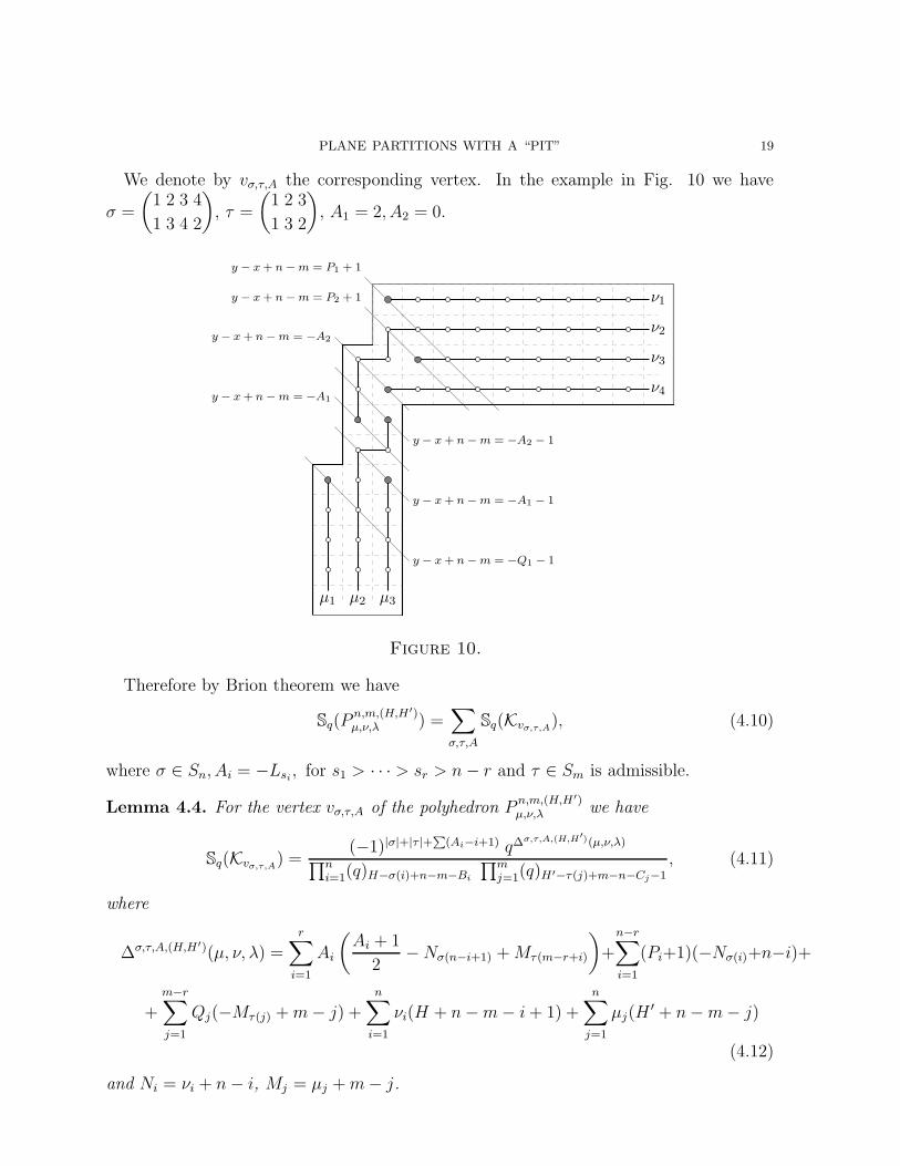
We denote by vσ,τ,A the corresponding vertex. In the example in Fig. 10 we have

σ =

(1 2 3 4

1 3 4 2

), τ =

(1 2 3

1 3 2

), A1 = 2, A2 = 0.

y − x+ n−m = P1 + 1

y − x+ n−m = P2 + 1

y − x+ n−m = −A2

y − x+ n−m = −A1

y − x+ n−m = −A2 − 1

y − x+ n−m = −A1 − 1

y − x+ n−m = −Q1 − 1

ν1

µ1

ν2

µ2

ν3

µ3

ν4

µ4

ν5

µ5

ν6

µ6

ν7

µ7

ν8

µ8

ν9

µ9

ν10

µ10

Figure 10.

Therefore by Brion theorem we have

Sq(Pn,m,(H,H′)µ,ν,λ ) =

∑

σ,τ,A

Sq(Kvσ,τ,A), (4.10)

where σ ∈ Sn, Ai = −Lsi , for s1 > · · · > sr > n− r and τ ∈ Sm is admissible.

Lemma 4.4. For the vertex vσ,τ,A of the polyhedron Pn,m,(H,H′)µ,ν,λ we have

Sq(Kvσ,τ,A) =(−1)|σ|+|τ |+

∑(Ai−i+1) q∆

σ,τ,A,(H,H′)(µ,ν,λ)

∏ni=1(q)H−σ(i)+n−m−Bi

∏mj=1(q)H′−τ(j)+m−n−Cj−1

, (4.11)

where

∆σ,τ,A,(H,H′)(µ, ν, λ) =

r∑

i=1

Ai

(Ai + 1

2−Nσ(n−i+1) +Mτ(m−r+i)

)+

n−r∑

i=1

(Pi+1)(−Nσ(i)+n−i)+

+m−r∑

j=1

Qj(−Mτ(j) +m− j) +n∑

i=1

νi(H + n−m− i+ 1) +n∑

j=1

µj(H′ + n−m− j)

(4.12)

and Ni = νi + n− i, Mj = µj +m− j.


Proof. The proof of this lemma is analogous to the one of Lemma 4.2. In the denominatorwe have a product of (q)h−1 where h is the length of the ribbon. The power of q in thenumerator is made from two summands. The first one

n∑

i=1

νσ(i)(H − σ(i) + (n−m) + 1− Bi) +

m∑

j=1

µτ(j)(H′ − τ(j) +m− n− Cj)

is the sum of the weights of the vertices vi in cones Kvσ,τ,A,i corresponding to ribbons. Thesecond one comes from rewriting 1/(1− q−s) as −qs/(1− qs). Such terms come from theedges of the form −(1, . . . , 1, 0, . . . , 0) as in Lemma 4.2.

It was explained in the proof of Lemma 4.2 that for ribbons which contain boxes (i, H)such terms correspond to the pairs of consecutive boxes s, s+1 such that s+1 is an upperneighbor of the box s. For ribbons which contain boxes (H ′, j) the situation is reflected:if we number boxes from an upper right corner then such terms correspond to the pairsof consecutive boxes s, s+ 1 such that s+ 1 is a left neighbor of the box s.

Moreover, it was explained in the proof of the Lemma 4.3 that such terms corre-spond to the overtaking of the particles, and the corresponding overtakings give theterms

∑ni=1Bi(σ(i) − i) and

∑mj=1Cj(τ(j) − j) (compare with (4.5)). Now for ribbons

which contain boxes (i, H) we have an additional phenomena, namely the particle over-takes standing particles in nonpositive positions (0, . . . ,−H + n+ 1) (except particles inposition −Aj , for j > i). In terms of the proof of the Lemma 4.3 it means that the liney = x−n+m+c for c < 0, can intersect not the first box of another ribbon but vertical bor-der of the diagram (Hn, mH′−n). For each 1 ≤ i ≤ r this gives

∑Ai

s=1 s−∑r

j=i+1(Ai−Aj).The resulting formula is

r∑

i=1

(Ai + 1

2

)+

r∑

i=1

Ai(2i− r − 1) +

n∑

i=1

Bi(σ(i)− i) +m∑

j=1

Cj(τ(j)− j).

Putting all things together and using (4.8), (4.9) we get (4.12) (the sign (−1)∑

Ai−i+1

comes from overtakings of standing particles). �

Now we find χn,mµ,ν,λ(q) as limH,H′→∞ q−∆(H,H′)

Sq(Pn,m,(H,H′)µ,ν,λ ), where

∆(H,H′) =

n−r∑

i=1

νi(H − Pi − i+ n−m) +

m−r∑

j=1

µj(H′ −Qj − j +m− n)

+

n∑

i=n−r+1

νi(H − i+ n−m+ 1) +

m∑

j=m−r+1

µj(H′ − j +m− n).

It is easy to see that ∆σ,τ,A,(H,H′)(µ, ν, λ)−∆(H,H′) = ∆σ,τ ,A(µ, ν, λ) for

σ = σ◦

(1 . . . r r + 1 . . . nn . . . n− r + 1 1 . . . n− r

), τ = τ◦

(1 . . . r r + 1 . . . m

m− r + 1 . . . m 1 . . . m− r

)

and we get formula (2.6). �

4.4. In the previous subsection we proved Theorem 3 under the assumption (4.6)

ν1 > . . . > νn > µ1 > . . . > µm.


But this theorem holds for any ν, µ since it is equivalent to Theorem 1 proven in section 3.In this subsection we explain how to get rid of the condition (4.6) in the context of Briontheorem.

First, note that if some inequalities between νi, µj become equalities then the poly-

hedron Pn,m,(H,H′)µ,ν,λ degenerates. This degeneration changes combinatorial structure, in

particular, some of the vertices merge. But one can ignore this when using Brion theorem(see arguments in [18, Sec. 8]). Therefore Theorem 3 still holds.

Now fix any strong order o on {ν1, . . . , νn, µ1, . . . , µm} such that νi1 > νi2 , µj1 > µj2 fori1 < i2 and j1 < j2. Proposition 4.1 implies that vertices with nonzero contribution to

Sq(Pn,m,(H,H′)µ,ν,λ ) correspond to decompositions of the skew diagram (Hn, mH′−n) − λ into

m+ n ribbons (of which n contain boxes (i, H), 1 ≤ i ≤ n, and m contain boxes (H ′, j),1 ≤ j ≤ m).

The order o provides an additional condition on a such decomposition. The usualpartial order on boxes (bi ≥ bj if bi lies to the northwest of bj) induces a partial orderon ribbons: Ki ≥ Kj if there are boxes bi ∈ Ki, bj ∈ Kj such that bi ≥ bj . Such ordershould be compatible with the order o if we identify ribbons containing (i, H) with νi andribbons containing (H ′, j) with µj .

ν1 > ν2 > µ1 > µ2

ν1

µ1

ν2

µ2

ν3

µ3

ν4

µ4

ν5

µ5

ν6

µ6

ν7

µ7

ν1 > µ1 > ν2 > µ2,ν1 > µ1 > µ2 > ν2

ν1

µ1

ν2

µ2

ν3

µ3

ν4

µ4

ν5

µ5

ν6

µ6

ν7

µ7

ν1 > µ1 > µ2 > ν2,µ1 > ν1 > µ2 > ν2

ν1

µ1

ν2

µ2

ν3

µ3

ν4

µ4

ν5

µ5

ν6

µ6

ν7

µ7

Figure 11. Some examples of decompositions and compatible orders

The set of vertices depends on the order o. But the contribution of a vertex is aproduct of ribbon contributions, and each such contribution is defined for any νi and µj

(not necessarily compatible with o).

So for any given order o the function Sq(Pn,m,(H,H′)µ,ν,λ ) computed using Brion theorem

is defined for any nonnegative integer numbers νi, µj not necessarily compatible with o.

For any given n,m, µ, ν, λ we denote this function just by S(H,H′)o (q) and its limit (as

H,H ′ →∞) as So(q).


Example 4.1. Let n = m = 1, λ = ∅. We have two possible orders o : ν1 > µ1 ando′ : µ1 > ν1. For o we have H ′ − 1 vertices and using Brion Theorem we obtain

S(H,H′)o (q) =

H′−2∑

a=0

(−1)aq(a+12 )q(H+a)ν1+(H′−a−1)µ1

(q)H+a−1(q)H′−a−2

.

For the order o′ we have H − 1 vertices and using Brion Theorem we obtain

S(H,H′)o′ (q) =

H−2∑

b=0

(−1)bq(b+12 )q(H−b−1)ν1+(H′+b)µ1

(q)H−b−2(q)H′+b−1.

These formulas are different, they even have different number of summands. Brion

theorem proves that the first formula calculates Sq(P1,1,(H,H′){µ1},{ν1},∅

) for ν1 > µ1 and the second

formula for µ1 > ν1. But in some cases both formulas work!Namely, using the q-binomial theorem in the form

N∑

c=0

(−1)cq(c2)xc

(q)c(q)N−c

=1

(q)N

N∏

i=1

(1− xqi−1)

for x = qµ1−ν1−H′+2, N = H +H ′− 3 and an obvious observation that right side vanishesfor x = q−d, 0 ≤ d ≤ N − 1 we have

S(H,H′)o (q) = S

(H,H′)o′ (q), for 0 ≤ ν1 − µ1 +H ′ − 2 ≤ H +H ′ − 4.

It is convenient to rewrite the last inequality as

2−H ′ ≤ ν1 − µ1 ≤ H − 2. (4.13)

In this region both formulas give the same (and therefore correct) answer.In the limit H,H ′ → ∞ situation becomes simpler. Indeed, for any given ν1, µ1 and

large enough H,H ′ the inequality (4.13) is satisfied and in the limit So(q) = So′(q).

More generally, we have:

Proposition 4.2. If n + 1 − H ′ ≤ νi − µj ≤ H − m − 1 for any i, j then for any twoorders o, o′ we have

S(H,H′)o (q) = S

(H,H′)o′ (q).

Proof. It is enough to consider the case when the orders o, o′ differ only by an ele-mentary transposition of νi and µj (in o : νi > µj and o′ : µj > νi). Recall that the

summands in S(H,H′)o (q) and S

(H,H′)o′ (q) correspond to decompositions of the skew diagram

(Hn, mH′−n)−λ into m+n ribbons compatible with the orders o and o′ correspondingly.There are three possibilities.

Case 1. Ribbons containing boxes (i, H) and (H ′, j) have no common edges. Corre-

sponding summands appear both in S(H,H′)o (q) and S

(H,H′)o′ (q).

Case 2. Union of ribbons containing boxes (i, H) and (H ′, j) is a ribbon. Denote thisribbon by α − β. Fix ribbons containing other end-boxes (i′, H) and (H ′, j′) for i′ 6= iand j′ 6= j. For such summands α − β is divided by an internal edge e into two ribbonscontaining (i, H) and (H ′, j). Denote by Se,α−β(q) the product of contributions of these


two ribbons. If the edge e is horizontal then the corresponding term appears in S(H,H′)o (q),

otherwise in S(H,H′)o′ (q).

Lemma 4.5. Suppose α− β is a ribbon such that α− β lies in the rectangle H ×H ′ andcontains boxes (i, H) and (H ′, j). If 1 + i−H ′ ≤ ν1 − µ1 ≤ H − j − 1 then

∑

e : horizontal

Se,α−β(q) =∑

e : vertical

Se,α−β(q)

This lemma is a generalization of Example 4.1 and by straightforward calculation re-

duces to the q-binomial theorem. Due to this lemma the contributions to S(H,H′)o (q) and

S(H,H′)o′ (q) are equal to each other in this case.

Example 4.2. Consider α = (4, 2, 1, 1) and β = (1). In this case α − β has 6 internaledges, corresponding decompositions are drawn below in Fig. 12 The terms S1, S2, S4

S1

ν1

µ1S2

ν1

µ1S3

ν1

µ1S4

ν1

µ1S5

ν1

µ1S6

ν1

µ1

Figure 12.

correspond to the horizontal internal edges e and order ν1 > µ1. The terms S3, S5, S6

correspond to the vertical internal edges e and order µ1 > ν1. We have

S1 + S2 − S3 + S4 − S5 − S6 =qµ1+6ν1+4

(q)5−q2µ1+5ν1+2

(q)1(q)4+q3µ1+4ν1+1

(q)2(q)3−

−q4µ1+3ν1+1

(q)3(q)2+q5µ1+2ν1+2

(q)4(q)1−q6µ1+ν1+4

(q)5=qµ1+6ν1+4

(q)5

5∏

i=1

(1− qµ1−ν1−3+i)

So in other words we get zero for −2 ≤ ν1 − µ1 ≤ 2 as in Lemma 4.5.

Case 3. Union of ribbons containing boxes (i, H) and (H ′, j) is a connected skew Youngdiagram α−β but not a ribbon. Informally it means that α−β has width 2 in the middle.In this case there are two ways to decompose α− β into two ribbons. Corresponding two

terms are equal to each other, and one goes to S(H,H′)o (q) and other to S

(H,H′)o′ (q). �

Remark 4.1. The calculation in Case 3 is essentially the last step in the proof of [35,Theorem 2.1] (see our Proposition 4.1).

Tending H,H ′ → ∞ we get from Proposition 4.2 that the function So(q) does notdepend on the order o. For the actual order of νi, µj this function coincides with χn,m

µ,ν,λ(q)and for the order (4.6) this function coincides with right side of (2.6). Hence we provedTheorem 3 for any pair of partitions ν, µ, with l(ν) ≤ n, l(µ) ≤ m.


5. Algebras, representations and resolutions

5.1. For the reference of quantum toroidal algebra U~q(gl1) one can use [14, Sec. 2] or[42], but our notation slightly differs from the loc. cit.5

Fix complex numbers ǫi, where i = 1, 2, 3 viewed as mod 3 residues. We assume thatǫ1 + ǫ2 + ǫ3 = 0. Denote qi = eǫi , ~q = (q1, q2, q3). We assume further that q1, q2, q3 aregeneric, i.e., for integers l, m, n ∈ Z, ql1q

m2 q

n3 = 1 holds only if l = m = n. We set

g(z, w) =3∏

i=1

(z − qiw), κr =3∏

i=1

(qr/2i − q−r/2

i ) =3∑

i=1

(qri − q−ri ), δ(z) =

∑

m∈Z

zm.

The algebra U~q(gl1) is generated by Em, Fm, Hr where m ∈ Z, r ∈ Z \ 0 and invertiblecentral elements C,C⊥. In order to write down the defining relations we form the currents(generating functions of operators)

E(z) =∑

m∈Z

Emz−m, F (z) =

∑

m∈Z

Fmz−m, K±(z) = (C⊥)±1 exp

(∑

r>0

∓κrrH±rz

∓r

).

The relations have form

g(z, w)E(z)E(w) + g(w, z)E(w)E(z) = 0, g(w, z)F (z)F (w) + g(z, w)F (w)F (z) = 0,

K±(z)K±(w) = K±(w)K±(z),g(C−1z, w)

g(Cz, w)K−(z)K+(w) =

g(w,C−1z)

g(w,Cz)K+(w)K−(z),

g(z, w)K±(C(−1∓1)/2z)E(w) + g(w, z)E(w)K±(C(−1∓1)/2z) = 0,

g(w, z)K±(C(−1±1)/2z)F (w) + g(z, w)F (w)K±(C(−1±1)/2z) = 0 ,

[E(z), F (w)] =1

κ1(δ(Cwz

)K+(w)− δ

(Czw

)K−(z)),

Symz1,z2,z3

z2z−13 [E(z1), [E(z2), E(z3)]] = 0, Sym

z1,z2,z3

z2z−13 [F (z1), [F (z2), F (z3)]] = 0.

There exists an action of the group SL(2,Z) on the toroidal algebra U~q(gl1) by auto-morphisms, see [7, Sec. 6.5]. We denote by E⊥

m, F⊥m , H

⊥r images of generators Em, Fm, Hr

after rotation of the lattice clockwise by 90 degrees. Under this rotation C goes to C⊥.Denote by d the operator

[d, Em] = −mEm, [d, Fm] = −mFm, [d,Hr] = −rHr, [d, C] = [d, C⊥] = 0.

This operator introduces the grading on the algebra U~q(gl1). Sometimes it is convenient

to consider d as an additional generator of U~q(gl1). Let V be a representation of U~q(gl1)such that one can define an action of d on the space V with finite dimensional eigenspaces.By the character χ(V ) we denote the trace of the operator D = qd where q is a formalvariable.

5Currently there is no standard convention to the notation, even for the algebra itself other names E ,E1, SH, Uq1,q2,q3(gl1) are also used in the literature.


The algebra U~q(gl1) has the following formal coproduct6

∆(Hr) = Hr ⊗ 1 + C−r ⊗Hr, ∆(H−r) = H−r ⊗ Cr + 1⊗H−r, r > 0

∆(E(z)) = E(C−1

2 z)⊗K+

(C−1

2 z)+ 1⊗ E (z) ,

∆(F (z)) = F (z)⊗ 1 +K−(C−1

1 z)⊗ F (C−1

1 z),

∆(X) = X ⊗X, for X = C,C⊥, D,

(5.1)

where C1 = C ⊗ 1, C2 = 1⊗ C.In all representations of U~q(gl1) considered in this paper we have C⊥ = 1.

In the paper [13] authors defined the MacMahon modules of the algebra U~q(gl1). TheMacMahon modules depend on three partitions µ, ν, λ and two parameters v, c ∈ C

(the central element C acts on these modules as c Id). These modules are denoted byMµ,ν,λ(v, c). The module Mµ,ν,λ(v, c) has the basis |a〉, where a is a plane partitionwhich satisfies condition (1.2). The action of d onMµ,ν,λ(v, c) is defined by d|a〉 = |a||a〉.Therefore the character χ(Mµ,ν,λ(v, c)) is equal to the generating function of plane parti-tions satisfying (1.2).

The modulesMµ,ν,λ(v, c) were originally defined by the explicit formulas for the actionof “rotated” generators E⊥

m, F⊥m , H

⊥r in the basis labeled by plane partitions. For example,

the action of K⊥,±(z) have the form

K⊥,±(z)|a〉 = c1− c−2v/z

1− v/z

∏

(i,j,k)∈a

ψi,j,k(v/z)|a〉 (5.2)

where

ψi,j,k(v/z) =(1− qi−1

1 qj2qk3v/z)(1− q

i1q

j−12 qk3v/z)(1− q

i1q

j2q

k−13 v/z)

(1− qi+11 qj2q

k3v/z)(1− q

i1q

j+12 qk3v/z)(1− q

i1q

j2q

k+13 v/z)

.

Notation (i, j, k) ∈ a means that (i, j, k) belongs to the corresponding 3d Young diagram,see Fig. 1. It is easy to see that the product in the right side of (5.2) becomes finite aftercancellation of common factors, see [13, eq. (3.27)]. The highest weight of Mµ,ν,λ(v, c)is given by the formula (5.2) applied for “minimal” plane partition a satisfying condi-tions (1.2). Note also that here we rather follow [14] then [13] in notations, for example,we include prefactor c in the rational function (5.2).

For generic values c, v, q1, q2, q3 the moduleMµ,ν,λ(v, c) is irreducible. But for c = qn/21 q

m/22

(and generic v, q1, q2, q3) this module has one singular vector. The quotient by the sub-module generated by this vector is irreducible. This quotient is denoted by N n,m

µ,ν,λ(v) andhas the basis |a〉 where a is a plane partition, satisfying both conditions (1.2) and (1.1).Recall that partitions λ, µ, ν satisfy l(ν) ≤ n, l(µ) ≤ m, and λn+1 < m+ 1.

Therefore the character χ(N n,mµ,ν,λ(v)) is equal to the generating function χn,m

µ,ν,λ(q) definedin the introduction. This is the representation theoretic interpretation of the left side of(2.3), (2.4), (2.6). Now we will discuss the representation theoretic interpretation of theright sides.

5.2. It is difficult to write down the explicit action of the generators En, Fn, Hm in themodules N n,m

µ,ν,λ(v). Now we recall a construction of another class of modules, namely,

6Note that our Em, Fm, Hr are called e⊥m, f⊥m, h⊥

r in [14] (up to rescaling of hr).


the Fock modules and intertwining operators between them, which are called screeningoperators. Then we sketch a construction of MacMahon modules N n,m

µ,ν,λ(v) in these terms.

The name of Fock modules over U~q(gl1) comes from the fact that the representationspace is identified with the Fock module over some Heisenberg algebra. In these represen-tations the currents E(z), F (z), K±(z) are given in terms of the Heisenberg algebra (ascombination of vertex operators).

We start from the basic Fock modules F (i)u , where u = ep, p ∈ C and i = 1, 2, 3. The

underlying vector spaces of these representations are modules over a Heisenberg algebrawith generators an, n ∈ Z and relations

[ar, as] = r(q

r/2i − q−r/2

i )3

−κrδr+s,0. (5.3)

The space F (i)u is generated by the highest weight vector v

(i)u such that

arv(i)u = 0 for r > 0; a0v

(i)u = −

ǫ2i p

ǫ1ǫ2ǫ3v(i)u .

Now we define representation ρ(i)u of U~q(gl1) in the space F (i)

u by the formulas

ρ(i)u (E(z)) =u(1− qi)

κ1exp

(∞∑

r=1

q−r/2i κr

r(qr/2i − q−r/2

i )2a−rz

r

)exp

(∞∑

r=1

κr

r(qr/2i − q−r/2

i )2arz

−r

),

ρ(i)u (F (z)) =u−1(1− q−1

i )

κ1exp

(∞∑

r=1

−κr

r(qr/2i − q−r/2

i )2a−rz

r

)exp

(∞∑

r=1

−qr/2i κr

r(qr/2i − q−r/2

i )2arz

−r

),

ρ(i)u (Hr) =ar

qr/2i − q−r/2

i

, ρ(i)u (C⊥) = 1, ρ(i)u (C) = q1/2i ,

ρ(i)u (d)v(i)u = ∆i(p)v(i)u , where ∆i(p) = −

(p+ ǫi)3 − p3

6ǫ1ǫ2ǫ3. (5.4)

Note that generally speaking the operators a0 and d can act on the highest weight

vector v(i)u by any numbers. Our choice is convenient for the formulas below, for example,

the screening operators will commute with d due to our choice.

We formally introduce operators Q by the relation [an, Q] =−ǫ3i

ǫ1ǫ2ǫ3δn,0. This operator

does not act on the spaces F (i)u , but for x ∈ C we define operator exQ : F (i)

u → F(i)qxi u

such

that[an, e

xQ] = 0 for n 6= 0, exQv(i)u = v(i)qxi u.

The U~q(gl1) modules F (i)u are irreducible. In terms of the rotated generators, their

highest weight has the form

K⊥,±(z)v(i)u = q1/2i

1− q−1i u/z

1− u/zv(i)u (5.5)

In particular, the highest weight of the Fock module F (1)u coincides with the highest

weight of the Macmahon module M∅,{ν1},{λ1}(v, c) for c = q1/21 and u = vqλ1

2 qν13 (see

(5.2)). Therefore the irreducible quotient N 1,0∅,{ν1},{λ1}

(v) is isomorphic to the Fock module


F (1)u . Similarly the MacMahon module N 0,1

{µ1},∅,{λ1}t(v) is isomorphic to the Fock module

F (2)u , where u = vqλ1

1 qµ13 .

More generally, we note that the highest weight of the module N n,mµ,ν,λ(v) is given by the

rational function, see [13, eq. (3.27)]. Numbers of zeros and poles in this rational functionare equal, positions of zeros and poles of this rational function differs by the factors ofthe form qi1q

j2q

k3 , i, j, k ∈ Z, therefore it can can be decomposed as the product of several

factors of the type (5.5). Therefore N n,mµ,ν,λ(v) is isomorphic to a subquotient of a tensor

product of Fock module

F (i1)u1⊗ F (i2)

u2⊗ · · · ⊗ F (ik)

uk.

Here we used the fact that the action of K⊥,±(z) on the tensor product of highest vectorsis given by the product of rational functions (5.5) by [15, Lemma A.9] (or conjugacy ofcoproducts ∆ and ∆⊥ [15, Lemma A.13]). Clearly such tensor product is also a Fockrepresentation of the sum of k copies of the Heisenberg algebras or, in other words,Heisenberg algebra with generators ar,i, r ∈ Z, 1 ≤ i ≤ k. Now we will describe the image

of U~q(gl1) in these representations.

5.3. First, we consider the tensor product F (i)u1 ⊗F

(i)u2 . This tensor product was essentially

elaborated in [17] which we follow. We introduce the Heisenberg generators hn, n 6= 0

acting on F (i)u1 ⊗F

(i)u2

h−r = q−ri (a−r ⊗ 1)− q−r/2

i (1⊗ a−r), hr = qr/2i (ar ⊗ 1)− qri (1⊗ ar), r > 0. (5.6)

For any n ∈ Z \ {0} they satisfy [hn,∆(Hm)] = 0 for all m ∈ Z \ {0} and, clearly, hnis a unique (up to a normalization) linear combination of an ⊗ 1 and 1 ⊗ an with suchproperty. In our normalization we have

[hr, hs] = r(qri − q

−ri )(q

r/2i − q−r/2

i )2

−κrδr+s,0.

Denote Q1 = Q ⊗ 1, Q2 = 1 ⊗ Q, Q12 = Q1 − Q2, a12 = a0 ⊗ 1 − 1 ⊗ a0, u1 = ep1,u2 = ep2 . Following [40], [11] we introduce two screening currents

Sii+(z) = e

ǫi+1ǫi

Q12zǫi+1ǫi

a12+ǫi

ǫi−1 exp

(∞∑

r=1

−(qr/2i+1−q−r/2i+1 )

r(qr/2i −q

−r/2i )

h−rzr

)exp

(∞∑

r=1

(qr/2i+1−q

−r/2i+1 )

r(qr/2i −q

−r/2i )

hrz−r

)

Sii−(z) = e

ǫi−1ǫi

Q12zǫi−1ǫi

a12+ǫi

ǫi+1 exp

(∞∑

r=1

−(qr/2i−1−q−r/2i−1 )

r(qr/2i −q

−r/2i )

h−rzr

)exp

(∞∑

r=1

(qr/2i−1−q

−r/2i−1 )

r(qr/2i −q

−r/2i )

hrz−r

).

(5.7)

Lemma 5.1. The following screening operators

Sii+ =

∮Sii+(z)dz, Sii

− =

∮Sii−(z)dz. (5.8)

commute with action of U~q(gl1) (including the operator d).

Here∮is an integral over small contour around 0 (residue at 0). This integral is defined

if the corresponding power of z is integer. In other words the operator Sii+ acts on the


tensor product F (i)u1 ⊗ F

(i)u2 if and only if p2−p1+ǫi

ǫi−1(eigenvalue of ǫi+1

ǫia12 +

ǫiǫi−1

) is integer

and similarly for Sii−. The lemma follows from a direct computation, which is given for

example in [40] or in [11, Sec. 5] in the equivalent setting of deformed Virasoro (and,more generally, deformed W algebras).

Note that the screening currents formally commute

Sii+(z)S

ii−(w) =

1

(z − q−1/2i w)(z − q1/2i w)

:Sii+(z)S

ii−(w):= Sii

−(w)Sii+(z).

Here and below, :· · ·: is a standard Heisenberg normal ordering, in which ar appears tothe right of a−r, r > 0, and a0 appears to the right of Q.

We denote by W~q(gl2) the quotient of U~q(gl1) by the two-sided ideal generated by

operators, which act as 0 on any tensor product F (i)u1 ⊗F

(i)u2 . It was proven in [17, Sec. 2.4]

that this W -algebra is just the product of a Heisenberg algebra and a deformed Virasoroalgebra introduced in [40], in other words product of W~q(gl1) and W~q(sl2), as expected.

Now on can use the results on the representation theory of deformed Virasoro algebra

for the study of representation F (i)u1 ⊗ F

(i)u2 .

7 For generic u1, u2 this module is irreducible.But if u2 = u1q

si+1q

ti−1 where s, t ∈ Z and st > 0 then it is not so. If s, t < 0, then

F (i)u1 ⊗ F

(i)u2 has a singular vector and this singular vector can be obtained by the action

of the power of screening operator Sii+ or Sii

− [40, Sec. 5]. The quotient of F (i)u1 ⊗ F

(i)u2

by the submodule generated by this singular vector is irreducible.8 The highest weight

of this irreducible quotient coincides with the highest weight of F (i)u1 ⊗ F

(i)u2 and actually

coincides with the highest weight of N 2,0∅,{ν1,ν2},{λ1,λ2}

(v). Since the MacMahon module

N 2,0∅,{ν1,ν2},{λ1,λ2}

(v) is also irreducible we proved that it is isomorphic to the quotient of

F (i)u1 ⊗F

(i)u2 . This can be written as a short exact sequence.

The simplest example of such complex is given if s or t equal to 1

0→ F (1)

vqλ12 q

ν1−13

⊗ F (1)

vqλ1−s

2 qν13

S11−−−→ F (1)

vqλ12 q

ν13

⊗F (1)

vqλ1−s

2 qν1−13

→ N 2,0∅,{ν1,ν1},{λ1,λ1−s+1}(v)→ 0

0→ F (1)

vqλ1−12 q

ν13

⊗ F (1)

vqλ12 q

ν1−s

3

S11+−−→ F (1)

vqλ12 q

ν13

⊗F (1)

vqλ1−12 q

ν1−s

3

→ N 2,0∅,{ν1,ν1−s+1},{λ1,λ1}

(v)→ 0

.

For a generic module N 2,0∅,{ν1,ν2},{λ1,λ2}

(v) the corresponding short exact sequences have the

form

0→ F (1)

vqλ12 q

ν2−13

⊗F (1)

vqλ2−12 q

ν13

(S11− )ν1−ν2+1

−−−−−−−→ F (1)

vqλ12 q

ν13

⊗F (1)

vqλ2−12 q

ν2−13

→ N 2,0∅,{ν1,ν2},{λ1,λ2}

(v)→ 0

0→ F (1)

vqλ2−12 q

ν13

⊗ F (1)

vqλ12 q

ν2−13

(S11+ )λ1−λ2+1

−−−−−−−−→ F (1)

vqλ12 q

ν13

⊗F (1)

vqλ2−12 q

ν2−13

→ N 2,0∅,{ν1,ν2},{λ1,λ2}

(v)→ 0

,

(5.9)where operators (S11

± )r should be considered as r-fold integrals over the appropriate cyclewith the appropriate additional (Lukyanov) factor (see [25]). Now we compute the Euler

7instead of this one can use [9] but the coproduct in loc. cit. is different from (5.1) used in our paper.8This follows from the irreducibility of the quotient in conformal limit q1, q2, q3 → 1, where deformed

Virasoro algebra becomes Virasoro algebra and one can use e.g. [12, Theorem 1.9(ii)]


characteristic of (5.9). Using χ(F (1)u1 ⊗F

(1)u2 ) = q∆1(p1)+∆1(p2)/(q)2∞, where ∆i(p) is defined

in (5.4) we have

χ(N 2,0

∅,{ν1,ν2},{λ1,λ2}(v))= q∆

q−(λ1+1)(ν1+1)−λ2ν2 − q−(λ1+1)ν1−λ2(ν2+1)

(q)2∞, (5.10)

where

∆ = ∆1(p+ λ1ǫ2 + ν1ǫ3) + ∆1(p+ (λ2 − 1)ǫ2 + (ν2 − 1)ǫ3) + (λ1 + 1)(ν1 + 1) + λ2ν2,

and ep = v. Up to the factor q... the formula (5.10) coincides with (2.6) (or with its specialcase (1.4)).

In a similar manner one can construct resolutions of N 0,2{µ1,µ2},∅,{λ1,λ2}t

(v) in terms of

F (2)u1 ⊗ F

(2)u2 .

Below we will discuss the algebra of screening operators which commute with the image

of algebra U~q(gl1) in the representation F (1)u1 ⊗. . .⊗F

(1)un . This system of screening operators

coincides with the one studied in [11], the image of U~q(gl1) commutes with them and is

denoted by W~q(gln). We conjecture that one can construct resolutions of N n,0∅,ν,λ(v) in

terms of the modules F (1)u1 ⊗ . . .⊗ F

(1)un . See Section 5.5 for more details.

5.4. Second, we consider the tensor product F (1)u1 ⊗ F

(2)u2 . We introduce the Heisenberg

generators hn acting on F (1)u1 ⊗F

(2)u2 as follows

h−r =q−r1 (q

r/22 − q−r/2

2 )

qr/21 − q−r/2

1

(a−r ⊗ 1)−q−r/21 (q

r/21 − q−r/2

1 )

qr/22 − q−r/2

2

(1⊗ a−r),

hr =qr/21 (q

r/22 − q−r/2

2 )

qr/21 − q−r/2

1

(ar ⊗ 1)−q−r/23 (q

r/21 − q−r/2

1 )

qr/22 − q−r/2

2

(1⊗ ar),

r > 0. (5.11)

For any n ∈ Z \ {0} they satisfy [hn,∆(Hm)] = 0 for all m ∈ Z \ {0} and, clearly, hnis a unique (up to a normalization) linear combination of an ⊗ 1 and 1 ⊗ an with suchproperty. In our normalization we have

[hr, hs] = rδr+s,0.

Similarly to the previous case, denote Q1 = Q⊗ 1, Q2 = 1⊗ Q, a1 = a0 ⊗ 1, a2 = 1⊗ a0,u1 = ep1 , u2 = ep2 and introduce a screening current

S12(z) = eǫ2ǫ1

Q1−ǫ1ǫ2

Q2zǫ2ǫ1

a1−ǫ1ǫ2

a2+ǫ2ǫ3 exp

(∞∑

r=1

1

−rh−rz

r

)exp

(∞∑

r=1

1

rhrz

−r

). (5.12)

Lemma 5.2. The following screening operator

S12 =

∮S12(z)dz. (5.13)

commutes with action of U~q(gl1) (including the operator d).

About the meaning of the integration see the comment after the Lemma 5.1. The proofof the lemma is similar to the one of the Lemma 5.1 and based on a standard computation.


Proof. Clearly the action of ∆(K±(z)) commutes with whole current S12(w) since thelatter is expressed in terms of hn. Now we show that ∆(E(z)) commutes with S12.

DenoteΛ1(z) = E

(q−12 z)⊗K+

(q−12 z), Λ2(z) = 1⊗ E (z) .

Then ∆(E(z)) = Λ1(z) + Λ2(z). We have

Λ1(z)S12(w) = q2

1− w/z

1− q2w/z:Λ1(z)S

12(w):, S12(w)Λ1(z) =1− z/w

1− q−12 z/w

:Λ1(z)S12(w):

Λ2(z)S12(w) = q−1

1

1− w/z

1− q−11 w/z

:Λ2(z)S12(w):, S12(w)Λ2(z) =

1− z/w

1− q1z/w:Λ2(z)S

12(w):

Therefore we have[Λ1(z), S

12(w)]= (q2 − 1)δ

(q−12 z

w

):Λ1(z)S

12(w):= (q2 − 1) :Λ1(z)S(q−12 z): δ

(q−12 z

w

)

[Λ2(z), S

12(w)]= (q−1

1 − 1)δ(q1zw

):Λ2(z)S

12(w):= (q−11 − 1) :Λ2(z)S

12(q1z): δ(q1zw

).

Finally we get

[Λ1(z) + Λ2(z), S

12(w)]= Dq3

(w(q2 − 1) :Λ1(z)S

12(q−12 z): δ

(q−12 z

w

)),

where we used

(1− q2) :Λ1(z)S12(q−1

2 z):= q2(1− q1) :Λ2(z)S12(q1z):

and notation [Daf ](w) =f(w)−f(wa)

w. Therefore ∆(E(z)) commutes with S12 =

∮S12(z)dz,

the computation for ∆(F (z)) is similar. �

Note that in this case we have only one screening current contrary to two currentsSii−(z), S

ii+(z) above in (5.7). Also note that the commutation relations of S12(z) do not

depend on q1, q2, q3, namely

S12(z)S12(w) = (z − w) :S12(z)S12(w):= −S12(w)S12(z).

In other words, we have a “fermionic” screening current. In particular, we have S12S12 = 0.We denote by W~q(gl1|1) the quotient of U~q(gl1) by the two-sided ideal generated by

operators, which act as 0 on any tensor product F (1)u1 ⊗ F

(2)u2 . The arguments for such

name will be given below.

For generic u1, u2 the module F (1)u1 ⊗ F

(2)u2 is irreducible. But in the resonance case we

have nontrivial intertwining operators between such modules and can construct a complexwith cohomology N 1,1

{µ1},{ν1},∅(v).

There are two infinite exact sequences

. . .S12

−−→ F (1)

vq−22 q

ν13

⊗F (2)

vq31qµ13

S12

−−→ F (1)

vq−12 q

ν13

⊗F (2)

vq21qµ13

S12

−−→ F (1)

vqν13⊗F (2)

vq1qµ13→ N 1,1

{µ1},{ν1},∅(v)→ 0,

(5.14)

0→ N 1,1{µ1},{ν1},∅

(v)S12

−−→ F (1)

vq2qν13⊗F (2)

vqµ13

S12

−−→ F (1)

vq22qν13⊗F (2)

vq−11 q

µ13

S12

−−→ F (1)

vq32qν13⊗F (2)

vq−21 q

µ13

S12

−−→ . . .

(5.15)Of course, the exactness is nontrivial, the proof will be given elsewhere.


Now we calculate the Euler characteristics of the exact sequence (5.14). Introduce p byep = v and ∆ = ∆1(p + ν1ǫ3) + ∆2(p + ǫ1 + µ1ǫ3). We have an algebraic identity (usingthe definition (5.4))

∆1(p+ν1ǫ3−aǫ2) + ∆2(p+(a+1)ǫ1+µ1ǫ3)−∆ =

(a+ 1

2

)+ (ν1 − µ1)a.

Therefore

χ(N 1,1

{µ1},{ν1},∅(v))= q∆R(ν1 − µ1; q) (5.16)

where function R is defined in (2.2). Up to a factor q... this formula coincides with (2.6)for the special case n = m = 1.

Similarly, computing the Euler characteristic of the exact sequence (5.15) one gets

χ(N 1,1

{µ1},{ν1},∅(v))= q∆1(p+ν1ǫ3+ǫ2)+∆2(p+µ1ǫ3)R(µ1 − ν1; q).

Of course, the fact that R(ν1−µ1; q) and R(µ1− ν1; q) are proportional is not surprising,it is equivalent to proportionality of χ1,1

µ1,ν1,∅(q) and χ1,1ν1,µ1,∅(q), which follows from the

bijection given by transposition of plane partition a. See also example 4.1 above.

5.5. Now we want to consider tensor products

F (1)u1⊗ . . .⊗F (1)

un⊗ F (2)

un+1⊗ . . .⊗ F (2)

un+m. (5.17)

Similarly to previous discussion we expect that the MacMahon module N n,mµ,ν,λ(v) admits

a resolution consisting of modules of the type (5.17). For example one can easily see that

the central charge of N n,mµ,ν,λ(v) and central charge of (5.17) are both equal to c = q

n/21 q

m/22 .

Moreover we can consider another ordering in the tensor product (5.17). For generic

parameters u any tensor product of n modules F (1)ui and m modules F (2)

uj is isomorphic to

the product in the ordering (5.17). For each pair of neighbor Fock modules F (il)ul ⊗F

(il+1)ul+1

we constructed above the screening operators(Silil+1∗

)l,l+1

, where indices l, l+1 label Fock

modules in which this operator acts and ∗ = ± if il = il+1, while ∗ should be ignored

when il 6= il+1. For any l, ∗ the operator(Silil+1∗

)l,l+1

commutes with U~q(gl1).

For modules (5.17) it is convenient to decompose the corresponding screening operatorsinto 3 systems:

S1 ={(S11−

)i,i+1|0 < i < n

},

S2 ={(S22+

)j,j+1|n < j < n+m

},

S3 ={(S11+

)i,i+1

,(S12)n,n+1

,(S22−

)j,j+1|0 < i < n, n < j < n+m

}.

(5.18)

We will denote by W~q(gln|m) the quotient of U~q(gl1) by the two-sided ideal generatedby operators, which act as 0 on any tensor product (5.17).

Now we discuss a representation theoretic interpretation of the character formulas (2.6),(2.4), (2.3).• Each term in the sum of right side of (2.6) has the form of q∆/(q)n+m

∞ . This is thecharacter of the Fock module (5.17). Therefore it is natural to expect that right side


of (2.6) is an Euler characteristic of a resolution, consisting of Fock modules (5.17). Theterms in this resolution should be labeled by (σ, τ, A) ∈ Θ as in (2.6). We will say thatthis resolution is a materialization of the formula (2.6).

This resolution of W~q(gln|m) modules is a generalization of resolutions (5.9) and (5.14),(5.15) discussed above. The intertwining operators in this resolution could be constructedusing screening operators. The construction of such resolution is unknown (actually wedid not give a proof of the existence of (5.9) and (5.14),(5.15) but these particular casesare rather easy).

Even in the case m = 0 which corresponds to W~q(gln) we did not find this resolution

in the literature. For the construction of intertwining operators in the W~q(gln) case see[16].

• The algebra U~q(gl1) acts on the product of first n factors of (5.17) through the

quotient W~q(gln) and acts on the product of last m factors of (5.17) through the quotient

W~q(glm). Therefore the coproduct ∆: U~q(gl1)→ U~q(gl1)⊗U~q(gl1) provides an embedding

W~q(gln|m) → W~q(gln) ⊗ W~q(glm). The latter algebra has representations of the form

N n,0∅,ν,ν(v1) ⊗ N

0,mµ,∅,µ(v2). Since the character of each factor is given by formula (1.4) we

have

χ(N n,0∅,ν,ν(v1)⊗N

0,mµ,∅,µ(v2)) = q∆

aν+ρ(q−ν−ρ)aµ+ρ(q

−µ−ρ)

(q)n+m∞

,

for certain ∆. The right side of the character formula (2.4) is a linear combination of suchterms. Therefore it is natural to expect that there exists a resolution ofN n,m

µ,ν,λ(v) consisting

of modules N n,0∅,ν,ν(v1)⊗N

0,mµ,∅,µ(v2) with the cohomology N n,m

µ,ν,λ(v). This resolution shouldbe a materialization of the character formula (2.4). See also Section 5.7 below.• Consider tensor product

F (1)u1⊗. . .⊗F (1)

un−r⊗F (2)

un−r+1⊗. . .⊗F (2)

un+m−2r⊗(F (1)

un+m−2r+1⊗F (2)

un+m−2r+2⊗. . .⊗F (1)

un+m−1⊗F (2)

un+m

).

(5.19)As mentioned before this product is isomorphic to (5.17) (for generic parameters ul).

The algebra U~q(gl1) acts on the product (5.19) through the algebra W~q(gl1)⊗(n+m−2r)⊗W~q(gl1|1)

⊗r,

where W~q(gl1)⊗n+m−2r is by definition just Heisenberg algebra acting on the first n+m−2r

factors of (5.19). Therefore W~q(gln|m) is a subalgebra of W~q(gl1)⊗n+m−2r ⊗W~q(gl1|1)

⊗r.The latter W -algebra has representations

F (1)u1⊗. . .⊗F (1)

un−r⊗F (2)

un−r+1⊗. . .⊗F (2)

un+m−2r⊗N 1,1

{m1},{n1},∅(v1)⊗. . .⊗N

1,1{mr},{nr},∅

(vr). (5.20)

Due to (5.16) the character of these representations are equal to∏r

i=1R(di; q)·q∆/(q∞)m+n−2r,

where di = ni −mi and ∆ is specified by parameters uivi, mi, ni.If we compute the determinant in right side of (2.3) we get the linear combination of

terms∏r

i=1R(di; q) · q∆/(q∞)m+n−2r as before. Therefore it is natural to conjecture the

existence of the resolution of N n,mµ,ν,λ(v) consisting of modules of the type (5.20). And this

resolution should be a materialization of the character formula (2.3).

Remark 5.1. One can consider generic tensor product,

F (1)u1⊗ · · · ⊗ F (1)

un⊗ F (2)

un+1⊗ · · · ⊗ F (2)

un+m⊗ F (3)

un+m+1⊗ · · · ⊗ F (3)

un+m+k.


The quotient of U~q(gl1) by the two-sided ideal generated by operators, which act as 0 onany such tensor product is a certain W algebra depending on three integer parametersk, n,m. These algebras (or, rather, their conformal limits) appear recently in [31], [22] ina different context, the formulas for screening operators for these algebras follows fromthe Lemmas 5.1, 5.2. We hope to study these algebras in more details elsewhere.

5.6. Now we consider the conformal limit of the previous constructions. We rescaleǫi → ~ǫi, pl → ~pl and then send ~ to zero, i.e., send all parameters qi, ul to 1 with acertain speed. Now consider the limit of screening operators, we will see that this limit iswell defined.

Let Cn+m be a vector space with the scalar product (·, ·) given in orthogonal basis elby the formula

(ei, ei) = −ǫ21ǫ2ǫ3

, (ej , ej) = −ǫ22ǫ1ǫ3

, 1 ≤ i ≤ n, n+ 1 ≤ j ≤ n +m.

Denote by an,l, n 6= 0 the limit of generators an acting on the l-th factor in (5.17). Asthe limit of (5.3) we get

[ar,i, as,j] = −r(ei, ej)δr+s,0.

By Ql we denote is a limit of Ql, and by a0,l we denote

a0,i = lim~→0

a0,i− iǫ21ǫ2ǫ3

, a0,j = lim~→0

a0,j −nǫ2ǫ3− (j−n)

ǫ22ǫ1ǫ3

, 1 ≤ i ≤ n, n+1 ≤ j ≤ n+m,

here such strange shifts are introduced in order to hide factors like zǫ2/ǫ3 in the definitionof S12 in (5.12). Anyway, we get a relation [a0,l, Ql′ ] = (el, el′). As before, the operator

Ql does not act on any Fock module but the exponent exQl acts from one Fock module toanother shifting the eigenvalue of a0,l.

It is convenient to introduce

ϕl(z) =∑

r∈Z\0

ar,lrz−r + a0,l log z + Ql, (5.21)

Then, the limits of screening currents have the form

lim~→0

(S11± (z))i,i+1 =:exp

(∑n+m

l=1(α±,i)lϕl(z)

):, 0 < i < n,

lim~→0

(S12(z))n,n+1 =:exp(∑n+m

l=1(αn)lϕl(z)

):,

lim~→0

(S22± (z))j,j+1 =:exp

(∑n+m

l=1(α±,j)lϕl(z)

):, n < j < n+m.

We consider α±,i, αn, α±,j as the vectors in Cn+m which have the form

α+,i =ǫ2ǫ1ei −

ǫ2ǫ1ei+1, αn =

ǫ2ǫ1en −

ǫ1ǫ2en+1, α−,j =

ǫ1ǫ2ej −

ǫ1ǫ2ej+1

α−,i =ǫ3ǫ1ei −

ǫ3ǫ1ei+1, α+,j =

ǫ3ǫ2ej −

ǫ3ǫ2ej+1.

Slightly abusing notation we will say that α ∈ SI , for I = 1, 2, 3 if the correspondingscreening operator belongs to SI .


For any β, γ ∈ Cn+m the commutation relations of vertex operators have the form

:exp(∑n+m

l=1βlϕl(z)

): · :exp

(∑n+m

l=1γlϕl(w)

):

= (z − w)(β,γ) :exp(∑n+m

l=1βlϕl(z) + γlϕl(w)

): .

In particular, if (β, γ) ∈ 2Z then the corresponding vertex operators formally commuteand if (β, γ) ∈ 2Z+1 then the corresponding vertex operators formally anticommute. It iseasy to see that if two vectors α, α′ belong to different systems S then the scalar product(α, α′) ∈ Z, i.e., corresponding screening operators formally commute or anticommute.The Gramian matrices for vectors from S1,S2,S3 are given below

S1 :

−2ǫ3ǫ2

ǫ3ǫ2

0 . . . 0

ǫ3ǫ2

−2ǫ3ǫ2

. . .. . .

...

0. . .

. . .. . . 0

.... . .

. . . −2ǫ3ǫ2

ǫ3ǫ2

0 . . . 0 ǫ3ǫ2

−2ǫ3ǫ2

, S2 :

−2ǫ3ǫ1

ǫ3ǫ1

0 . . . 0

ǫ3ǫ1

−2ǫ3ǫ1

. . .. . .

...

0. . .

. . .. . . 0

.... . .

. . . −2ǫ3ǫ1

ǫ3ǫ1

0 . . . 0 ǫ3ǫ1

−2ǫ3ǫ1

,

S3 :

−2ǫ2ǫ3

ǫ2ǫ3

0 . . . 0 . . . . . . . . . 0

ǫ2ǫ3

−2ǫ2ǫ3

. . .. . .

......

0. . .

. . .. . . 0

......

. . .. . . −2ǫ2

ǫ3ǫ2ǫ3

. . ....

0 . . . 0 ǫ2ǫ3

1 ǫ1ǫ3

0 . . . 0...

. . . ǫ1ǫ3

−2ǫ1ǫ3

. . .. . .

...... 0

. . .. . .

. . . 0...

.... . .

. . . −2ǫ1ǫ3

ǫ1ǫ3

0 . . . . . . . . . 0 . . . 0 ǫ1ǫ3

−2ǫ1ǫ3

.

The Gramian matrix corresponding to S1 is equal to the Cartan matrix of sln multi-plied by − ǫ3

ǫ2. Let us recall what commutes with the corresponding screening operators.

First, note that operators ar,j, n + 1 ≤ j ≤ n +m, clearly commutes with these screen-ing operators, the nontrivial part of centralizer is written in terms of other generators.Namely, it was proven in [10] that W -algebra W(sln) is a centralizer of such screeningoperators in the Heisenberg vertex algebra with generators ar,i−ar,i+1, 1 ≤ i < n, the pa-rameter − ǫ3

ǫ2is responsible for central charge. The additional Heisenberg operators

∑ar,i

also commutes with these screening operators, therefore the centralizer in the Heisenbergvertex algebra with generators ar,i, 1 ≤ i ≤ n coincides with W(gln) [32].

Similarly, the centralizer of screening operators from S2 the Heisenberg vertex algebrawith generators ar,j, n+ 1 ≤ j ≤ n+m coincides with W(glm).

The Gramian matrix corresponding to S3 has blocks corresponding to sln, slm and oneadditional column and row between them. This additional column and row corresponds


to additional vector in S3 which corresponds to fermionic screening operator. Thereforewe call the W -algebra commuting with this system W(gln|m). The W(gln|1) case wasconsidered in [21], but we did not find any reference for general n,m. Note that ourW -algebras differ from the ones introduced in [27].

We expect that resolutions conjectured in Section 5.5 have conformal limit. We discusstheir quantum group meaning in the next section.

5.7. A standard statement (conjecture) in the theory of vertex algebras is an equivalenceof the abelian categories of certain representations of a vertex algebra and certain rep-resentations of a quantum group. This is a statement similar to the Drinfeld–Kohno orKazhdan–Lusztig theorems [26]. In fact, this equivalence of categories is an equivalenceof braided tensor categories, but we do not need tensor structure here.

It is widely believed that a certain category of representations of the vertex alge-bra W(gln) is equivalent to a certain category of representations of the quantum groupUqgln ⊗ Uq′gln, where parameters q, q′ are given in terms of ǫ1, ǫ2 (people also use modu-lar double of Uqgln). We conjecture that the same relation holds for the vertex algebra

W(gln|m) and the quantum group Uqgln|m ⊗ Uq′gln ⊗ Uq′′glm for certain q, q′, q′′ given interms of ǫ1, ǫ2.

Denote by L(n)ν the finite dimensional irreducible representation of Uq′(gln), recall that

these representations are labeled by partitions ν such that l(ν) ≤ n. Similarly denote by

L(m)µ the finite dimensional irreducible representation of Uq′′glm.For Uqgln|m we will consider two types of representations. It is known (see [4], [39]) that

irreducible Uqgln|m submodules of the tensor powers of Cn|m are labeled by partitions λsuch that λn+1 < m + 1, such irreducible modules are called tensor representation. We

denote an analogous representation of Uqgln|m by L(n|m)λ . Let p ⊂ gln|m be a parabolic

subalgebra with a Levi subgroup gln⊕glm. The algebra p acts on a tensor product of finitedimensional representations of gln and glm and a corresponding induced gln|m module iscalled Kac module. We denote an analogues representation for Uqgln|m by Vν,µ, where ν, µlabel the finite dimensional representations of gln and glm correspondingly.

We conjecture that under the aforementioned equivalence the tensor product of irre-

ducible modules L(n|m)λ ⊗ L(n)

ν ⊗ L(m)µ goes to the conformal limit of N n,m

µ,ν,λ(v), and tensor

product Vν,µ ⊗ L(n)ν ⊗ L

(m)µ goes to the conformal limit of N n,0

∅,ν,ν(v1)⊗N0,mµ,∅,µ(v2).

9

In paper [8] Cheng, Kwon and Lam constructed a resolution in terms of the Kac modulesof the tensor module of gln|m. Taking the (conjectural) q-deformation of this resolution we

have a complex which consists of modules Vν,µ with the cohomology L(n|m)λ . Multiplying

by L(n)ν ⊗L

(m)µ we get a complex of Uqgln|m⊗Uq′gln⊗Uq′′glm modules. Then, applying the

above equivalence we get a resolution of the conformal limit of N n,mµ,ν,λ(v) in terms of the

conformal limits of N n,0∅,ν,ν(v1)⊗N

0,mµ,∅,µ(v2). This resolution should be a materialization of

(2.4), its q-deformation was discussed above in Section 5.5.

9Here we are a bit sloppy about parameter v in Nn,mµ,ν,λ(v), actually partition ν in L

(n)ν can consist of

non integer parts with integer differences (instead of ν in Nn,mµ,ν,λ(v)) and total shift of these parts depends

on v.


The Euler characteristic of the resolution constructed in [8] yields the following formula

sλ(x|y) =∑

α1≥α2≥...≥αr≥r−m

(−1)∑

αisπ+m−r,−α(x)sα,κ(y)∏

1≤i≤n,1≤j≤m

(1 +

yjxi

).

Here the notation π, κ were introduced in Section 2.1, sµ(x) is a Schur polynomial, i.e.,

the character of L(m)µ and sλ(x|y) is a hook Schur polynomial (or super-Schur polynomial),

i.e., the character of L(n|m)λ . This formula resembles our character formula (2.4).

Remark 5.2. Moens and van der Jeugt in the paper [37] found another formula for the

character of L(n|m)λ

sλ(x|y) =

(−1)mn−r∏i,j

(1 +

yjxi

)

V (x1, . . . , xn)V (y1, . . . , ym)det

(∑a≥0

(−1)ax−a−1+mj yai

)

1≤i≤m1≤j≤n

(yQj

i

)1≤i≤m

1≤j≤m−r(xPi+mj

)1≤i≤n−r1≤j≤n

0

.

(5.22)This formula is similar to our formula (2.3). It is natural to conjecture that there is aresolution which is a materialization of (5.22) and under the equivalence this resolutiongoes to a resolution which is a materialization of (2.3).

References

[1] M. Aigner, Lattice Paths and Determinants Computational Discrete Mathematics, 112, LectureNotes in Comput. Sci., 2122, Springer-Verlag, Berlin, (2001).

[2] A. Barvinok Integer points in polyhedra EMS, Zurich, 2008.[3] M. Beck, C. Haase, F. Sottile, Formulas of Brion, Lawrence, and Varchenko on rational generating

functions for cones, Math. Intelligencer 31 1(2009), 9–17; [arXiv:math/0506466].[4] A. Berele, A. Regev, Hook Young diagrams with applications to combinatorics and representations

of Lie superalgebras, Adv. Math., 64, (1987), 118–175.[5] I.N. Bernstein, I.M. Gelfand, S.I. Gelfand, Differential operators on the base affine space and a study

of g-modules, I.M. Gelfand (ed.), Lie groups and their representations, Proc. Summer School onGroup Representations, Janos Bolyai Math. Soc.& Wiley (1975), 39–64.

[6] M. Brion, Points entiers dans les poly‘edres convexes, Ann. Sci. Ecole Norm. Sup. 21 4 (1988),653663.

[7] I. Burban, O. Schiffmann On the Hall algebra of an elliptic curve Duke Math. J. 161 7 (2012),11711231; [arXiv:math/0505148].

[8] Shun-Jen Cheng, Jae-Hoon Kwon, Ngau Lam, A BGG-Type Resolution for Tensor Modules over

General Linear Superalgebra, Lett. Math. Phys., 84 1, (2008), 75–87; [arXiv:0801.0914].[9] B. Feigin, E. Feigin, M. Jimbo, T. Miwa, E. Mukhin, Quantum continuous gl∞: Tensor product of

Fock modules and Wn characters, Kyoto J. Math., 51 2, (2011) 365–392; [arXiv:1002.3113].[10] B. Feigin, E. Frenkel, Affine Kac-Moody algebras at the critical level and Gelfand-Dikii algebras, Int.

Jour. Mod. Phys. A7, Supplement 1A (1992) 197–215.[11] B. Feigin, E. Frenkel, Quantum W-algebras and Elliptic Algebras, Comm. Math. Phys., 178 3,

(1996), 653–677; [arXiv:q-alg/9508009].[12] B. Feigin and D. Fuchs, Representations of the Virasoro algebra. Representations of Lie Groups and

Related Topics, 465, Adv. Stud. Contemp. Math., 7, Gordon and Breach, New York, 1990.[13] B. Feigin, M. Jimbo, T. Miwa, E. Mukhin, Quantum toroidal gl1 algebra: plane partitions, Kyoto J.

Math., 52 3, (2012), 621–659; [arXiv:1110.5310].[14] B. Feigin, M. Jimbo, T. Miwa, E. Mukhin, Quantum toroidal gl1 and Bethe ansatz, J.Phys. A48 24,

(2015), 244001; [arXiv:1502.07194].

http://arxiv.org/abs/math/0506466


http://arxiv.org/abs/0801.0914


http://arxiv.org/abs/q-alg/9508009




[15] B. Feigin, M. Jimbo, T. Miwa, E. Mukhin, Finite type modules and Bethe Ansatz for quantum

toroidal gl(1); Comm. Math. Phys. 356 1 (2017), 285–327; [arXiv:1603.02675].[16] B. Feigin, M. Jimbo, T. Miwa, A. Odesskii, Ya. Pugai, Algebra of screening operators for the deformed

Wn algebra, Comm. Math. Phys., 191 (3), (1998), 501–541; [arXiv:q-alg/9702029].[17] B. Feigin, A. Hoshino, J. Shibahara, J. Shiraishi, S. Yanagida, Kernel function and quantum algebras,

RIMS kokyuroku 1689, (2010), 133–152; [arXiv:1002.2485].[18] B. Feigin, I. Makhlin, A Combinatorial Formula for Affine Hall-Littlewood Functions via a Weighted

Brion Theorem, Selecta Mathematica (2016) [arXiv:1505.04269].

[19] B. Feigin, G. Mutafyan, The Quantum Toroidal Algebragl1: Calculation of Characters of Some

Representations as Generating Functions of Plane Partitions, Funct. Anal. Appl., 47 1, (2013)50–61.

[20] B. Feigin, G. Mutafyan, Characters of Representations of the Quantum Toroidal Algebragl1: Plane

Partitions with “Stands”, Funct. Anal. Appl., 48 1, (2014) 36–48.

[21] B.L. Feigin, A.M. Semikhatov, W(2)n algebras, Nucl. Phys. B 698 (3), (2004), 409–449;

[arXiv:math/0401164].[22] D. Gaiotto, M. Rapcak, Vertex Algebras at the Corner, [arXiv:1703.00982].[23] I. Gessel, G. Viennot, Binomial Determinants, Paths, and Hook Length Formulae, Advances in

Mathematics 58, (1985), 300–321.[24] D. Jafferis Crystals and intersecting branes [arXiv:hep-th/0607032].[25] M Jimbo, M. Lashkevich, T. Miwa, Y. Pugai Lukyanov’s screening operators for the deformed Vira-

soro algebra Physics Letters A 229 (5), 285-292; [arXiv:hep-th/9607177].[26] D. Kazhdan and G. Lusztig, Tensor structures arising from affine Lie algebras, I, J. Amer. Math.

Soc. 6 (1993) 905947; II, J. Amer. Math. Soc. 6 (1993) 9491011; III, J. Amer. Math. Soc. 7 (1994)335381; IV, J. Amer. Math. Soc. 7 (1994) 383453.

[27] V.G. Kac, S. Roan, M. Wakimoto, Quantum Reduction for Affine Superalgebras, Comm. Math. Phys.241 2, (2003), 307–342; [arXiv:math-ph/0302015].

[28] A. Lascoux, P. Pragacz Ribbon Schur Functions. European Journal of Combinatorics 9 6, (1988),561–574.

[29] J. Lawrence, Rational-function-valued valuations on polyhedra, Discrete and computational geometry(New Brunswick, NJ, 1989/1990), DIMACS Ser. Discrete Math. Theoret. Comput. Sci., 6, Amer.Math. Soc., Providence, RI, 1991, pp. 199–208.

[30] B. Lindstrom, On the vector representation of induced matroids, Bull. London Moth. Sot. 5, (1973),85–90.

[31] A. Litvinov, L. Spodyneiko, On W algebras commuting with a set of screenings, JHEP (2016) 138[arXiv:1609.06271].

[32] S. L. Lukyanov and V. A. Fateev, Additional symmetries and exactly soluble models in two-

dimensional conformal field theory, Sov.Sci.Rev.A.Phys. 15 (1990) 1–117.[33] A. G. Khovanskii, A. V. Pukhlikov, Finitely additive measures of virtual polyhedra, St. Petersburg

Math. J. 4 2, (1993), 337–356.[34] A. G. Khovanskii, A. V. Pukhlikov, The Riemann-Roch theorem for integrals and sums of quasipoly-

nomials on virtual polytopes, St. Petersburg Math. J. 4 4, (1993), 789–812.[35] I. Makhlin, Weyl’s Formula as the Brion Theorem for Gelfand-Tsetlin Polytopes, Functional Analysis

and Its Applications, 50:2 (2016), 98–106 [arXiv:1409.7996].[36] I. Macdonald, Symmetric functions and Hall polynomials, 2-nd ed. Clarendon Press (1995).[37] E.M. Moens, J. van der Jeugt, A determinantal formula for supersymmetric Schur polynomials,

J. Algebraic Combin. 17 3, (2003), 283–307.[38] A. Okounkov, N. Reshetikhin, C. Vafa, Quantum Calabi-Yau and Classical Crystals, The unity of

mathematics, 597618, Progr. Math., 244, Birkhuser Boston; [arXiv:hep-th/0309208].[39] A.N.Sergeev, Representations of the Lie superalgebras gl(n,m) and Q(n) on the space of tensors,

Funct. Anal. Appl., 18 1, (1984) 70–72.







http://arxiv.org/abs/hep-th/0607032


http://arxiv.org/abs/math-ph/0302015





[40] J. Shiraishi, H. Kubo, H. Awata, S. Odake, A Quantum Deformation of the Virasoro Algebra and

the Macdonald Symmetric Functions, Lett.Math.Phys. 38 (1996) 33 [arXiv:q-alg/9507034].[41] R. P. Stanley, Enumerative Combinatorics, Vol. 1 Cambridge University Press (1997).[42] A. Tsymbaliuk, The affine Yangian of gl1 revisited, Adv. in Math. 304, (2017) 583–645

[arXiv:1404.5240].[43] A.V. Zelevinsky, Resolutions, dual pairs, and character formulas, Funct. Anal. Appl., 21 2, (1987),

152–154.

Landau Institute for Theoretical Physics, Chernogolovka, Russia

Skolkovo Institute of Science and Technology, Moscow, Russia,

National Research University Higher School of Economics, Moscow, Russia,

Institute for Information Transmission Problems, Moscow, Russia

Independent University of Moscow, Moscow, Russia

E-mail address : [email protected]

National Research University Higher School of Economics, Moscow, Russia


Moscow Center for Continuous Mathematical Education, Moscow, Russia




Documents

AND REPRESENTATION THEORY arXiv:1512.08779v2 … · toroidal gl1 algebra, therefore our formulas can be interpreted as the characters of these representations. ... i . (1.3) The formula