Embed Size (px)
Citation preview
The Fast Fourier Transformand Polynomial Multiplication
Version of September 9, 2016
Polynomial Multiplication
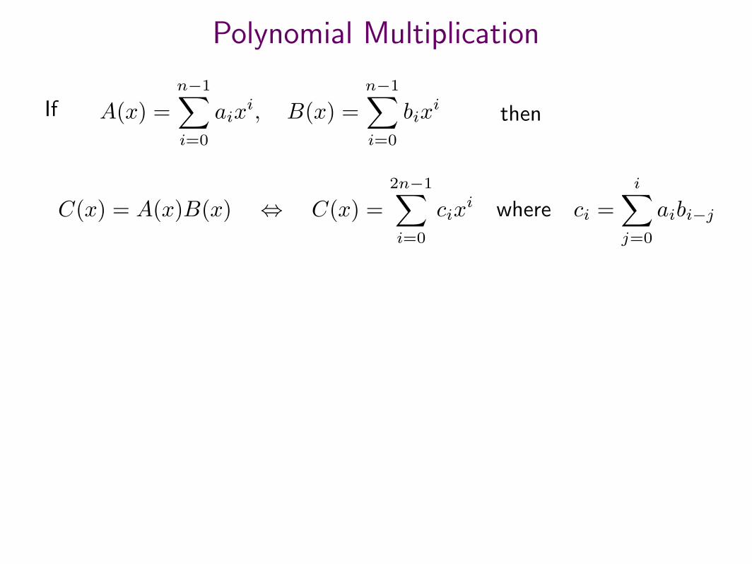
A(x) =n−1∑i=0
aixi, B(x) =
n−1∑i=0
bixiIf then
C(x) = A(x)B(x) ⇔ C(x) =2n−1∑i=0
cixi where ci =
i∑j=0
aibi−j
Polynomial Multiplication
A(x) =n−1∑i=0
aixi, B(x) =
n−1∑i=0
bixiIf then
C(x) = A(x)B(x) ⇔ C(x) =2n−1∑i=0
cixi where ci =
i∑j=0
aibi−j
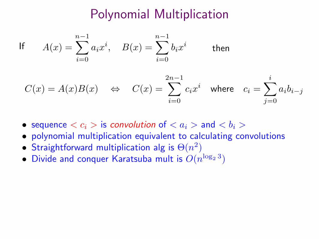
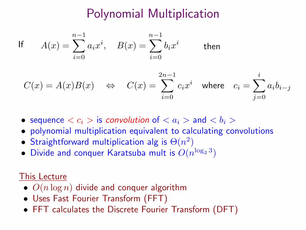
• sequence < ci > is convolution of < ai > and < bi >• polynomial multiplication equivalent to calculating convolutions• Straightforward multiplication alg is Θ(n2)• Divide and conquer Karatsuba mult is O(nlog2 3)
Polynomial Multiplication
A(x) =n−1∑i=0
aixi, B(x) =
n−1∑i=0
bixiIf then
C(x) = A(x)B(x) ⇔ C(x) =2n−1∑i=0
cixi where ci =
i∑j=0
aibi−j
• sequence < ci > is convolution of < ai > and < bi >• polynomial multiplication equivalent to calculating convolutions• Straightforward multiplication alg is Θ(n2)• Divide and conquer Karatsuba mult is O(nlog2 3)
This Lecture• O(n log n) divide and conquer algorithm• Uses Fast Fourier Transform (FFT)• FFT calculates the Discrete Fourier Transform (DFT)
Polynomial Evaluation & Interpolation
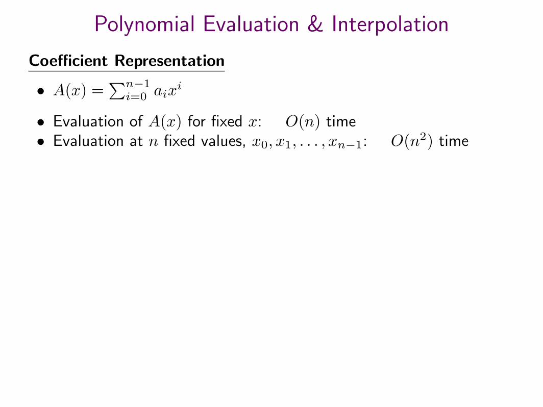
Coefficient Representation
• A(x) =∑n−1i=0 aix
i
• Evaluation of A(x) for fixed x: O(n) time• Evaluation at n fixed values, x0, x1, . . . , xn−1: O(n2) time
Polynomial Evaluation & Interpolation
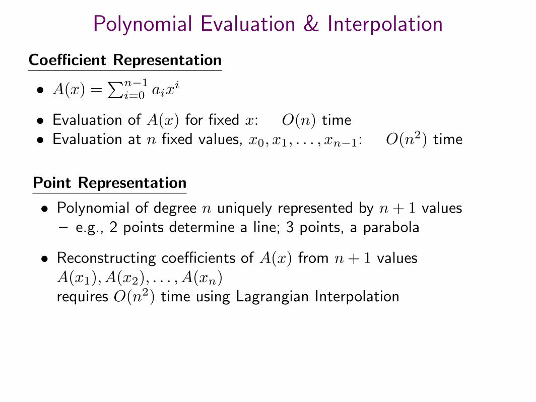
Coefficient Representation
• A(x) =∑n−1i=0 aix
i
• Evaluation of A(x) for fixed x: O(n) time• Evaluation at n fixed values, x0, x1, . . . , xn−1: O(n2) time
Point Representation
• Polynomial of degree n uniquely represented by n + 1 values– e.g., 2 points determine a line; 3 points, a parabola
• Reconstructing coefficients of A(x) from n + 1 valuesA(x1), A(x2), . . . , A(xn)requires O(n2) time using Lagrangian Interpolation
Review of Lagrangian Interpolation
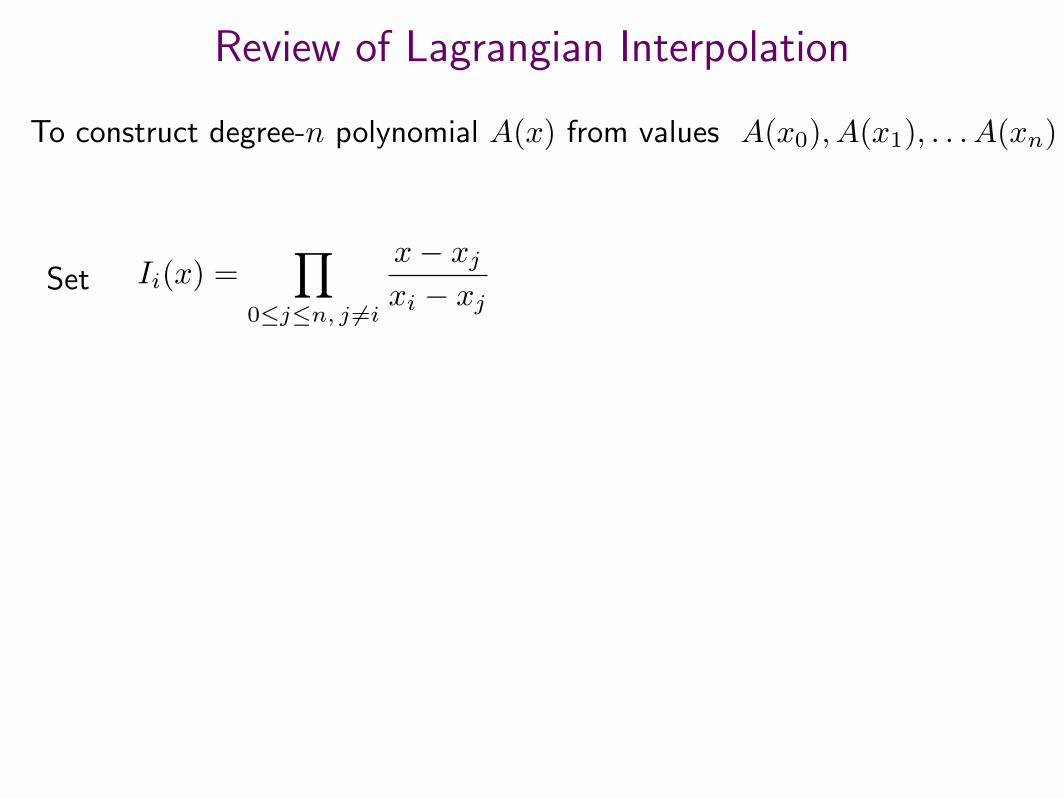
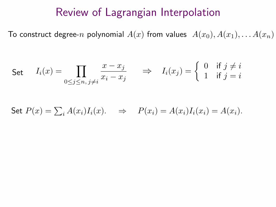
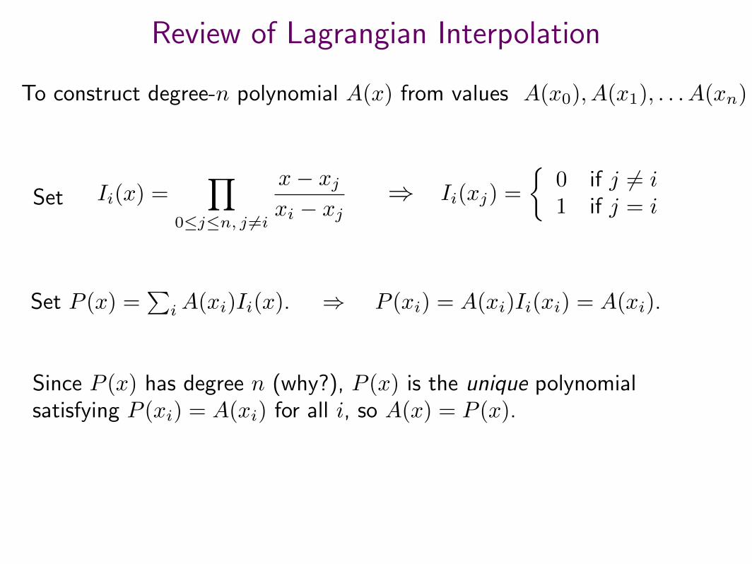
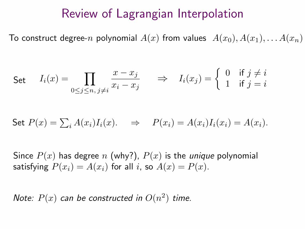
To construct degree-n polynomial A(x) from values A(x0), A(x1), . . . A(xn)
Ii(x) =∏
0≤j≤n, j 6=i
x− xjxi − xj
Set
Review of Lagrangian Interpolation
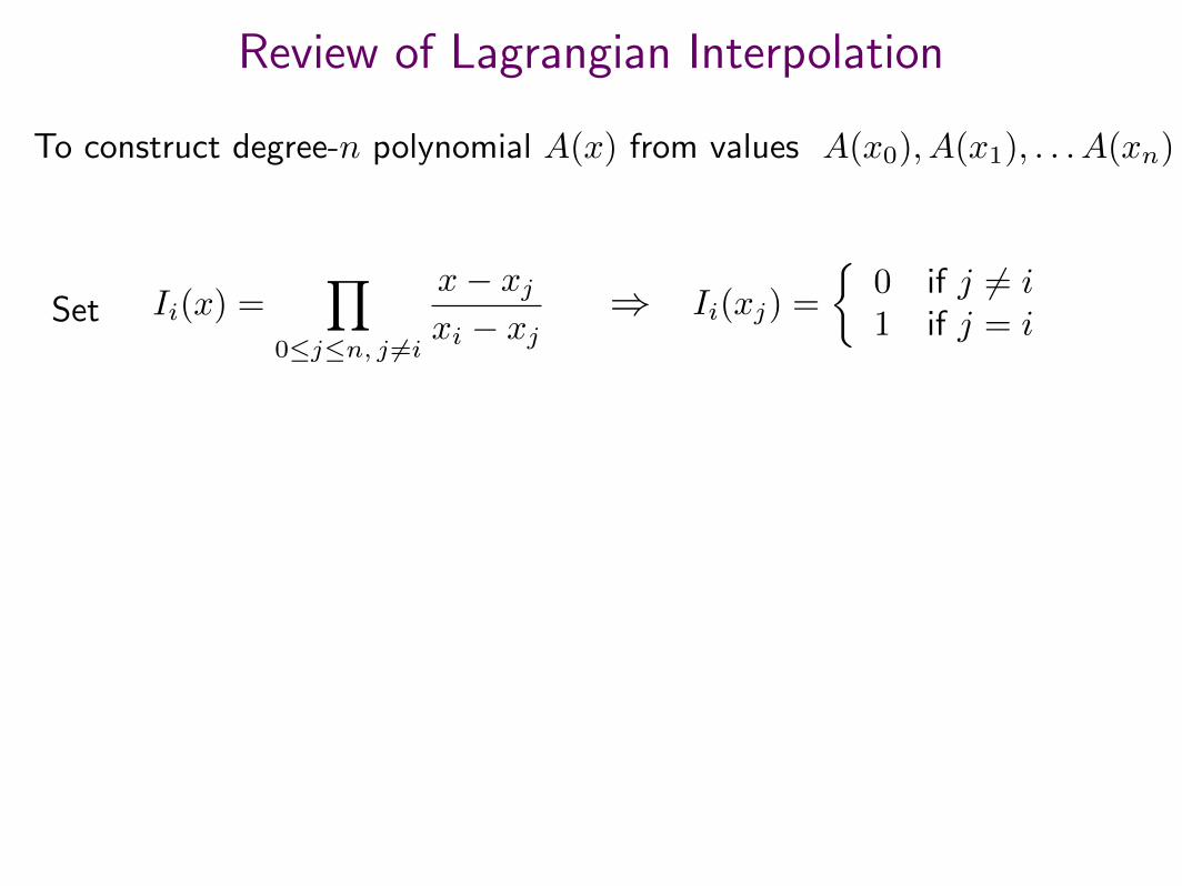
To construct degree-n polynomial A(x) from values A(x0), A(x1), . . . A(xn)
Ii(x) =∏
0≤j≤n, j 6=i
x− xjxi − xj
Set ⇒ Ii(xj) =
{0 if j 6= i1 if j = i
Review of Lagrangian Interpolation
To construct degree-n polynomial A(x) from values A(x0), A(x1), . . . A(xn)
Ii(x) =∏
0≤j≤n, j 6=i
x− xjxi − xj
Set ⇒ Ii(xj) =
{0 if j 6= i1 if j = i
Set P (x) =∑iA(xi)Ii(x). ⇒ P (xi) = A(xi)Ii(xi) = A(xi).
Review of Lagrangian Interpolation
To construct degree-n polynomial A(x) from values A(x0), A(x1), . . . A(xn)
Ii(x) =∏
0≤j≤n, j 6=i
x− xjxi − xj
Set ⇒ Ii(xj) =
{0 if j 6= i1 if j = i
Set P (x) =∑iA(xi)Ii(x). ⇒ P (xi) = A(xi)Ii(xi) = A(xi).
Since P (x) has degree n (why?), P (x) is the unique polynomialsatisfying P (xi) = A(xi) for all i, so A(x) = P (x).
Note: P (x) can be constructed in O(n2) time.
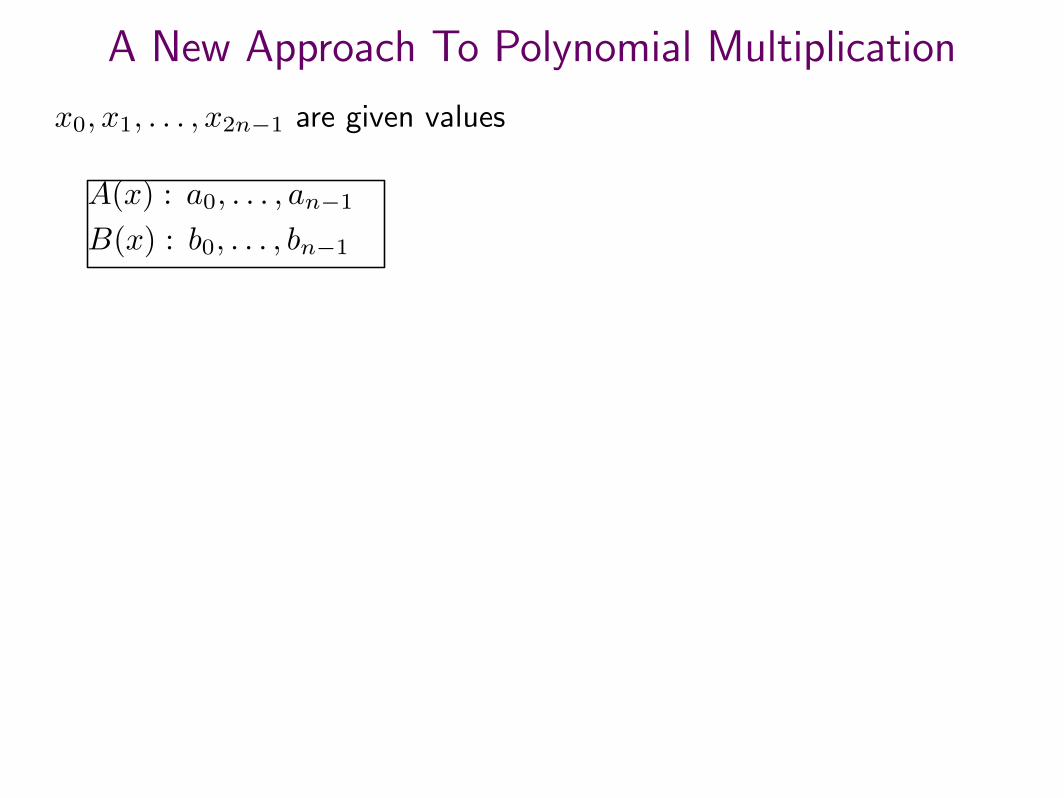
A New Approach To Polynomial Multiplication
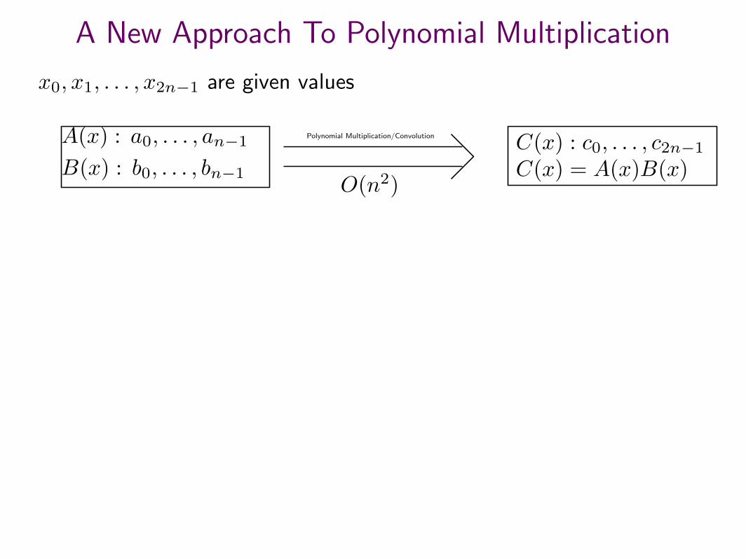
x0, x1, . . . , x2n−1 are given values
A(x) : a0, . . . , an−1
B(x) : b0, . . . , bn−1
A New Approach To Polynomial Multiplication
x0, x1, . . . , x2n−1 are given values
A(x) : a0, . . . , an−1
B(x) : b0, . . . , bn−1
C(x) : c0, . . . , c2n−1C(x) = A(x)B(x)
Polynomial Multiplication/Convolution
O(n2)
A New Approach To Polynomial Multiplication
x0, x1, . . . , x2n−1 are given values
A(x) : a0, . . . , an−1
B(x) : b0, . . . , bn−1
C(x) : c0, . . . , c2n−1C(x) = A(x)B(x)
Polynomial Multiplication/Convolution
O(n2)
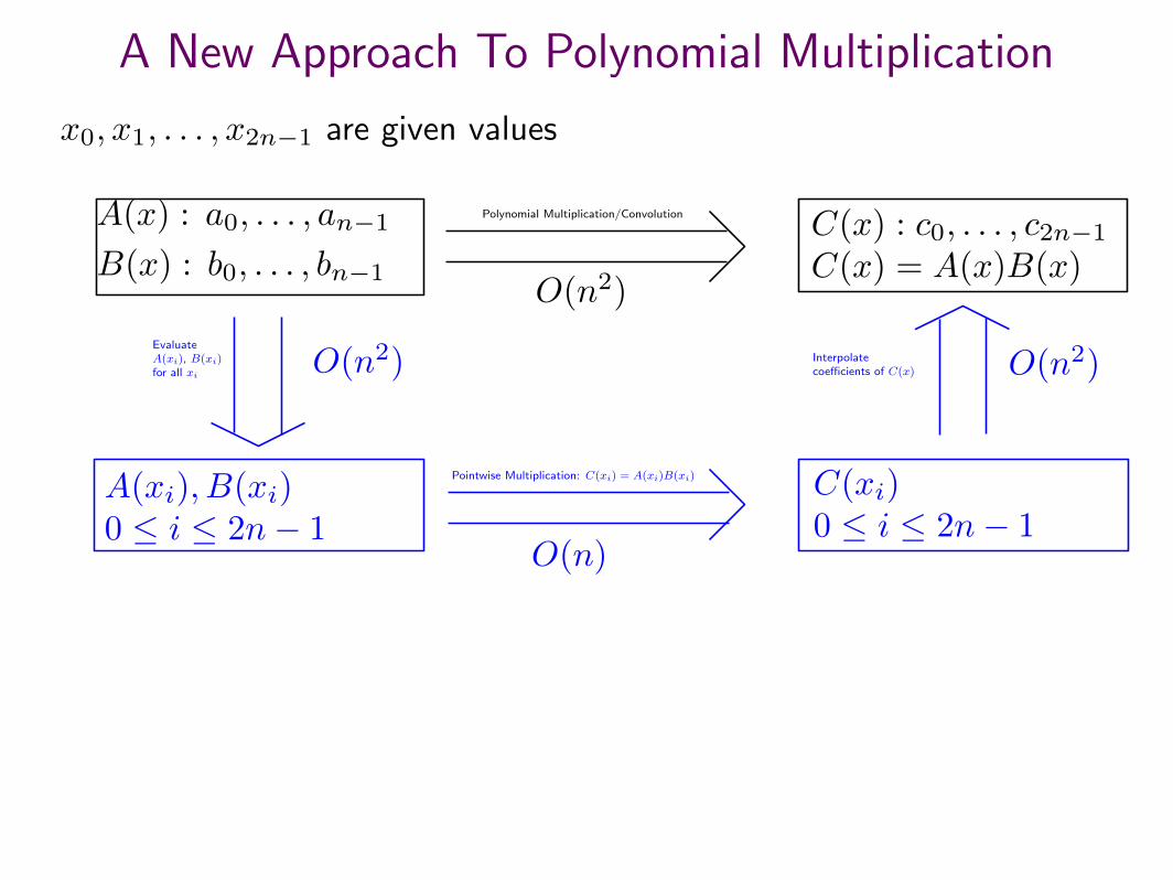
EvaluateA(xi), B(xi)for all xi
O(n2)
A(xi), B(xi)0 ≤ i ≤ 2n− 1
Pointwise Multiplication: C(xi) = A(xi)B(xi)
O(n)
C(xi)0 ≤ i ≤ 2n− 1
Interpolatecoefficients of C(x) O(n2)
A New Approach To Polynomial Multiplication
x0, x1, . . . , x2n−1 are given values
A(x) : a0, . . . , an−1
B(x) : b0, . . . , bn−1
C(x) : c0, . . . , c2n−1C(x) = A(x)B(x)
Polynomial Multiplication/Convolution
O(n2)
EvaluateA(xi), B(xi)for all xi
O(n2)
A(xi), B(xi)0 ≤ i ≤ 2n− 1
Pointwise Multiplication: C(xi) = A(xi)B(xi)
O(n)
C(xi)0 ≤ i ≤ 2n− 1
Interpolatecoefficients of C(x) O(n2)
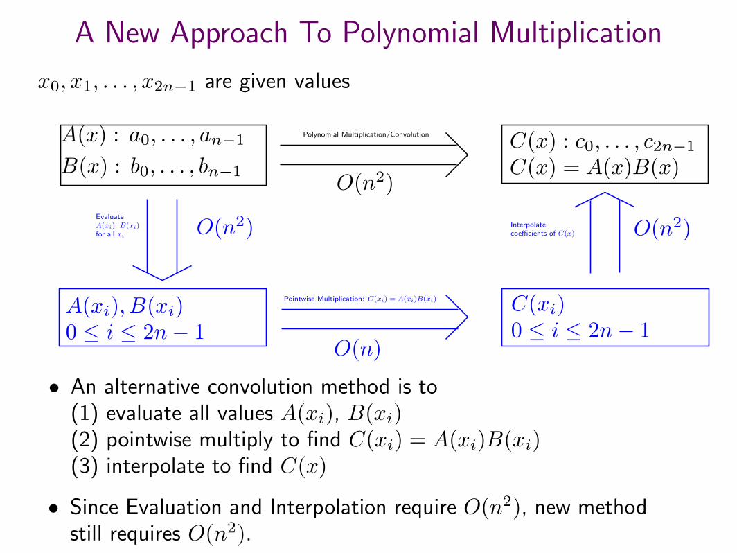
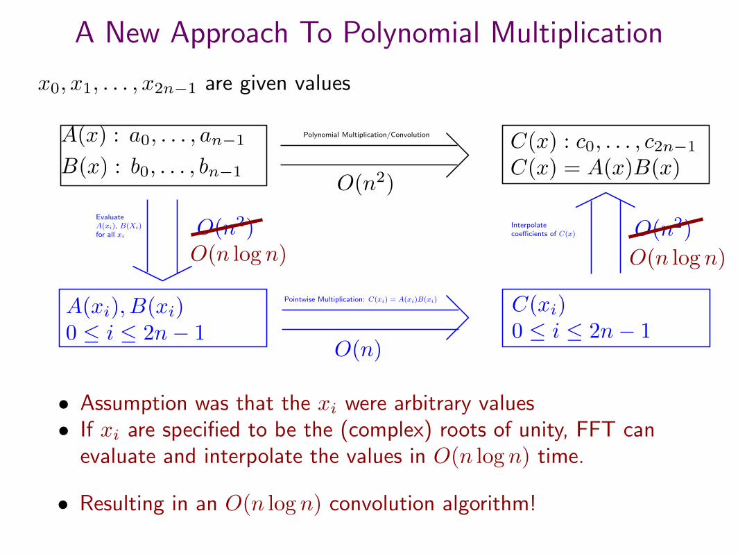
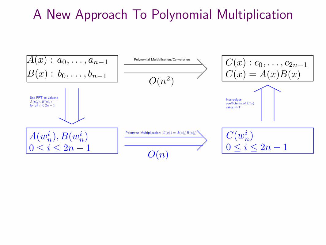
• An alternative convolution method is to(1) evaluate all values A(xi), B(xi)(2) pointwise multiply to find C(xi) = A(xi)B(xi)(3) interpolate to find C(x)
• Since Evaluation and Interpolation require O(n2), new methodstill requires O(n2).
A New Approach To Polynomial Multiplication
x0, x1, . . . , x2n−1 are given values
A(x) : a0, . . . , an−1
B(x) : b0, . . . , bn−1
C(x) : c0, . . . , c2n−1C(x) = A(x)B(x)
Polynomial Multiplication/Convolution
O(n2)
EvaluateA(xi), B(Xi)for all xi
O(n2)
A(xi), B(xi)0 ≤ i ≤ 2n− 1
Pointwise Multiplication: C(xi) = A(xi)B(xi)
O(n)
C(xi)0 ≤ i ≤ 2n− 1
Interpolatecoefficients of C(x) O(n2)
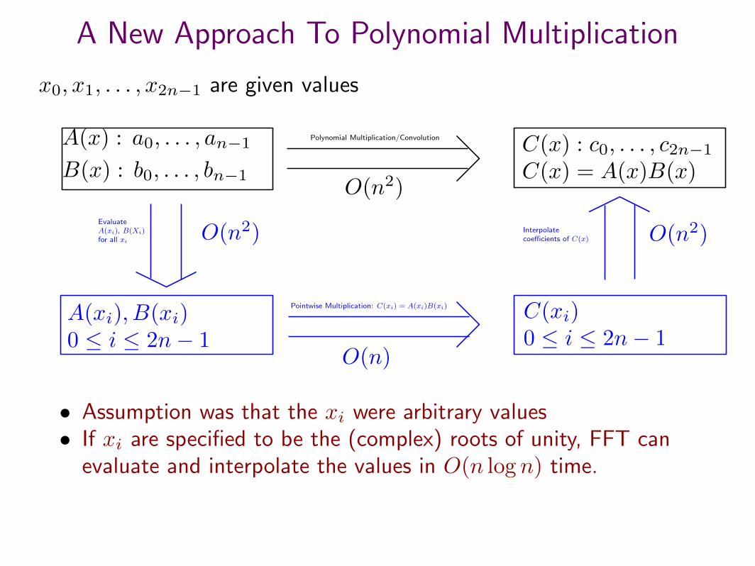
• Assumption was that the xi were arbitrary values• If xi are specified to be the (complex) roots of unity, FFT can
evaluate and interpolate the values in O(n log n) time.
A New Approach To Polynomial Multiplication
x0, x1, . . . , x2n−1 are given values
A(x) : a0, . . . , an−1
B(x) : b0, . . . , bn−1
C(x) : c0, . . . , c2n−1C(x) = A(x)B(x)
Polynomial Multiplication/Convolution
O(n2)
EvaluateA(xi), B(Xi)for all xi
O(n2)
A(xi), B(xi)0 ≤ i ≤ 2n− 1
Pointwise Multiplication: C(xi) = A(xi)B(xi)
O(n)
C(xi)0 ≤ i ≤ 2n− 1
Interpolatecoefficients of C(x) O(n2)
• Assumption was that the xi were arbitrary values• If xi are specified to be the (complex) roots of unity, FFT can
evaluate and interpolate the values in O(n log n) time.
• Resulting in an O(n log n) convolution algorithm!
O(n log n) O(n log n)
Review of Complex Numbers & Roots of Unity
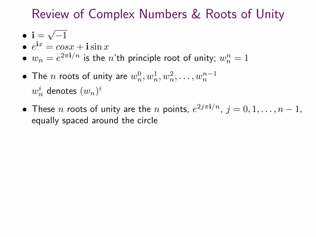
• i =√−1
• eix = cosx + i sinx• wn = e2πi/n is the n’th principle root of unity; wnn = 1
• The n roots of unity are w0n, w
1n, w
2n, . . . , w
n−1n
win denotes (wn)i
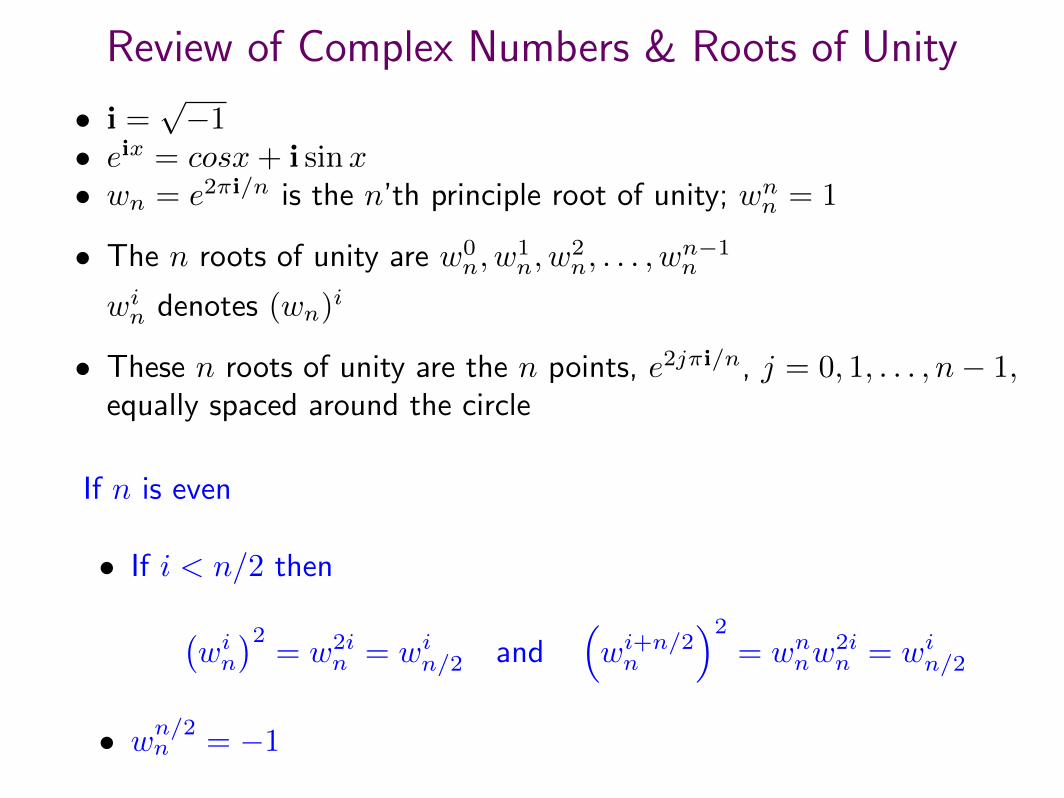
• These n roots of unity are the n points, e2jπi/n, j = 0, 1, . . . , n− 1,equally spaced around the circle
Review of Complex Numbers & Roots of Unity
• i =√−1
• eix = cosx + i sinx• wn = e2πi/n is the n’th principle root of unity; wnn = 1
• The n roots of unity are w0n, w
1n, w
2n, . . . , w
n−1n
win denotes (wn)i
• These n roots of unity are the n points, e2jπi/n, j = 0, 1, . . . , n− 1,equally spaced around the circle
If n is even
• If i < n/2 then
(win)2
= w2in = win/2 and
(wi+n/2n
)2= wnnw
2in = win/2
• wn/2n = −1
FFT Definition
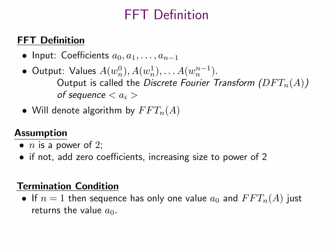
FFT Definition
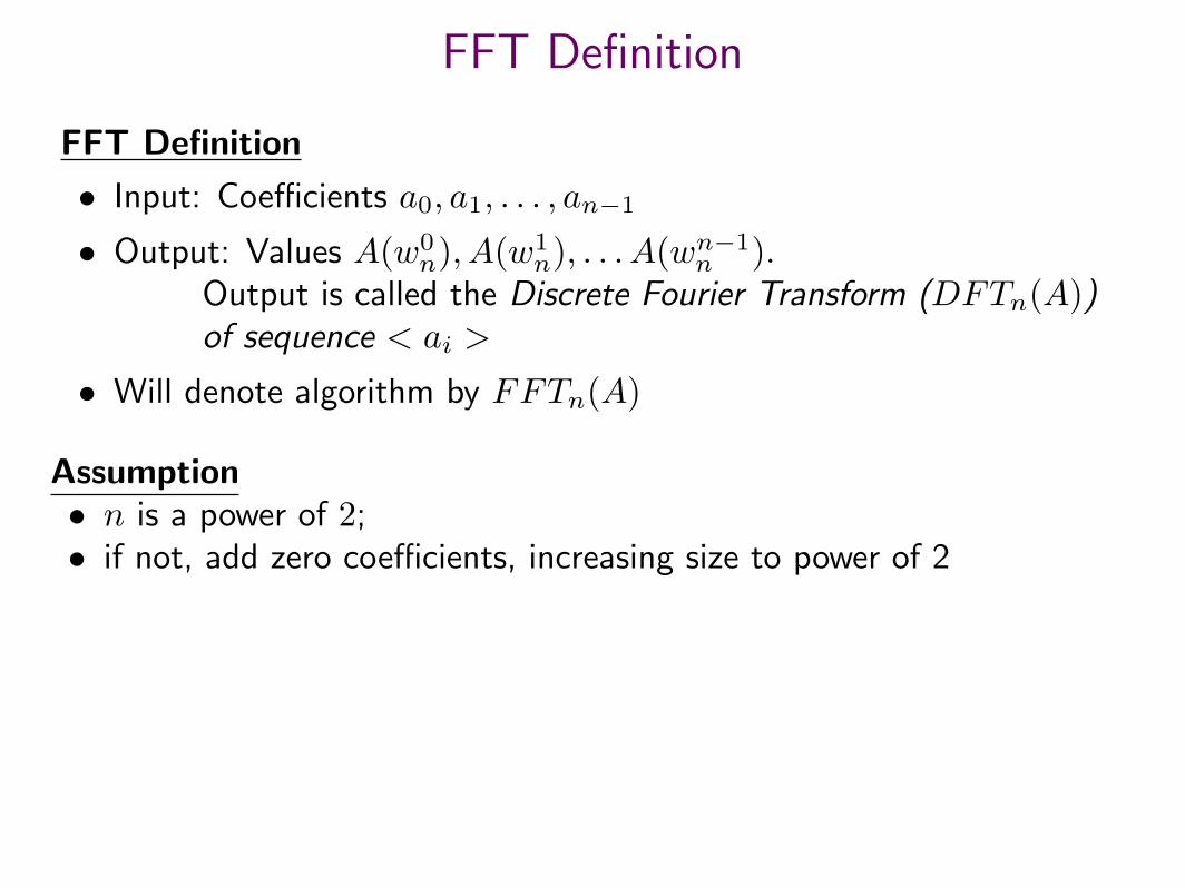
• Input: Coefficients a0, a1, . . . , an−1
• Output: Values A(w0n), A(w1
n), . . . A(wn−1n ).Output is called the Discrete Fourier Transform (DFTn(A))of sequence < ai >
• Will denote algorithm by FFTn(A)
Assumption• n is a power of 2;• if not, add zero coefficients, increasing size to power of 2
FFT Definition
FFT Definition
• Input: Coefficients a0, a1, . . . , an−1
• Output: Values A(w0n), A(w1
n), . . . A(wn−1n ).Output is called the Discrete Fourier Transform (DFTn(A))of sequence < ai >
• Will denote algorithm by FFTn(A)
Assumption• n is a power of 2;• if not, add zero coefficients, increasing size to power of 2
Termination Condition• If n = 1 then sequence has only one value a0 and FFTn(A) just
returns the value a0.
FFT Main Body
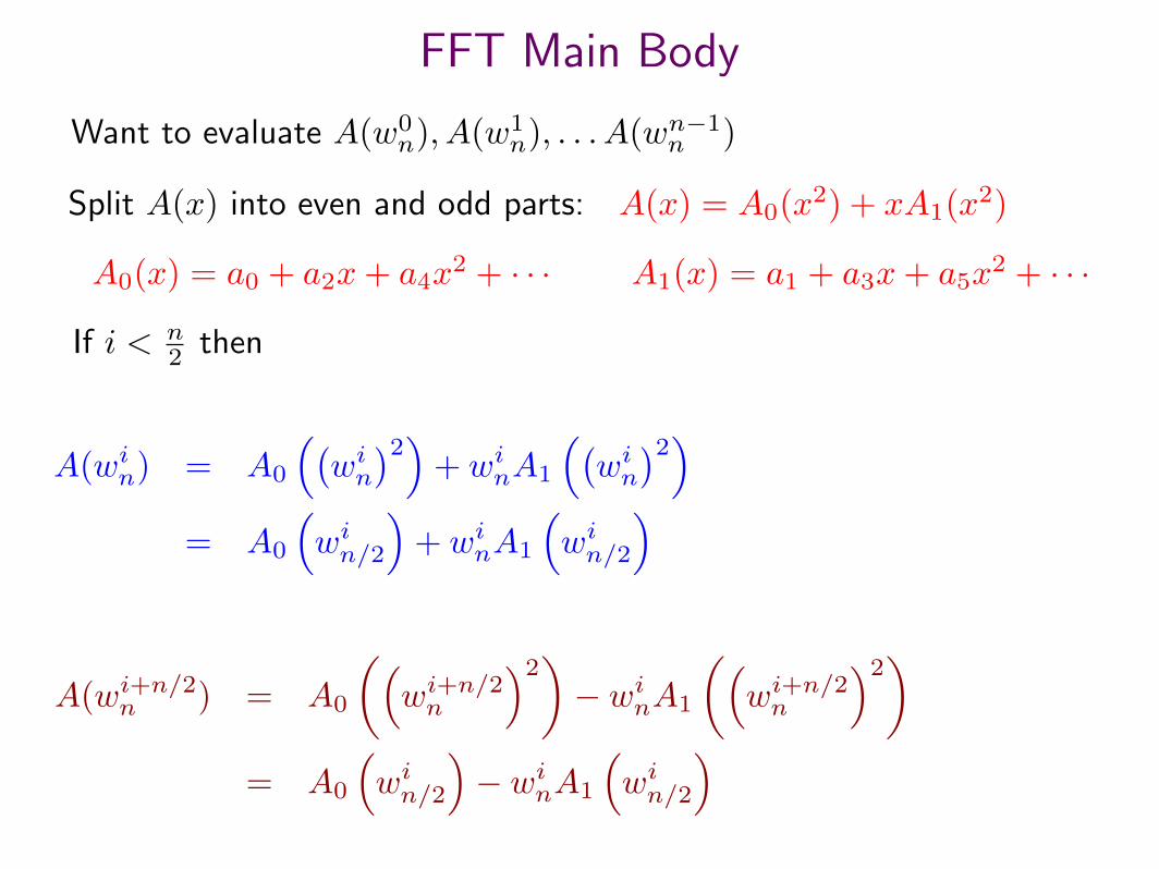
Want to evaluate A(w0n), A(w1
n), . . . A(wn−1n )
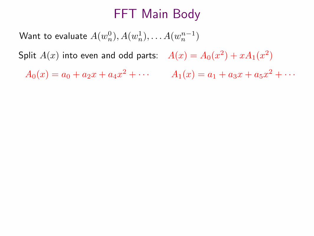
FFT Main Body
Want to evaluate A(w0n), A(w1
n), . . . A(wn−1n )
Split A(x) into even and odd parts: A(x) = A0(x2) + xA1(x2)
A0(x) = a0 + a2x + a4x2 + · · · A1(x) = a1 + a3x + a5x
2 + · · ·
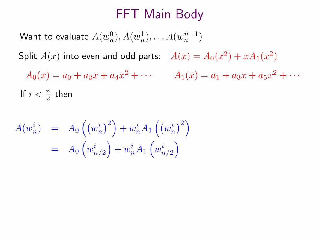
FFT Main Body
Want to evaluate A(w0n), A(w1
n), . . . A(wn−1n )
Split A(x) into even and odd parts: A(x) = A0(x2) + xA1(x2)
A0(x) = a0 + a2x + a4x2 + · · · A1(x) = a1 + a3x + a5x
2 + · · ·
If i < n2 then
A(win) = A0
((win)2)
+ winA1
((win)2)
= A0
(win/2
)+ winA1
(win/2
)
FFT Main Body
Want to evaluate A(w0n), A(w1
n), . . . A(wn−1n )
Split A(x) into even and odd parts: A(x) = A0(x2) + xA1(x2)
A0(x) = a0 + a2x + a4x2 + · · · A1(x) = a1 + a3x + a5x
2 + · · ·
If i < n2 then
A(win) = A0
((win)2)
+ winA1
((win)2)
= A0
(win/2
)+ winA1
(win/2
)
A(wi+n/2n ) = A0
((wi+n/2n
)2)− winA1
((wi+n/2n
)2)= A0
(win/2
)− winA1
(win/2
)
FFT Algorithm
A(win) = A0
(win/2
)+ winA1
(win/2
)A(wi+n/2n ) = A0
(win/2
)− winA1
(win/2
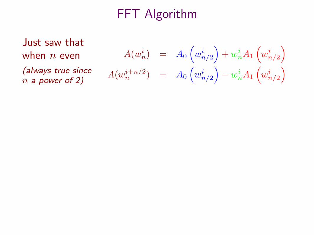
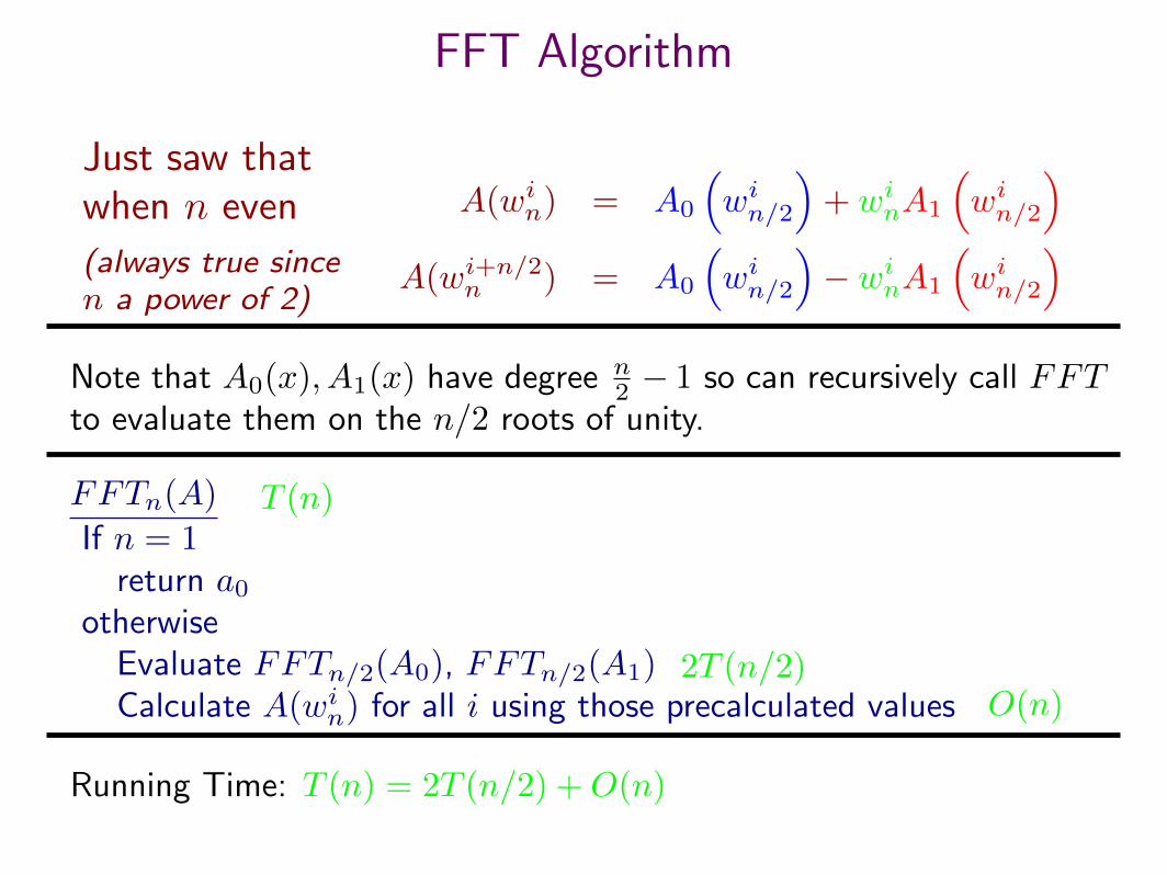
)Just saw thatwhen n even
(always true sincen a power of 2)
FFT Algorithm
A(win) = A0
(win/2
)+ winA1
(win/2
)A(wi+n/2n ) = A0
(win/2
)− winA1
(win/2
)Just saw thatwhen n even
(always true sincen a power of 2)
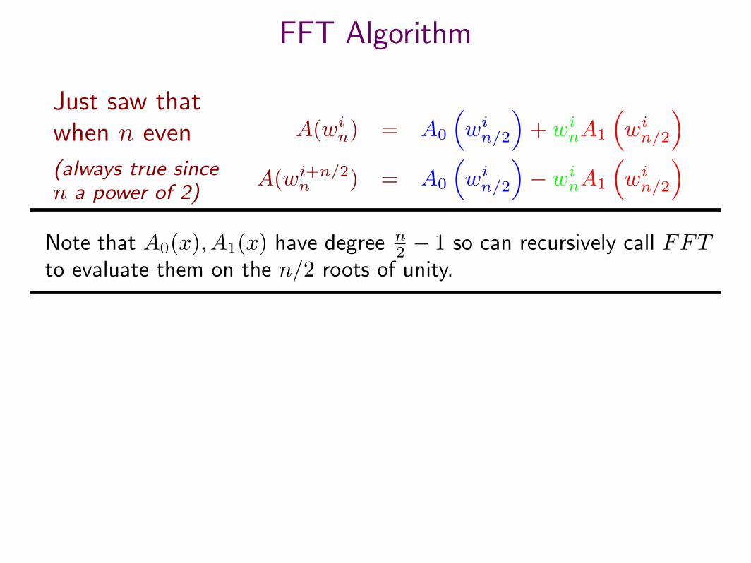
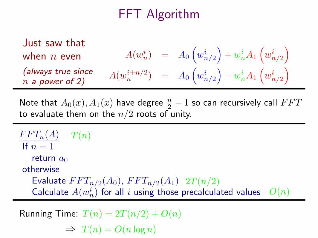
Note that A0(x), A1(x) have degree n2 − 1 so can recursively call FFT
to evaluate them on the n/2 roots of unity.
FFT Algorithm
A(win) = A0
(win/2
)+ winA1
(win/2
)A(wi+n/2n ) = A0
(win/2
)− winA1
(win/2
)Just saw thatwhen n even
(always true sincen a power of 2)
Note that A0(x), A1(x) have degree n2 − 1 so can recursively call FFT
to evaluate them on the n/2 roots of unity.
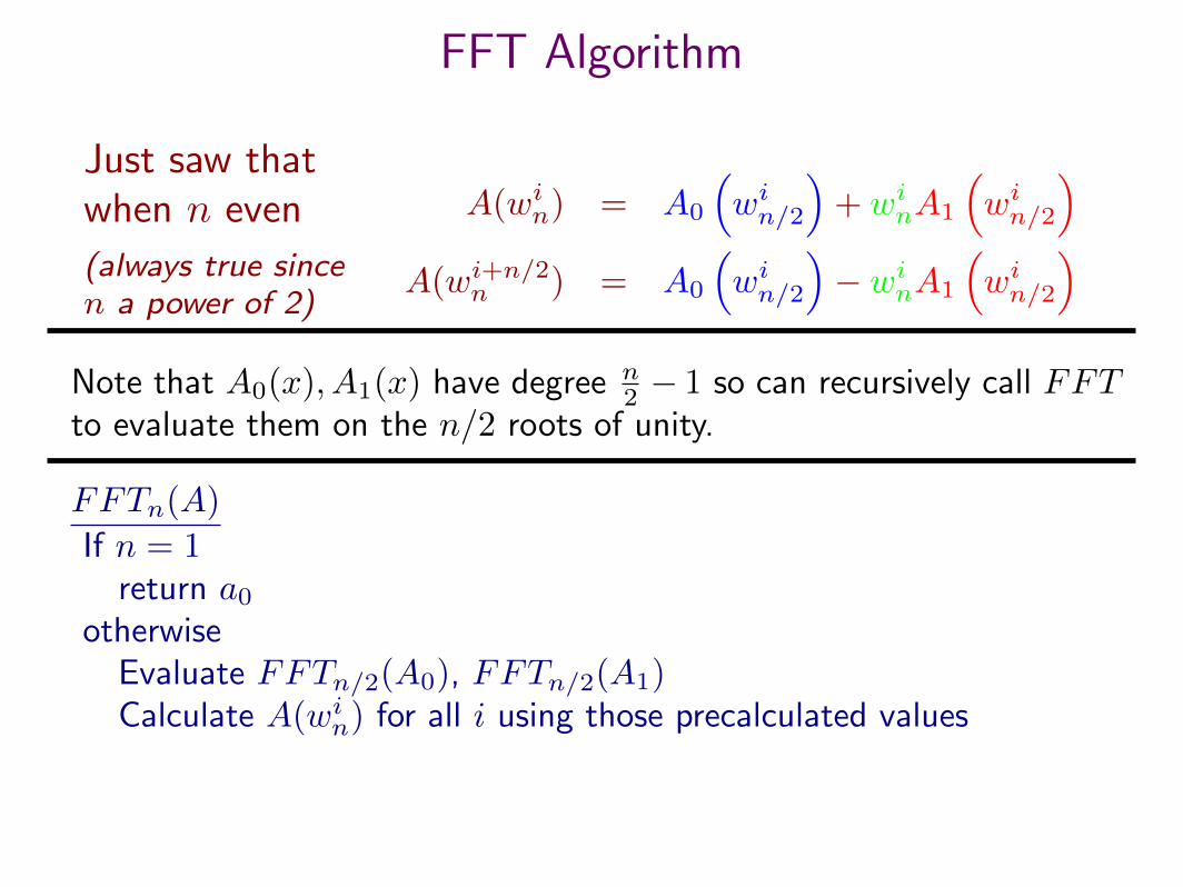
FFTn(A)
If n = 1return a0
otherwiseEvaluate FFTn/2(A0), FFTn/2(A1)Calculate A(win) for all i using those precalculated values
FFT Algorithm
A(win) = A0
(win/2
)+ winA1
(win/2
)A(wi+n/2n ) = A0
(win/2
)− winA1
(win/2
)Just saw thatwhen n even
(always true sincen a power of 2)
Note that A0(x), A1(x) have degree n2 − 1 so can recursively call FFT
to evaluate them on the n/2 roots of unity.
FFTn(A)
If n = 1return a0
otherwiseEvaluate FFTn/2(A0), FFTn/2(A1)Calculate A(win) for all i using those precalculated values
Running Time: T (n) = 2T (n/2) + O(n)
T (n)
2T (n/2)O(n)
⇒ T (n) = O(n log n)
FFT Based Interpolation
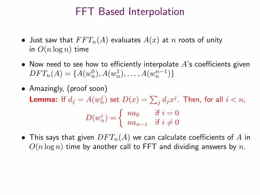
• Just saw that FFTn(A) evaluates A(x) at n roots of unityin O(n log n) time
• Now need to see how to efficiently interpolate A’s coefficients givenDFTn(A) = {A(w0
n), A(w1n), . . . , A(wn−1n )}
• Amazingly, (proof soon)
Lemma: If dj = A(wjn) set D(x) =∑j djx
j . Then, for all i < n,
D(win) =
{na0 if i = 0nan−i if i 6= 0
• This says that given DFTn(A) we can calculate coefficients of A inO(n log n) time by another call to FFT and dividing answers by n.
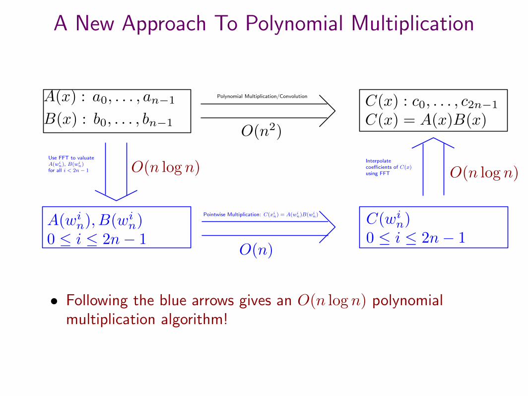
A New Approach To Polynomial Multiplication
A(x) : a0, . . . , an−1
B(x) : b0, . . . , bn−1
C(x) : c0, . . . , c2n−1C(x) = A(x)B(x)
Polynomial Multiplication/Convolution
O(n2)
Use FFT to valuateA(wi
n), B(win)
for all i < 2n− 1
A(win), B(win)0 ≤ i ≤ 2n− 1
Pointwise Multiplication: C(xin) = A(wi
n)B(win)
O(n)
C(win)0 ≤ i ≤ 2n− 1
Interpolatecoefficients of C(x)using FFT
• Following the blue arrows gives an O(n log n) polynomialmultiplication algorithm!
O(n log n) O(n log n)
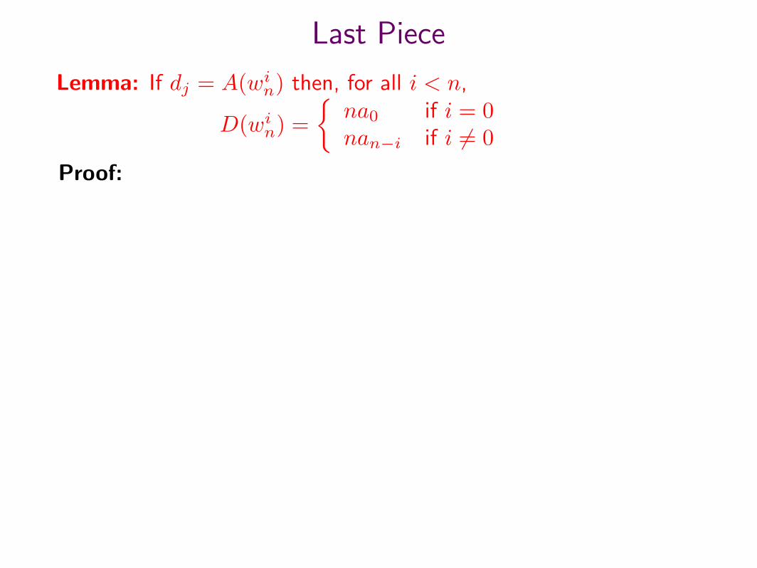
Last Piece
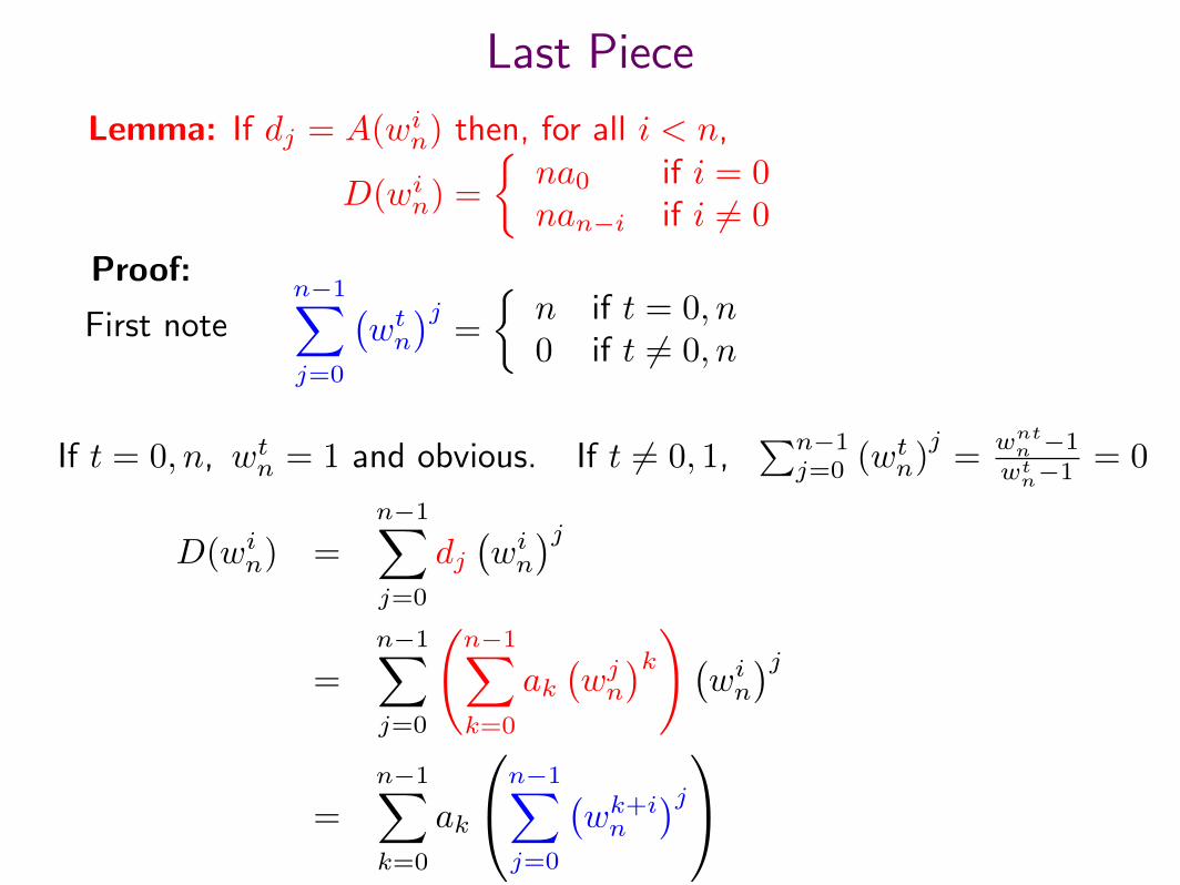
Lemma: If dj = A(win) then, for all i < n,
D(win) =
{na0 if i = 0nan−i if i 6= 0
Proof:
Last Piece
Lemma: If dj = A(win) then, for all i < n,
D(win) =
{na0 if i = 0nan−i if i 6= 0
Proof:
First noten−1∑j=0
(wtn)j
=
{n if t = 0, n0 if t 6= 0, n
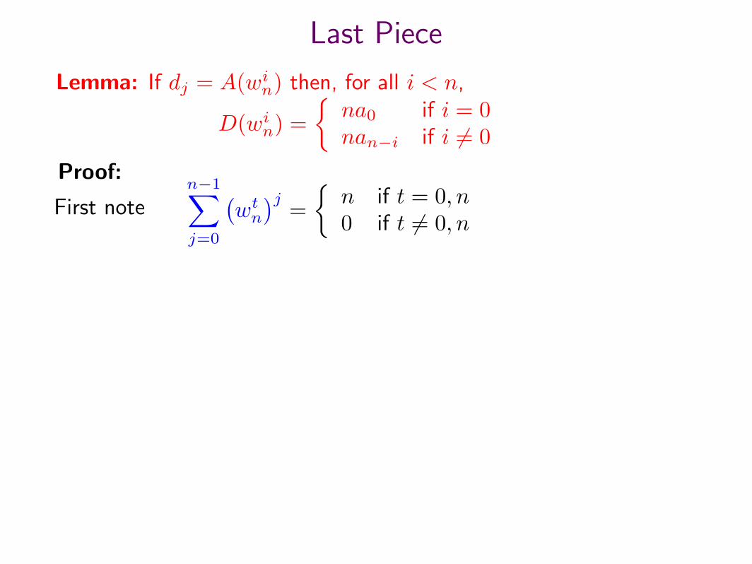
Last Piece
Lemma: If dj = A(win) then, for all i < n,
D(win) =
{na0 if i = 0nan−i if i 6= 0
Proof:
First noten−1∑j=0
(wtn)j
=
{n if t = 0, n0 if t 6= 0, n
If t = 0, n, wtn = 1 and obvious. If t 6= 0, 1,∑n−1j=0 (wtn)
j=
wntn −1wt
n−1= 0
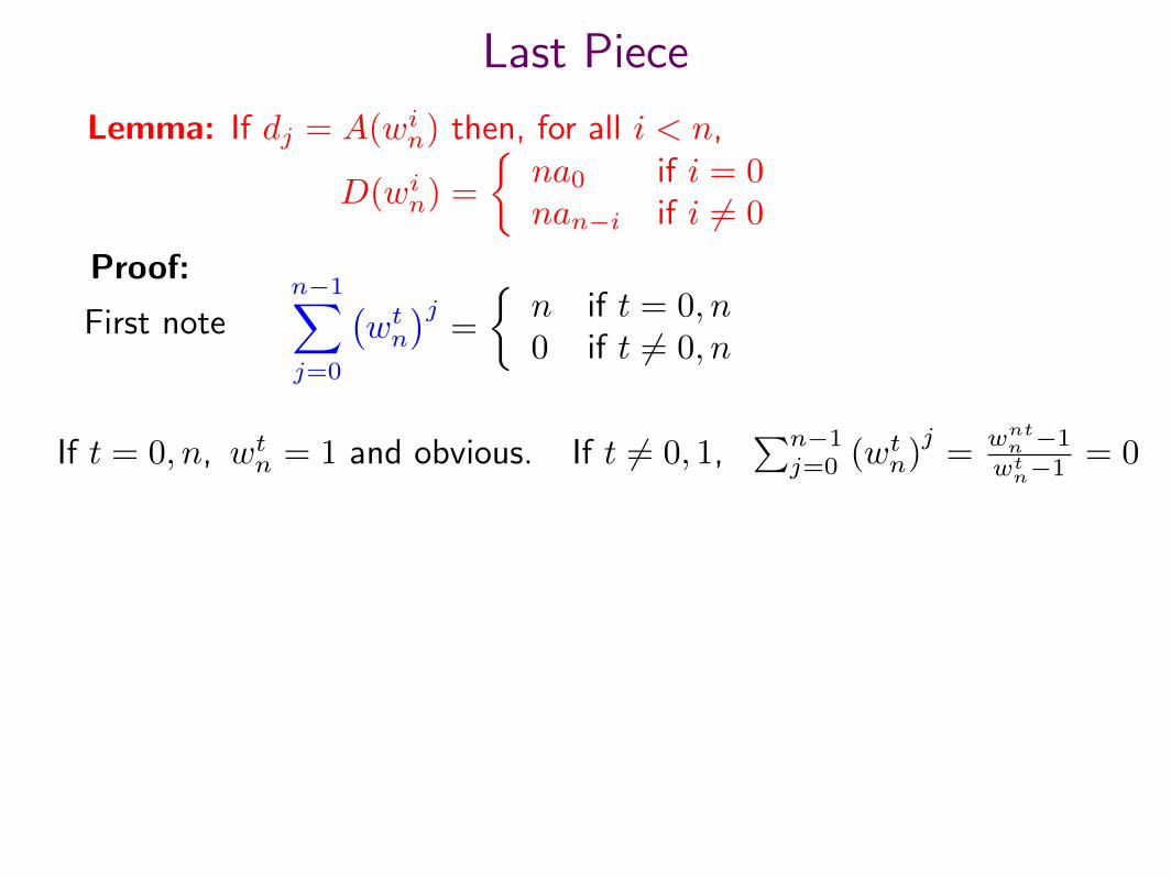
Last Piece
Lemma: If dj = A(win) then, for all i < n,
D(win) =
{na0 if i = 0nan−i if i 6= 0
Proof:
First noten−1∑j=0
(wtn)j
=
{n if t = 0, n0 if t 6= 0, n
If t = 0, n, wtn = 1 and obvious. If t 6= 0, 1,∑n−1j=0 (wtn)
j=
wntn −1wt
n−1= 0
D(win) =
n−1∑j=0
dj(win)j
=n−1∑j=0
(n−1∑k=0
ak(wjn)k)(
win)j
=
n−1∑k=0
ak
n−1∑j=0
(wk+in
)j
Last Piece
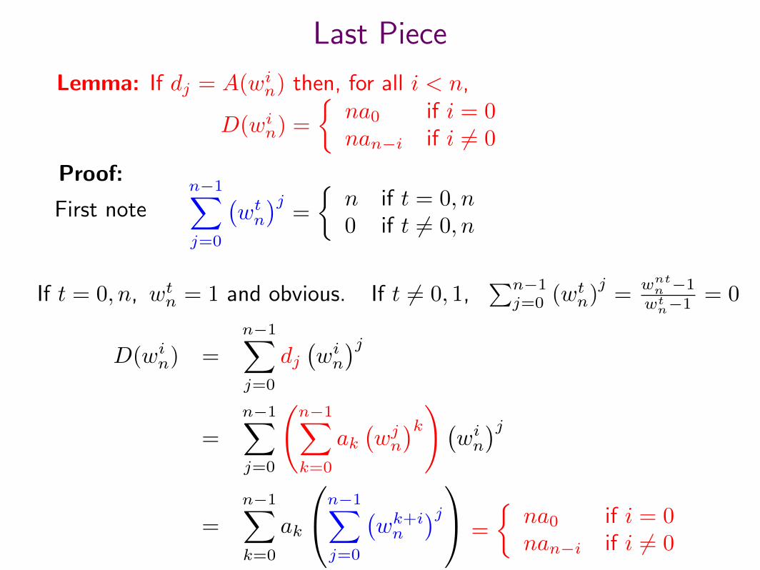
Lemma: If dj = A(win) then, for all i < n,
D(win) =
{na0 if i = 0nan−i if i 6= 0
Proof:
First noten−1∑j=0
(wtn)j
=
{n if t = 0, n0 if t 6= 0, n
If t = 0, n, wtn = 1 and obvious. If t 6= 0, 1,∑n−1j=0 (wtn)
j=
wntn −1wt
n−1= 0
D(win) =
n−1∑j=0
dj(win)j
=n−1∑j=0
(n−1∑k=0
ak(wjn)k)(
win)j
=
n−1∑k=0
ak
n−1∑j=0
(wk+in
)j =
{na0 if i = 0nan−i if i 6= 0
Odds and Ends
• Note that FFT presented here as divide-and-conquer algorithm
• Can also be written iteratively and also implemented in adedicated circuit (butterfly pattern)
• Can design O(n log n) algorithms that work on powers of othernumbers, e.g., n = 3k or n = 5k.
• Some other transforms using other orthogonal function basescan be implemented quickly, similar to the FFT, e.g.,Hadamard Transforms
• Gauss actually developed something similar to FFT in 1805.Rediscovered many times afterwards
• Was “forgotten” until Cooley and Tukey published a paperdescribing it in 1965.After that, became one of the most used algorithms in theworld!
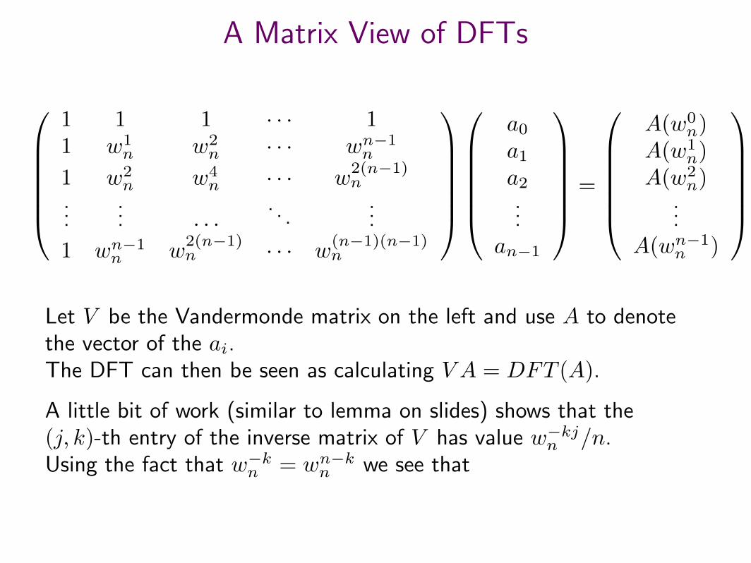
A Matrix View of DFTs
1 1 1 · · · 11 w1
n w2n · · · wn−1n
1 w2n w4
n · · · w2(n−1)n
...... . . .
. . ....
1 wn−1n w2(n−1)n · · · w
(n−1)(n−1)n
a0a1a2...
an−1
=
A(w0
n)A(w1
n)A(w2
n)...
A(wn−1n )
Let V be the Vandermonde matrix on the left and use A to denotethe vector of the ai.The DFT can then be seen as calculating V A = DFT (A).
A little bit of work (similar to lemma on slides) shows that the(j, k)-th entry of the inverse matrix of V has value w−kjn /n.Using the fact that w−kn = wn−kn we see that
V =
1 1 1 · · · 1
1 w1n w2
n · · · wn−1n
1 w2n w4
n · · · w2(n−1)n
...... . . .
. . ....
1 wn−1n w
2(n−1)n · · · w
(n−1)(n−1)n
and V −1 =1
n
1 1 1 · · · 1
1 wn−1n w
2(n−1)n · · · w
(n−1)(n−1)n
1 wn−2n w
2(n−2)n · · · w
(n−1)(n−2)n
...... . . .
. . ....
1 w1n w2
n · · · wn−1n
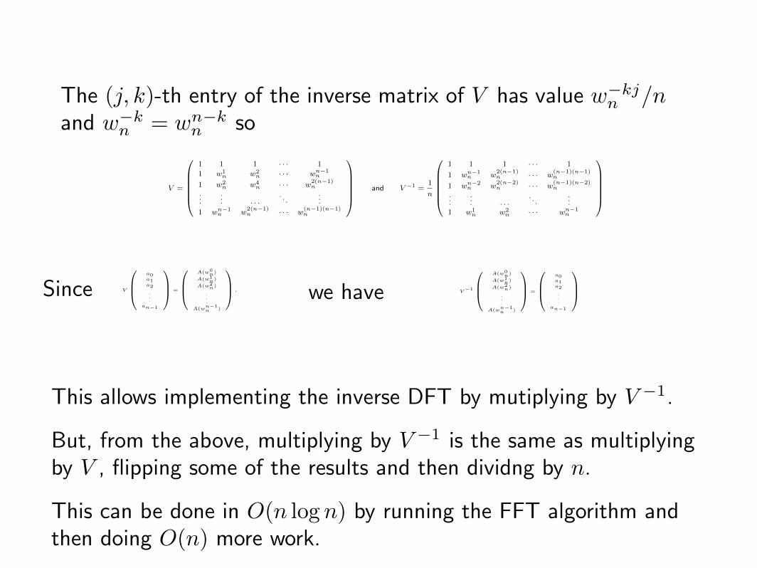
The (j, k)-th entry of the inverse matrix of V has value w−kjn /nand w−kn = wn−kn so
V
a0a1a2
.
.
.an−1
=
A(w0
n)
A(w1n)
A(w2n)
.
.
.
A(wn−1n )
,Since we have V−1
A(w0
n)
A(w1n)
A(w2n)
.
.
.
A(wn−1n )
=
a0a1a2
.
.
.an−1
This allows implementing the inverse DFT by mutiplying by V −1.
But, from the above, multiplying by V −1 is the same as multiplyingby V , flipping some of the results and then dividng by n.
This can be done in O(n log n) by running the FFT algorithm andthen doing O(n) more work.
1 x1 x2
1 · · · xn−11
1 x2 x22 · · · xn−12
1 x3 x23 · · · xn−13
...... . . .
. . ....
1 xn x2n · · · xn−1n
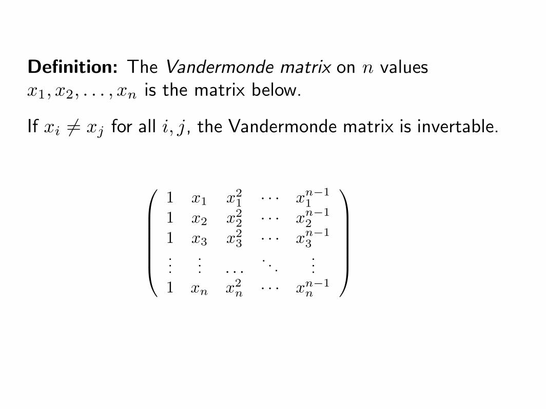
Definition: The Vandermonde matrix on n valuesx1, x2, . . . , xn is the matrix below.
If xi 6= xj for all i, j, the Vandermonde matrix is invertable.


![Practical Fast Polynomial Multiplication - Computer …moreno/CS424/Ressources/RobertTMoenck.Practica… · Multiplication 0(N log N) [Pol 71] Division with Remainder 0(N log N) [Str](https://img.pdfslide.us/doc/110x75/5aa47bf87f8b9ac8748c0012/practical-fast-polynomial-multiplication-computer-morenocs424ressources.jpg)