Robot Design

Optimization

by means of a

Genetic Algorithm and

Physics Simulation

Morgan Gunnarsson

December 2, 2010

Master’s Thesis in Computing Science, 30 ECTS credits

Supervisor at CS-UmU: Thomas Hellström

Examiner: Per Lindström

Umeå University

Department of Computing Science

SE-901 87 UMEÅ

SWEDEN

Abstract

This thesis presents a new robot design paradigm that utilizes evolutionary optimization

techniques and advanced physics simulations. This technology makes it possible to design and

test robots in virtual environments before the physical robots are built, which enables robot

manufacturers to improve the performance of their products and decrease the time and cost

for development. In this project, a 3D robot model was defined in geometric, kinematic and

dynamic terms. Also, a piece of software was developed in C++ to optimize the robot design,

and to simulate and visualize the robot model with the aid of a physics engine. A genetic

algorithm was developed for the optimization and used to minimize the average positional

error and the total torque magnitude under constraints on speed, and the design variables

were the PID controller parameters and the torque actuator limits. Only predefined robots can

be programmed and simulated with current software packages for offline-programming and

robot simulation. It was concluded that such software packages can be improved by robot

design optimization using the software developed in this project, by means of a genetic

algorithm and simulations using a physics engine.

ii

iii

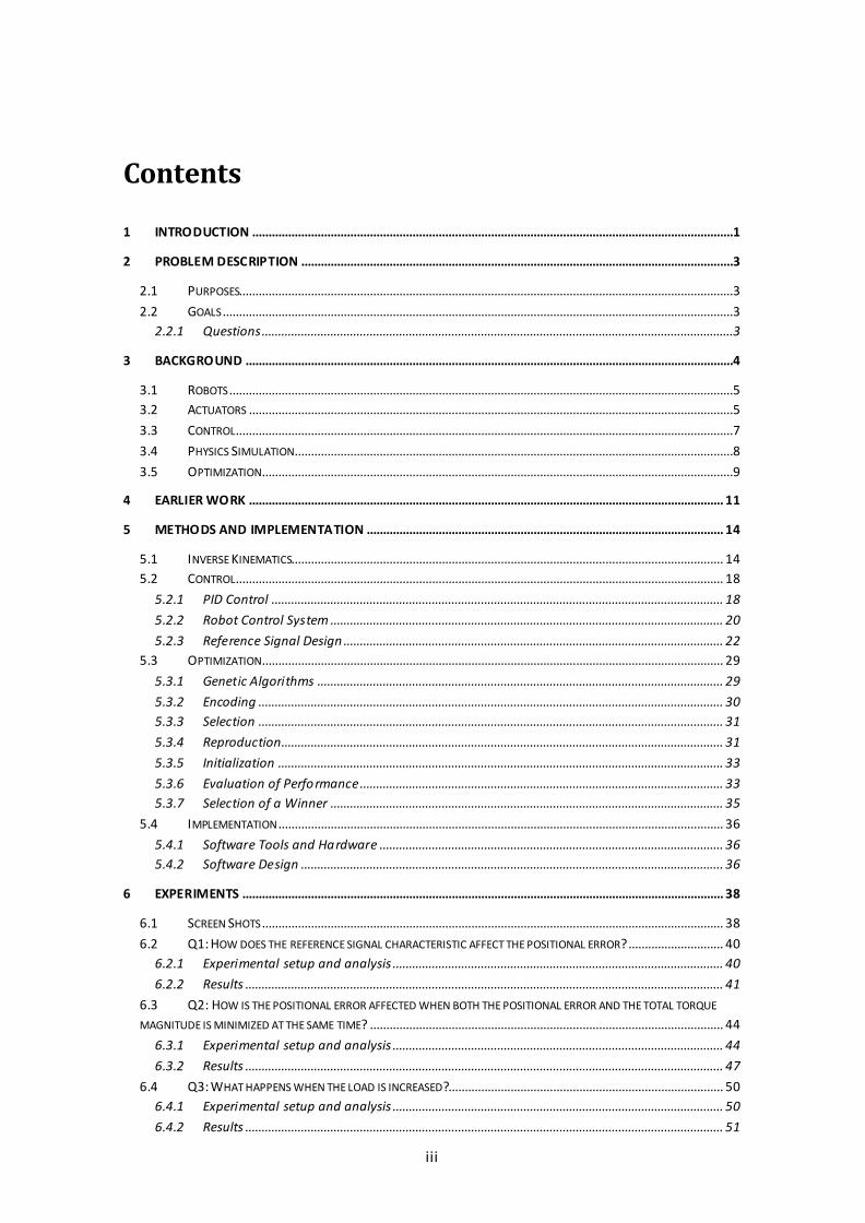
Contents

1 INTRODUCTION ...................................................................................................................................................1

2 PROBLEM DESCRIPTION ....................................................................................................................................3

2.1 PURPOSES.......................................................................................................................................................3

2.2 GOALS ............................................................................................................................................................3 2.2.1 Questions................................................................................................................................................3

3 BACKGROUND .....................................................................................................................................................4

3.1 ROBOTS ..........................................................................................................................................................5 3.2 ACTUATORS ....................................................................................................................................................5

3.3 CONTROL........................................................................................................................................................7

3.4 PHYSICS SIMULATION ......................................................................................................................................8

3.5 OPTIMIZATION ................................................................................................................................................9

4 EARLIER WORK ................................................................................................................................................. 11

5 METHODS AND IMPLEMENTATION ............................................................................................................. 14

5.1 INVERSE KINEMATICS.................................................................................................................................... 14 5.2 CONTROL..................................................................................................................................................... 18

5.2.1 PID Control .......................................................................................................................................... 18

5.2.2 Robot Control System ........................................................................................................................ 20

5.2.3 Reference Signal Design .................................................................................................................... 22 5.3 OPTIMIZATION ............................................................................................................................................. 29

5.3.1 Genetic Algorithms ............................................................................................................................ 29

5.3.2 Encoding .............................................................................................................................................. 30 5.3.3 Selection .............................................................................................................................................. 31

5.3.4 Reproduction....................................................................................................................................... 31

5.3.5 Initialization ........................................................................................................................................ 33

5.3.6 Evaluation of Performance............................................................................................................... 33 5.3.7 Selection of a Winner ........................................................................................................................ 35

5.4 IMPLEMENTATION ........................................................................................................................................ 36

5.4.1 Software Tools and Hardware ......................................................................................................... 36 5.4.2 Software Design ................................................................................................................................. 36

6 EXPERIMENTS ................................................................................................................................................... 38

6.1 SCREEN SHOTS ............................................................................................................................................. 38

6.2 Q1: HOW DOES THE REFERENCE SIGNAL CHARACTERISTIC AFFECT THE POSITIONAL ERROR? ............................. 40 6.2.1 Experimental setup and analysis ..................................................................................................... 40

6.2.2 Results .................................................................................................................................................. 41

6.3 Q2: HOW IS THE POSITIONAL ERROR AFFECTED WHEN BOTH THE POSITIONAL ERROR AND THE TOTAL TORQUE

MAGNITUDE IS MINIMIZED AT THE SAME TIME? ............................................................................................................ 44

6.3.1 Experimental setup and analysis ..................................................................................................... 44

6.3.2 Results .................................................................................................................................................. 47

6.4 Q3: WHAT HAPPENS WHEN THE LOAD IS INCREASED?.................................................................................... 50 6.4.1 Experimental setup and analysis ..................................................................................................... 50

6.4.2 Results .................................................................................................................................................. 51

iv

6.5 Q4: HOW IS THE POSITIONAL ERROR AFFECTED WHEN THE NOMINAL AVERAGE SPEED IS CHANGED? ................ 51

6.5.1 Experimental setup and analysis ..................................................................................................... 51

6.5.2 Results .................................................................................................................................................. 52

7 CONCLUSIONS................................................................................................................................................... 53

7.1 RESTRICTIONS AND LIMITATIONS ................................................................................................................... 53

7.2 FUTURE WORK ............................................................................................................................................. 54

8 ACKNOWLEDGEMENTS................................................................................................................................... 55

REFERENCES ................................................................................................................................................................ 56

APPENDIX A ................................................................................................................................................................ 58

EXPERIMENTAL SETUP PARAMETERS ............................................................................................................................ 58

Base controllers and actuators ....................................................................................................................... 58 Initial experiments ............................................................................................................................................ 58

Parameters in Q1 .............................................................................................................................................. 59

Physics Engine Parameters ............................................................................................................................. 60 RESULT DATA ............................................................................................................................................................. 60

Optimized design variables in Q1 .................................................................................................................. 60

Optimized design variables in Q2 .................................................................................................................. 62

Optimized design variables in Q3 .................................................................................................................. 62

APPENDIX B................................................................................................................................................................. 63

ROBOT CAD DRAWING............................................................................................................................................... 63

ROBOT PARAMETERS .................................................................................................................................................. 64 SOURCE CODE ............................................................................................................................................................ 65

PID Controller Implementation ...................................................................................................................... 65

1

1 Introduction

Robot manufacturers want to improve the performance of their products and decrease the

time and cost for development. This can be achieved by a new design paradigm that utilizes

evolutionary optimization techniques and advanced physics simulations.

There are software packages on the market today for offline-programming and simulation of

industrial robots, e.g. RobotStudio® developed by ABB. The programming and simulation are

done on a desktop computer and the program is then loaded into the real robot, which then

hopefully behaves in accordance with the computer simulations. Education, programming and

optimization can be done without the need for a physical robot, which increases the

productivity [29].

In a robot design perspective, the fundamental limitation with current software packages is

that only predefined robots can be programmed and simulated. The new design paradigm

makes it possible to design and test robots in virtual environments before the physical robots

are built. This approach has several potential advantages:

The design optimization of the control system and the robot geometry can be

automated, which gives solutions that meet the performance criteria to a greater

extent.

The general dynamics simulated by the physics engine makes complex kinematic

models obsolete.

Innovative solutions might automatically arise.

Shorter design cycle time.

Lower design cost.

The new design paradigm is already here, technically speaking, but its large scale

implementation in industrial applications has just begun.

The task is to explore some of the possibilities and limitations with the new robot design

paradigm. To get a clear picture of the earlier work that has been done in closely related

subjects, information retrieval was done over scientific literature and web resources. The

medium-sized ABB robot IRB 4600-40/2.55 was identified as a good starting point for creating

a model.

The robot model geometry is composed of a chain of solid bodies, called links, which are

connected to each other via joints. The end of the last link is called the end-effector. It was

decided that the model should have a base and a chain of four links, where each link is

connected to the preceding one (or the base) via a joint with a rotational axis. Each joint has a

motor that can rotate the link and a control system that strives to produce a smooth

movement.

2

To be able to simulate the robot model physics in a virtual environment, it was decided to use

the multiphysics engine AgX, developed by the company Algoryx Simulation AB in Umeå,

Sweden, and based on [12]. AgX can also render the 3D robot graphics during simulation to aid

the model validation and to get a more visually appealing result.

The design optimization of the joint control systems and motors was done with a genetic

algorithm. It is an optimization technique inspired by the process of biological evolution,

where potential solutions are bred in a population. The genetic algorithm and how to measure

the performance of a specific robot design was specified.

The details of the robot control system were worked out. The position of the end-effector can

only be affected indirectly via the four joint angles. The algorithm to calculate the joint angles

if we know the position we want to move the end-effector to was thus specified (inverse

kinematics). Several kinds of end-effector trajectories (reference signal characteristics) were

identified and the equations of motion were worked out.

With the detailed robot model, algorithms and equations as a solid basis, a piece of software

was specified, designed, implemented and tested in an iterative development process. An

initial experiment established the starting point for some of the model parameters and the

details of the performance calculations.

During the development of the method used in the thesis, a set of questions was carved out to

guide the exploration of the new robot design paradigm. Finally, experiments were performed

to answer the questions.

The rest of the thesis is organized as follows. In section 2, the purposes and goals of the project

are stated, and the questions to be answered are also outlined. Section 3 introduces the

background facts and terminology needed to understand the rest of the thesis. Section 4

summarizes some of the research and its limitations on systems closely related to this project.

Section 5 describes in detail the method used to answer the questions outlined in section 2, as

well as summarizes the software implementation. Section 6 describes the experiments

performed and their results. Section 7 concludes the thesis with a discussion of the findings

and the limitations with the project, and identifies the future work to be done.

3

2 Problem Description

2.1 Purposes

The rationales for the project are:

To explore some of the possibilities and limitations with the new robot design

paradigm.

To get an idea of the potential for the multiphysics engine AgX to improve software

packages for offline-programming and simulation of industrial robots, both regarding

physics simulation and the advancement of the new robot design paradigm.

2.2 Goals

The objectives of the project are:

Design and implementation of a piece of software for simulation and optimization of a

serial chain manipulator robot.

Simulation of the ABB industrial serial chain manipulator robot IRB 4600-40/2.55 with

the aid of the multiphysics engine AgX.

Optimization of the robot design using a genetic algorithm, to meet a variety of

criteria.

2.2.1 Questions

To achieve the goals, experiments are performed with the following set of questions as the

starting point:

Q1: How does the reference signal characteristic affect the positional error?

Q2: How is the positional error affected when both the positional error and the total torque

magnitude is minimized at the same time?

Q3: What happens when the load is increased?

Q4: How is the positional error affected when the nominal average speed is changed?

4

3 Background

A virtual model of the robot in fig. 3.1 was used in this project. Robots come in many different

flavors and sizes, and fig 3.2 shows payload (maximum load) vs. reach for ABB’s industrial

robots. The model IRB 4600-40/2.55 [22] was chosen as the object of study because of its

medium size, and has a payload of 40 kg and a maximum reach of 2550 mm.

Fig. 3.1 ABB Robot, model IRB 4600-40/2.55.

Fig. 3.2 Payload vs. reach for all current ABB serial chain manipulator models. The medium-sized

model IRB 4600-40/2.55 has a payload of 40 kg and a maximum reach of 2550 mm.

5

3.1 Robots

What is a robot? The ISO definition (International Organization for Standardization) of the

term robot is:

Automatically controlled, reprogrammable, multipurpose manipulator

programmable in three or more axes.

The no. of axes does not include axes in attached tools (e.g. grippers), and industrial robots

usually have at least four programmable axes. Another important and related robot parameter

is the degrees of freedom (DOF). If the motion of an object is described in a Cartesian

coordinate system (where the three principal axes are perpendicular to each other), its

position and orientation can be expressed with six values – independent displacements (x, y, z)

along the axes and rotations (θ, φ, ψ - pitch, roll and yaw) around the principal axes. Such a

system with a free moving object has six DOF. If motion is impossible in one of the directions

or around one of the principal axes, the DOF is then reduced from six to five, and so on. The

DOF for the robot as a whole is the DOF for the last link (or the tool attached to the last link) in

relation to the base of the robot.

Most industrial robots can be modeled as a kinematic chain, where rigid bodies (idealization of

a solid body of finite size in which deformation is neglected) called links are connected to each

other via mechanical constraints called joints. Each joint has one or more DOF, and common

types are revolute joints (e.g. hinges, 1 rotational DOF), prismatic joints (“sliders”, 1

translational DOF) and ball joints (3 rotational DOF). An industrial robot constructed as a single

kinematic chain is called a serial chain manipulator or “robot arm”. The end of the last link (or

the tool attached to the last link) is called the end-effector.

Forward kinematics is the calculation of the position and orientation of the end-effector, given

the joint angles (or displacement for prismatic joints). Inverse kinematics is the calculation of

the joint angles/displacements given the position and orientation of the end-effector. In

contrast to the forward kinematics calculation, the inverse kinematics calculation does not

necessarily have a unique solution – there might be an infinite no. of combinations of joint

states for the same position and orientation of the end-effector. To find a unique solution for

these cases, one or more constraints must be formulated. In its simplest form, this means an

explicit assignment of one or more joint states.

3.2 Actuators

An actuator is a device for moving or controlling a mechanism or system. Hydraulic actuators

dominated until the end of the seventies, especially for robots with large payload (maximum

load), but the electrical motor now totally dominates in modern robotics [2]. One of the

parameters for an electrical motor is how much torque it can produce. Torque is a measure of

the turning force on an object, e.g. the manual turning of a lever or the turning of a robot arm

link via the output shaft (and gearbox) of an electrical motor. This is how its magnitude is

calculated:

6

rF

where

= Torque Magnitude (Nm)

r = Turning Radius (m)

F = Force applied perpendicular to the lever (N)

The torque gives rise to angular speed:

tI

t

0)(

where

)(t = Angular Speed at time t (rad/s)

0 = Initial angular speed (rad/s)

= Torque Magnitude (Nm)

I = Moment of Inertia (kg·m2)

t = Time (s)

The moment of inertia of a body is a purely geometric characteristic and is always with respect

to an axis of rotation. For a solid body rotating about a known axis it is calculated like this (the

integration goes over the volume V of the body):

VrdVrdrI )()()( 2

where

I = Moment of Inertia (kg·m2)

r = Position Vector (x, y, z) of a point in the body (m)

)(r = Density at point r (kg/m3)

)(rd = Perpendicular distance from point r to the axis of rotation (m)

In a Cartesian coordinate system, one moment of inertia for each principal axis is specified,

with an axis of rotation that intersects the center of gravity and is perpendicular to the

7

specified principal axis. This results in three values (1I ,

2I and 3I ) for a three-dimensional

object.

Fig. 3.3 Manipulator axes and their rotational direction signs.

Fig. 3.3 shows the rotational axes of the robot, and how to interpret the signs of the torques

and joint angles. The original robot IRB 4600-40/2.55 has six axes, but since the inverse

kinematics calculations can become very complex, the virtual robot model has four axes,

where axis D and F in fig. 3.3 are missing.

If the robot arm points straight out from the base of the robot, parallel to the ground, then a

downward turn of a link is expressed as a positive angle in relation to the previous link, and an

upward turn is expressed as a negative angle. The maximum joint torque for a downward and

upward turn of joint i is i

max (> 0) and i

min (< 0) respectively. In this project, the electrical

motors are modeled as torque actuators where the torque for joint i can change to any value

between i

min and i

max from one time step to another (the physics simulation is propagated in

discrete time steps).

3.3 Control

Control theory is an interdisciplinary branch of engineering and mathematics, and deals with

the behavior of dynamical systems (systems that changes over time) and how to control them.

Automatic systems with a feedback mechanism are of particular interest in control theory. If

there is a process and a desired state of that process, we can use control theory to figure out

how to control the process into producing the desired state.

8

Fig. 3.4 General closed-loop control system.

A general control system is depicted in fig. 3.4, where

)(tr = Reference Signal

)(ty = Out Signal

)(tem = Measured Error

)(tym = Measured Out Signal

)(tu = Control Signal

The reference signal is the desired out signal we want from the system, and the measured

error is defined as the difference between the reference signal and the measured out signal:

)()()( tytrte mm

The measured error is fed into the controller that calculates a control signal to compensate for

the error. The control signal is in turn fed into the system we want to control (called “Plant” in

fig. 4.4), which responds to the control signal and gives an out signal. The out signal is

measured and fed back to the function that calculates the measured error – a so called closed-

loop control system is formed through this feedback mechanism.

In this project there is a control system for each joint, where the plant consists of a torque

actuator and the joint it applies the torque to. The torque gives rise to angular speed and the

joint angle is changed, measured and fed back to the function that calculates the difference

between the desired angle and the measured angle. That discrepancy, or error, is used by the

controller to calculate a compensatory signal that is sent to the torque actuator, and so on.

3.4 Physics Simulation

Kinematics describes the motion of objects without considering the causes, while dynamics

describes the relationship between motion of objects and its causes. The causes of motion are

9

the properties of the objects (mass, moments of inertia, etc) and forces acting on the objects

as a result of interactions with other objects.

A physics engine is a piece of computer software used for the simulation of the kinematic and

dynamic aspects of a physical system. As mentioned earlier, the simulation is propagated in

discrete time steps. To calculate the state for the next time step, a sub-system in the physics

engine called solver is used. It solves equation systems for constraints/forces and handles

integration of velocities and positions.

The physics simulations are done with the aid of the multiphysics engine AgX, developed by

the company Algoryx Simulation AB [25] in Umeå, Sweden. Each joint has one or more DOF

and is consequently constrained in the other directions or around the other principal axes. The

constraints in AgX take the form of a spring-damper system with two parameters, where the

compliance is the stiffness of the constraint and damping is how fast the constraint should be

restored to a non-violated state. The compliance is the inverse of the spring constant (a value

of zero gives a completely stiff constraint), and the damping (which has units of time for

technical reasons) divided by the time step tells how many time steps it should take to restore

the constraint. See table A.4 in the Appendix for the physics engine parameters. In addition to

physics simulations, AgX renders the graphics with the aid of the open source 3D graphics

toolkit OpenSceneGraph [27], which in turns makes use of the graphics library OpenGL.

3.5 Optimization

Optimization is the use of mathematical models and methods to make the best decision or best

possible decision [14]. A general optimization problem can be formulated as:

Minimize or maximize f(x), under constraints gi(x) ≤ bi, i = 1,…,m

where

f(x) is an objective function that depends on decision variables x = (x1 … xn)T, and g1(x),…,gm(x) are functions that depend on x, and b1,…,bm are given parameters.

In this thesis, the objective function is called fitness function and its value is called fitness,

which is maximized by convention [16], s. 117. The fitness function differs between the

experiments, but can for example be a measure of how well the end-effector is tracking its

target position, or the weighted sum of a couple of measures.

The decision variables are called design variables. The optimization process tries to maximize

the fitness by searching for a set of values for the design variables. What constitutes the design

variables differs between the experiments, but can for example be the controller parameters

or the min/max actuator torques.

The constraints are called task variables, and are the set of variables that define the robot,

what it is supposed to do, how the optimization algorithm operates and how to measure the

performance of the robots. A task variable has a constant value during the optimization

process, but can vary between the experiments. If a design variable from an earlier experiment

10

is kept constant during the optimization process, it has in effect been turned into a task

variable, and if an earlier task variable is operated on by the optimization algorithm, it is in

effect a design variable.

The optimization technique used in this project is a genetic algorithm (GA), which is a

stochastic method for optimization and innovation, inspired by the process of biological

evolution. GAs operate on a population of candidate solutions to the optimization problem. A

candidate solution is called an individual and consists of the set of design variables. Algorithmic

analogies of the population operator selection (or natural selection), the chromosomal

operator crossover and the gene operator mutation are used to evolve the population to adapt

a solution to the problem. The genetic algorithm is used to optimize different aspects of the

robot design to meet certain kinds of criteria.

11

4 Earlier work

This section summarizes some of the research and its limitations on systems closely related to

this project.

Shiakolas et al. [18] compared three different evolutionary algorithms (simple GA, GA with

elitism and differential evolution), optimizing the robot design of a 2-link and a 3-link planar

(horizontally) robot arm. The required torque was minimized under constraints on deflection

and joint ranges, and the design variables were various physical characteristics of the links. The

task was to move the end effector with a specific payload at 2 kg between two predefi ned

points in two seconds.

The limitations of their work are: (1) Two of the three evolutionary algorithms are using a

binary encoding, but the no. of bits and the function that transforms the bit-strings to floating

point values are not specified. The fitness vs. generation graphs point toward a very low

precision for the transformed floating point values, compared to the real -valued encoding

used in differential evolution. This makes an algorithm comparison unfair. (2) If several sets of

random start and target points were used instead of the same two points, would the results

still hold?

Abdessemed & Benmahammed [1] compared GA with GA + subsequent GP (genetic

programming), optimizing the robot design of a 2-link planar (horizontally) robot. The hybrid

control system was composed of a PID controller coupled with a fuzzy “precompensator”

(reference signal controller) for each of the two joints. The inputs to the precompensator were

the target and actual joint angles, and the output was a secondary target joint angle, which

served as the reference signal input to a conventional closed-loop PID control system with

torque actuator. The positional error and the torque derivative were minimized at the same

time, and the design variables were the fuzzy rule base. The task was to move the end-effector

along two simple predefined trajectories.

The limitations of their work are: (1) The dynamic model is oversimplified, where centrifugal

and gravitational forces are neglected through linearization and it is assumed that there is no

coupling between the controlled variables. (2) The motivation for using the fuzzy

precompensator is that “it is impossible to control this *nonlinear and coupled+ system using

conventional controllers”. Yet, the precompensator is used with the simplified dynamic model,

and optimization with PID control + precompensator was never compared with conventional

PID control. (3) This thesis shows that it is actually possible to use a conventional controller,

even though the reference signal is modified in this project too (and showed to improve the

performance), but without feedback from the system. (4) The simple and static test cases will

probably lead to overfitting – the control system will not generalize well.

Saravanan et al. [17] compared two evolutionary algorithms (Elitist non-dominated sorting

genetic algorithm (NSGA-II) and multi-objective differential evolution (MODE) algorithm),

optimizing the trajectories of a 6 DOF (3D) industrial robot manipulator in presence of

obstacles. The traveling time, mechanical energy of the actuators and penalty for obstacle

12

avoidance were minimized at the same time, subject to physical constraints and actuator

limits. The design variables were the trajectory. The task was to move the robot along a

trajectory in the workspace, avoiding tree different obstacles.

The main limitation of their work is the collision detection: (1) The geometries of the robot as

well as the obstacles are limited to cubes, cylinders, spheres and rectangular prisms. (2) The

collision detection is done by calculating the distance between robot-obstacle point pairs,

where the points are limited to corner points for rectangular prisms and cubes, and quadrant

points on circle on each side (8 in total) for cylinder and only 4 quadrant points for sphere.

Subudhi & Morris [19] compared three different controllers for a 2-link (planar) flexible robot

manipulator. A hybrid fuzzy neural controller (HFNC), which combined fuzzy logic and neural

network techniques, was compared with an adaptive PD controller and a multivariable fuzzy

logic controller (FLC), which used fuzzy logic only. The HFNC had a primary loop that contained

a fuzzy controller, and a secondary loop that contained a neural network controller to

compensate for the coupling effects due to rigid and flexible motion along with the inter-link

coupling. The task was to change the joint angles from a predefined initial state to a

predefined final state.

The limitations of their work are: The simple and static test case will probably lead to a control

system that will not generalize well, and a comparison between the types of controllers might

not be representative.

Gasparetto & Zanotto [5] presented a technique for trajectory planning of a 6-joint robot

manipulator. The total execution time and the integral of the squared jerk (derivative of the

acceleration) along the trajectory were minimized at the same time, under constraints on

velocity, acceleration and jerk. The task was to move the end-effector through a predefined

(from another article, to allow a comparison) set of trajectory points via spline interpolation,

and the design variables were the time intervals between the points.

The limitations of their work are: (1) Only a class of optimization algorithms is suggested

(“sequential quadratic programming techniques”), without motivation and without stating

actual algorithm used. (2) It is assumed that “the planned trajectory will be compatible with

the robot controller” if the system is implemented on a physical system (because of the

constraints), but no explicit simulation was performed.

Chaiyaratana, N., & Zalzala [3] studied two different problems concerning the optimization of

of a 3 DOF (3D) robot manipulator. Kohonen neural networks, trained with reinforcement

learning, were used in conjunction with PID controllers for position control, under constraints

on actuator torque limits. The task was to track a predefined straight-line path. A multi-

objective genetic algorithm (MOGA) was used to minimize position tracking error and

trajectory time. The design variables were the actuator torque limits and the end-effector

path, subject to constraints on time and position tracking error. Two chromosome coding

schemes were compared.

The limitations of their work are: (1) The selection of robot arm geometry is not motivated and

seams arbitrary, with both arms being 1 m in length and with a mass of 0.5 kg. (2) The test

cases are very simple and static.

13

To summarize the most important critique:

Poor evaluation: Most of the systems are poorly tested with very simple and static

test cases, but general conclusions are still drawn.

Simplified kinematics: Most of the robot models have only 2 or 3 DOF, but, as

mentioned in section 3.1, the ISO definition of the term “robot” set a lower limit of 3

DOF, and industrial robots usually have at least four programmable axes. The models

are often planar, but real robots scarcely ever have this limitation.

Unrealistic dynamics: The dynamic models are often linearized or otherwise

simplified.

The following are the novel features in this thesis:

The highly nonlinear dynamics with inter-link couplings are not linearized, but instead

modeled and simulated with the aid of a state of the art 3D multiphysics engine.

Most of the robot model geometry is based on detailed 3D CAD drawings of a real

robot. The geometry can be faithfully reproduced visually during simulation, which

simplifies the validation of the model.

Distance response analysis is introduced to enable a more thorough analysis of the

effects of mechanical resonance.

The test cases are purposeful and randomized, to minimize overfitting and to facilitate

the calculation of useful performance statistics.

14

5 Methods and implementation

This section describes in detail the method used to answer the questions formulated in section

2.2.1. It will be explained how the calculations behind the inverse kinematics problem is

performed, how the joint control sub-system works and how it fits into the larger picture of

the complete robot control system. Strategies to improve the joint control sub-system by

means of reference signal design will be also be illustrated. As part of that, some initial

experiments to establish methodological details are also described. Lastly, implementation

details like the object oriented class hierarchy and will be explained.

5.1 Inverse Kinematics

We want the robot to move its end-effector to specific points in space, e.g. to manipulate an

object in some way. When the end-effector has reached its target position, the joints will have

certain angles. There is a control sub-system for each joint, and we need to tell each of them

the target angle we want. The inverse kinematics problem can be stated as: What are the joint

angles, given the target position of the end-effector tip?

Fig. 5.1 shows a geometric representation of the virtual robot model, and table 5.1

summarizes the variable definitions. The robot has a base and four links, which are attached to

each other in series via hinge joints. The base link is attached to the base via a hinge joint that

rotates around the z-axis. The other links are link 1, link 2 and link 3, where the rotation axes

are parallel to the xy-plane and to each other. The intersection points between the rotational

axes and the plane that both the z-axis and the position of the end-effector tip, 4p , lie in, are

called the start joint positions in this model ( 1p , 2p and 3p ). Some of the actual start joint

positions have a y-offset (see table B.1 in the Appendix), but because of the parallel nature of

the rotational axes, a flat model can be used instead.

15

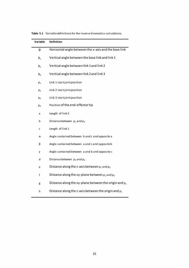
Table 5.1 Variable definitions for the inverse kinematics calculations.

Variable Definition

ψ Horizontal angle between the x-axis and the base link

θ1 Vertical angle between the base link and link 1

θ2 Vertical angle between link 1 and link 2

θ3 Vertical angle between link 2 and link 3

p1 Link 1 start joint position

p2 Link 2 start joint position

p3 Link 3 start joint position

p4 Position of the end-effector tip

a Length of l ink 2

b Distance between p1 and p3

c Length of l ink 1

α Angle contained between b and c and opposite a

β Angle contained between a and c and opposite b

γ Angle contained between a and b and opposite c

d Distance between p3 and p4

e Distance along the z-axis between p1 and p3

f Distance along the xy-plane between p1 and p3

g Distance along the xy-plane between the origin and p1

h Distance along the z-axis between the origin and p1

16

Fig. 5.1 The virtual robot model in a Cartesian coordinate system. Inverse kinematics calculations

find the joint angles (ψ, θ1, θ2 and θ3), given the target position of the end-effector tip (p4).

The points have three components – one for each main axis. For a point p , the components

are denoted xp. , yp. and zp. :

).,.,.( zpypxpp

We want to find joint angles (ψ, θ1, θ2 and θ3), given the target position of the end-effector tip

(p4). The angle ψ can be calculated from the target position projected on the ground:

).,.(2arctan 44 xpyp ( 2arctan = Four-quadrant inverse tangent)

The point 1p , where the first link is connected to the base, can be found since the distance to

the z-axis and the xy-plane is known:

),)sin(,)(cos(1 hggp

17

To find a unique solution for this particular system, the last link is restricted to be vertically

oriented, which reduces the effective DOF from 4 to 3, but has positive side-effect of

maximizing the payload. Since the link lengths are given, the link 3 start joint position,3p , can

easily be found:

).,.,.( 4443 dzpypxpp

The points 1p and 3p are connected via point 2p where link 1 and link 2 are connected. The

point 2p is not known, but the three points create a triangle, where side c is the length of link

1, side a is the length of link 2 and side b is the distance between 1p and 3p :

2

31

2

31

2

3131 )..()..()..(|| zpzpypypxpxpppb

All the sides in the triangle are now known, so the three angles in the triangle ( a , and )

can be calculated with the law of cosines:

bc

acba

2arccos

222

ac

bca

2arccos

222

ab

cba

2arccos

222

Distance along the z-axis between p1 and p3:

zpzpe .. 13

Distance between 1p projected on the xy-plane and 3p projected on the xy-plane:

2

31

2

31 )..()..( ypypxpxpf

To calculate the link angles, the orientation of the triangle must be determined:

),(2arctan1 fe ( 2arctan = Four-quadrant inverse tangent)

18

Finally:

1

1802

90)90(1803

The robot model geometry was based on 3D CAD drawings [24] in the IGES format, retrieved

from the manufacturer (ABB) of the original robot.

5.2 Control

The system we want to control is the actuator in combination with the joint it applies the

torque to. If the actuators were speed driven instead of torque driven, the system would be

very unrealistic, since there are no motors that can produce almost instant speed changes.

Nevertheless, the controllers (and the physics engine) could then be kept fairly simple. A

control signal proportional to the measured error would do a fine job:

mpeKtu )(

where

pK = Proportional gain

Proportional controllers have the required complexity if speed driven actuators are used, but

in reality, a rotating solid body (e.g. a link) cannot be stopped instantaneously, because of its

moment of inertia.

5.2.1 PID Control

The control system in the ABB industrial robots is proprietary software and has been

developed over many years. It would of course be unfeasible to replicate the ABB control

system in this study. The goal is not to find the best type of controller, but to choose a

controller that is good enough to fulfill the purposes with the thesis. The PID controller is the

most common controller [20], and was chosen because it was believed to be good enough to

explore the new robot design paradigm. Fig. 5.2 shows a closed-loop control system with a PID

controller.

19

Fig. 5.2 PID Control System.

PID controllers have three terms with corresponding tuning parameters:

dt

tdeKdtteKteKtu m

d

t

mimp

)()()()(

0

where

pK = Proportional gain

iK = Integral gain

dK = Derivative gain

Increased proportional gain generally results in decreased response time, decreased marginal

stability, improved compensation of process disturbances, but at the same time increased

control signal activity [13].

The integral gain increases the gain at low frequencies. Increased integral gain improves the

compensation of low frequent process disturbances and the steady state accuracy, but

decreases the marginal stability. The integral gain is needed to eliminate steady state errors at

step disturbances [13].

The derivative gain normally results in improved marginal stability and lower damping. It also

means an increased high frequency gain and decreased low frequency gain. The improved

marginal stability means that the gain can be increased to improve performance, but to the

cost of increased frequency gain [13].

Since the computer simulation of the system is of an inherently discrete nature, a discretized

version of the control signal equation was used:

20

0)(,)()(

)()()( 01

1

tet

teteKtteKteKtu m

kmkmd

k

i

imikmpk

where

kt Discretized time ...3,2,1, ktk

t Time Step (See table A.4 in the Appendix)

)()()( kmkkm tytrte

Integral windup is when the integral term in the control signal continues to increase or

decrease, despite that the actuator cannot respond to the change, because it has reached its

maximum or minimum value. With a basic PID controller implementation, this would happen

in this application when the control signal to the joint i actuator goes below i

min or above

i

max . It was counteracted by locking the integral term when the control signal is out of

bounds. The PID controller implementation details can be found in section “PID Controller

Implementation” in Appendix B.

5.2.2 Robot Control System

Fig. 5.3 The robot control system.

21

Fig. 5.3 illustrates an overview of the robot control system. There are four interdependent

control sub-systems – one for each joint. The target position of the end-effector tip is the input

variable to the inverse kinematics system, which calculates the four joint target angles

required to get the end-effector tip to the target position. The four joint control sub-systems

try to minimize the error between the target angles and the actual angles. The forward

kinematics system takes the actual angles as input and calculates the corresponding position of

the end-effector tip.

The performance of the robot is measured with test cases. Each test case has 25 trajectory

points that the end-effector tip is supposed to visit with the aid of a moving target position.

The target position moves from one trajectory point to another according to the current

reference signal characteristic (see section 5.2.3).

The average speed of the end-effector tip when moving between two trajectory points is one

of the task variables, so the time it should take can easily be calculated. At time mt the target

position reaches the other trajectory point and stops. The end-effector momentary positional

error is the distance from the actual position of the end-effector to its target position, and the

positional error is defined as the maximum momentary positional error when

stt m 5.00 . The average positional error is the average of the positional errors for all

trajectory points but the first. The first trajectory point is not counted, because it takes some

time for the initially zero integral term in the PID controller to “settle” at the start of the test

case simulation (see section 5.2.3). The overall average positional error is the average of the

average positional errors for all individuals in an evaluation run (se section 5.3.6).

Fig. 5.4 The joint control sub-system tries to minimize the error between the target angle and the

actual angle.

Fig. 5.4 shows the joint control sub-system. Each control sub-system affects the joint angle via

its torque actuator, controlled by a PID controller. The reference signal is the joint target angle

and the out signal is the actual joint angle.

The forward kinematics (see fig. 5.3), the torque actuators and the joints (see fig. 5.4) are parts

of the physics engine, which is considered as a parameterized black box in this project. The

physics engine takes the torque magnitudes as input and gives the joint actual angles and the

end-effector actual position as output. The physics simulation loop is thus implied and not

shown in the figures.

22

5.2.3 Reference Signal Design

The motivation for modifying the reference signal can be found in the two degree of freedom

design of PID controllers, for example in [4], p. 57, where the reference signal is modified

before it is propagated to the closed loop. In this section, the term reference signal does not

refer to the joint target angle (see fig. 5.4), but to the distance, s , from the initial position of

the end-effector tip to its moving target position (see fig. 5.3). The trajectory of the moving

target position is a straight line from the initial position to the final position, and the reference

signal characteristic tells where on that line the end-effector tip should be as a function of

time.

Fig. 5.5 Step reference signal characteristic (“Step”). The distance, s, is from the initial position of

the end-effector tip to its moving target position. In this case, the final target position is immediately

reached.

Initially, a step reference signal was used (see fig. 5.5). The target position for the end-effector

was changed to its final position in one large step. The system was not guided in how to find its

way to the target position – only the target position was of interest. This resulted in very jerky

trajectories that made the system look unstable.

23

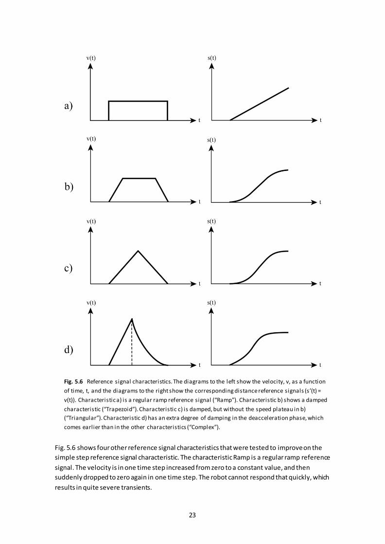
Fig. 5.6 Reference signal characteristics. The diagrams to the left show the velocity, v, as a function

of time, t, and the diagrams to the right show the corresponding distance reference signals (s’(t) =

v(t)). Characteristic a) is a regular ramp reference signal (“Ramp”). Characteristic b) shows a damped

characteristic (“Trapezoid”). Characteristic c) is damped, but without the speed plateau in b)

(“Triangular”). Characteristic d) has an extra degree of damping in the deacceleration phase, which

comes earlier than in the other characteristics (“Complex”).

Fig. 5.6 shows four other reference signal characteristics that were tested to improve on the

simple step reference signal characteristic. The characteristic Ramp is a regular ramp reference

signal. The velocity is in one time step increased from zero to a constant value, and then

suddenly dropped to zero again in one time step. The robot cannot respond that quickly, which

results in quite severe transients.

24

Characteristic Trapezoid has a damped characteristic, where the increase and decrease in

velocity is linear and performed over several time steps. This demands a higher speed during

the plateau phase than in characteristic Ramp, for the same case of trajectory points. This is

realized intuitively, since the distance, s , from the initial position of the end-effector tip (the

first trajectory point) to its final target position (the second trajectory point) equals the areas

under the velocity curves:

dttvdttvs TrapezoidRamp )()(

To get the same area under the velocity curve, the peek speed must be increased when

switching from Ramp to Trapezoid, since the edges of the Ramp velocity characteristic are “cut

off”.

Characteristic Triangular has no speed plateau. The acceleration phase is here stretched out to

half the total time (or distance), and the same goes with the deacceleration. This demands an

even higher peek speed than in characteristic Trapezoid, for the same reason as earlier.

Characteristic Complex is an attempt to create an even smoother deacceleration than in

characteristic Triangular, to further decrease the transient behavior. Once again, this demands

a higher peek speed than in characteristic Triangular.

Fig. 5.7 Acceleration, a, as a function of time, t, for characteristics Triangular (to the left) and

Complex (to the right). The characteristic Complex has an extra degree in the deacceleration phase

to decrease transients.

Fig. 5.7 shows the difference in acceleration between characteristic Triangular and Complex.

The acceleration characteristic to the left shows a constant acceleration half the total duration,

and a constant deacceleration the other half. The characteristic to the right shows a linearly

decreasing deacceleration after 2/5 of the total duration.

25

Fig. 5.8 A complex reference signal characteristic with a smooth deacceleration phase. The

acceleration starts at time ta and the deacceleration at time td. The error measuring starts at time tm.

The distances moved during the acceleration and deacceleration are ∆s a and ∆sd respectively (and

equals the two respective areas in the left diagram). The total distance is ∆s and the maximum

velocity is vmax.

The characteristic Complex is explained in more detail in fig. 5.8. To implement it, we have to

decide when the deacceleration phase should start – the parameter td. The most straight

forward approach is to start the deacceleration after half the total duration:

avg

d

avg

v

stt

v

st

22

where

dt = Start of deacceleration phase

t = Total duration

s = Total distance

avgv = Average speed of the end-effector tip

The deacceleration is smoother than the acceleration and it takes longer time to travel a

certain distance. Expressed in a different way, when the deacceleration starts after half the

total duration, the distance must be closer to the target position than to the start position to

reach the target in time. It was hypothesized that an earlier deacceleration would mean a

lower positional error – up to a certain point, since the resulting acceleration increase during

the first phase would result in jerks, or become unrealistically high for the actuator. It is

beyond the scope of this study to find the optimal start of the deacceleration phase, but the

chosen approach was to let the deacceleration start after half the distance instead of after half

the duration (see the diagram to the right in fig. 5.8):

26

2)(

sts d

da

da

ss

sss

For the sake of simplicity, we assume

0at

With kt representing the discretized time (see section 5.2.1), the velocities during acceleration

and deacceleration become

k

d

kka tt

vtatv max)(

tt

tttt

vtv

m

mk

md

kd

2

2

max )()(

)(

The distances become

s

vtts

avgk

ka

8

)(25)(

2

2

3

54

)(125)(

s

tvssts

kavg

kd

The relation between the start of the deacceleration and the total duration is given by

5

2

m

dd

t

t

t

t

An initial experiment with characteristic Triangular was performed. One optimization run was

made using the procedure outlined in section 5.3, except that the positional errors from all the

25 trajectory points were used in the performance calculations. The average positional error

for 500 new test cases using the winner individual was calculated per trajectory point distance

class. See table A.2 in the Appendix for parameter details.

27

Fig. 5.9 Distance response for different distance limits, ∆s limit. The values on the horizontal axis

correspond to the distances between the trajectory points. With ∆s limit = 0, the average positional

error is severely increased for small movements. With ∆s limit = 45.0 cm or 90.0 cm, the positional

error decreases considerably. Error bars indicate standard error of the mean (n = 500, 496 and 499,

respectively, p < 0.05).

The top curve in fig. 5.9 shows one of the results of the initial optimization experiment. The

term distance limit, ∆slimit, is explained below. The initial 80.0 cm move from the center of the

test case sphere to its perimeter seems to have much worse positional error than for the

neighboring classes 87.6 cm and 75.3 cm. This suggests that the system is not stable, in some

sense, at the start of the test case simulation. It was hypothesized that this was due to the

integral term in the controller, which is zero at the start of the test case simulation. The first

trajectory point was therefore removed in the average positional error calculations in

subsequent experiments.

The same curve also reveals that the average positional error is severely degraded for small

movements. To achieve a more even positional error over a wide range of distances, a speed

reduction scheme was tested. The nominal average speed of the end-effector tip, vavg, which is

one of the task variables, is adjusted if the distance is below a certain threshold, ∆s limit, called

distance limit. Fig. 5.10 shows this functionality.

28

Fig. 5.10 The average speed is reduced for small movements, to a chieve a more even positional

error over a wide range of distances.

Three different settings for the distance limit was tested – 0.0 cm, 45.0 cm and 90.0 cm. Table

A.2 in the Appendix summarizes some of the parameters used in the optimization and

evaluation of the winner. Fig. 5.9 shows the resulting distance responses for the three

different settings.

Fig. 5.11 Detail of distance responses for distance limits 45.0 cm and 90.0 cm. Error bars indicate

standard error of the mean (n = 496 and 499 respectivel y, p < 0.05).

Fig. 5.11 shows a detail of the result for ∆s limit = 45.0 cm and ∆slimit = 90.0 cm. The distance limit

90.0 cm was chosen for subsequent experiments, because it seems to generate a distance

response that is approximately monotonically decreasing and with a small span. It seems

reasonable with a monotonically decreasing distance response, because a constant average

positional error would definitely mean a higher error for small movements, relative to the

distance moved.

29

5.3 Optimization

To find analytical solutions to the optimization problems is not an option, since a physics

engine was used to simulate the kinematics and dynamics of the system, instead of using

explicit equations. To use a genetic algorithm (GA) for the optimization is a better approach,

since they do not require any auxiliary information like gradients and derivatives. We are in

some sense forced to use a black box method, but can we say that a genetic algorithm is a

good method to use in this project? Russell & Norvig [16], p. 119, say that it is not clear under

which conditions GAs perform well. Mitchell [15], p. 155-156, expresses the same opinion, but

states that that many researchers share the intuitions that a GA will have a good chance of

being competitive with or surpassing other black box methods, if:

The search space is large

The search space is not well understood, or known not to be perfectly smooth and

unimodal (consists of a single smooth “hill”)

The fitness function is noisy

The task does not require a global optimum to be found

Since all four conditions were considered satisfied, a genetic algorithm was chosen for the

design optimization.

5.3.1 Genetic Algorithms

Genetic algorithms are methods for optimization and innovation [7], inspired by the process of

biological evolution and implemented in computer software. GAs were invented by John

Holland in the 1960s [11], and have been developed in many different flavors since then. All

living things have evolved, and Hoekstra and Stearns [10] describe the process the following

way: “Adaptive evolution is the process of change in a population driven by variation i n

reproductive success that is correlated with heritable variation in a trait”.

Adaptive evolution occurs in traits that fulfill three conditions:

1. They vary among individuals (genetic diversity).

2. Their variation affects how well those individuals reproduce (natural selection).

3. Some of their variation is determined by genes (heredity).

Individuals that produce many offspring will increase the frequency of its genes in the

population. As this process continues over generations, the population becomes better

adapted. GAs operate on a population of candidate solutions to the optimization problem. A

candidate solution consists of an encoded version of a solution in the form of a bit -string, a list

of values, etc, called chromosome, and a measure of how well the solution solves the problem,

called fitness (fig. 5.13 shows the hierarchical structure of the GA). The fitness will affect the

reproductive success of the individual. This is in contrast to biological evolution, where fitness

30

is a direct measure of the reproductive success. However, the three conditions for adaptive

evolution apply for biological systems as well as for artificial systems like genetic algorithms.

This pseudo code outlines the main steps in a genetic algorithm:

1. Create an initial population.

2. For each individual in the population, evaluate the “goodness” of the corresponding

solution. This is the individual’s fitness.

3. Select parent individuals from the population, using a selection scheme that on

average will favor fitter individuals.

4. Reproduce the parent individuals by applying genetic operators (crossover and

mutation).

5. Replace the old population with the new one.

6. If stop conditions are met, stop, else go to 2.

5.3.2 Encoding

An individual is a candidate solution to the optimization problem, i.e. explicit values for the

design variables. The first step in creating a software implementation of a genetic algorithm is

to decide how to encode the individuals. There are many encoding approaches, e.g. bit -strings,

lists of real-valued numbers, hierarchical structures, etc. The choice of encoding depends

largely on the type of problem to be solved. The way in which candidate solutions are encoded

is a central factor in the success of a genetic algorithm [15], p. 156. As mention earlier, the

design variables differ between the experiments, but let’s say we want to find a good set of

controllers and actuators. There are four controllers and each controller has three parameters,

which are the proportional gain, integral gain and derivative gain. There is one actuator for

each controller, and each actuator has a minimum and a maximum torque. This gives a total of

4 x (3 + 2) = 20 parameters for each individual.

An alphabet with a minimum cardinality (no. of elements in a set, e.g. an alphabet) that still

permits a natural expression of the problem should be selected [6], p. 80. The simplest

encoding is a binary encoding, but since the parameters are naturally expressed as real values

in this project, a real-valued encoding was selected. A real number has an infinite cardinality

( 02 ), but since the computer memory is finite, we have to choose an alphabet with finite

cardinality. There is no natural choice of alphabet, since we don’t know the precision we want,

so for the sake of simplicity, each parameter value was internally represented by 64-bit double

precision values.

Like in nature, a GA individual can be either haploid (single chromosome) or polyploid (more

than one chromosome), but in contrast to nature, haploid individuals are far more common

when it comes to GAs. Both theory and simulation have shown that polyploidy (in combination

with dominance) is useful in non-stationary problems, since it provides a long-term population

memory [6], p. 212. Since this is a stationary problem (does not change during the

31

optimization), a single-chromosome encoding in the form of a list of real-valued numbers, was

consequently chosen.

5.3.3 Selection

To fulfill the condition of natural selection (see condition 2 in section 5.3.1), fitter individuals

must be favored in reproduction.

How do we choose the individuals from the population that will produce offspring and how

many offspring will each parent generate on average? The simplest selection scheme is fitness-

proportionate selection, where the expected no. of times an individual will be selected to

reproduce is that individual’s fitness divided by the average fitness of the population. This

method often suffers from what is known as “premature convergence”, where a small number

of fit individuals take over the population too early [15], p. 167.

To overcome the problem of premature convergence, a selection scheme called stochastic

tournament selection [8] was used. N individuals (tournament size) are chosen at random from

the population. With probability r (selection probability), the fittest individual of the N

individuals is chosen. If the fittest individual was not chosen, the second fittest individual is

chosen with probability r, and so on. If the second last individual was not chosen, the last

individual is chosen. The selection is made with replacement, i.e. we replace the chosen parent

before the second parent is chosen. The two parents produce one offspring by the application

of genetic operators (see section 5.3.4), and the offspring is put into the population of the next

generation.

Elitism is when a number of the fittest individuals in the population are copied and put directly

into the population of the next generation, without applying any genetic operators. This

procedure will guarantee that the best solutions are not destroyed. Many researchers have

found that elitism significantly improves the performance [15], p. 168. In nature, population

sizes tend to follow an approximately logistic curve over time [9], p. 30, but constant

population sizes are most common for GAs. A population size of 20-100 individuals is

commonly used [15], p. 175-176, and a population size of 35 individuals was chosen, two of

which were elite individuals.

5.3.4 Reproduction

An offspring is created by applying genetic operators on the parent individuals. The crossover

operator aims at reusing good building blocks in the next generation, by the combination of

parameters from the two parents. The mutation operator has the role of preserving genetic

diversity and to come up with new useful building blocks, by introducing random changes in

the parameter values.

There are two classes of crossover methods, one where the likelihood of keeping two

parameters on a chromosome together is a positive function of how close the two parameters

are from each other on the chromosome, and one where the parameters are treated

independently of each other. As mentioned in section 5.3.2, there is no natural way to group

32

the parameters in this case, so a crossover method from the second class, called uniform

crossover, was selected.

To create one offspring individual with uniform crossover, one of the parents is chosen by

random to be the basis for the new individual. The genes are then gone through one by one

and with probability pc (crossover probability) the current gene pair (one from each parent

individual) is crossed over. The crossover operation is done by calculating the arithmetic mean

of the two parameter values and then adding a fraction of the difference between the two

parameter values. The stochastic variable σ is calculated from a uniform distribution between

zero and a parameter to the genetic algorithm called gene crossover, gc. Note that for gene

crossover values ≤ 0.5, the resulting gene value, Xc, will be between the two parent gene

values, XA and XB. Specifically, for a gene crossover value of zero, the resulting gene value will

coincide with the arithmetic mean.

),max(),min(5.0

)(2

),0(

BAcBAc

BABA

c

c

XXXXXg

XXXX

X

g

where

= Uniformly distributed stochastic variable

cg = Gene Crossover

cX = Resulting gene value after crossover

AX = Gene Value from parent A

BX = Gene Value from parent B

The motivation for adding the fractional term to the arithmetic mean is to add or keep up the

genetic diversity, but in contrast to the mutation operator, this is done in a more controlled

way. The fractional term goes toward zero when the two parent gene values go toward the

same value, which means that it will not interfere with the convergence of the genetic

algorithm in the same way as the mutation operator might do. The gene crossover value was

found to be non-critical and a value of 0.25 was chosen.

After the crossover procedure, the genes are once again gone through one by one and with

probability pm (mutation probability) the current gene is mutated. The mutation operation is

performed by multiplying the current gene value, X, with a truncated exponentially distributed

expression. The resulting mutated value is denoted Xm. The motivation for the truncated

exponential distribution is to somewhat mimic the mutation of a bit-string integer, which is the

most common encoding. The stochastic variable σ is calculated from a uniform distribution,

using a parameter to the genetic algorithm called gene mutation, gm. The gene mutation value

33

was found to be non-critical and a value of 2.0 was chosen, which will generate a value that is

between ½ and 2 times the original value.

eXX

gg

m

mm

)ln,ln(

where

= Uniformly distributed stochastic variable

mg = Gene Mutation

mX = Mutated gene value.

X = Current gene value

5.3.5 Initialization

To start the optimization process, an initial population must be created. Due to the delicate

balance between the design variables, it is not feasible to initialize the 35 individuals with only

wide range random variables. This straight forward approach was initially tested, but found to

result in robots that performed very poorly. The fact that the links are connected serially to

each other will of course distribute the errors in a multiplicatively way through the links, which

would swing in an “uncontrolled” fashion and counteract each other.

The solution was to create a reasonable set of four base controllers (including the actuator

values) – one for each link – that is used as a starting point in the optimization process. A

prototype individual, holding the values from the base controllers, was repeatedly cloned and

mutated, to produce the individuals for the initial population.

The prospective base controllers were manually tuned in a systematic way. The links were

made speed driven with proportional controllers, instead of torque driven (see the discussion

in section 5.2). This abruptly stops the joints close to zero error, almost without any transient

behavior. The links were then made torque driven and PID controlled one at a time, starting

from the last link, without turning the previous link back to speed driven mode. A Ziegler–

Nichols tuning scheme [21] was used as a starting point and then combined with manual trial

and error tuning. To create a good genetic diversity, the mutation probability for the prototype

individual’s genes was set to 0.8 and the gene mutation (see section 5.3.4) was set to 10.0.

5.3.6 Evaluation of Performance

The performance of the robot is measured with test cases that are randomly generated for

each generation. This suite of test cases is the training set, which is consequently of the same

size as the no. of generations in the run. The average positional error (see section 5.2.2) is the

performance measure for the robot during optimization.

34

Fig. 5.12 An example test case.

Fig. 5.12 gives an idea of how a test case is generated. For the sake of illustration, it is in two

dimensions instead of three. The trajectory points are randomly generated from a sphere with

a center at (x, y, z) = (1.400 m, 0.000 m, 0.900 m) and a radius of 0.800 m. The start position is

at the center of the sphere, the first trajectory point is on the perimeter of the sphere (0.800

m from the start position) and the second trajectory point is on the opposite side of the sphere

from the first trajectory point (0.800 m x 2 = 1.600 m from the first trajectory point). We want

the end-effector to be able to move smoothly between details of large as well as small objects.

The distances between the rest of the points should thus be scale -invariant, which is a

property of a truncated exponential distribution:

1,222

1,

1

1

1

1

1

min1

1 2

minln

kerr

sr

kr

sk

n

k

nn

k

r

s

where

n = No. of trajectory points

35

k = Current trajectory point index, ),1( n

ks = Distance between trajectory point k - 1 and trajectory point k

(or, in case of k = 1, between the start position and the first trajectory point)

mins = Distance between trajectory point n - 1 and trajectory point n

r = Radius of sphere

The parameters were set to n = 25, mins = 0.050 m and r = 0.800 m. Table 5.2 shows the

resulting trajectory point distance classes.

Table 5.2 Trajectory point distance classes.

Distance

Classes

Distances

(m)

∆s1 – ∆s5 0.800 1.600 1.376 1.184 1.018

∆s6 – ∆s10 0.876 0.753 0.648 0.557 0.479

∆s11 – ∆s15 0.412 0.355 0.305 0.262 0.226

∆s16 – ∆s20 0.194 0.167 0.144 0.123 0.106

∆s21 – ∆s25 0.091 0.079 0.068 0.058 0.050

5.3.7 Selection of a Winner

Which individual is the best one in a run? The one with highest fitness for the whole run? A

new test case is randomly generated for each generation, and the test cases differ of course in

how hard they are. The individual with highest fitness for the whole run might be the fittest

one simply because the test case was unusually simple, or because it happened to be very fit

for that particular test case. The generation fitness average will eventually converge after

many generations. The winner individual in a run is chosen to be the one with highest fitness in

a “converged” generation. Exactly which generation to pick is decided after visual inspection of

the fitness vs. generation graph (average and highest) and controller parameter values vs.

generation graph. This policy was chosen to minimize overfitting. That is to say that the

solution generalizes well and will work for a wide range of test cases.

When we have picked the winner using the above procedure, we have to ask: How good is this

individual? The random seed is changed and 500 new test cases are generated and performed.

This suite of 500 test cases is the test set. The average positional error of these test cases are

the measure we use to finally quantify the goodness of the winner individual. But is the winner

really the best one? What if we perform the very same 500 test cases with a similar individual

in a converged generation? Yes, it might actually perform slightly better, but, as Goldberg

36

states in *6+: “The most important goal of optimization is improvement (….) Attainment of the

optimum is much less important for complex systems”.

Instead of this complex procedure, we could of course perform 500 new test cases for each

individual and generation, and then pick the individual with the highest average positional

error in all generations. The more test cases per individual the less the risk of overfitting. With

the computer used in this study (see section 5.4.1), it takes 15 hours and 50 minutes for a 700

generation optimization run with a population size of 35, so it might take a year or at least

months with a more straight forward approach.

5.4 Implementation

5.4.1 Software Tools and Hardware

The computer used for the software development and optimization was a Dell Precision PWS

390 with an Intel® Core™ 2 CPU 6420 @ 2.13 GHz and 3.25 GB RAM. The operating system

used was Microsoft Windows XP Professional Version 2002 SP 3. The software was designed in

the open source UML modeling tool ArgoUML [26] v. 0.30 and implemented using Microsoft

Visual Studio 2008 Professional Edition.

With graphics rendering turned on, the simulation speed is about 60% of real time for a

release build, and with graphics rendering turned off, the simulation speed is about 600% of

real time. See table A.4 in the Appendix for details about parameter values used by the physics

engine for the simulations.

5.4.2 Software Design

The source code is written in Visual C++ and consists of about 3000 lines. Fig. 5.13 shows the

software design of the system.

37

Fig. 5.13 Object oriented UML class hierarchy showing the software design of the system. Fil led

diamonds represent composites and unfil led represent aggregates. The NeuroController class is not

part of the system, but shows the potential for plugging in any kind of c ontroller, using the general

interface of the abstract Controller class. The Evolvable class is an interface for setting and getting

the genome of an object that is to be evolved by an instance of GeneticAlgoritm.

38

6 Experiments

This section describes the experiments performed and their results, to answer the questions

from section 2.2.1. The first subsection shows simulation screen shots.

6.1 Screen Shots

Fig. 6.1-6.3 show screen shots from the simulation, and video clips can be found on [28] or on

YouTube (search on thesis title).

Fig. 6.1 Perspective-view of the simulated robot.

39

Fig. 6.2 Side-view of the simulated robot.

Fig. 6.3 Front-view of the simulated robot.

40

6.2 Q1: How does the reference signal characteristic affect the

positional error?

6.2.1 Experimental setup and analysis

One optimization run was performed for each of the reference signal characteristics Step,

Ramp, Trapezoid (with a = 15 m/s2), Triangular and Complex (see section 5.2.3). Two different

winners were chosen in each optimization run, and evaluation runs were then performed for

these two individuals. One of the two individuals was chosen by comparing the distance

response plots with each of the following criteria: low average positional error, small standard

error, small span and monotonically decreasing.

The distance response plots should be complemented with time domain plots to enable a

thorough analysis (both plots are based on the data from the “winning” evaluation run). To

avoid the effects of possible initial transients in the first generation, the respective test cases

from generation 1 (generation zero being the first) should be used for the time domain plots.

The genetic algorithm framework was implemented for general-purpose optimization and

innovation, and the conventional interpretation of fitness is that a higher fitness is a better

fitness (see section 5.5). We want to minimize the positional error, so we make improvements

by maximizing the negated positional error:

efitness

where

e = Average positional error

Table A.3 in the Appendix summarizes the parameters used for the optimization and

evaluation runs. Fig. 6.4 shows that the lowest and next lowest overall average positional

errors are produced with the reference signal characteristics Step and Complex respectively.

Fig. 6.5-6.8 show the momentary positional error for all five reference signal characteristics for

distance classes 2-25 when the generation 1 test case was used. All reference signal

characteristics but Step produce a fairly smooth trajectory. The transients in the Step

trajectory correspond to the end-effector oscillating around the target position.

Since a smooth trajectory is desired, the reference signal characteristic Complex is chosen as

the winner, and will be used in consecutive experiments, where “the winner in Q1” refers to

the set of evolved controllers and actuators produced with Complex in combination with that

reference signal characteristic. Table 6.1 shows the overall average positional error and total

torque magnitude for the winner. Table A.5-A.9 in the Appendix summarize the optimized

design variable values for all five reference signal characteristics.

41

6.2.2 Results

Fig. 6.4 Distance responses for different reference signal characteristics. Overall average positional

error for the respective reference signal characteristics, from top to bottom in the legend, are 12.6,

7.6, 6.9, 5.8 and 4.1 mm. The trapezoid parameter a is the acceleration/deacceleration in m/s2. Error

bars indicate standard error of the mean (n = 499, 500, 499, 500 and 500, respectively, p < 0.05).

42

Fig. 6.5 Momentary positional error in the time domain for different reference signal characteristics and distance classes 2 -7 (1.600, 1.376, 1.184, 1.018, 0.876

and 0.753 m, respectively). The generation 1 test case was used.

Fig. 6.6 Momentary positional error in the time domain for different reference signal characteristics and distance classes 8 -13 (0.648, 0.557, 0.479, 0.412, 0.355

and 0.305 m, respectively). The generation 1 test case was used.

43

Fig. 6.7 Momentary positional error in the time domain for different reference signal characteristics and distance classes 14 -19 (0.262, 0.226, 0.194, 0.167, 0.144

and 0.123 m, respectively). The generation 1 test case was used.

Fig. 6.8 Momentary positional error in the time domain for different reference signal characteristics and distance classes 20 -25 (0.106, 0.091, 0.079, 0.068, 0.058

and 0.050 m, respectively). The generation 1 test case was used.

44

Table 6.1 Overall average positional error and total torque magnitude for the winning reference

signal characteristic Complex.

Parameter Value

1Q

avge 5.8 mm

1Q

tot 963686 Nm

6.3 Q2: How is the positional error affected when both the

positional error and the total torque magnitude is minimized

at the same time?

6.3.1 Experimental setup and analysis

The total torque magnitude is defined as:

3

0

maxmin ),max(i

ii

tot

where

tot = Total torque magnitude

i

min = Minimum torque magnitude (< 0) for link i

i

max = Maximum torque magnitude (> 0) for link i

It is desirable to minimize the cost and weight of the motors in a robot, which is roughly the

same as minimizing the total torque magnitude, tot . It was hypothesized that tot would

probably increase over the generations in the runs in Q1, since that would give more room for

decreased positional error. Table 6.4 shows that tot increased with a factor of about 11 from

85200 Nm for the set of base controllers to 963686 for the winner in Q1. A compromise

between torque and positional error is necessary, which motivates the following choice of

fitness definition:

11 Q

tot

tot

Q

avge

efitness

45

where

e = Average positional error

1Q

avge = Overall average positional error for the winner in Q1 (see table 6.1)

tot = Total torque magnitude

1Q

tot = Total torque magnitude for the winner in Q1 (see table 6.1)

= Weight to adjust the importance between positional error and torque. A larger value increases the importance of a small total torque magnitude, and vice versa.

A set of six experiments, E1-E6, were performed. A new random training set was generated to

decrease the bias from Q1, while the test set was kept to simplify comparisons. Table 6.2

summarizes the parameters used in the different experiments.

Table 6.2 Parameter values used by the genetic algorithm for the winner in Q1 (Q1) and the Q2

experiments (E1-E6). The parameter in the last row (IK Bug) respresents a software bug in the

inverse kinematics calculations, which was found after E1-E5 were completed.

Parameter Q1 E1 E2 E3 E4 E5 E6

Training Set ID

(Optimization Run)

1 3 3 3 3 3 3

Optimization Generations 400 700 700 1000 1000 1000 1000

Distance Limit, Δs limit (cm) 90.0 90.0 160.0 160.0 160.0 160.0 160.0

Weight, N/A 100 100 5 1 0.2 1

IK Bug Yes Yes Yes Yes Yes Yes No

One optimization run was performed and two different winners were chosen. Evaluation runs

were then performed for these two individuals, and one of the two individuals was chosen,

using the same procedure as in Q1.

E1: The evaluation population size was increased to 700 to capture potential changes later in

the run. The weight, , was set to 100 as a starting point. Fig. 6.9 shows the resulting distance

response. When the distance decreases, the average positional error increases fast for

distances > the distance limit, ∆s limit, and decreases fast for distances < ∆s limit. Table 6.4 shows

that the total torque magnitude, tot , was decreased with a factor of about 44 in relation to

the winner in Q1 and with a factor of about 3.9 in relation to the set of base controllers.

46

E2: The distance limit, ∆slimit, was increased to 160.0 cm to get a smoother distance response.

Fig. 6.9 shows that the average positional error was monotonically decreasing after the

distance limit increase, but was still much higher compared to the winner in Q1. Table 6.4

shows thattot decreased with about 32% in relation to E1.

E3: The weight, , was decreased to 5, to decrease the selection pressure on low total torque

magnitude and enable a higher decrease in average positional error instead. Fig. 6.10 shows

that the distance response for E3 was roughly the same as for E2, and table 6.4 shows that tot

slightly worsened (increased).

E4 and E5: The weight was further decreased from 5 to 1 and 0.2 respectively. Fig. 6.11 shows

that the distance responses were roughly equivalent to the winner in Q1, but table 6.4 shows

that tot decreased with a factor of about 38 and 23 respectively in relation to the winner in

Q1, and with a factor of about 3.3 and 2.0 respectively in relation to the set of base controllers.

Note that tot increased with decreasing weight for E2-E5, as predicted. In conclusion, E4 was

preferred over E5, since the distance responses were roughly equivalent, but in E4 the total

torque magnitude was only 60.0 % of that in E5.

The IK bug: A bug in the inverse kinematics calculations was found after E1-E5 were

completed. The actual link 1 start joint position, with a -122.5 mm y-offset, was used instead of

the point where the rotational axis intersects the common plane (see the 2nd paragraph in

section 5.1). This makes link 1 to look longer than it actually is. The bug was found visually

during simulation, and it looked like the end-effector tip was offset by a small constant amount

parallel to the xy-plane and away from the z-axis. This was confirmed by thorough testing and

debugging, except from the fact that the value is not constant, but depends on the distance

from the origin to the end-effector tip target position.

E6: To get an idea of how the IK bug affected the results, a reevaluation run was perf ormed

with the evolved controllers and actuators from E4, but without the bug. Fig. 6.12 shows that

the overall average positional error was roughly halved, and the standard error was decreased

considerably. A reoptimization run (and subsequent evaluation) was performed with the task

variable values from E4, but without the bug. Fig. 6.13 shows a detail of the distance response,

where the overall average positional error has decreased to 0.083 mm, and fig. 6.12 shows a

comparison to the previous results. The optimized design variable values can be seen in table

A.10 in the Appendix.

47

6.3.2 Results

Table 6.4 Total torque magnitude for the set of base actuators (Base), the winner in Q1 (Q1) and

the Q2 experiments (E1-E6).

Parameter Base Q1 E1 E2 E3 E4 E5 E6

Total Torque

Magnitude (Nm)

85200 963686 22104 14963 18754 25455 42661 28927

Fig. 6.9 Distance responses for experiment E1, E2 and the winner in Q1. E1: When the distance

decreases, the average positional error increases fast for distances > ∆s limit and decreases fast for

distances < ∆s limit. E2: The distance response is monotonically decreasing after the increase of ∆s limit.

Error bars indicate standard error of the mean (n = 499, 499 and 500, respectively, p < 0.05).

48

Fig. 6.10 Distance responses for experiment E2, E3 and the winner in Q1. The distance responses for

E2 and E3 are roughly equivalent. Error bars indicate standard error of the mean (n = 499, 498, and

500, respectively, p < 0.05).

Fig. 6.11 Distance responses for experiment E4, E5 and the winner in Q1. The distance responses

are roughly equivalent. Error bars indicate standard error of the mean (n = 499, 499 and 500,

respectively, p < 0.05).

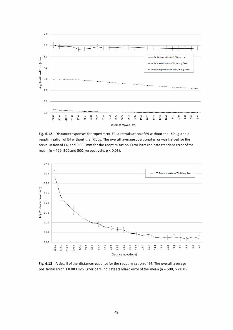
49

Fig. 6.12 Distance responses for experiment E4, a reevaluation of E4 without the IK bug and a

reoptimization of E4 without the IK bug. The overall average positional error was halved for the

reevaluation of E4, and 0.083 mm for the reoptimization. Error bars indicate standard error of the

mean (n = 499, 500 and 500, respectively, p < 0.05).

Fig. 6.13 A detail of the distance response for the reoptimization of E4. The overall average

positional error is 0.083 mm. Error bars indicate standard error of the mean (n = 500, p < 0.05).

50

6.4 Q3: What happens when the load is increased?

6.4.1 Experimental setup and analysis

A 20 kg solid steel load with dimensions (x, y, z) = (168.25, 168.25, 90) mm was attached to the

end-effector. Fig. 6.14 shows a screen shot of the configuration.

Fig. 6.14 Screen shot of the robot carrying a steel load of 20 kg.

An initial evaluation run was performed with the evolved controllers and actuators from E6 in

Q2. The link 3 actuator was not evolved to handle such heavy loads, which swinged back and

forth in an “uncontrolled” fashion. An optimization run (and subsequent evaluation) was

performed with the same setup. The runs were performed with the same parameter values as

in E6 in Q2, except for the 20 kg load. Fig. 6.15 shows how the optimization improved the

overall average positional error with a factor of 100, but the standard error was relatively high

for the longer movements. Despite the extra load, the total torque magnitude decreased with

about 25% to 21603 Nm, and the average positional error dropped from the largest value of

about 11 mm in the 118.4 mm distance class to below 0.05 mm for movements of 19.4 mm

and shorter. The performance for this subset of distance classes is comparable to the

reoptimization in E6 for the same subset. This suggests that a decrease of the weight, ,

51

might give a more stable performance and a lower overall average positional error, but more

expensive (powerful) motors. The optimized design variable values can be seen in table A.11 in

the Appendix.

6.4.2 Results

Fig. 6.15 Distance responses for an experiment where a 20 kg load was attached to the end-

effector. The upper curve shows the result from an evaluation run with the evolved controllers and

actuators from E6 in Q2. The lower curve shows the result after a reoptimization. The overall

average positional error was 269.9 mm and 2.7 mm respectively. Error bars indicate standard error

of the mean (n = 499 and 500 respectively, p < 0.05).

6.5 Q4: How is the positional error affected when the nominal

average speed is changed?

6.5.1 Experimental setup and analysis

The evolved controllers and actuators from E6 in Q2 were used in this experiment, where

evaluation runs were performed with different nominal average speeds. No load was attached

to the end-effector. Fig. 6.16 shows that the overall average positional error increases

dramatically for nominal speeds above the speed the evolved controllers and actuators were

optimized for.

52

6.5.2 Results

Fig. 6.16. Overall average positional errors for different nominal average speeds. The evolved

controllers and actuators from E6 in Q2 were used. The overall average positional error increases

dramatically for nominal speeds above 1.5 m/s, which is the speed the evolved controllers and

actuators were optimized for. Note the log scale on the vertical axis.

53

7 Conclusions

A new robot design paradigm that utilizes evolutionary optimization techniques and advanced

physics simulations was presented and subsequently explored through experimentation. A

piece of software was developed and used to simulate the geometric, kinematic and dynamic

aspects of a serial chain manipulator robot, and to optimize the robot design using a genetic

algorithm. In earlier work, on systems closely related to this project, the complex dynamics

were often simplified. In this project, the dynamics were modeled and simulated with the aid

of a 3D physics engine.

Only predefined robots can be programmed and simulated with current software packages for

offline-programming and robot simulation. It is concluded that such software packages can be

improved by robot design optimization using the software developed in this project, by means

of a genetic algorithm and simulations using a physics engine.

The goals and purposes stated in section 2.1 and 2.2 are considered fulfilled.

This thesis has several novel features. Apart from the use of a physics engine to capture the

complexity of a robotic system, the model geometry was detailed and visually rendered in 3D

during simulation, to aid the model validation and to get a more visually appealing result. It

was possible to detect the bug in the inverse kinematics calculations thanks to this feature.

Distance response analysis was also introduced, which enables a more thorough analysis of the

effects of mechanical resonance. Great effort was put into creating purposef ul and

randomized test cases, which minimize overfitting and facilitates the calculation of useful

performance statistics.

7.1 Restrictions and limitations

The multiphysics engine AgX is proprietary software, which renders a replication of this study

more difficult. On the other hand, the laws of physics are (most likely) static, and an open

source physics engine should produce comparable results. It would have been interesting to

compare some of the performance aspects of the virtual robot to the original, but since ABB

has been cautious with handing out robot data, this has not been possible. The mass, center of

mass and principal moments of inertia for the links have for that reason been calculated from

the 3D CAD model, but have never been verified. The differences in mass properties between

motors with different torque limits could not be captured in the model for the same reason.

The original robot has 6 axes and 6 DOF, which was reduced to 4 axes and 3-4 DOF (dependent

of whether the last link is restricted to be vertically oriented or not) in the robot model. This is

fine for most pick and place tasks, but the full potential of a serial chain manipulator is not

utilized.

The relatively simple PID controller was chosen because it was believed to be good enough to

explore the new robot design paradigm. The results support this view, but the technical

limitations are still evident. If a step disturbance (a sudden push) is introduced during the

54

simulation, it might take the end-effector several seconds to get back on track. A special case

of this is when the end-effector is quite far from the current target trajectory point when the

error measuring period comes to an end and the target position suddenly shift to the next

trajectory point. Sometimes the end-effector lags behind during the whole test case, but

particularly in the beginning of the test case, because the distances between the trajectory

points are longer. This effect can e.g. be seen in the experiment when the controllers and

actuators were optimized with a 20 kg load attached to the end-effector, where the average

positional error dropped considerably for smaller movements. It was hypothesized that an

extra integration term in the controller transfer function might fix this, but there was not

enough time to test the hypothesis.

The main limitation with using a genetic algorithm for the robot design optimization is the

processor time it takes. If a thorough analysis of the results is to be done, this restricts the

complexity of the fitness function and the no. of design variables and constraints.

7.2 Future work

An interesting extension of this work is to optimize the speed or structural parameters like the

link lengths and material properties, to use constraints on the positional errors and the

torques, and to minimize the energy consumption. The parasite-host analogy can be used to

coevolve the test cases with the robot design (with the fitness of the former set to the negated

fitness of the latter), as a strategy to minimize overfitting and the risk of getting stuck in local

optima.

Alternative optimization algorithms that make use of domain-specific knowledge in their

search procedure can be identified and utilized, to increase the optimization speed and to

enable a more complex design optimization.

A robot model with the full 6 DOF and a more complex control system could be created. The

robot can be equipped with a gripper, attached to the last link via a rotational joint, and with a

pair of prismatic joints to articulate the jaw. This would allow for more complex test cases,

designed for specific situations in e.g. industrial or medical environments.

The C++ classes created in this project significantly simplify the development of software

packages for robot simulation and robot design optimization, but much work is still needed to

get a full-fledged robotics software library.

If the traditional robot design paradigm is likened with the selection of the best path in life by

the use of past experience and rules of thumb, the new paradigm does not only give you the

possibility to evaluate the path before you walk it, but to change its direction according to your

destination.

55

8 Acknowledgements

I would like to thank my external supervisor Niklas Melin for his support during the course of

the project, and all other people at Algoryx who have helped me with the intricacies of the

physics engine. I would also like to thank my supervisor at Umeå University, Thomas Hellström,

for his good advice and valuable feedback. Many thanks to Kenneth Bodin and Anders

Backman at Algoryx for introducing me to this challenge. Special thanks to Karolina Kauppi for

your support during my studies leading up to this thesis, and for putting up with me talking

about genetic algorithms and robotics all the time.

56

References

[1] Abdessemed, F., & Benmahammed, K. (2001). A Two-Layer Robot Controller Design Using

Evolutionary Algorithms. Journal of Intelligent and Robotic Systems, 73-94.

[2] Bolmsjö, G. (2006). Industriell Robotteknik (3 ed.). Lund: Studentlitteratur.

[3] Chaiyaratana, N., & Zalzala, A. M. (2002). Time-optimal path planning and control using

neural networks and a genetic algorithm. International Journal of Computational Intelligence

and Applications, 2(2), 153-172.

[4] Crowe, J., Tan, K. K., Lee, T. H., Ferdous, R., Katebi, M. R., Huang, H. P., et al. (2005). PID

Control: New Identification and Design Methods. (M. A. Johnson & M. H. Moradi). London:

Springer.

[5] Gasparetto, A., & Zanotto, V. (2008). A technique for time-jerk optimal planning of robot

trajectories. Robotics and Computer-Integrated Manufacturing, 24(3), 415-426.

[6] Goldberg, D. E. (1989). Genetic Algorithms in Search, Optimization and Machine Learning .

Addison-Wesley.

[7] Goldberg, D. E. (2002). The design of innovation: lessons from and for competent genetic

algorithms. Boston: Kluwer Academic Publishers.

[8] Goldberg, D. E., & Deb, K. (1991). A comparative analysis of selection schemes used in

genetic algorithms. In G. Rawlins, Foundations of Genetic Algorithms. Morgan Kaufmann

Publishers.

[9] Gotelli, N. J. (2001). A Primer of Ecology (3 ed.). Sunderland, Massachusetts: Sinauer

Associates.

[10] Hoekstra, R. F., & Stearns, S. C. (2005). Evolution (2 ed.). Oxford: Oxford University Press.

[11] Holland, J. H. (1992). Adaptation in Natural and Artificial Systems (2 ed.). Cambridge,

Massachusetts: MIT Press.

[12] Lacoursière, Claude (2007). Ghosts and machines: regularized variational methods for

interactive simulations of multibodies with dry frictional contacts. PhD Thesis, Umeå

University.

[13] Lennartson, B. (2002). Reglerteknikens grunder (4 ed.). Lund: Studentlitteratur.

[14] Lundgren, J., Rönnqvist, M., & Värbrand, P. (2010). Optimization. Lund: Studentlitteratur.

[15] Mitchell, M. (1998). An Introduction to Genetic Algorithms. Cambridge, Massachusetts:

MIT Press.

[16] Russell, S. J., & Norvig, P. (2003). Artificial intelligence: a modern approach (2 ed.).

Prentice Hall.

57

[17] Saravanan, R., Ramabalan, S., & Balamurugan, C. (2009). Evolutionary multi-criteria

trajectory modeling of industrial robots in the presence of obstacles. Engineering Applications

of Artificial Intelligence, 22(2), 329-342.

[18] Shiakolas, P. S., Koladiya, D., & Kebrle, J. (2002). Optimum Robot Design Based on Task

Specifications Using Evolutionary Techniques and Kinematic, Dynamic, and Structural

Constraints. Inverse Problems in Science and Engineering, 10(4), 359-375.

[19] Subudhi, B., & Morris, A. S. (2009). Soft computing methods applied to the control of a

flexible robot manipulator. Applied Soft Computing, 9(1), 149-158.

[20] Thomas, B. (1999). Modern reglerteknik (4 ed.). Stockholm: Liber.

[21] Ziegler, J. G., & Nichols, N. B. (1942). Optimum Settings for Automatic Controllers. Trans.

ASME, 64, 759–768.

[22] (n.d.). ABB IRB 4600. Retrieved from

http://www.abb.com/product/seitp327/8c73a1fa083fb25fc12574dc0045a9af.aspx?productLa

nguage=us&country=US&tabKey=2.e=us&country=US&tabKey=2.

[23] (n.d.). ABB IRB 4600 2D CAD Models. Retrieved from

http://search.abb.com/library/ABBLibrary.asp?DocumentID=IRB4600_ALL_IRC5_02_dxfdwg_c

&LanguageCode=en&DocumentPartId=&Action=Launchdirect.

[24] (n.d.). ABB IRB 4600 3D CAD Models. Retrieved from

http://search.abb.com/library/ABBLibrary.asp?DocumentID=IRB4600_40-

255_IRC5_02_IGES_J&LanguageCode=en&DocumentPartId=&Action=Launchdirect.

[25] (n.d.). Algoryx Simulation AB. Retrieved from http://www.algoryx.se.

[26] (n.d.). ArgoUML. Retrieved from http://argouml.tigris.org.

[27] (n.d.). OpenSceneGraph. Retrieved from http://www.openscenegraph.org.

[28] (n.d.). Robot Design Optimization Video Clips. Retrieved from

http://sites.google.com/site/robotdesignoptimization/files.

[29] (n.d.). RobotStudio. Retrieved from

http://www.abb.com/product/seitp327/78fb236cae7e605dc1256f1e002a892c.aspx.

58

Appendix A

Experimental Setup Parameters

Base controllers and actuators

Table A.1 Parameters for the manually tuned base controllers and actuators, which are used as a

starting point in the optimization process.

Link P I D Min Torque (Nm) Max Torque (Nm)

Base Link 45000 150000 7500 -20000 20000

Link 1 270000 700000 30000 -45000 45000

Link 2 30000 100000 5000 -20000 20000

Link 3 300 2000 5 -200 200

Initial experiments

Table A.2 Parameter values used by the genetic algorithm in the initial experiment.

Distance

Limit (cm)

Optimization

Generations

Winner

Generation

Evaluation

Generations

0.0 253 217 500

45.0 239 141 496

90.0 176 153 499

59

Parameters in Q1

Table A.3 Parameter values used by the genetic algorithm in the Q1 experiments.

Parameter Value

Population Size (Optimization Run) 35

Elite Individuals 2

Selection Method Tournament Selection

Tournament Size 2

Selection Probability 0.7

Crossover Type Uniform

Crossover Probability 0.75

Gene Crossover 0.25

Mutation Probability 0.05

Gene Mutation 2.0

Prototype Mutation Probability 0.8

Prototype Gene Mutation 10.0

Include Prototype Individual no

Prototype Individual Base Controller

Optimization Generations 400

Training Set ID (Optimization Run) 1

Evaluation Population Size (1 gen.) 500

Test Set ID, Evaluation Run 1 2

Test Set ID, Evaluation Run 2 2

Nominal average speed, Vavg 1.5 m/s

Distance Limit, Δs limit 90.0 cm

60

Physics Engine Parameters

Table A.4 Parameter values used by the physics engine for the simulations.

Parameter Value

Time Step 1/100 s

Compliance 0 m/N

Damping 1/25 s

Gravity 9.80665 m/s2

Solver Zorro

Result Data

Optimized design variables in Q1

Table A.5 Resulting design variable values in Q1 when optimized with the reference signal

characteristic Complex.

Link P I D Min Torque (Nm) Max Torque (Nm)

Base Link 976409 310398 9536.5 -49684.4 393380

Link 1 7847550 14172800 27433.3 -354273 336598

Link 2 623523 5921.86 5592.14 -214258 72241.6

Link 3 747.555 3194.6 4.01193 -502.821 1775.12

Table A.6 Resulting design variable values in Q1 when optimized with the reference signal

characteristic Triangular.

Link P I D Min Torque (Nm) Max Torque (Nm)

Base Link 1827340 2052410 7500.6 -183678 156675

Link 1 9114430 13289300 37567.6 -59981.7 210822

Link 2 750676 7878.84 5077.87 -256525 40372

Link 3 713.059 11192.9 4.90341 -319.677 747.685

61

Table A.7 Resulting design variable values in Q1 when optimized with the reference signal

characteristic Trapezoid.

Link P I D Min Torque (Nm) Max Torque (Nm)

Base Link 1617610 3927040 6476.33 -37397.6 624713

Link 1 7635340 4403980 20769 -84309.8 310984

Link 2 844292 15189.6 5632.73 -28103 53885.3

Link 3 459.079 3294.74 5.18151 -558.047 2101.84

Table A.8 Resulting design variable values in Q1 when optimized with the reference signal

characteristic Ramp.

Link P I D Min Torque (Nm) Max Torque (Nm)

Base Link 1085840 885362 10567,6 -25509,9 286579

Link 1 10338500 4186660 45288.3 -73068.8 280463

Link 2 640005 1992290 6756.52 -113032 41901.6

Link 3 206.244 3228.24 4.73256 -882.363 766.306

Table A.9 Resulting design variable values in Q1 when optimized with the reference signal

characteristic Step.

Link P I D Min Torque (Nm) Max Torque (Nm)

Base Link 798410 270103 13363.5 -73337.3 61517.8

Link 1 1781720 451084 81334.7 -801632 80445

Link 2 220106 21783.5 7052.23 -20355.8 213449

Link 3 556.432 7399.09 4.25077 -777.469 1769.28

62

Optimized design variables in Q2

Table A.10 Resulting design variable values in the E6 optimization experiment in Q2.

Link P I D Min Torque (Nm) Max Torque (Nm)

Base Link 864048 202279 10876.1 -7246.87 7323.93

Link 1 2810730 7338360 24059 -14943.4 12499

Link 2 1531200 1426490 4394.7 -5713.1 4836.06

Link 3 601.378 13600.6 3.48375 -946.889 573.647

Optimized design variables in Q3

Table A.11 Resulting design variable values in the optimization experiment in Q3.

Link P I D Min Torque (Nm) Max Torque (Nm)

Base Link 1439090 495498 10867.9 -3394.55 3667.43

Link 1 6416170 15415800 29108.5 -13007.5 12209

Link 2 1776550 3406780 2059.98 -4034.08 3713.11

Link 3 11399.8 20940.2 35.5577 -454.149 893.557

63

Appendix B

Robot CAD Drawing

Fig. B.1 CAD Drawing of ABB robot model IRB 4600-40/2.55 [23].

64

Robot Parameters

Table B.1 Physical properties of the virtual robot model,

based on the 3D CAD models in [24] (see also fig. B.1).

When the joint angles are zero and the links are oriented

along the positive x-axis, the link vectors are defined as the

link end joint position minus the link start joint position. A

density of 7850 kg/m3 was used.

Link Mass (kg) Link Vector (mm)

∆x ∆y ∆z

Base 229.6 0 0 159.5

Base Link 112.9 175 -122.5 335.5

Link 1 266.3 1095 -59.1 0

Link 2 545.6 1270 181.6 175

Link 3 13.8 135 0 0

65

Source Code

PID Controller Implementation

Below is the main method in the PIDController class, representing a controller with

proportional, integral and derivative action.

double PIDController::getOutput(double error, double timeStep)

{

if (!saturation)

errorIntegral += error * timeStep;

else

saturation = false;

double errorDerivative = (error - previousError) / timeStep;

double output = proportionalGain * error +

integralGain * errorIntegral +

derivativeGain * errorDerivative;

if (output > maxOutput)

{

output = maxOutput;

saturation = true;

}

else if (output < minOutput)

{

output = minOutput;

saturation = true;

}

previousError = error;

return output;

}