and Physics Chemistry Past and future simulations of NO ... · Chemistry and Physics Past and future simulations of NO2 from a coupled chemistry-climate model in comparison with observations

Atmos. Chem. Phys., 4, 2227–2239, 2004www.atmos-chem-phys.org/acp/4/2227/SRef-ID: 1680-7324/acp/2004-4-2227European Geosciences Union

AtmosphericChemistry

and Physics

Past and future simulations of NO2 from a coupledchemistry-climate model in comparison with observations

H. Struthers1, K. Kreher 1, J. Austin2, R. Schofield3, G. Bodeker1, P. Johnston1, H. Shiona1, and A. Thomas1

1National Institute of Water and Atmospheric Research, Private Bag 50061, Omakau, New Zealand2Geophysical Fluid Dynamics Lab., Princeton Forrestal Campus Rte.1, 201 Forrestal Rd., Princeton, NJ 08542-0308, USA3NOAA Aeronomy Laboratory, 325 Broadway, R/AL8, Boulder CO 80305, USA

Received: 8 June 2004 – Published in Atmos. Chem. Phys. Discuss.: 20 August 2004Revised: 15 November 2004 – Accepted: 15 November 2004 – Published: 22 November 2004

Abstract. Trends in NO2 derived from a 45 year integra-tion of a chemistry-climate model (CCM) run have beencompared with ground-based NO2 measurements at Lauder(45◦ S) and Arrival Heights (78◦ S). Observed trends in NO2at both sites exceed the modelled trends in N2O, the pri-mary source gas for stratospheric NO2. This suggests thatthe processes driving the NO2 trend are not solely dictatedby changes in N2O but are coupled to global atmosphericchange, either chemically or dynamically or both. If CCMsare to accurately estimate future changes in ozone, it is im-portant that they comprehensively include all processes af-fecting NOx (NO+NO2) because NOx concentrations are animportant factor affecting ozone concentrations. Comparisonof measured and modelled NO2 trends is a sensitive test ofthe degree to which these processes are incorporated in theCCM used here. At Lauder the 1980–2000 CCM NO2 trends(4.2% per decade at sunrise, 3.8% per decade at sunset) arelower than the observed trends (6.5% per decade at sunrise,6.0% per decade at sunset) but not significantly different atthe 2σ level. Large variability in both the model and mea-surement data from Arrival Heights makes trend analysis ofthe data difficult. CCM predictions (2001–2019) of NO2 atLauder and Arrival Heights show significant reductions in therate of increase of NO2 compared with the previous 20 years(1980–2000). The model results indicate that the partitioningof oxides of nitrogen changes with time and is influenced byboth chemical forcing and circulation changes.

Correspondence to:H. Struthers([email protected])

1 Introduction

It has been recognised for some time that the reactive speciesNOx are important in the altitude range from approximately20 km to 35 km in determining the concentration of strato-spheric ozone (Crutzen, 1970). NOx destroys ozone throughthe catalytic cycle shown in Reactions (1) and (2).

NO + O3 → NO2 + O2 (1)

NO2 + O → NO + O2 (2)

(net) O3 + O → 2 O2 (3)

In the lower stratosphere (approximately 10 km to 20 km)the most significant influence of NOx is its interaction withthe ClOx and BrOx ozone loss cycles via the formation ofreservoir species ClONO2 and BrONO2. NO2 also reactswith OH (Eq. 4), reducing the HOx concentration and thusinhibiting the HOx catalysed destruction of ozone.

NO2 + OH + M → HNO3 + M. (4)

Oxidation of N2O (Reaction (5)) is the ma-jor source of stratospheric NOy (NO+NO2+NO3+HNO3+2N2O5+HNO4+ClONO2+BrONO2) andhence NOx (Minschwener et al., 1993).

N2O + O(1D) → 2NO. (5)

N2O concentrations are predicted to continue to increaseover the coming century due to anthropogenic surface emis-sions, mostly attributed to agricultural nitrogen fixation(IPCC, 2001; WMO, 1999). Trends in the concentration ofatmospheric N2O for the period 1980 to 1988 have been es-timated to be +0.25±0.05% per year (IPCC (2001), p253).Zander et al.(1994) quote a trend in N2O of +0.33±0.04 %

© 2004 Author(s). This work is licensed under a Creative Commons License.

2228 H. Struthers et al.: Past and future NO2

per year based on remote measurements made at Jungfrau-joch from 1984 to 1996. In contrast to N2O, stratospherichalogen concentrations are expected to decline over the com-ing 50 years as anthropogenic emissions of halogenatedozone-depleting compounds decrease (WMO, 2003). It istherefore important to understand the combined effect ofchanging halogen and NOx concentrations on the future evo-lution of the ozone layer.

Randeniya et al.(2002) studied the effect of increasingN2O and methane on northern mid-latitude ozone columnsfor the period 2000–2100 using the CSIRO two dimensionalchemical model (Randeniya et al., 1997). Their model re-sults show partial recovery of ozone columns through to themiddle of the century due to reductions in halogen concen-trations. This is followed by reduction in ozone columnsfrom 2050 to 2100 whichRandeniya et al.(2002) attributeto increased destruction of ozone by NOx, modulated bythe amount of methane present in the model. Methane con-centrations influence the ozone recovery through the photo-oxidation of methane by halogen radicals in the lower strato-sphere and above 20 km through changes in OH concen-trations leading to changes in the rate of conversion ofNO2 to HNO3. Comparing model ozone profiles for 2100with profiles from 2000,Randeniya et al.(2002) find in-creases in lower stratospheric ozone concentrations over the2000–2100 integration. This is explained by a reduction inthe amount of ozone destroyed by halogen catalytic cycles.However, the recovery in lower stratospheric ozone is offsetby reductions of up to 7% in ozone concentrations in the mid-dle stratosphere due to increased NOx catalytic destruction ofozone.

Modelling future ozone change requires realistic repre-sentations of the anticipated changes in NOx and halogens,in addition to the many other interacting chemical and dy-namical components of the stratospheric system. Three-dimensional coupled chemistry-climate models (CCMs) aredesigned to capture the interaction between climate changeand changes in atmospheric chemistry and are now becom-ing important tools in the prediction of future stratosphericchemistry and dynamics (WMO, 2003). To have confidencein CCM predictions of future stratospheric change, it is nec-essary to assess their reliability. An important methodologyfor validating components of atmospheric chemical modelsis comparison of long time-series of modelled and measuredamounts of trace gases.

Since climate models underpinning all CCMs are chaoticand exhibit unforced variability, comparisons of CCM outputwith observations are necessarily statistical in nature. Al-though comparisons between CCM output and observationson individual days are not meaningful in anything other thana climatological sense, the response of the model to long termforcings should agree with the response observed in the realatmosphere. For this reason, long time-series of observa-tions are required to compare the modelled response to at-mospheric forcings (WMO, 2003).

High quality measurements of NO2 slant column den-sities have been routinely made at Lauder, New Zealand(45◦ S) since 1980 (Johnston and McKenzie, 1989) andArrival Heights, Antarctica (77.8◦ S) since 1982 (McKen-zie and Johnston, 1984; Keys and Johnston, 1986, 1988).The measurements are taken at twilight (sunrise and sun-set). Measuring at a solar zenith angle (SZA) of 90◦ withzenith sky viewing geometry increases the sensitivity of theobserved columns to stratospheric NO2 amounts (Solomonet al., 1987).

Liley et al. (2000) studied the Lauder NO2 data set usingleast squares regression. Indices of QBO, ENSO, solar cycleand the El Chichon and Pinatubo volcanic events in addi-tion to the NO2 annual cycle and secular trend were fitted tothe measured NO2 time-series.Liley et al. (2000) concludedthat the mean 90◦ SZA linear trend in NO2 over Lauder from1980 to 1999 was 5±1% per decade (sunrise trend 5.9±2.4,sunset trend 4.6±1.5 % per decade). These trends are signifi-cantly greater than the trend in N2O estimated to be between2.5% and 3.3% per decade (WMO, 1999). As N2O is thedominant source of stratospheric NO2, this result implies thatthere has been a dynamical or chemical change at southernmid-latitudes which has increased NO2 disproportionately.

Using 1995–2002 Fourier Transform Infra-Red (FTIR)measurements at Kitt Peak (31.9◦ N), Rinsland et al.(2003)derived an NO2 trend of 10.3±5.5% (2σ ) per decade.Lileyet al. (2000) show however, that using short time periods inregression analyses results in large uncertainties in the trendsand therefore the results ofRinsland et al.(2003) cannotbe meaningfully compared with those ofLiley et al. (2000)or those presented here. NO2 data derived from a com-bination of FTIR and differential optical absorption spec-troscopy measurements taken at the Network of the Detec-tion of Stratospheric Change (NDSC) station at Jungfrauo-joch (46.5◦ N) have been analysed and suggest a linearincrease for the period 1985–2001 of 6±2% per decade(WMO, 2003). These results suggest that the NO2 trend be-ing greater than the N2O trend is unlikely to be a local featureat Lauder but is likely to be of global extent.

Fish et al.(2000) used a column model to determine thesensitivity of southern mid-latitude NO2 to changes in strato-spheric temperature, ozone and water vapour. A number ofpossible mechanisms that could change the amount of NO2relative to the amount of N2O were identified:

– direct emission of NOx

– changes in stratospheric circulation

– changes in the shape of the mean NO2 profile

– changes in the partitioning of NOy .

Changes in the partitioning of NOy could arise due tochanges in ozone, temperature, stratospheric water vapourand sulfate aerosol. The focus ofFish et al.(2000) wasto determine whether changes in the partitioning of NOy

Atmos. Chem. Phys., 4, 2227–2239, 2004 www.atmos-chem-phys.org/acp/4/2227/

H. Struthers et al.: Past and future NO2 2229

could explain the observed trend in NO2. The model wasforced with observed changes in ozone, temperature and wa-ter vapour and a 2.5% per decade increase in N2O. The modelfailed to reproduce the observed NO2 trend (model trends+4.0±0.6% per decade at sunrise, +2.0±0.4% per decade atsunset). Including a 20% decrease in stratospheric aerosolin the model forcing gave NO2 trends in agreement with ob-servations (model trends +5.9±0.6% per decade at sunrise,+4.3±0.4% per decade at sunset).

McLinden et al.(2001) used a combination of a three-dimensional chemical transport model, a static columnchemistry model and a radiative transfer model to generateNO2 slant column densities and compared the change in thecolumns over a 20 year time period with the Lauder NO2 ob-servations. Their results show a trend in NO2 of 4.3% perdecade for a prescribed increase in N2O of 3% per decade.Differences in the trends of NO2 and N2O were attributed tothe less than equivalent conversion of N2O to NOy and repar-titioning of NOy due to ozone and halogen changes. The sen-sitivity of their system to temperature and aerosol changeswas also investigated.McLinden et al.(2001) show that thetrend in NO2 vertical column density varies diurnally withlarge changes in the slant column density trends at sunriseand sunset.

Both the studies ofFish et al.(2000) andMcLinden et al.(2001) do not explicitly model the influence of circulationchanges on NO2 amounts. They use rather different modelsand forcings to estimate NO2 slant column density trends.Both conclude that their models reproduce the observed NO2trend but differ in their conclusion as to why there is a dis-tinction between the trends in NO2 and N2O. More work isrequired to fully understand the mechanisms responsible forthe observed difference in trends.

In this paper we calculate NO2 slant column densities forLauder and Arrival Heights using results from the UnifiedModel with Eulerian Transport and Chemistry (UMETRAC),a three-dimensional CCM. NO2 values are derived from a 40year simulation of the model, (1980 to 2019). Model NO2slant columns for Lauder and Arrival Heights are comparedwith the measurements for the period 1980 to 2000 to testthe model’s ability to reproduce the greater than than pro-portional increase in NO2 relative to N2O that has been ob-served in the measurements. The UMETRAC predictions ofNO2 trends at Lauder and Arrival Heights for the period 2001to 2019 are introduced and discussed in light of the 1980 to2000 model/observation comparison.

2 Measurements

The NO2 measurement technique and retrieval algorithmare discussed byJohnston and McKenzie(1989) andLileyet al. (2000). The automated scanning spectrometers mea-sure wavelengths from 435 nm to 450 nm with a spectral res-olution of 1.2 nm. Twilight spectra are ratioed with mid-

day reference spectra to remove Fraunhofer absorption linespresent in sunlight. Each twilight measurement is also cor-rected for the Ring effect (Grainger and Ring, 1963) usingthe “offset Ring” approach (Johnston and McKenzie, 1989).

The instruments at Lauder and Arrival Heights have beencalibrated and intercompared to the standard required of theNetwork for Detection of Stratospheric Change (NDSC).

Model ozone and 20 hPa temperatures are also comparedwith measurements as changes in these quantities have beenidentified byFish et al.(2000) andMcLinden et al.(2001) asbeing important in determining changes in NO2. The 20 hPalevel approximately coincides with the peak in the NO2 mix-ing ratio and was therefore used as the level for the temper-ature comparison. It has been shown (Keys and Johnston,1986) that NO2 slant columns measured over Arrival Heightscorrelate strongly with stratospheric temperatures.

Modelled ozone data are compared with the NIWA assim-ilated ozone data-set (Bodeker et al., 2001). This data-setcontains total column ozone values derived from a combina-tion of TOMS and GOME satellite measurements which arecorrected against the global ground-based network of Dob-son spectrophotometers. NCEP/NCAR (Kalnay et al., 1996)20 hPa temperature data are used for the temperature com-parison.

3 Least squares regression analysis

Linear trends in the NO2 slant column density time-seriesare calculated using a least squares regression model. Theregression model has been applied to ozone time-series inprevious studies (Bodeker et al., 1998, 2001).

A number of forcings are known to influence the southernmid-latitude stratosphere:

– El Nino southern oscillation (ENSO)

– Quasi-biennial oscillation (QBO)

– 11 year solar cycle

– Volcanic injection of sulfate aerosol and water vapour.For the time period 1980–2000, two volcanic eventsoccurred which were significant for the southern mid-latitude stratosphere, El Chichon (1982) and Pinatubo(1991).

The regression model is designed to allow fitting of indicesfor the above forcings, in addition to fitting the seasonal cycleand linear trend in the data. Inclusion of additional, higherorder Fourier components to the basis function describingthe trend allows the model to fit seasonally varying trendsin the data. A description of the indices for the externallyforced basis functions (ENSO, QBO, solar cycle and volca-noes) within the regression model is given inBodeker et al.(1998).

www.atmos-chem-phys.org/acp/4/2227/ Atmos. Chem. Phys., 4, 2227–2239, 2004


The residual terms from the fitting may be autocorrelatedleading to an underestimation of the uncertainty in the re-sulting trends. An autocorrelation model is applied to theresiduals to correct for any autocorrelation.

For the observational record, all basis functions (ENSO,QBO, solar cycle volcanoes) are included in the regres-sion analysis. For the model time-series, only the ENSOand QBO terms are applied (in addition to the annual cy-cle (offset) and linear trend). The model does not include an11 year solar cycle and uses an invariant, background sul-fate aerosol field. The non-orographic gravity wave forcingscheme within the model produces a QBO in the tropicalzonal winds (Scaife et al., 2000). Mean, equatorial zonalwinds produced by the model at 50 hPa were used to gener-ate the model QBO basis function.

4 Model description

4.1 The coupled chemistry-climate model

UMETRAC uses the Met Office’s Unified Model (UM)(Cullen and Davies, 1991) as the underlying climate model.The model has a resolution of 3.75◦ (longitude), 2.5◦ (lat-itude) and 64 vertical levels from the surface to 0.01 hPa.A non-orographic gravity wave forcing scheme (Warner andMcIntyre, 1999) is used to parameterise gravity wave break-ing.

The UMETRAC chemistry scheme is based on a familiesapproach (Austin, 1991). 15 chemical tracers and one dy-namical tracer are advected by the model. The dynamicaltracer is used to parameterise the long lived species H2O,CH4, Cly, Bry, H2SO4 and NOy. The chemistry schemeincludes 65 gas phase chemical reactions, 9 heterogeneouschemical reactions and 27 photolysis reactions. A PSCscheme based on liquid ternary solutions and water ice anda simple sedimentation scheme are also part of the model.Chemical reaction rates are taken fromDeMore et al.(1997)andSander et al.(2000).

There are some differences between the UMETRAC con-figuration used in this paper and the configuration used inprevious work (Austin and Butchart, 2003). These includea new tracer advection scheme, the chemistry scheme beingapplied over the whole vertical domain of the model ratherthan being restricted to the stratosphere and lower meso-sphere, two additional chemical tracers are included (CO andCH3OOH) and an extension of the chemical reaction set.

Water vapour concentrations in the chemistry module weretaken from the UARS reference atmosphere project (URAP)reference atmosphere (http://code916.gsfc.nasa.gov/Public/Analysis/UARS/urap/home.html) and held fixed over the in-tegration. Stratospheric aerosol was derived from the aerosolsurface area densities given in Table 8.8 ofWMO (1991).Again, the aerosol amounts were held constant over themodel integration.

Importantly for this study, the rate of increase of N2O wasfixed at +2.6% per decade for the entire length of the inte-gration (1980 to 2019). The model uses a parameterisationto determine the amount of NOy present at each time step,based on the transport of a conserved tracer and the com-pact relationships ofPlumb and Ko.(1992). In a subsequentstep, the model partitions the NOy according to the chemi-cal scheme within the model. The global rate of increase ofNOy is fixed to the rate of increase in N2O (2.6% per decade)but local rates of increase in NOy may differ from this in re-sponse to circulation changes in the model via changes in theconserved tracer.

Results used in this paper come from a 45 year integrationof UMETRAC (1975 to 2019), with the first five years usedas model spinup. The IS92a IPCC scenario was used to deter-mine greenhouse gas concentrations (CO2, CH4 and N2O).Halogen concentrations were taken from theWMO (1999)assessment. Observed sea surface temperatures (SST) wereused in the model from 1975 to 1999. For years after 1999,sea surface temperature data were taken from simulations ofa coupled ocean-atmosphere version of the UM.

Global fields of the 15 chemical tracers, 6 long-livedspecies and chemical families and temperature are outputfrom UMETRAC every five days at 00:00 UT. These dataare used as input for the UMETRAC column model whichproduced NO2 profiles.

4.2 UMETRAC column model

Since the output from the 45 year UMETRAC integrationprovided only concentrations of chemical families, an off-line chemical model was required to determine the parti-tioning amongst the chemical families output from the fullthree-dimensional model. Vertical profiles of chemical fam-ilies and daily mean temperature for the grid boxes coveringLauder and Arrival Heights were extracted from the UME-TRAC output and used as initial conditions for the columnmodel. The chemistry scheme within the column modelis identical to the chemical scheme used in the full three-dimensional model.

The column model was run for one day to establish theNO2 diurnal cycle. The chemical time step was reduced from15 min in the full three-dimensional model to 3 min for thecolumn model. This allows NO2 profiles to be calculatedwith a SZA resolution of 1◦, ensuring the diurnal cycle ofthe model is adequately represented in the radiative transfermodel for the calculation of slant column densities.

Over the one day integration of the column model, theNO2 concentrations will differ from the corresponding NO2concentrations calculated in the full UMETRAC model dueto the use of the diurnal mean temperature profile. Usingsimple sensitivity tests, it can be shown that these inconsis-tencies between the full model and the off-line column modelhave little impact on the slant column densities due to the


http://code916.gsfc.nasa.gov/Public/Analysis/UARS/urap/home.html

http://code916.gsfc.nasa.gov/Public/Analysis/UARS/urap/home.html


0

4

8

12

16

0

4

8

12

16

1980 1982 1984 1986 1988 1990 1992 1994 1996 1998 20000

4

8

12

16

NO

2 sl

ant

colu

mn

(1016

mol

ec c

m-2

)

90o pm

90o am 90o am

90o pm

Aug/Sept 19880

4

8

12

16

NO

2 sl

ant

colu

mn

(1016

mol

ec c

m-2

)

Aug/Sept 1988ObservationsUMETRAC

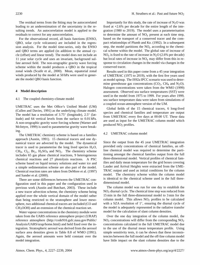
Fig. 1. Comparison of UMETRAC modelled (black) and observed (grey) 90◦ NO2 slant column density time-series for Lauder (1980–2000). Upper left panel sunrise, lower left panel sunset. A subset of the data is shown in the right hand panels to illustrate the estimatederrors in the model and observed values and the data frequency.

small diurnal temperature variations in the lower and middlestratosphere where the slant column weighting is greatest.

Finally, the NO2 profiles calculated by the column modelwere interpolated from terrain following model levels to alti-tude surfaces from the ground to 72 km in 500 m steps.

4.3 Radiative transfer model

In transforming the measured NO2 slant column densities tovertical column densities, some prior knowledge of the verti-cal profile shape is required (McKenzie et al., 1991). Assum-ing a vertical profile shape in an air mass factor calculationcan lead to errors due to the seasonal and annual variation ofthe true vertical profile, which the assumed profile shape maynot capture. In this work the slant column densities were cal-culated using the radiative transfer model (RTM) developedby Schofield et al.(2003) from the profiles determined byUMETRAC. This allows direct comparison of slant columndensities derived from UMETRAC output with observations.

The RTM constructs a model atmosphere using tempera-ture, pressure and ozone profiles taken from the UMETRACcolumn model. The RTM uses a spherically curved atmo-spheric geometry, divided into discrete atmospheric shells.For this study, ninety 1 km thick shells were used to de-scribe the model atmosphere. The effects of refraction,Rayleigh scattering, Mie scattering and molecular absorp-tion at a wavelength of 450 nm (see Sect.2) were includedin the RTM path description of the NO2 zenith-sky measure-ment. Refractive indices were taken fromBucholtz(1995).A single scattering approximation was used for the zenith-sky viewing geometry.

The diurnal variation of the NO2 profile adds complexityto the slant column density calculation. The variation of theNO2 abundance along the slant path with solar zenith an-gle is explicitly taken into account. NO2 profiles at 1◦ so-lar zenith angle intervals between 30◦ and 97◦ calculated by

the UMETRAC column model were used to construct a two-dimensional profile grid. This was then interpolated to therelevant altitude and solar zenith angle along each scatteredlight path. The slant column for the solar zenith angle of90◦ was calculated by integrating the amount of NO2 overall light paths scattered from the zenith.

5 Discussion of Lauder results

5.1 Lauder NO2 time-series

The time-series of modelled and measured NO2 slant col-umn densities for Lauder are shown in Fig.1. The model re-sults capture the absolute value of the NO2 slant columns andthe amplitudes of the seasonal cycle in NO2 for both sunriseand sunset very well. The model in general underestimatesthe observed slant columns for both the sunrise and sunsettime-series. The agreement for the sunset case is somewhatworse than the sunrise which implies that the model has asuppressed NO2 diurnal cycle.

The right hand panels of Fig.1 show a subset of the datato illustrate more clearly the data frequency and estimated er-rors. The time period (August and September 1988) was cho-sen as representative of the whole data record, excluding thetime periods affected by the El Chichon and Pinatubo erup-tions. Observation errors are estimated at 0.2×1016 moleccm−2 + 5% of the observed value. This prescription comesfrom an analysis of the error characteristics of the measuredspectra and the retrieval algorithm used to derive the NO2slant column measurements.

The regression model used to fit the time-series requiresan error estimate associated with each input data point. Inthe absence of an ab initio estimate of the error in the modelNO2 slant column densities, errors are prescribed using thesame error estimate as that used for the observations.



0

4

8

12

16

-9

-6

-3

0

3

6

9

1980 1982 1984 1986 1988 1990 1992 1994 1996 1998 2000-9

-6

-3

0

3

6

NO

2 co

lum

n re

sidu

al (

1016

mol

ec c

m-2

)

Timeseries (mean annual cycle removed)

90o pm

90o am

90o am

90o pm

60 120 180 240 300 360Day number

0

4

8

12

16

Mea

n N

O2

slan

t co

lum

n (1

016 m

olec

cm

-2)

Mean annual cycle

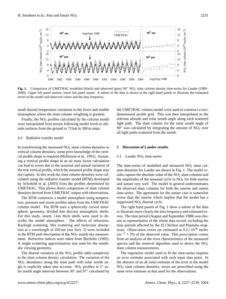
Fig. 2. Lauder NO2 slant column density time-series with the mean annual cycle removed. Observed residuals (grey) have been offset by+3 units and the model residuals (black) offset by−3 units for clarity. The time-series have been thinned by retaining data only when bothobservation and model values are present on a given day. Right hand panels show the mean annual cycles (1980–2000) for sunrise (top) andsunset (bottom).

-5

-2.5

0

2.5

5

7.5

10

Lin

ear

tren

d (p

erce

nt p

er d

ecad

e)

-5

-2.5

0

2.5

5

7.5

10

Observations (1981-2000)Model (1980-2000)Model (2000-2019)

NO

2 (am

)

NO

2 (pm

)

N2O

(gl

obal

)

Ozo

ne

Tem

pera

ture

(K

per

dec

ade)

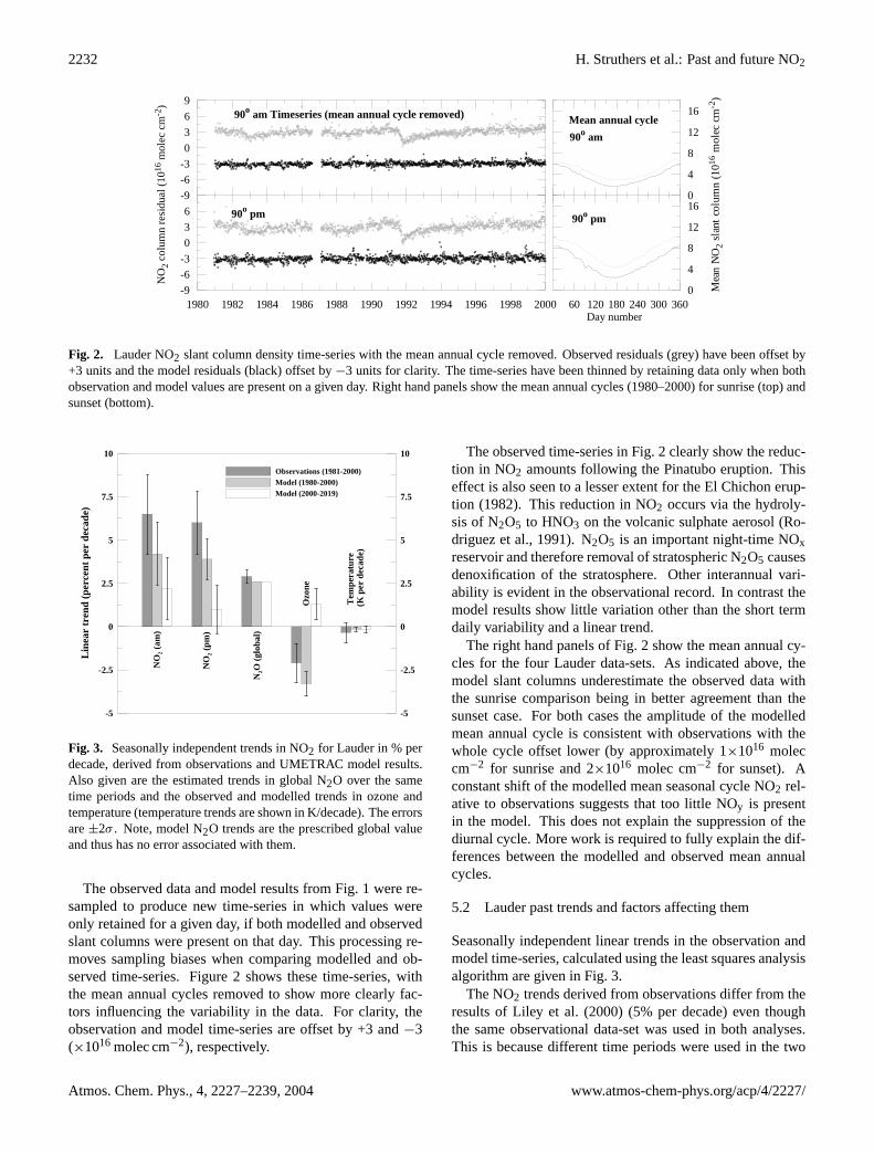
Fig. 3. Seasonally independent trends in NO2 for Lauder in % perdecade, derived from observations and UMETRAC model results.Also given are the estimated trends in global N2O over the sametime periods and the observed and modelled trends in ozone andtemperature (temperature trends are shown in K/decade). The errorsare±2σ . Note, model N2O trends are the prescribed global valueand thus has no error associated with them.

The observed data and model results from Fig.1 were re-sampled to produce new time-series in which values wereonly retained for a given day, if both modelled and observedslant columns were present on that day. This processing re-moves sampling biases when comparing modelled and ob-served time-series. Figure2 shows these time-series, withthe mean annual cycles removed to show more clearly fac-tors influencing the variability in the data. For clarity, theobservation and model time-series are offset by +3 and−3(×1016 molec cm−2), respectively.

The observed time-series in Fig.2 clearly show the reduc-tion in NO2 amounts following the Pinatubo eruption. Thiseffect is also seen to a lesser extent for the El Chichon erup-tion (1982). This reduction in NO2 occurs via the hydroly-sis of N2O5 to HNO3 on the volcanic sulphate aerosol (Ro-driguez et al., 1991). N2O5 is an important night-time NOxreservoir and therefore removal of stratospheric N2O5 causesdenoxification of the stratosphere. Other interannual vari-ability is evident in the observational record. In contrast themodel results show little variation other than the short termdaily variability and a linear trend.

The right hand panels of Fig.2 show the mean annual cy-cles for the four Lauder data-sets. As indicated above, themodel slant columns underestimate the observed data withthe sunrise comparison being in better agreement than thesunset case. For both cases the amplitude of the modelledmean annual cycle is consistent with observations with thewhole cycle offset lower (by approximately 1×1016 moleccm−2 for sunrise and 2×1016 molec cm−2 for sunset). Aconstant shift of the modelled mean seasonal cycle NO2 rel-ative to observations suggests that too little NOy is presentin the model. This does not explain the suppression of thediurnal cycle. More work is required to fully explain the dif-ferences between the modelled and observed mean annualcycles.

5.2 Lauder past trends and factors affecting them

Seasonally independent linear trends in the observation andmodel time-series, calculated using the least squares analysisalgorithm are given in Fig.3.

The NO2 trends derived from observations differ from theresults ofLiley et al. (2000) (5% per decade) even thoughthe same observational data-set was used in both analyses.This is because different time periods were used in the two



0 60 120 180 240 300 360Day number

-10

-5

0

5

10

15

20

NO

2 tr

end

(% p

er d

ecad

e)

0 60 120 180 240 300 360Day number

-10

-5

0

5

10

15

20

NO

2 tr

end

(% p

er d

ecad

e)90oam 90opm

ObservationsUMETRAC

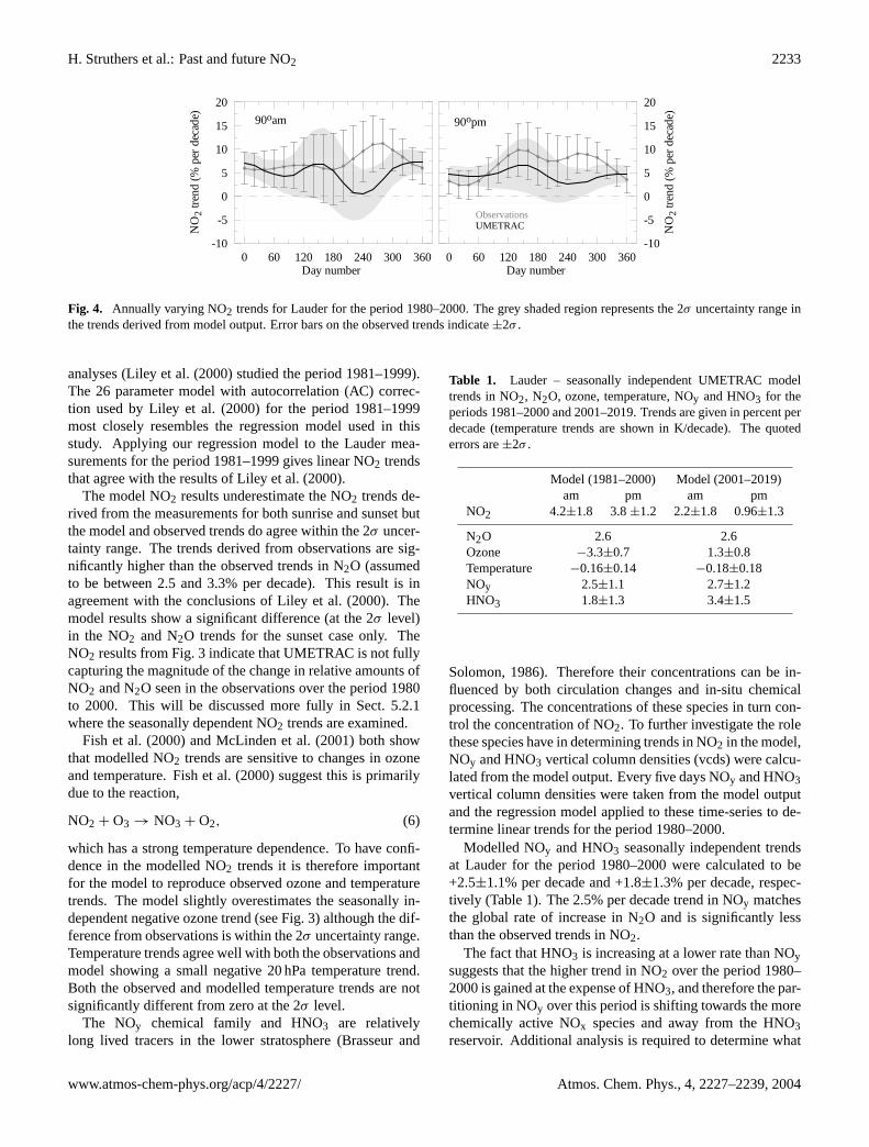
Fig. 4. Annually varying NO2 trends for Lauder for the period 1980–2000. The grey shaded region represents the 2σ uncertainty range inthe trends derived from model output. Error bars on the observed trends indicate±2σ .

analyses (Liley et al. (2000) studied the period 1981–1999).The 26 parameter model with autocorrelation (AC) correc-tion used byLiley et al. (2000) for the period 1981–1999most closely resembles the regression model used in thisstudy. Applying our regression model to the Lauder mea-surements for the period 1981–1999 gives linear NO2 trendsthat agree with the results ofLiley et al. (2000).

The model NO2 results underestimate the NO2 trends de-rived from the measurements for both sunrise and sunset butthe model and observed trends do agree within the 2σ uncer-tainty range. The trends derived from observations are sig-nificantly higher than the observed trends in N2O (assumedto be between 2.5 and 3.3% per decade). This result is inagreement with the conclusions ofLiley et al. (2000). Themodel results show a significant difference (at the 2σ level)in the NO2 and N2O trends for the sunset case only. TheNO2 results from Fig.3 indicate that UMETRAC is not fullycapturing the magnitude of the change in relative amounts ofNO2 and N2O seen in the observations over the period 1980to 2000. This will be discussed more fully in Sect.5.2.1where the seasonally dependent NO2 trends are examined.

Fish et al.(2000) andMcLinden et al.(2001) both showthat modelled NO2 trends are sensitive to changes in ozoneand temperature.Fish et al.(2000) suggest this is primarilydue to the reaction,

NO2 + O3 → NO3 + O2, (6)

which has a strong temperature dependence. To have confi-dence in the modelled NO2 trends it is therefore importantfor the model to reproduce observed ozone and temperaturetrends. The model slightly overestimates the seasonally in-dependent negative ozone trend (see Fig.3) although the dif-ference from observations is within the 2σ uncertainty range.Temperature trends agree well with both the observations andmodel showing a small negative 20 hPa temperature trend.Both the observed and modelled temperature trends are notsignificantly different from zero at the 2σ level.

The NOy chemical family and HNO3 are relativelylong lived tracers in the lower stratosphere (Brasseur and

Table 1. Lauder – seasonally independent UMETRAC modeltrends in NO2, N2O, ozone, temperature, NOy and HNO3 for theperiods 1981–2000 and 2001–2019. Trends are given in percent perdecade (temperature trends are shown in K/decade). The quotederrors are±2σ .

Model (1981–2000) Model (2001–2019)am pm am pm

NO2 4.2±1.8 3.8±1.2 2.2±1.8 0.96±1.3

N2O 2.6 2.6Ozone −3.3±0.7 1.3±0.8Temperature −0.16±0.14 −0.18±0.18NOy 2.5±1.1 2.7±1.2HNO3 1.8±1.3 3.4±1.5

Solomon, 1986). Therefore their concentrations can be in-fluenced by both circulation changes and in-situ chemicalprocessing. The concentrations of these species in turn con-trol the concentration of NO2. To further investigate the rolethese species have in determining trends in NO2 in the model,NOy and HNO3 vertical column densities (vcds) were calcu-lated from the model output. Every five days NOy and HNO3vertical column densities were taken from the model outputand the regression model applied to these time-series to de-termine linear trends for the period 1980–2000.

Modelled NOy and HNO3 seasonally independent trendsat Lauder for the period 1980–2000 were calculated to be+2.5±1.1% per decade and +1.8±1.3% per decade, respec-tively (Table1). The 2.5% per decade trend in NOy matchesthe global rate of increase in N2O and is significantly lessthan the observed trends in NO2.

The fact that HNO3 is increasing at a lower rate than NOysuggests that the higher trend in NO2 over the period 1980–2000 is gained at the expense of HNO3, and therefore the par-titioning in NOy over this period is shifting towards the morechemically active NOx species and away from the HNO3reservoir. Additional analysis is required to determine what



fraction of the difference between the NOy and HNO3 trendscan be attributed to circulation changes and what fraction ofthe difference is due to chemical forcing.

5.2.1 Annually varying NO2 trends

Figure4 shows the seasonally dependent NO2 trends calcu-lated by adding two Fourier components (annual and semi-annual) to the basis function describing the trend in the re-gression model (Bodeker et al., 1998). The trends are takenas a percentage of the daily mean. That is, the trends are cal-culated in units of molec cm−2 per decade and then taken asa percentage of the annual mean over the whole period (givenin the right hand panels of Fig.2).

The results shown in Fig.4 indicate that for much of theyear, the model NO2 trends are in good agreement with thetrends derived from observations. The greatest differencesoccur in spring time for both sunrise and sunset cases, wherethe model is underestimating the trends seen in the observa-tions. The model underestimation of the springtime increasein NO2 is the cause of the model failing to fully reproducethe difference between the seasonally independent NO2 andN2O trends for the period 1980 to 2000 (see Fig.3).

The same regression model (with seasonally dependentbasis functions for the linear trend term) was used to fit themodelled and measured ozone and 20 hPa temperature time-series. The seasonal cycle in ozone and 20 hPa tempera-ture trends was reproduced well by the model (not shown).Therefore ozone and temperature were ruled out as the causeof the model underprediction of springtime NO2 trends.

Differences in the timing of the vortex breakup and subse-quent mixing of vortex and mid-latitude air can also be ruledout as the cause of the differences in the modelled and ob-served Lauder springtime NO2 trends. Generally, the mixingof vortex air to mid-latitudes occurs in early summer (Ajtic ,2004), from approximately day 288 (15 October) which isafter the maximum in the trend differences (approximatelyday 240–28 August). The model, if anything, tends to delaythe breakup of the Antarctic polar vortex further reinforcingthis conclusion.

Stratospheric NO2 amounts have been shown to be sen-sitive to changes stratospheric water vapour (Fish et al.,2000; McLinden et al., 2001). Measured trends in strato-spheric water vapour are uncertain (SPARC, 2000; Rosenlofet al., 2001; Randel et al., 2004). In this study, UMETRACused a fixed climatology of stratospheric water vapour whichmay contribute to the discrepancy between modelled and ob-served NO2 trends.

5.3 Model predictions: Lauder 2001–2019

Table 1 (and Fig.3) compares the seasonally independent,predicted NO2 model trends for the period 1 January 2001to 31 December 2019 with the model trends for the period 1January 1980 to 31 December 2000.

Predicted NO2 trends (2001–2019) are lower than thetrends for the period 1980–2000 even though the N2O trendstays the same. This difference is statistically significant atthe 2σ level for the sunset case. Both the absolute and rela-tive differences between trends for the two periods are largerfor the sunset case.

NOy and HNO3 vertical column density trends for the pe-riod 2001–2019 are compared with the 1980–2000 trends inTable1. It is clear from Table1 that the shift in NO2 trendsfrom 1980–2000 to 2001–2019 is associated with a changein HNO3 trends between the two periods. As was the casefor the 1980–2000 period, it is a change in partitioning ofthe NOy that is resulting in the less than proportional rate ofincrease in NO2 relative to NOy (and N2O) rather than localchanges in the amount of NOy relative to N2O.

Quantification of how chemical changes (for examplehalogen loading and ozone) and circulation changes affectNOy partitioning requires additional analysis of model re-sults which is outside the scope of this paper.

It should be reiterated that the results shown here are fora solar zenith angle of 90◦. McLinden et al.(2001) showthat the trends in NO2 vary significantly with solar zenithangle. It is therefore to be expected that different conclusionsmay be drawn from analysis of data at different solar zenithangles.

6 Discussion of Arrival Heights results

6.1 Arrival Heights NO2 time-series

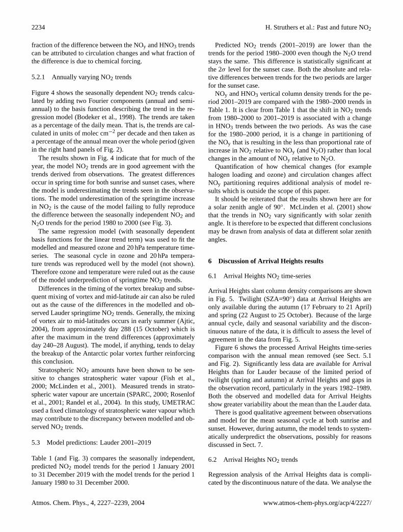
Arrival Heights slant column density comparisons are shownin Fig. 5. Twilight (SZA=90◦) data at Arrival Heights areonly available during the autumn (17 February to 21 April)and spring (22 August to 25 October). Because of the largeannual cycle, daily and seasonal variability and the discon-tinuous nature of the data, it is difficult to assess the level ofagreement in the data from Fig.5.

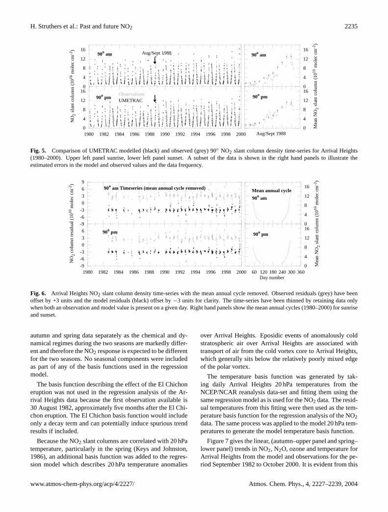
Figure6 shows the processed Arrival Heights time-seriescomparison with the annual mean removed (see Sect.5.1and Fig.2). Significantly less data are available for ArrivalHeights than for Lauder because of the limited period oftwilight (spring and autumn) at Arrival Heights and gaps inthe observation record, particularly in the years 1982–1989.Both the observed and modelled data for Arrival Heightsshow greater variability about the mean than the Lauder data.

There is good qualitative agreement between observationsand model for the mean seasonal cycle at both sunrise andsunset. However, during autumn, the model tends to system-atically underpredict the observations, possibly for reasonsdiscussed in Sect.7.

6.2 Arrival Heights NO2 trends

Regression analysis of the Arrival Heights data is compli-cated by the discontinuous nature of the data. We analyse the



0

4

8

12

16

0

4

8

12

16

1980 1982 1984 1986 1988 1990 1992 1994 1996 1998 20000

4

8

12

16

NO

2 sl

ant

colu

mn

(1016

mol

ec c

m-2

)

90o pm

90o am 90o am

90o pm

Aug/Sept 19880

4

8

12

16

Mea

n N

O2

slan

t co

lum

n (1

016 m

olec

cm

-2)

Aug/Sept 1988

ObservationsUMETRAC

Fig. 5. Comparison of UMETRAC modelled (black) and observed (grey) 90◦ NO2 slant column density time-series for Arrival Heights(1980–2000). Upper left panel sunrise, lower left panel sunset. A subset of the data is shown in the right hand panels to illustrate theestimated errors in the model and observed values and the data frequency.

0

4

8

12

16

-9

-6

-3

0

3

6

9

1980 1982 1984 1986 1988 1990 1992 1994 1996 1998 2000-9

-6

-3

0

3

6

NO

2 co

lum

n re

sidu

al (

1016

mol

ec c

m-2

)

Timeseries (mean annual cycle removed)

90o pm

90o am

90o am

90o pm

60 120 180 240 300 360Day number

0

4

8

12

16

Mea

n N

O2

slan

t co

lum

n (1

016 m

olec

cm

-2)

Mean annual cycle

Fig. 6. Arrival Heights NO2 slant column density time-series with the mean annual cycle removed. Observed residuals (grey) have beenoffset by +3 units and the model residuals (black) offset by−3 units for clarity. The time-series have been thinned by retaining data onlywhen both an observation and model value is present on a given day. Right hand panels show the mean annual cycles (1980–2000) for sunriseand sunset.

autumn and spring data separately as the chemical and dy-namical regimes during the two seasons are markedly differ-ent and therefore the NO2 response is expected to be differentfor the two seasons. No seasonal components were includedas part of any of the basis functions used in the regressionmodel.

The basis function describing the effect of the El Chichoneruption was not used in the regression analysis of the Ar-rival Heights data because the first observation available is30 August 1982, approximately five months after the El Chi-chon eruption. The El Chichon basis function would includeonly a decay term and can potentially induce spurious trendresults if included.

Because the NO2 slant columns are correlated with 20 hPatemperature, particularly in the spring (Keys and Johnston,1986), an additional basis function was added to the regres-sion model which describes 20 hPa temperature anomalies

over Arrival Heights. Eposidic events of anomalously coldstratospheric air over Arrival Heights are associated withtransport of air from the cold vortex core to Arrival Heights,which generally sits below the relatively poorly mixed edgeof the polar vortex.

The temperature basis function was generated by tak-ing daily Arrival Heights 20 hPa temperatures from theNCEP/NCAR reanalysis data-set and fitting them using thesame regression model as is used for the NO2 data. The resid-ual temperatures from this fitting were then used as the tem-perature basis function for the regression analysis of the NO2data. The same process was applied to the model 20 hPa tem-peratures to generate the model temperature basis function.

Figure7 gives the linear, (autumn–upper panel and spring–lower panel) trends in NO2, N2O, ozone and temperature forArrival Heights from the model and observations for the pe-riod September 1982 to October 2000. It is evident from this



-10

-5

0

5

10

15

20

Lin

ear

tren

d (p

erce

nt p

er d

ecad

e)

-10

-5

0

5

10

15

20

Observations (1981-2000)Model (1980-2000)Model (2000-2019)

NO

2 (am

)

NO

2 (pm

)

N2O

(gl

obal

)

Ozo

ne

Tem

pera

ture

(K

per

dec

ade)

-35

-30

-25

-20

-15

-10

-5

0

5

10

15

20

Lin

ear

tren

d (p

erce

nt p

er d

ecad

e)

-35

-30

-25

-20

-15

-10

-5

0

5

10

15

20

NO

2 (am

)

NO

2 (pm

)

N2O

Ozo

ne

Tem

pera

ture

(K

per

dec

ade)

Autumn - (17 February to 21 April)

Spring - (22 August to 25 October)

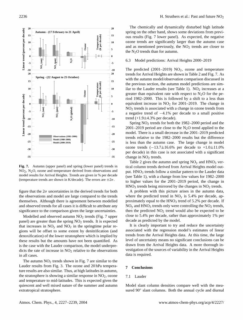
Fig. 7. Autumn (upper panel) and spring (lower panel) trends inNO2, N2O, ozone and temperature derived from observations andmodel results for Arrival Heights. Trends are given in % per decade(temperature trends are shown in K/decade). The errors are±2σ .

figure that the 2σ uncertainties in the derived trends for boththe observations and model are large compared to the trendsthemselves. Although there is agreement between modelledand observed trends for all cases it is difficult to attribute anysignificance to the comparison given the large uncertainties.

Modelled and observed autumn NO2 trends (Fig.7 upperpanel) are greater than the spring NO2 trends. It is expectedthat increases in NOy and NO2 in the springtime polar re-gions will be offset to some extent by denitrification (anddenoxification) of the lower stratosphere which is implied bythese results but the amounts have not been quantified. Asis the case with the Lauder comparison, the model underpre-dicts the rate of increase in NO2 relative to the observationsin all cases.

The autumn NO2 trends shown in Fig.7 are similar to theLauder results from Fig.3. The ozone and 20 hPa tempera-ture results are also similar. Thus, at high latitudes in autumn,the stratosphere is showing a similar response in NO2, ozoneand temperature to mid-latitudes. This is expected given thequiescent and well mixed nature of the summer and autumnextratropical stratosphere.

The chemically and dynamically disturbed high latitudespring on the other hand, shows some deviations from previ-ous results (Fig.7 lower panel). As expected, the negativeozone trends are significantly larger than the autumn caseand as mentioned previously, the NO2 trends are closer tothe N2O trends than for autumn.

6.3 Model predictions: Arrival Heights 2000–2019

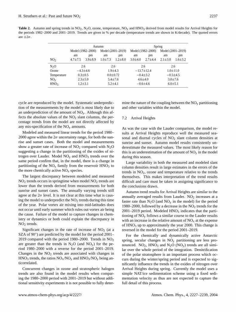
The predicted (2001–2019) NO2, ozone and temperaturetrends for Arrival Heights are shown in Table2 and Fig.7. Aswith the autumn model/observation comparison discussed inthe previous section, the autumn model predictions are sim-ilar to the Lauder results (see Table1). NO2 increases at agreater than equivalent rate with respect to N2O for the pe-riod 1982–2000. This is followed by a shift to a less thanequivalent increase in NO2 for 2001–2019. The change inNO2 trends is associated with a change in ozone trends froma negative trend of−4.1% per decade to a small positivetrend (+1.9±4.3% per decade).

Spring NO2 trends for both the 1982–2000 period and the2001–2019 period are close to the N2O trend applied to themodel. There is a small decrease in the 2001–2019 predictedtrends relative to the 1982–2000 results but the differenceis less than the autumn case. The large change in modelozone trends (−13.7±16.6% per decade to +1.0±11.0%per decade) in this case is not associated with a significantchange in NO2 trends.

Table2 gives the autumn and spring NOy and HNO3 ver-tical column trends derived from Arrival Heights model out-put. HNO3 trends follow a similar pattern to the Lauder data(see Table1), with a change from low values for 1982–2000to higher values for the 2001–2019 period, the change inHNO3 trends being mirrored by the changes in NO2 trends.

A problem with this picture arises in the autumn data,where the predicted trend in NOy is 5.4% per decade, ap-proximately equal to the HNO3 trend of 5.2% per decade. IfNOy and HNO3 trends only were controlling the NO2 trends,then the predicted NO2 trend would also be expected to beclose to 5.4% per decade, rather than approximately 1% perdecade as predicted by the model.

It is clearly important to try and reduce the uncertaintyassociated with the regression model’s estimates of lineartrends from the Arrival Heights data. At this time, the largelevel of uncertainty means no significant conclusions can bedrawn from the Arrival Heights data. A more thorough in-vestigation of the sources of variability in the Arrival Heightsdata is required.

7 Conclusions

7.1 Lauder

Model slant column densities compare well with the mea-sured 90◦ slant columns. Both the annual cycle and diurnal



Table 2. Autumn and spring trends in NO2, N2O, ozone, temperature, NOy and HNO3 derived from model results for Arrival Heights forthe periods 1982–2000 and 2001–2019. Trends are given in % per decade (temperature trends are shown in K/decade). The quoted errorsare±2σ .

Autumn SpringModel (1982–2000) Model (2001–2019) Model (1982–2000) Model (2001–2019)

am pm am pm am pm am pmNO2 4.7±7.5 3.9±8.9 1.0±7.3 1.2±8.0 3.0±4.0 2.7±4.4 2.1±3.0 1.6±3.2

N2O 2.6 2.6 2.6 2.6Ozone −4.3±4.6 1.9±4.3 −13.7±12.4 1.0±11.0Temperature 0.3±0.5 0.0±0.72 −0.4±3.2 −0.5±4.5NOy 2.3±5.0 5.4±7.6 4.6±4.0 3.0±7.6HNO3 1.2±3.1 5.2±4.1 −0.6±4.6 6.0±5.1

cycle are reproduced by the model. Systematic underpredic-tion of the measurements by the model is most likely due toan underprediction of the amount of NOy. Although this af-fects the absolute values of the NO2 slant columns, the per-centage trends from the model are not directly affected byany mis-specification of the NOy amounts.

Modeled and measured linear trends for the period 1980–2000 agree within the 2σ uncertainty range, for both the sun-rise and sunset cases. Both the model and measurementsshow a greater rate of increase of NO2 compared with N2Osuggesting a change in the partitioning of the oxides of ni-trogen over Lauder. Model NOy and HNO3 trends over thesame period confirm that, in the model, there is a change inpartitioning of the NOy family from the reservoir HNO3 tothe more chemically active NOx species.

The largest discrepancy between modeled and measuredNO2 trends occurs in springtime when model NO2 trends arelower than the trends derived from measurements for bothsunrise and sunset cases. The annually varying trends stillagree at the 2σ level. It is not clear at this time what is caus-ing the model to underpredict the NO2 trends during this timeof the year. Polar vortex air mixing into mid-latitudes doesnot occur until early summer which rules out vortex air beingthe cause. Failure of the model to capture changes in chem-istry or dynamics or both could explain the discrepancy inNO2 trends.

Significant changes in the rate of increase of NO2 (at aSZA of 90◦) are predicted by the model for the period 2001–2019 compared with the period 1980–2000. Trends in NO2are greater than the trends in N2O (and NOy) for the pe-riod 1980–2000 with a reverse for the period 2001–2019.Changes in the NO2 trends are associated with changes inHNO3 trends, the ratios NOx/NOy and HNO3/NOy being an-ticorrelated.

Concurrent changes in ozone and stratospheric halogentrends are also found in the model results when compar-ing the 1980–2000 period with 2001–2019 but without addi-tional sensitivity experiments it is not possible to fully deter-

mine the nature of the coupling between the NOy partitioningand other variables within the model.

7.2 Arrival Heights

As was the case with the Lauder comparison, the model re-sults at Arrival Heights reproduce well the measured sea-sonal and diurnal cycles of NO2 slant column densities atsunrise and sunset. Autumn model results consistently un-derestimate the measured values. The most likely reason forthis is an underestimation of the amount of NOy in the modelduring this season.

Large variability in both the measured and modeled slantcolumn densities result in large estimates in the errors of thetrends in NO2, ozone and temperature relative to the trendsthemselves. This makes interpretation of the trend resultsdifficult and care must be taken in assigning significance tothe conclusions drawn.

Autumn trend results for Arrival Heights are similar to theannually averaged results from Lauder. NO2 increases at afaster rate than N2O (and NOy in the model) for the period1980–2000, followed by a decrease in the NO2 trends for the2001–2019 period. Modeled HNO3 indicates that the parti-tioning of NOy follows a similar course to the Lauder resultswith an increase in the relative amount of NOx at the expenseof HNO3 up to approximately the year 2000. This change isreversed in the model for the period 2001–2019.

For the chemically and dynamically active Antarcticspring, secular changes in NOy partitioning are less pro-nounced. NO2, HNO3 and N2O (NOy) trends are all simi-lar over the whole period of the integration. Denitrificationof the polar stratosphere is an important process which oc-curs during the winter/spring period and is expected to sig-nificantly influence the trends in the oxides of nitrogen overArrival Heights during spring. Currently the model uses asimple NAT/ice sedimentation scheme using a fixed sedi-mentation velocity as thus are not expected to capture thefull detail of this process.



Results from both Lauder and Arrival Heights demonstratethat changes in NO2 slant column densities derived fromUMETRAC output follow the observed trends for the period1981–2000. This suggests processes influencing the nitrogenchemistry within the model are reasonably well represented.Interestingly, the model prediction of the trends in NO2 andHNO3 for the period 2001–2019 show a reversal comparedwith the period 1981–2000. NO2 trends are predicted to fallbelow the N2O trends, associated with an increase in theHNO3 trends indicating a shift in the partitioning of NOyaway from it’s active form at Lauder and Arrival Heights (au-tumn) over the coming two decades. Additional analysis ofthe model data is required to examine to what fraction of thechange in NO2 and HNO3 trends can be attributed to circu-lation changes and what fraction is associated with chemicalforcing.

Acknowledgements.The authors would like to thank G. Keys forhis work on the reanalysis of Arrival Heights measurements. TheNO2 measurements used in this publication were obtained as partof the Network for Detection of Stratospheric Change (NDSC) andis publicly available (seehttp://www.ndsc.ncep.noaa.gov). Thiswork was funded by the New Zealand Foundation of ResearchScience and Technology.

Edited by: J. Brandt

References

Ajtic, J., Connor, B., Lawerence, B., Bodeker, G., Hoppel, K.,Rosenfield, J., and Heuff, D.: Dilution of the Antarctic ozonehole into southern midlatitudes: 1998–2000, J. Geophys. Res.,accepted, 2004.

Austin, J.: On the explicit versus family solution of the fully diurnalphotochemical equations of the stratosphere, J. Geophys. Res.,96, 12 941–12 974, 1991.

Austin, J. and Butchart, N.: Coupled chemistry-climate model sim-ulations for the period 1980–2020: Ozone depletion and the startof the ozone recovery, Q. J. R. Meteorol. Soc., 129, 3225–3249,2003.

Bodeker, G., Boyd, I., and Matthews, W.: Trends and variability invertical ozone and temperature profiles measured by ozoneson-des as Lauder, New Zealand: 1986-1996, J. Geophys. Res., 103,28 661–28 681, 1998.

Bodeker, G., Scott, J., Kreher, K., and McKenzie, R.: Global ozonetrends in potential vorticity coordinates using TOMS and GOMEintercompared against the Dobson network: 1978–1998, J. Geo-phys. Res., 106, 23 029–23 042, 2001.

Brasseur, G. and Solomon, S.: Aeronomy of the middle atmosphere,D. Reidel Publishing Company, Dordrecht, The Netherlands, 2ndEdn., 1986.

Bucholtz, A.: Rayleigh-scattering calculations for the terrestrial at-mosphere, Appl. Opt., 34, 2765–2773, 1995.

Crutzen, P.: The influence of nitrogen oxides on the atmosphericozone content, Q. J. R. Meteorol. Soc., 96, 320–325, 1970.

Cullen, M. and Davies, T.: Conservative split-explicit integrationscheme with fourth-order horizontal advection, Q. J. R. Meteo-rol. Soc., 117, 993–1002, 1991.

DeMore, W., Sander, S., Golden, D., Hampson, R., Kurylo, M.,Howard, C., Ravishankara, A., Kolb, D., and Molina, M.: Chem-ical kinetics and photochemical data for use in stratospheric mod-elling, Tech. Rep. Evaluation number 12, Pasadena, Ca, 1997.

Fish, D., Roscoe, H., and Johnston, P.: Possible causes of strato-spheric NO2 trends observed at Lauder, New Zealand, Geophys.Res. Lett., 27, 3313–3316, 2000.

Grainger, J. and Ring, J.: Lunar luminescence and solar radiation,Space Res., 3, 989, 1963.

IPCC: IPCC, Climate Change 2001: The Scientific Basis, Contribu-tion of Working Group 1 to the Third Assessment Report of theIntergovernmental Panel on Climate Change, Tech. rep., Cam-bridge, UK, 2001.

Johnston, P. and McKenzie, R.: NO2 observations at 45◦ S duringthe decreasing phase of solar cycle 21, from 1980 to 1987, J.Geophys. Res., 94, 3473–3486, 1989.

Kalnay, E., Kanamitsu, M., Kistler, R., Collins, W., Deaven, D.,Gandin, L., Iredell, M., Saha, S., White, G., Woollen, J., Zhu, Y.,Leetmaa, A., Reynolds, R., M.Chelliah, Ebisuzaki, W., Higgins,W., Janowiak, J., Mo, K. C., Ropelewski, C., Wang, J., Jenne, R.,and Joseph, D.: The NCEP/NCAR 40-year reanalysis project,Bull. Am. Meteorol. Soc., 77, 437–471, 1996.

Keys, J. and Johnston, P.: Stratospheric NO2 and O3 in Antarc-tica: Dynamic and chemically controlled variations, Geophys.Res. Lett., 13, 1260–1263, 1986.

Keys, J. and Johnston, P.: Stratospheric NO2 column measurementsfor three Antarctic sites, Geophys. Res. Lett., 15, 898–900, 1988.

Liley, J., Johnston, P., McKenzie, R., Thomas, A., and Boyd, I.:Stratospheric NO2 variations from a long time series at Lauder,New Zealand, J. Geophys. Res., 105, 11 633–11 640, 2000.

McKenzie, R. and Johnston, P.: Springtime stratospheric NO2 inAntarctica, Geophys. Res. Lett., 11, 73–75, 1984.

McKenzie, R., Johnston, P., McElroy, C., Kerr, J., and Solomon,S.: Altitude distributions of stratospheric constitutuents fromground-based measurements at twilight, J. Geophys. Res., 96,15 499–15 511, 1991.

McLinden, C., Olsen, S., Prather, M., and Liley, J. B.: Understand-ing trends in stratospheric NOy and NO2, J. Geophys. Res., 106,27 787–27 793, 2001.

Minschwener, K., Salawitch, R., and McElroy, M.: Absorption ofsolar radiation by O2: Implications for O3 and lifetimes of N2O,CFCl3 and CF2Cl2, J. Geophys. Res., 98, 10 543–10 561, 1993.

Plumb, R. and Ko., M. K. W.: Interrelationships between mixingratios of long-lived stratospheric constituents, J. Geophys. Res.,99, 10 145–10 156, 1992.

Randel, W., Wu, F., Oltmans, S., Rosenlof, K., and Nedoluha, G.:Interannual cahnges in stratospheric water vapour and correla-tions with tropical tropopause temperatures, J. Atmos. Sci., 61,2 133–2 148, 2004.

Randeniya, L., Vohralik, P., Plumb., I., and Ryan, K. R.: Heteroge-neous BrONO2 hydrolysis: Effect on NO2 columns and ozone athigh latitudes in summer, J. Geophys. Res., 102, 23 543–23 557,1997.

Randeniya, L., Vohralik, P., and Plumb, I.: Stratosphericozone depletion at northern mid latitudes in the 21st cen-tury: The importance of future concentrations of greenhousegases nitrous oxide and methane, Geophys. Res. Lett., 29,doi:10.1029/2001GL014 295, 2002.


http://www.ndsc.ncep.noaa.gov


Rinsland, C., Weisenstein, D., Ko, M. K. W., Scott, C., Chiou, L.,Mahein, E., Zander, R., and Demoulin, P.: Post-Mount Pinatuboeruption ground-based measurements of HNO3, NO and NO2and their comparison with model calculations, J. Geophys. Res.,108, doi:10.1029/2002JD002 965, 2003.

Rodriguez, J., Ko, M. K. W., and Sze, N.-D.: Role of heterogeneousconversion of N2O5 on sulphate aerosols in global ozone losses,Nature, 352, 134–137, 1991.

Rosenlof, K., Oltmans, S., Kley, D., Russell, J., Chiou, E.-W., Chu,W., Johnson, D., Kelly, K., Michelsen, H., Nedoluha, G., Rems-berg, E., Toon, G., and McCormick, M.: Stratospheric watervapour increases over the past half-century, Geophys. Res. Lett.,28, 1195–1198, 2001.

Sander, S., Ravishankara, A., Friedl, R., DeMore, W., Golden, D.,Kolb, C., Kurylo, M., Molina, M., Hampson, R., Huie, R., andMoortgat, G.: Chemical kinetics and photochemical data for usein stratospheric modelling, Tech. Rep. Evaluation number 12:Update of key reactions, Pasadena, Ca, 2000.

Scaife, A., Butchart, N., Warner, C., Stainforth, D., Norton, W., andAustin, J.: Realistic quasi-biennial oscillations in a simulation ofthe global climate, Geophys. Res. Lett., 27, 3481–3484, 2000.

Schofield, R., Connor, B. J., Kreher, K., Johnston, P., and Rodgers,C.: The retrieval of profile and chemical information fromground-based UV-Visible spectroscopic measurements, J. Quan-titative Spectroscopy and Radiative Transfer, 86, 115–131, 2003.

Solomon, S., Schmeltekopf, A., and Saunders, R.: On the interpre-tation of zenith sky absorption measurements, J. Geophys. Res.,92, 8311–8319, 1987.

SPARC: 2000: SPARC assessment of upper tropospheric and strato-spheric water vapour, Tech. Rep. WMO-TD No. 1043, WCRPSeries Report No. 113, SPARC Report No. 2, Berrieres le Buis-son Cedex,http://www.aero.jussieu.fr/∼sparc/WAVASFINAL000206/WWWwavas/WavasComplet.pdf, 2000.

Warner, C. and McIntyre, M.: Toward an ultra simple spectral grav-ity wave parameterization for general circulation models, EarthPlanets Space, 51, 475–484, 1999.

WMO: Scientific Assessment of Ozone Depletion: 1991, WMOGlobal Ozone Research and Monitoring Project, Tech. Rep. Re-port No. 25, Geneva, Switzerland, 1991.



Zander, R., Ehhalt, D., Rinsland, C., Schmidt, U., Mahieu, E.,Rudolph, J., Demoulin, P., Roland, G., Delbouille, L., andSauval, A.: Secular trend and seasonal variability of the columnabundance of N2O above the Jungfraujoch station determinedfrom IR spectra, J. Geophys. Res., 99, 16 745–16 756, 1994.


http://www.aero.jussieu.fr/~sparc/WAVASFINAL_000206/WWW_wavas/WavasComplet.pdf

http://www.aero.jussieu.fr/~sparc/WAVASFINAL_000206/WWW_wavas/WavasComplet.pdf

Documents

and Physics Chemistry Past and future simulations of NO ... · Chemistry and Physics Past and future simulations of NO2 from a coupled chemistry-climate model in comparison with observations