•and Pahlavi University~ Shiraz, Iran .

INFORMATION MATRIX FOR A11IXTURE

OF Two NoRf.W.. DISTRIBUTIONS

Javad Behboodian*Department of Statistics

University of North Carolina at Chapel Hitz

Institute of Statistics Mimeo Series No. 747

ApJc1.i.., 1971

of a mixture

• INFORMc\TION f1ATRIX FOR A NIXTURE OF T~'IO f'hRMAL DISTRIBUTIONS

Javad BehboodianUnivepsity of Nopth CaPo Una at Chapel. BiU

and PahZaoi Univepsity" Shipa2" Ipan

(-\BSTRACT

This paper presents a numerical method for computation of the Fisher in-

formation matrix about the five parameters ~1' ~2' p, °1 2, 022

of two normal distributions. It is shown, by using a simple transformation

which reduces the number of parameters from five to three, that the computation

of the whole information matrix leads to the numerical evaluation of a parti-

cu1ar integral. The Hermite-Gauss quadratuse formula, the Romberg's algorithm,

a power series, and Taylor's expansion are applied for the evaluation of this

integral and the results are compared with each other.

A short table has been provided from which the approximate information

matrix can be obtained in practice.

1. INTRODUCTION

Consider

f(x) = pf1

(x) + qf2

(x) (1.1)

where fj(x) is a normal density with parameters ~j and 0j2, j = 1,2,

with 0 < p < 1 and q = 1-p. The function f(x) is the probability density

function of a mixture of two normal distributions with mixing proportions p

and q. The point estimation of the parameters of this distribution has re-

cent1y received some attention in the literature [1, 3, 4, 6]. However, due to

2

the complexity of the problem, there is no simple way to measure the precision

~ of the estimators obtained by different methods or to consider optimal sample

size for specified precision. A convenient statistical measure which can be

used for assessing the sample size before experiment and evaluating the approx­

imate precision after estimation is the Fisher information, whose properties

are well-known.

This paper presents a numerical method for computation of the Fisher in­

formation matrix about the five parameters ~1' ~2' p, °1 2 , 022 of a mixture

of two normal distributions, which can even be extended to finite mixtures of

more than two normal distributions. The first work related to this paper is

by Hill [8], who gives a general power series for computing the Fisher infor­

mation of the proportion p in a mixture of two densities. In particular, he

considers the case of exponential mixture and normal mixture with equal vari­

ances in more detail. The information matrix is also computed by the author

in [2] for the special case of a normal mixture with equal variances.

Our attempt here is to show that the computation of the whole information

matrix leads to the numerical evaluation of a particular integral, by using a

simple transformation which reduces the number of parameters from five to

three positive ones. The Hermite-Gauss quadrature formula, the Romberg's

algorithm, a power series, and Taylor's expansion are applied for the evalu­

ation of this integral and the results are compared with each other. A short

table has been provided from which the information matrix can be easily com­

puted in practice.

3

2. INFORMATION rv1ATRIX

Let X be a random variable with the probability density function f(x,8)

depending on an h-dimensional parameter 8 = (61

,82

, ••• ,6h). The information

matrix that we shall use is that of Fisher, namely, the symmetric positive def-

inite hxh matrix 1(6) = I II(6s ,8 t )1 I with

I(6s

,6t

) = E ~ tog f(x,6) • a tog f(X26~a8 ae

t'

- ss,t = l,2, ••• ,h, (2.1)

where the expectation is taken with respect to the density f(x,e), and it is

assumed that all the derivatives and expectations in question exist.

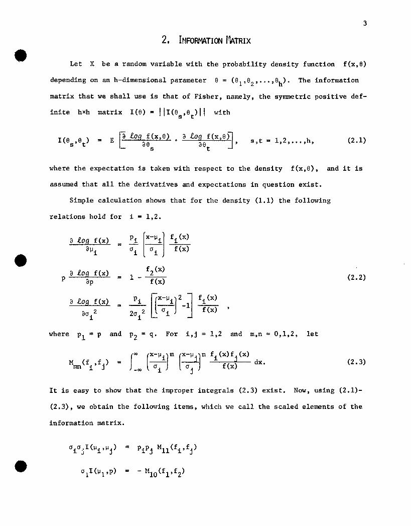
Simple calculation shows that for the density (1.1) the following

relations hold for i = 1,2.

a tog f (x) Pi [X::iJ £i (x)=all i °i £(x)

a tog f (x)1 -

f2

(x)p =ap £(x)

a tog f (x) Pi l-"ir ~fi(x)

= -- ---1ao 2 20/ _ °i f(x)

i

(2.2)

where and For i,j = 1,2 and m,n = 0,1,2, let

M (f ,f.)ron i J · C[x::r [~r (2.3)

It is easy to show that the improper integrals (2.3) exist. Now, using (2.1)-

(2.3), we obtain the following items, which we call the scaled elements of the

information matrix.

=

I(p,p)

0/1 (p ,°12

)

O/I(p,o/)

° 20 21(0 2 0 2)1 2 l' 2

= MOl (f1' f 2)

PPi= --2-- [M12(fl,fi)-MlO(fl,fi)]

Piq

= --2-- [M2l(fi,f2)-MOl(fi,f2)]

1= pq [1-MOO (fl ,f2)]

1= 2 [MOO(fl,f2)-M20(fl,f2)]1• 2 [M02(fl,f2)-MOO(fl,f2)]

= ~ [MOO(fl,f2)-M20(fl,f2)-M02(fl,f2)+M22(fl,f2)]

Pi2

= -r- [MOO(fi,fi)-2Mll(fi,fi)+M22(fi,fi)]·

4

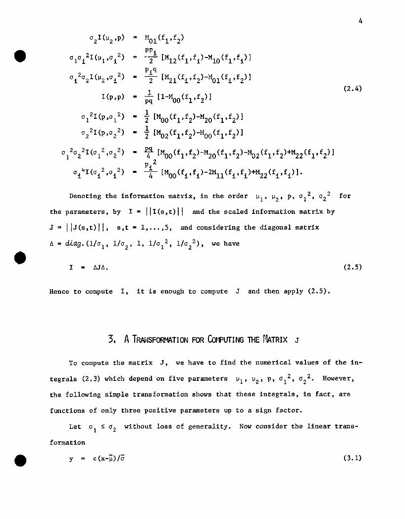
(2.4)

Denoting the information matrix, in the order ~1' ~2' p, 0 12 , 022 for

the parameters, by I = I II(s,t)1 I and the scaled information matrix by

J = I IJ(s,t)1 I, s,t = 1, ••• ,5, and considering the diagonal matrix

~ = diag.(l/ol' 1/02' 1, 1/°1 2 , 1/022), we have

• I = M~.

Hence to compute I, it is enough to compute J and then apply (2.5).

3. ATRANSFORMATION FOR CavpUTING THE r~TRIX J

(2.5)

To compute the matrix J, we have to find the numerical values of the in-

tegrals (2.3) which depend on five parameters However,

the following simple transformation shows that these integrals, in fact, are

functions of only three positive parameters up to a sign factor.

Let 01 ~ O2 without loss of generality. Now consider the linear trans­

formation

(3.1)

5

assuming that E = 1 for ~1 S ~2 and E = -1 for ~1 > ~2' where

=

Take also

-o = 10 10 2 , (3.2)

(3.3)

where D ~ 0 and 0 < r S 1. One can easily show that the transformation

(3.1) sends the density function (1.1) to the density function

with the conventions Dl = -D, D2 = D, r l = r, and r 2 = l/r. Thus, by using

the transformation (3.1), the normal mixture (1.1) with five parameters is•

where, for i = 1,2,

=

(3.4)

(3.5)

reduced to (3.4), say, the standard normal mixture with three positive param-

eters D, p, r.

It is obvious that under the linear transformation (3.1) the formula (2.3)

becomes

= (3.6)

with

= (3.7)

As the formulae (2.4) show, the sign factor m+nE only affects the elements

I(~i'P) and I(~i,Oj2), for i,j = 1,2, when ~1 > ~2' Thus, to make the

tabulation of the results easier, we can assume, as well, that ~1 S ~2 and

eliminate m+ne: ; whenever ~l > ~2' we just give a minus sign to the above

6

mentioned elements which depend on ~l and ~2 through D = 1~2-~11/2a.

4. HERMITE-GAusS QuADRATURE NJD RoM3ERG'S ALGORITHt1

FOR CoWUTATION OF Gmn (gi ,gj)

The Hermite-Gauss quadrature formula for a convergent integral of the form

fa> e-Z2

leG) = G(z)dz-a>

is

NleG) = k~l wk G(zk) + ~(G),

(4.1)

(4.2)

where zk and wk ' which are referred to respectively as nodes and weights,

can be determined through some appropriate Hermite polynomials and they are

,Nalready known and tabulated [7 s 9]. The summation lk=l WkG(zk)

leG) with the remainder

~(G) = N! lIT G(2N) (z)/2N (2N)1 ,

approximates

(4.3)

where z is a real number. In general, the size of ~(G) depends on the be­

havior of the derivatives of G(z) over (-a>,a», and it cannot be easily

estimated. To guarantee a sufficiently small error, it is desirable that these

derivatives remain bounded with a small supremum over (-a>,a».

Now we show that the integral (3.7), by introducing the suitable factor

exp(-ry2/4), can be put in the form (4.1) with a bounded function G(z) and

bounded derivatives G(N)(z). For this purpose we write

gi(y)gj(y)/g(y) =

2 i -1-1exp(-ry /4)/ [pgl (y)gi (y)gj (y)

(4.4)-1 -1 2+ Qg2(y)gi (y)gj (y)]oexp(-ry /4),

7

and we use the transformation Z = ylr/2 to obtain

= (4.5)

where simple calculation shows that for m,n = 0,1,2 and i,j = 1,2,

cmnij-(m+n)/2 -1/2 -1/2 ~2/= r r i r j vZ/TI

= (2Z-Dilr)m(2Z-Dj;r)n~ [pexPQijl(z) + qrexPQij2(z)]

2= Aijk Z + Bijk Z + Cijk (4.6)

Aijk = 2(1/ri + l/rj - l/rk - r/2)/r

= -2(Di /ri + Dj/rj - Dk/rk)/Ir

222= (Di /ri + Dj /rj - Dk /rk)/2.

The relations (4.6) show that the function Gmnij(z) and its derivatives

are bounded on (-~,~). So, the remainder (4.3) for this function goes to

zero as N becomes large, and the numerical value of Gmn(gi,gj) can be

approximated by L~=l Wt Gmnij(Zt). However, it is noticed that when r is

very small the contribution of Gmnij(Zt) to the summation, for large values

of Zt' may be very trivial due to the largeness of the exponential terms

exp Qijk(Zt). This causes a slow convergence and sometimes it leads to poor

approximations. To obtain more accurate results, we apply the Romberg's

algorithm, which is known [10], for the numerical evaluation of (4.5) when r

is small. This can be done by breaking the range of integration and using some

appropriate transformations to change the integral (4.5) into sum of three

integrals on the interval (0,1).

The function Gmnij(z) is so complicated that we cannot find an estimate

for the remainder term though the computation shows that our results are

accurate at least up to four decimal points. To have a better check on the

8

results, in the next section we introduce some power series for the numerical

5. SoME P(),lER SERIES ExpmSIONS FOR lliE CortPUTATION OF

In this section, we mention briefly some power series expansions for the

evaluation of the integral (3.7), and we compare some of the results with the

above approximations.

First we use a series expansion similar to the one employed by Hill [8]

for the computation of I(p,p), in the special case that 01

2 = 0 22 • We ob­

serve, from (3.4)-(3.5), that

gi(y)gj(y)

g(y)

where

(5.1)

with

i = 1,2.

(5.2)

(5.3)

Now, it is easy to show that ph1 (y)/qrh2(y) < 1 if Y is in the interval

(-~ u l ) or (u2'~)' with u 1 < u 2 ' and qrh2(y)/ph(y) < 1 if y is in the

interval (u l ,u2), where u l and u2 are the real roots of the equation

(5.4)

if such real roots exist. When the roots are imaginary or equal,

ph1

(y)/qrh2(y) < 1 for all y. If r = 1, then ph1(y)/qrh2(y) < 1 for y

9

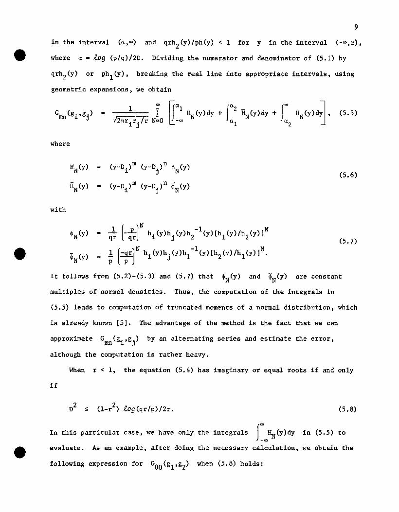
in the interval (a,ro) and qrh2(y)/ph(y) < 1 for y in the interval (-ro,a),

where a· log (p/q)/2D. Dividing the numerator and denominator of (5.1) by

qrh2(y) or phl(y), breaking the real line into appropriate intervals, using

geometric expansions, we obtain

where

= (5.5)

~(y)

~(y)

with

=

=

m n(y-Di ) (y-Dj

) ~N(Y)

m n -(y-Di ) (y-Dj ) ~N(Y)

(5.6)

(5.7)

It follows from (5.2)-(5.3) and (5.7) that ~N(Y) and ~N(Y) are constant

multiples of normal densities. Thus, the computation of the integrals in

(5.5) leads to computation of truncated moments of a normal distribution, which

is already known [5]. The advantage of the method is the fact that we can

approximate Grnn(gi,gj) by an alternating series and estimate the error,

although the computation is rather heavy.

~fuen r < 1, the equation (5.4) has imaginary or equal roots if and only

if

(5.8)

In this particular case, we have only the integrals f~ro~(Y)dY in (5.5) to

evaluate. As an example, after doing the necessary calculation, we obtain the

following expression for GOO (gl,g2) when (5.8) holds:

00

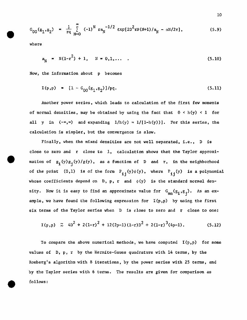
Jl \ ( N -1/2 2 /= L -1) r~ exp[2D rN(N+l) a. - aN/2r],rq N=O ~

10

(5.9)

where

N = 0,1, ••• (5.10)

Now, the information about p becomes

(5.11)

Another power series, which leads to calculation of the first few moments

of normal densities, may be obtained by using the fact that 0 < h(y) < 1 for

all y in (-00,00) and expanding l/h(y) = l/[l-h(y»]. For this series, the

calculation is simpler, but the convergence is slow.

Finally, when the mixed densities are not well separated, Le., D is

close to zero and r close to 1, calculation shows that the Taylor approxi-

mation of gi(y)gj(y)/g(y), as a function of D and r, in the neighborhood

of the point (0,1) is of the form Pij (y)<P (y) , where Pij(y) is a polynomial

whose coefficients depend on D, p, r and <I>(Y) is the standard normal den-

sity. Now it is easy to find an approximate value for Gmn(gi,gj). As an ex­

ample, we have found the following expression for I(p,p) by using the first

six terms of the Taylor series when D is close to zero and r close to one:

I(p,p) 2 2 2 34D + 2(1-r) + l2(2p-l)(1-r)D + 2(1-r) (4p-l). (5.12)

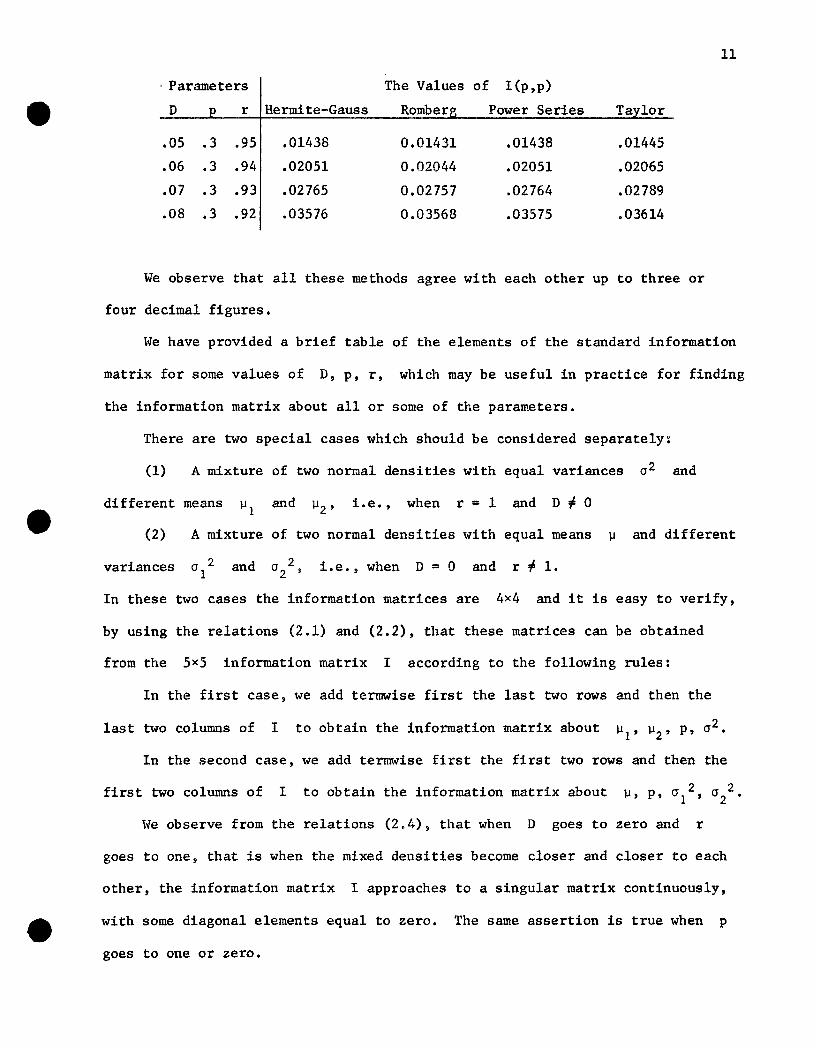
To compare the above numerical methods, we have computed I(p,p) for some

values of D, p, r by the Hermite-Gauss quadrature with 14 terms, by the

Romberg's algorithm with 8 iterations, by the power series with 25 terms, and

by the Taylor series with 6 terms. The results are given for comparison as

follows:

11

. Parameters The Values of I(p,p)

D r Hermite-Gauss Romber Power Series Ta lor

.05 .3 .95 .01438 0.01431 .01438 .01445

.06 .3 .94 .02051 0.02044 .02051 .02065

.07 .3 .93 .02765 0.02757 .02764 .02789

.08 .3 .92 .03576 0.03568 .03575 .03614

We observe that all these methods agree with each other up to three or

four decimal figures.

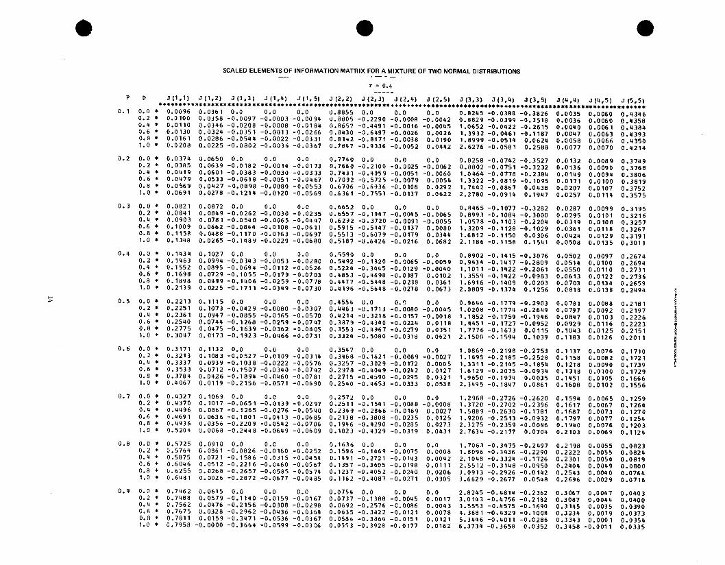
We have provided a brief table of the elements of the standard information

matrix for some values of D, p, r, which may be useful in practice for finding

the information matrix about all or some of the parameters.

There are two special cases which should be considered separately:

(1) A mixture of two normal densities with equal variances 0 2 and

different means and J.l 2 ' i.e., when r = 1 and D ~ 0

(2) A mixture of two normal densities with equal means J.l and different

variances o 21

and 02

2 , 1.e., when D = 0 and r ~ 1.

In these two cases the information matrices are 4x4 and it is easy to verify,

by using the relations (2.1) and (2.2), that these matrices can be obtained

from the 5x5 information matrix I according to the following rules:

In the first case, we add termwise first the last two rows and then the

last two columns of I to obtain the information matrix about J.l1

' J.l2

' p, 0 2 •

In the second case, we add termwise first the first two rows and then the

first two columns of I to obtain the information matrix about J.l, p, 01

2 , 02

2 •

lie observe from the relations (2.4), that when D goes to zero and r

goes to one, that is when the mixed densities become closer and closer to each

other, the information matrix I approaches to a singular matrix continuously,

with some diagonal elements equal to zero. The same assertion is true when p

goes to one or zero.

It is known that for a sample of size, say N,

12

is the asymptotic

covariance matrix of the maximum likelihood estimates of the parameters, and

the diagonal elements of I-lIN are the variances of the asymptotic distri-

bution of these estimates. Combining this fact with the above assertion, we

conclude that for estimating the parameters of a mixture of two normal distri-

butions with mixed densities, which are not well-separated, or with a mixing

proportion close to zero we need a huge sample, and the estimation may be im-

possible.

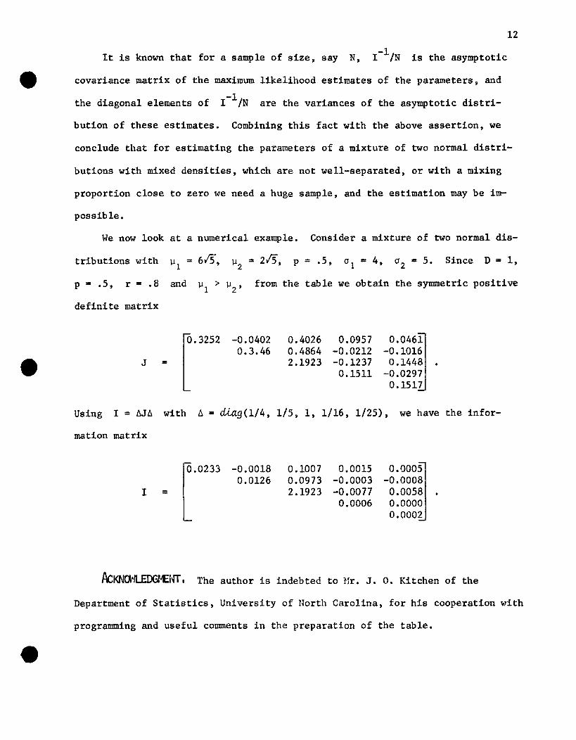
We now look at a numerical example. Consider a mixture of two normal dis-

tributions with ~1 = 615, ~2 = 215, p = .5, 01 = 4, 02 = 5. Since D = 1,

p = .5, r = .8 and ~1 > ~2' from the table we obtain the symmetric positive

definite matrix

J =

0.3252 -0.04020.3.46

0.40260.48642.1923

0.0957-0.0212-0.1237

0.1511

0.0461-0.1016

0.1448-0.0297

0.1517

Using I = 6J6 with 6 = diag(1/4, lIS, 1, 1/16, 1/25), we have the infor-

mation matrix

I =

0.0233 -0.00180.0126

0.10070.09732.1923

0.0015-0.0003-0.0077

0.0006

0.0005-0.0008

0.00580.00000.0002

AcKNorl~18NT, The author is indebted to ~1r. J. O. Kitchen of the

Department of Statistics, University of North Carolina, for his cooperation with

programming and useful comments in the preparation of the table.

e - eSCALED ELEMENTS OF INFORMATION MATRIX FOR A MIXTURE OF TWO NORMAL DISTRIBUTIONS

r • 0.2---_.

p D JIl,l) J (1,2) J (1,3) J (1,ij) J (1, 5) J (2,2) J (2,3) J (2,ij) J (2,5) J (3,3) J ll,ij) J (3,5) J (4,ij) J (4,5) J (5,5)•••••••***••••••••••••••••••••••••••••••••••••••••••••••••••••••••••••••••••••••••••••••••••••••••••••••••••••••••••••••0.1 0.0 • 0.0157 0.0169 0.0 0.0 0.0 0.8963 0.0 0.0 0.0 2.1540 -0.0650 -0.3843 0.0055 -0.0010 0.43280.2 • 0.0159 0.0167 -0.0049 -0.0002 -0.0032 0.8940 -0.1426 -0.0010 -0.0056 2.1925 -0.0660 -0.3700 0.0056 -0.0010 0.4338

0.4 • 0.0165 0.0164 -0.0101 -0.0004 -0.0063 0.8872 -0.2814 -0.0021 -0.0099 2.3079 -0.0677 -0.3276 0.0058 -0.0008 0.43650.6 • 0.0176 0.0157 -0.0159 -0.0006 -0.0093 0.8763 -0.4124 -0.0033 -0.0109 2.5073 -0.0706 -0.2591 0.0062 -0.0004 0.44020.8 • 0.0192 0.0147 -0.0224 -0.0009 -0.0120 0.8620 -0.5309 -0.0046 -0.0090 2.7972 -0.0747 -0.1678 0.0067 0.0001 0.44351.0 • 0.0214 0.0133 -0.0301 -0.0012 -0.0142 0.8ij53 -0.6322 -0.0062 -0.0028 3.1823 -0.0799 -0.0593 0.0075 0.0009 0.4451

0.2 0.0 • 0.0558 O. 0288 0.0 0.0 0.0 0.7939 0.0 0.0 0.0 1.9493 -0.1064 -0.3261 0.0192 -0.0049 0.37460.2 • 0.0564 0.0285 -0.0080 -0.0007 -0.0057 0.7905 -0.1206 -0.0029 -0.0079 1.9785 -0.1069 -0.3131 0.0194 -0.0047 0.37610.4 • 0.0582 0.0274 -0.0162 -0.0014 -0.0112 0.7806 -0.2362 -0.0059 -0.0141 2.0652 -0.1083 -0.2754 0.0200 -0.0041 0.38030.6 • 0.0613 0.0256 -0.0250 -0.0021 -0.0162 0.7650 -0.3417 -0.0091 -0.0155 2.2130 -0.1106 -0.2153 0.0211 -0.0030 0.38590.8 • 0.0656 0.0230 -0.0342 -0.0031 -0.0203 0.7452 -0.4319 -0.0124 -0.0122 2.4177 -0.1134 -0.1377 0.0226 -0.0014 0.39101.0 • 0.0714 0.0195 -0.0437 -0.0042 -0.0234 0.7232 -0.5024 -0.0158 -0.0031 2.6784 -0.1163 -0.0489 0.0246 0.0008 0.3948

0.3 0.0 • 0.1145 0.0371 0.0 0.0 0.0 0.6923 0.0 0.0 0.0 1.8633 -0.1373 -0.2867 0.0392 -0.0094 0.32100.2 • 0.1155 0.0359 -0.0102 -0.0014 -0.0075 0.6884 -0.1059 -0.0049 -0.0090 1.8879 -0.1375 -0.2749 0.0395 -0.0090 0.32280.4 • 0.1185 0.0348 -0.0206 -0.0028 -0.0147 0.6772 -0.2064 -0.0098 -0.0157 1.9601 -0.1380 -0.2407 0.0406 -0.0079 0.32760.6 • 0.1235 0.0318 -0.0311 -0.0043 -0.0210 0.6598 -0.2958 -0.0148 -0.0171 2.0816 -0.1389 -0.1869 0.0424 -0.0060 0.33400.8 • 0.1305 0.0276 -0.0419 -0.0061 -0.0260 0.6383 -0.3697 -0.0197 -0.0131 2.2462 -0.1396 -0.1187 0.0450 -0.0032 0.33981.0 • 0.1395 0.0223 -0.0523 -0.0081 -0.0293 0.6150 -0.4238 -0.0246 -0.0028 2.4499 -0.1396 -0.0426 0.0484 0.0003 0.3437

0.4 0.0 • 0.1887 0.0423 0.0 0.0 0.0 0.5913 0.0 0.0 0.0 1.8657 -0.1641 -0.2585 0.0650 -0.0135 0.27040.2 • 0.1900 0.0415 -0.0122 -0.0022 -0.0088 0.5874 -0.0940 -0.0068 -0.0091 1.8874 -0.1639 -0.2477 0.0655 -0.0129 0.27220.4 • 0.1941 0.0391 -0.0244 -0.0045 -0.0170 0.5760 -0.1851 -0.0131 -0.0153 1.9533 -0.1635 -0.2162 0.0671 -0.0113 0.27710.6 • 0.2007 0.0352 -0.0364 -0.0069 -0.0241 0.5586 -0.2638 -0.0196 -0.0169 2.0618 -0.1627 -0.1671 0.0697 -0.0086 0.28360.8 • 0.20'19 0.0298 -0.0481 -0.0095 -0.0294 0.5373 -0.3270 -0.0257 -0.0127 2.2066 -0.160'1 -0.1058 0.0734 -0.004'1 0.29011.0 • 0.2215 0.0230 -0.0590 -0.0123 -0.0326 0.5149 -0.3711 -0.0314 -0.0023 2.3827 -0.1579 -0.0385 0.0782 -0.0004 0.2932

~....0.5 0.0 • 0.2769 0.0446 0.0 0.0 0.0 0.4909 0.0 0.0 0.0 1.9560 -0.1906 -0.2377 0.0970 -0.0168 0.2218 •...,

I0.2 • 0.2783 0.0437 -0.0142 -0.0031 -0.0095 0.4872 -0.0876 -0.0080 -0.0085 1.9771 -0.1900 -0.2275 0.0978 -0.0161 0.22350.4 • 0.2833 0.0408 -0.0284 -0.0063 -0.0182 0.4764 -0.1695 -0.0156 -0.0142 2.0420 -0.1886 -0.1981 0.0997 -0.0140 0.22820.6 • 0.2916 0.0362 -0.0419 -0.0095 -0.0256 0.4602 -0.2342 -0.0238 -0.0156 2.1456 -0.1858 -0.1528 0.1029 -0.0108 0.2347 80.8 • 0.3019 0.0299 -0.0542 -0.0130 -0.0309 0.4406 -0.2962 -0.0299 -0.0114 2.2834 -0.1816 -0.0966 0.1079 -0.0063 0.2402 ~

i1. 0 • 0.3153 0.0223 -0.0654 -0.0165 -0.0337 0.4207 -0.3338 -0.0360 -0.0017 2.4488 -0.1756 -0.0357 0.1140 -0.0010 0.2428 i.0.6 0.0 • 0.3789 0.0442 0.0 0.0 0.0 0.3910 0.0 0.0 0.0 2.1629 -0.2201 -0.2220 0.1361 -0. 0188 0.1749 i0.2 • 0.3807 0.0432 -0.0163 -0.0042 -0.0095 0.3877 -0.0819 -0.0086 -0.0074 2.1846 -0.2190 -0.2125 0.1369 -0.0180 0.1764~0.4 • 0.3859 0.0400 -0.0322 -0.0080 -0.0182 0.3782 -0.1579 -0.0170 -0.0123 2.2525 -0.2163 -0.1848 0.1394 -0.0157 0.1808

0.6 • 0.3944 0.0350 -0.0475 -0.0121 -0.025ij 0.3640 -0.2232 -0.0248 -0.0134 2.3604 -0.2116 -0.1423 0.1435 -0.0121 0.18620.8 • 0.4059 0.0284 -0.0609 -0.0162 -0.0304 0.3470 -0.2736 -0.0319 -0.0096 2.5023 -0.2046 -0.0900 0.1492 -0.0073 0.19101. 0 • 0.4200 0.0204 -0.0726 -0.0202 -0.0328 0.3299 -0.3065 -0.0379 -0.0011 2.6711 -0.1955 -0.0339 0.1564 -0.0016 0.1932

0.7 0.0 • 0.4954 0.0409 0.0 0.0 0.0 0.2917 0.0 0.0 0.0 2.5689 -0.2569 -0.2108 0.1841 -0.0193 0.12950.2 • 0.4972 0.0398 -0.0190 -0.0048 -0.0089 0.2890 -0.0777 -0.0086 -0.0059 2.5949 -0.2554 -0.2016 0.1850 -0.0185 0.13070.4 • 0.5024 0.0367 -0.0374 -0.0095 -0.0170 0.2813 -0.1495 -0.0170 -0.0098 2.6728 -0.2511 -0.1751 0.1878 -0.0161 0.13410.6 • 0.5109 0.0317 -0.0575 -0.0141 -0.0239 0.2697 -0.2106 -0.0247 -0.0106 2.7963 -0.2439 -0.1348 0.1924 -0.0124 0.13840.8 • 0.5222 0.0251 -0.0694 -0.0187 -0.0280 0.2562 -0.2572 -0.0314 -0.0074 2.9578 -0.2338 -0.0855 0.1988 -0.0076 0.14211.0 • 0.5360 0.0174 -0.0818 -0.0230 -0.0298 0.2425 -0.2868 -0.0369 -0.0005 3.1481 -0.2209 -0.0329 0.2068 -0.0021 0.1439

0.8 0.0 • 0.6287 0.0343 0.0 0.0 0.0 0.1931 0.0 0.0 0.0 3.4378 -0.3103 -0.2036 0.2446 -0.0176 0.08500.2 • 0.6303 0.0333 -0.0230 -0.0052 -0.0076 0.1904 -0.0749 -0.0078 -0.0041 3.4731 -0.3082 -0.1947 0.2456 -0.0169 0.08630.4 • 0.6350 0.0304 -0.0451 -0.0103 -0.0144 0.1856 -0.1440 -0.0152 -0.0069 3.5534 -0.2999 -0.1710 0.2485 -0.0146 0.08820.6 • 0.6426 0.0259 -0.0649 -0.0152 -0.0198 0.1774 -0.2025 -0.0220 -0.0073 3.7402 -0.2912 -0.1303 0.2534 -0.0114 0.09120.8 • 0.6527 0.0201 -0.0819 -0.0198 -0.0232 0.1677 -0.2463 -0.0277 -0.0050 3.9549 -0.2768 -0.0829 0.2600 -0.0072 0.09391. a • 0.6648 0.0134 -0.0952 -0.0240 -0.0245 0.1581 -0.2737 -0.0323 0.0001 4.2045 -0.2590 -0.0329 0.2682 -0.0023 0.0951

0.9 0.0 • 0.7852 0.0230 0.0 0.0 0.0 0.0954 0.0 0.0 0.0 6.0560 -0.4104 -0.2019 0.3270 -0.0128 0.04180.2 • 0.7863 0.0222 -0.0303 -0.0049 -0.0051 0.0943 -0.0743 -0.0056 -0.0021 6.1216 -0.4070 -0.1932 0.3279 -0.0123 0.04220.4 • 0.7897 0.0202 -0.0590 -0.0096 -0.0097 0.0914 -0.1427 -0.0109 -0.0035 6.3144 -0.3970 -0.1679 0.3306 -0.0108 0.04340.6 • 0.7951 0.0169 -0.0845 -0.0140 -0.0133 0.0869 -0.2001 -0.0156 -0.0037 6.6170 -0.3805 -0.1298 0.3349 -0.0084 0.04490.8 • 0.8022 0.0127 -0.1056 -0.0180 -0.0154 0.0818 -0.2428 -0.0195 -0.0023 7.0128 -0.3587 -0.0834 0.3408 -0.0054 0.04631. 0 • 0.8107 0.0081 -0.1211 -0.0213 -0.0160 0.0767 -0.2689 -0.0225 0.0004 7.4696 -0.3322 -0.0346 0.3479 -0.0021 0.0469

e - eSCALED ELEMENTS OF INFORMATION MATRIX FOR A MIXTURE OF TWO NORMAL DISTRIBUTIONS

1-----

r = 0.4-----

p 0 J (1 ,1) J (1,2) J (1,3) J (1,4) J (1, 5) J (2,2) J (2,3) J (2,4) J (2,5) J (3,3) J(3,4) J (J. 5) J (4,4) J (4,5) J (5,5)••••••••••••••••••••••••••••••••••••••••••••••••••••••••••••••••••••••••••••••••••••••••••••••••••••••••••••••••••••••••O. 1 O. a * O. 0096 0.0361 0.0 0.0 0.0 0.8855 0.0 0.0 0.0 0.8245 -0.0388 -0.3826 0.0035 0.0060 0.4346

0.2 * 0.0100 0.0358 -0.0097 -0.0003 -0.0094 0.8805 -0.2290 -0.0008 -0.0042 0.8829 -0.0399 -0.3518 0.0036 0.0060 0.43580.4 * 0.0110 0.0346 -0.0208 -0.0008 -0.0184 0.8657 -0.4491 -0.0016 -0.0045 1.0652 -0.0422 -0.2615 0.0 040 0.0061 0.43840.6 * 0.0 130 0.0324 -0.0351 -0.0013 -0.0266 0.8430 -0.6497 -0.0026 0.0026 1.3932 -0.0461 -0.1187 0.0041 0.0063 0.43930.8 * 0.0161 0.0286 -0.0544 -0.0022 -0.0331 0.8142 -0.8111 -0.0038 0.0190 1. 8999 -0.0514 0.06211 0.0058 0.0066 0.43501.0 * 0.0208 0.0225 -0.0802 -0.0036 -0.0367 0.1841 -0.9336 -0.0052 0.0442 2.6216 -0.0581 0.2588 0.0011 O. 0070 0.42111

0.2 o. a * 0.0314 0.0650 0.0 0.0 0.0 0.1140 0.0 0.0 0.0 0.8258 -0.0142 -0.3527 0.0 132 0.0089 0.37490.2 * 0.0385 0.0639 -0.0182 -0.0014 -0.0113 0.1660 -0.2100 -0.0025 -0.0062 0.8802 -0.0751 -0.3232 0.0136 0.0090 0.37680.4 * 0.0419 0.0601 -0.0383 -0.0030 -0.0333 0.1431 -0.4059 -0.0051 -0.0060 1.0464 -0.0778 -0.2384 0.0149 0.0094 0.38060.6 * 0.0419 0.0533 -0.0618 ~0.0051 -0.0461 0.1092 -0.5125 -0.0019 0.0054 1.3322 -0.0819 -0.1095 0.0111 0.0100 0.38190.8 * 0.0569 0.0427 -0.0898 -0.0080 -0.0553 0.6706 -0.6936 -0.0108 0.0292 1.1442-0.0861 0.0438 0.0201 0.0101 0.37521.0 * 0.0691 0.0278 -0.1214 -0.0120 -0.0569 0.6361 -0.1553 -0.0131 0.0622 2.2780 -0.0914 0.19111 0.0251 0.0114 0.3515

0.3 0.0 * 0.0821 0.0812 0.0 0.0 0.0 0.6652 0.0 0.0 0.0 0.8465 -0.1071 -0.3282 0.0281 0.0099 0.31950.2 * 0.0841 0.0849 -0.0262 -0.0030 -0.0235 0.6551 -0.1941 -0.0045 -0.0065 0.8993 -0.1084 -0.3000 0.0295 0.0101 0.32160.4 * 0.0903 0.0781 -0.0540 -0.0065 -0.0441 0.6292 -0.3120 -0.0091 -0.0055 1.0518 -0.1103 -0.2204 0.0319 0.0108 0.32570.6 * 0.1009 0.0662 -0.0844 -0.0108 -0.0611 0.5915 -0.5141 -0.0137 0.0080 1.3209 -0.1128 -0.1029 0.0361 0.0118 0.32610.8 * 0.1158 0.0488 -0.1110 -0.0163 -0.0691 0.5513 -0.6019 -0.0119 0.0344 1.6812 -0.1150 0.0306 0.0424 0.0129 0.31911.0 * 0.1348 0.0265 -0.1489 -0.0229 -0.0680 0.5181 -0.61126 -0.0216 0.0682 2.1186 -0.1158 0.1541 0.0508 0.0135 0.3011

0.4 0.0 * 0.11134 0.1021 0.0 0.0 0.0 0.5590 0.0 0.0 0.0 0.8902 -0.1415 -0.3016 0.0502 0.0097 0.26140.2 * 0.1463 0.0994 -0.0343 -0.0053 -0.0280 0.5492 -0.1820 -0.0065 -0.0059 0.9434 -0.1411 -0.2809 0.0514 0.0100 0.26940.4 * 0.1552 0.0895 -0.0694 -0.0112 -0.0526 0.5224 -0.3445 -0.0129 -0.0040 1.1011 -0.1422 -0.2061 0.0550 0.0110 0.27310.6 * 0.1698 0.0129 -0.1055 -0.0119 -0.0103 0.4853 -0.4698 -0.0187 0.0102 1.3559 -0.1422 -0.0983 0.0613 0.0122 0.27360.8 * 0.1898 0.0499 -0.1406 -0.0259 -0.0118 0.4411 -0.5448 -0.0238 0.0361 1.6916 -0.1409 0.0203 0.0703 0.0134 0.26591.0 * 0.2139 0.0225 -0.1111 -0.0349 -0.0130 0.4196 -0.5648 -0.0218 O. 0613 2.0809 -0.1314 0.1256 0.0818 0.0138 0.2494 I....

0.5 0.0 * 0.2213 0.1115 0.0 0.0 0.0 0.4554 0.0 0.0 0.0 0.9646 -0.1779 -0.2903 0.0781 0.0088 0.2181..,.

0.2 * 0.2251 0.1073 -0.0429 -0.0080 -0.0307 0.4463 -0.1713 -0.0080 -0.0045 1.0208 -0.1774 -0.2649 0.0797 O. a092 0.2197 I0.4 * 0.2361 0.0947 -0.0855 -0.0165 -0.0570 0.4214 -0.3218 -0.0157 -0.0018 1.1852 -0.1759 -0.1946 0.0847 0.0103 0.22260.6 * 0.2540 0.0744 -0.1268 -0.0259 -0.0747 0.3879 -0.4340 -0.0224 0.0118 1.4451 -0.1727 -0.0952 0.0929 0.0116 0.2223 ..0.8 • 0.2775 0.0475 -0.1639 -0.0362 -0.0805 0.3553 -0.4967 -0.0279 0.0351 1.7776 -0.1673 0.0115 0.1043 0.0125 0.2151 ~1. a * 0.3047 0.0113 -0.192 3 -0.0466 -0.0731 0.3324 -0.5080 -0.0318 0.0621 2.1500 -0.1594 0.1039 0.1183 0.0126 0.2011 i•0.6 o. a * 0.3171 0.1132 0.0 0.0 0.0 0.3547 0.0 0.0 0.0 1.0869 -0.2198 -0.2753 0.1137 0.0076 0.1710 i0.2 • 0.3213 0.1083 -0.0527 -0.0109 -0.0314 0.3468 -0.1621 -0.0089 -0.0027 1.1495 -0.2185 -0.2528 0.1158 0.0082 0.1721

~0.4 • 0.3337 0.0939 -0.1038 -0.0222 -0.0576 0.3257 -0.3029 -0.0172 0.000 5 1.3311 -0.2145 -0.1854 0.1218 0.0090 0.17390.6 * 0.3533 0.0712 -0.1507 -0.0340 -0.0742 0.2978 -0.4049 -0.0242 0.0121 1.6129 -0.2075 -0.09311 0.1318 0.0100 0.17290.8 * 0.3784 0.0426 -0.1894 -0.0460 -0.0781 0.2715 -0.4590 -0.0295 0.0321 1.9650 -0.1974 0.0035 0.1451 0.0105 0.16661.0 • 0.4067 0.0119 -0.2156 -0.0571 -0.0690 0.2540 -0.4653 -0.0333 0.0538 2. 3495 - O. 1847 o.0861 0.1608 0.0102 0.1556

0.7 0.0 * 0.4327 0.1069 0.0 0.0 0.0 0.2512 0.0 0.0 0.0 1.2968 -0.2726 -0.2620 0.1594 0.0065 0.12590.2 • 0.4310 0.1011 -0.0651 -0.0139 -0.0297 0.2511 -0.1541 -0.0088 -0.0008 1.3720 -0.2702 -0.2396 0.1611 0.0067 0.12640.4 • 0.4496 0.0867 -0.1265 -0.0276 -0.0540 0.2349 -0.2866 -0.0169 0.0027 1.5889 -0.2630 -0.1781 0.1687 0.0073 0.12700.6 • 0.4691 0.0636 -0.1801 -0.0413 -0.0685 0.2138 -0.3808 -0.0235 0.0125 1.9206 -0.2513 -0.0932 0.1797 0.0077 o.12540.8 • 0.4936 0.0356 -0.2209 -0.0542 -0.0706 0.1946 -0.4290 -0.0285 0.0213 2.3275 -0.2359 -0.0046 0.1940 0.0076 0.12031.0 • 0.5204 0.0068 -0.2448 -0.0649 -0.0609 0.1823 -0.4329 -0.0319 0.0431 2.7634 -0.2177 0.0704 0.2103 O. 0069 0.1124

0.8 O. a • 0.5725 0.0910 0.0 0.0 0.0 0.1636 0.0 0.0 0.0 1.7063 -0.3475 -0.2497 0.2198 0.0055 0.08230.2 * 0.5764 0.0861 -0.0826 -0.0160 -0.0252 0.1596 -0.1469 -0.0075 0.0008 1.8096 -0.3436 -0.2290 0.2222 0.0055 0.08240.4 • 0.5875 0.0721 -0.1586 -0.0315 -0.0454 0.1491 -0.2121 -0.0143 0.0042 2.1048 -0.3324 -0.1126 0.2301 0.0054 0.08190.6 • 0.6046 0.0512 -0.2216 -0.0460 -0.0567 0.1357 -0.3605 -0.0198 0.0111 2.5512 -0.3148 -0.0950 0.2404 0.0049 0.08000.8 • 0.6255 0.0268 -0.2657 -0.0585 -0.0574 0.1237 -0.4052 -0.0240 0.0206 3.0913 -0.2926 -0.0142 0.2543 0.0040 0.07641. a • 0.6481 0.0026 -0.2872 -0.0677 -0.0485 0.1162 -0.4087 -0.0271 0.0305 3.6629 -0.2677 0.0548 0.2696 0.0029 0.0716

0.9 0.0 • 0.7462 0.0615 0.0 0.0 0.0 0.0754 0.0 0.0 0.0 2.8245 -0.4814 -0.2362 0.3067 0.0047 O. 040 30.2 • 0.7488 0.0519 -0.1140 -0.0159 -0.0161 0.0737 -0.1388 -0.0045 0.0017 3.0143 -0.4756 -0.2182 0.3087 0.0044 0.04000.4 • 0.7562 0.0476 -0.2156 -0.0308 -0.0298 0.0692 -0.2576 -0.0086 0.0043 3.5553 -0.4575 -0.1690 0.3145 O. 003 5 0.03900.6 • 0.7675 0.0328 -0.2962 -0.0436 -0.0368 0.0635 -0.3422 -0.0121 0.0078 4.3681 -0.4329 -0.1008 0.3234 0.0019 0.03130.8 • 0.1811 0.0159 -0.3471 -0.0536 -0.0367 0.0584 -0.3864 -0.0151 0.0121 5.3446 -0.4011 -0.0286 0.3343 0.0001 0.03541.0 * 0.7958 -0.0000 -0.3664 -0.0599 -0.0306 0.0553 -0.3928 -0.0177 0.0162 6.3734 -0.3658 0.0352 0.3458 -0.0011 0.0335

e - -C:I'ALED ELI=MENTS OF INFORMATION MATRIX FOR A MIXTURE OF TWO NORMAL DISTRIBUTIONS

r = 0.6-----

p 0 J (1,1) J (1,2) J (1,3) J (1,~) J (1,5) J (2,2) J (2, 3) J (2,~) J (2,5) J (3,3) J (3,~) J (3 ,5) J (~,~) J (4,5) J (5,5)••*** •••••** ••••••••••••••••••••••••••••••••••••••••••••••••••••••••••••••••••••••••••••••••••••••••••••••••••••••••••••0.1 0.0 • 0.0079 0.0552 0.0 0.0 0.0 0.8668 0.0 0.0 0.0 0.3068 -0.0253 -0.3020 0.0029 0.0162 0.4355

0.2 • 0.0085 0.05~5 -0.0154 -0.0007 -0.0171 0.8592 -0.2898 -0.0003 0.0032 0.3873 -0.0258 -0.2561 0.0031 0.0161 0.43480.4 • 0.010~ 0.0518 -0.0352 -0.0016 -0.0332 0.8375 -0.5629 -0.0005 0.0131 0.6393 -0.0268 -0.1241 0.0039 0.0157 0.43060.6 • 0.0 1~ 1 0.0~62 -0.06~~ -0.0032 -0.0~61 0.8056 -0.7972 -O.OOO~ 0.0339 1.1199 -0.0277 0.0748 0.0055 0.0146 0.41830.8 • 0.020~ 0.0356 -0.108~ -0.0059 -0.0527 0.771~ -0.961~ 0.0004 0.0651 1.9090 -0.0278 0.3004 0.0084 0.0117 0.391151.0 • 0.0298 0.0188 -0.16711 -0.0100 -0.048~ 0.71162 -1.0222 0.0022 0.0976 3.05911 -0.0276 0.11920 0.0131 0.0062 0.3638

0.2 0.0 • 0.0318 O. 1009 0.0 0.0 0.0 0.7394 0.0 0.0 0.0 0.3214 -0.0513 -0.2851 0.0116 0.0292 0.37490.2 • 0.0337 0.0982 -0.0308 -0.0026 -0.0113 0.7271 -0.2715 -0.0010 0.0068 0.4003 -0.0517 -0.2417 0.0124 0.0288 0.37350.4 • 0.0398 0.0894 -0.0675 -0.0061 -0.0587 0.6953 -0.5151 -0.0015 0.0233 0.6463 -0.0523 -0.1210 0.0150 0.0272 0.36590.6 • 0.0509 0.0724 -0.1147 -0.0113 -0.0770 0.6524 -0.7000 -0.0010 0.0533 1.0801 -0.0524 0.0475 0.0201 0.0234 0.34780.8 • 0.0671 0.0456 -0.1722 -0.0187 -0.0798 0.6070 -0.7973 0.0009 0.0908 1.7083 -0.0521 0.2162 0.0282 0.0157 0.32331.0 • 0.0863 0.0115 -0.2289 -0.0274 -0.0636 0.5958 -0.7960 0.0030 0.1217 2.4845 -0.0542 0.3369 0.0386 0.00113 0.2919

0.3 0.0 • 0.0720 0.1368 0.0 0.0 0.0 0.6179 0.0 0.0 0.0 0.3382 -0.0785 -0.2690 0.0262 0.0393 0.31780.2 • 0.0756 0.1316 -0.0466 -0.0059 -0.0422 0.60~0 -0.2546 -0.0015 0.0105 0.4198 -0.0784 -0.2285 0.0279 0.0384 0.31550.4 • 0.0867 0.1151 -0.0985 -0.0132 -0.0772 0.5692 -0.4739 -0.0022 0.0309 0.6663 -0.0778 -0.1187 0.0330 0.0351 0.30550.6 • 0.1054 0.0860 -0.1578 -0.0229 -0.0966 0.5264 -0.6250 -0.0011 0.0631 1.0751 -0.0763 0.0261 0.0422 0.0278 0.28550.8 • 0.1297 0.0453 -0.2183 -0.0347 -0.0936 0.~939 -0.6874 0.0013 0.0979 1.6174 -0.0752 0.1605 0.0553 0.0154 0.25981. 0 • 0.1553 0.0006 -0.2649 -0.0461 -0.0690 0.4829 -0.6660 0.0022 O. 1229 2.2261 -0.0783 0.2506 0.0695 0.0006 0.2394

0.4 0.0 • 0.1292 0.1625 0.0 0.0 0.0 0.5020 0.0 0.0 0.0 0.3615 -0.1078 -0.2534 0.0473 0.0467 0.26400.2 • 0.1345 0.1546 -0.0633 -0.0103 -0.0498 0.4895 -0.2386 -0.0018 0.0138 0.4478 -0.1070 -0.2160 0.01199 0.01151 0.26040.4 • 0.1502 0.1305 -0.1299 -0.0223 -0.0888 0.4566 -0.4373 -0.0022 0.0359 0.7021 -0.10116 -0.1171 0.0578 0.0397 0.24910.6 • 0.1750 0.0908 -0.1980 -0.0366 -0.1070 0.4196 -0.5646 -0.0006 0.0661 1. 1035 -0. 1011 0.0083 0.0709 0.0288 0.22980.8 • 0.2048 0.0406 -0.25711 -0.0518 -0.0988 0.39~8 -0.6080 0.0016 0.0950 1.6034 -0.0991 0.1199 0.0877 0.0126 0.20911.0 • 0.2337 -0.0093 -0.2932 -0.064] -0.0695 0.3S96 -0.5808 0.0006 0.1139 2. 1315 -0. 1021 0.1941 0.1041 -0.0036 0.1957 §

.... 0.5 0.0 • 0.20114 0.17711 0.0 0.0 0.0 0.3931 0.0 0.0 0.0 0.39~1 -0.11106 -0.2378 0.0758 0.0515 0.2127 ~en0.2 • 0.2111 0.1671 -0.0818 -0.0156 -0.0~36 0.3825 -0.2229 -0.00111 0.016~ 0.11883 -0.1390 -0.2040 0.0793 0.0491 0.2085 I0.4 • 0.2303 0.1366 -0.163] -0.0]27 -0.0937 0.3555 -0.110110 -0.0012 0.038] 0.7596 -0.13115 -0.1160 0.0897 0.0412 0.19660.6 • 0.2588 0.0893 -0.2386 -0.0511 -0.1094 0.]269 -0.51112 0.0008 0.0640 1.1713 -0.1289 -0.0075 0.1059 0.0269 0.1795 ..0.8 • 0.2909 0.03110 -0.2951 -0.0684 -0.0978 0.3099 -0.5476 0.0021 0.0859 1.6612 -0.1258 0.0878 0.1250 0.0082 0.1645 ~1.0 • 0.3208 -0.0168 -0.]209 -0.0806 -0.0669 0.]085 -0.5206 -0.0013 0.0994 2.1587 -0.1281 0.1529 0.11120 -0.0078 0.1570 i•0.6 0.0 • 0.2995 0.1803 0.0 0.0 0.0 0.2918 0.0 0.0 0.0 0.41114 -0.1792 -0.2216 0.1131 0.0535 0.1637 i0.2 • 0.3069 0.1682 -0.1033 -0.0214 -0.0535 0.2837 -0.2071 -0.0002 0.0178 0.5483 -0.1766 -0.1919 0.1173 0.0502 0.1594

EO.~ • 0.3275 0.1336 -0.2011 -0.0436 -0.0918 0.26~~ -0.3725 0.0009 0.0379 0.8507 -0.1698 -0.1155 0.1296 0.0399 0.111800.6 • 0.3567 0.0828 -0.28]1 -0.0652 -0.1045 0.2453 -0.4706 0.0030 0.0578 1.2957 -0.1622 -0.0223 0.1477 0.0223 0.13410.8 • 0.3881 0.0270 -0.]364 -0.0831 -0.0914 0.2352 -0.4996 0.0028 0.0728 1.8084 -0.1582 0.0604 0.1671 0.0031 0.12441.0 • 0.4168 -0.0213 -0.3528 -0.0939 -0.0618 0.2358 -0.4761 -0.0029 0.0818 2.3167 -0.1593 0.1201 0.18]] -0.0115 0.1213

0.7 0.0 • 0.4173 0.1696 0.0 0.0 0.0 0.1982 0.0 0.0 0.0 0.5145 -0.2271 -0.2037 0.1618 0.0525 0.11740.2 • 0.4245 0.1569 -0.1300 -0.0272 -0.0489 0.1935 -0.1900 0.0018 0.0177 0.6431 -0.2237 -0.1789 0.1665 0.0482 0.1133O.~ • 0.4439 0.1215 -0.2~71 -0.0535 -0.0826 O. 1tl2 7 -0.3410 0.0042 0.0345 1.0018 -0.2151 -0.1155 0.1794 0.0357 0.10330.6 • 0.~703 0.0720 -0.3370 -0.0768 -0.0925 0.1727 -0.4309 0.0059 0.0482 1.5184 -0.2063 -0.0374 0.1971 0.0170 0.09320.8 • 0.~979 0.0204 -0.3872 -0.0938 -O.OtlOO 0.1680 -0.4600 0.0038 0.0571 2.1018 -0.2016 0.0349 0.2149 -0.0022 0.08801.0 • 0.52]4 -0.0225 -0.39~6 -0.1024 -0.0543 0.1695 -0.4425 -0.00]9 0.0623 2.6738 -0.2010 0.0914 O. 2 290 -0. 0 145 0.0879

0.8 0.0 • 0.5628 0.1423 0.0 0.0 0.0 0.1146 0.0 0.0 0.0 0.6421 -0.2927 -0.1817 0.2269 0.0473 0.07370.2 • 0.5684 0.1307 -0.1663 -0.0312 -0.0390 O. 113 1 -0. 1698 0.0044 0.0153 0.8130 -0.2890 -0.1635 0.2312 0.0424 0.0704O.~ • 0.5832 0.0994 -0.3097 -0.0598 -0.0654 0.1100 -0.3064 0.0081 0.0278 1.2856 -0.2803 -0.1159 0.2426 0.0287 0.06300.6 • 0.6030 0.0571 -0.4109 -0.0826 -0.0727 0.1075 -0.3916 0.0091 0.0356 1.9591 -0.2722 -0.0543 0.2572 0.0102 0.05680.8 • 0.6237 0.0146 -0.4594 -0.0973 -0.0631 0.1069 -0.4252 0.0052 0.0395 2.7158 -0.2680 0.0082 0.2709 -0.0066 0.05491.0 • 0.6~36 -0.0197 -0.4577 -0.1032 -0.0~37 0.1085 -0.4169 -0.0038 0.0418 3.4593 -0.2651 0.0628 0.2816 -0.0159 0.0563

0.9 0.0 • 0.7457 0.0926 0.0 0.0 0.0 0.0~~4 0.0 0.0 0.0 0.9359 -0.3997 -0.1492 0.3201 0.0352 0.03300.2 • 0.7482 0.0848 -0.2256 -0.0299 -0.0230 0.0452 -0.1405 0.0068 0.0099 1.2198 -0.]986 -0.1406 0.3226 0.0306 0.03130.4 • 0.7548 0.0641 -0.4133 -0.0557 -0.0385 0.0471 -0.2597 0.0113 0.0168 2.0087 -0.3972 -0.1155 0.3286 0.0183 0.02770.6 • 0.7638 0.0368 -0.5371 -0.0745 -0.0437 0.0492 -0.3440 0.0115 0.0198 3.1469 -0.3980 -0.0760 0.3361 0.0034 0.02520.8 • 0.7741 0.0097 -0.5891 -0.0852 -0.0391 0.0508 -0.3891 0.0066 0.0206 4.4537 -0.3992 -0.0260 0.3426 -0.0086 0.02511.0 • 0.7856 -0.0121 -0.5785 -0.0884 -0.0285 0.0519 -0.]969 -0.0020 0.0209 5.774] -0.3943 0.0268 0.3483 -0.0143 0.0265

- - eSCALED ELEMENTS OF INFORMATION MATRIX FOR A MIXTURE OF TWO NORMAL DISTRIBUTIONS- -

r = 0.8<:::;:, -----",- P D J (1,1) J (1,2) J (1 ,3) J (1 ,1I) J (1,5) J (2,2) J (2, 3) J (2,1I) J (2,5) J (3,3) J (3,1I) J (3,5) J (4 ,1I) J (1I,5) J (5,5)

••••••••••••••••••••••••••••••••••••••••••••••••••••••••••••••••••••••••••••••••••••••••••••••••••••••••••••••••••••••••0.1 0.0 • 0.0080 O. 0736 0.0 0.0 0.0 0.8411 0.0 0.0 0.0 0.07113 -0.01115 -0.1695 0.0031 0.0298 0.4282

~._-' 0.2 • 0.0091 0.0719 -0.02119 -0.0015 -0.0253 0.83111 -0.3320 0.0008 0.0167 0.1825 -0.0133 -0.1127 0.0037 0.0291 0.1I2320.1I • 0.0 129 0.0658 -0.0605 -0.0039 -0.0469 0.8067 -0.6320 0.0026 0.0403 0.511511 -0.00811 0.0430 0.0057 O. 0261 0.40610.6 • 0.0 20 6 0.0521 -0.1180 -0.0083 -0.0586 0.7755 -0.8569 0.0069 0.0709 1.2632 0.0022 0.21183 0.0101 0.0183 0.37910.8 • 0.0319 0.0292 -0.1969 -0.01112 -0.0539 0.7526 -0.9635 0.0131 0.0982 2.1I075 0.0131 0.1I273 0.01611 0.001l2 0.35311.0 • 0.0427 0.0021 -0.2717 -0.0187 -0.0]53 0.7458 -0.91175 0.0161 0.1138 3.8758 0.0073 0.5312 0.0218 -0.0097 0.3378

0.2 0.0 • o.03211 O. 1311 1 0.0 0.0 0.0 0.6923 0.0 0.0 0.0 0.0775 -0.0300 -0.1586 0.0129 0.05119 0.36050.2 • 0.0360 0.1283 -0.0501 -0.0057 -0.04111 0.67911 -0.3068 0.0030 0.0292 0.1893 -0.0275 -0.1092 0.0148 0.05211 0.352110.1I • 0.01l75 0.1090 -0.11311 -0.0137 -0.0771 0.61183 -0.5630 0.0087 1l.0638 0.51102 -0.0197 0.0171 1l.0213 0.0428 0.32830.6 • 0.0662 0.0738 -0.1933 -0.02116 -0.0869 1l.6169 -0.7221 0.0180 0.0976 1.111115 -0.1l096 0.1636 0.0321 0.0230 0.30030.8 • 0.0865 0.0286 -0.27111 -0.031111 -1l.0713 0.6011 -0.7686 0.0252 0.1205 1.91152 -0.0102 0.2772 0.01l31 -0.0016 0.28201.0 • 0.10211 -0.0135 -1l.3201 -0.0397 -0.01l16 0.6028 -0.7268 0.0231 0.1310 2.8160 -0.0301l 0.3416 0.0507 -0.0 1811 0.2746

0.3 0.0 • 0.07110 0.1808 0.0 0.0 0.0 0.55511 0.0 0.0 0.0 0.0813 -0.01l66 -0.1471 0.0297 0.0752 0.29630.2 • 0.0806 0.1697 -0.0765 -0.0122 -0.0569 0.5430 -0.2819 0.0065 0.0376 0.1981 -0.0431 -0.1055 0.0335 0.0700 0.286110.4 • 0.0998 0.1358 -0.1623 -0.0271 -0.09116 0.5157 -0.5038 0.0166 0.0752 0.51153 -0.0339 -0.0039 o.01l49 0.0523 0.262110.6 • 0.1265 0.0821 -0.2515 -0.01l32 -0.111113 0.1I930 -1l.6268 0.02811 0.1045 1.0883 -0.1l2711 0.1071 0.0606 0.0224 0.211050.8 • 0.1512 0.0230 -0.3195 -0.05117 -0.0787 0.1I853 -0.6531 0.0327 0.1211 1.7381 -0.0367 0.1936 0.0738 -0.0073 0.23031.0 • 0.1696 -0.0265 -0.3ll83 -0.0600 -0.04114 0.1I917 -0.6109 0.0247 0.1285 2.39111 -0.0619 0.21173 0.0822 -0.0240 0.2280

0.4 0.0 • 0.1339 0.2129 0.0 0.0 0.0 0.1I297 0.0 0.0 0.0 0.0859 -0.06117 -0.1349 0.05115 0.0903 0.236110.2 • 0.1431 0.1966 -0.1042 -0.0204 -0.06311 0.1I207 -0.2566 0.0111 0.01l21 0.2095 -0.0604 -0.1013 0.0601 0.0820 0.22660.1I • 0.1617 0.11198 -0.2101 -0.01l24 -0.1020 0.1I027 -0.1I512 0.0251 0.0780 0.5614 -0.0513 -0.0215 0.0755 0.05611 0.20590.6 • 0.1981 0.0835 -0.3031 -0.0621 -0.1111l7 0.3906 -0.5539 0.0369 0.1007 1.0758 -0.01l97 0.06511 0.0937 0.0195 0.19130.8 • 0.22111 0.0169 -0.3605 -0.07110 -0.0810 0.3892 -0.5H2 0.0368 0.1121 1.6555 -0.0651 0.1377 0.1072 -0.0121 0.187'1.0 * 0.21137 -0.03511 -0.3738 -0.0789 -0.01l58 0.3976 -0.53711 0.0237 0.1173 2.21811 -0.0918 0.1879 0.1156 -0.0276 0.1881 !....

0.5 0.0 • 0.2133 0.2293 0.0 0.0 0.0 0.3165 0.0 0.0 0.0915 -0.08117 -0.1216 0.0882 0.0997 0.1807a- 0.0 •0.2 • 0.2239 0.2089 -0.13112 -0.0295 -0.06111 0.3123 -0.2305 0.0164 0.01l27 0.22116 -0.0803 -0.0964 0.0952 0.0883 0.1724 •!0.4 • 0.2504 0.15311 -0.2590 -0.0580 -0.1009 0.3052 -0.1I028 0.0333 0.07112 0.5912 -0.0731 -0.0366 0.1127 0.0561 0.1571 •0.6 • 0.2805 0.0807 -0.3539 -0.0798 -0.1025 0.3028 -0.49113 0.0431 0.0906 1.1032 -0.0770 0.0323 0.1309 O. 0154 0.1490 80.8 • 0.3 053 0.0120 -0.4018 -0.0915 -0.0796 0.3059 -0.5155 O. 0384 O. 0980 1.6609 -0.0970 0.0958 0.1433 -0.0159 0.1488 ~1.0 • 0.3252 -0.0402 -0.4026 -0.0957 -0.0461 0.3146 -0.4864 O. 0212 0.1016 2.1923 -0.1237 0.1448 o•1 511 -0. 0 29 7 0.1517 i0.6 0.0 • 0.3141 0.2287 0.0 0.0 0.0 0.2170 0.0 0.0 0.0 0.0987 -0.1075 -0.1069 0.1325 0.1026 0.1297 j0.2 • 0.3242 0.2062 -0.1675 -0.0384 -0.0590 0.217 6 -0. 2027 0.0218 0.0395 0.21153 -0.1040 -0.0906 0.1399 0.0886 0.12390.1I • 0.3483 0.1478 -0.3118 -0.0720 -0.0923 0.2206 -0.3562 0.0403 0.0653 0.6399 -0.1010 -0.01l95 0.1567 0.0523 0.1146 ~0.6 • 0.37112 0.0752 -0.4095 -0.09117 -0.0944 0.2258 -0.4427 0.0470 0.0766 1.1776 -0.1117 0.0042 0.17211 0.0110 0.1116

• 0.8 • 0.3959 0.0089 -0.4495 -0.1059 -0.0749 0.2318 -0.1I689 0.0381 0.0809 1.7550 -0.1357 0.0610 0.1826 -0.0185 0.11381.0 • 0.4151 -0.0407 -0.43911 -0.1093 -0.0450 0.2398 -0.4489 0.0181 0.0832 2.3026 -0.1615 0.1101 O. 1 893 -0.0305 0.1176

0.7 0.0 • 0.4384 0.2093 0.0 0.0 0.0 0.1326 0.0 0.0 0.0 0.1083 -0.1341 -0.0901 0.1896 0.0976 0.081110.2 • 0.4460 0.1876 -0.2065 -0.0449 -0.0486 0.1370 -0.1719 0.0264 0.0326 0.27118 -0.1335 -0.0830 0.1958 0.0824 0.08130.4 • 0.1I634 0.1331 -0.3737 -0.0823 -0.0768 0.1471 -0.30811 0.01l49 0.0524 0.7194 -0.1389 -0.0605 0.2086 0.0456 0.07780.6 • 0.4817 0.0674 -0.4760 -0.1049 -0.0807 0.1572 -0.3942 0.0482 0.0598 1.3232 -0.1588 -0.0212 0.2193 0.0068 0.07810.8 • 0.4984 0.0079 -0.5105 -0.1154 -0.0664 0.1648 -0.4291 0.0360 0.0620 1.9751 -0.1874 0.0294 0.2261 -0.0196 0.08131. 0 • 0.5156 -0.0367 -0.4907 -0.1181 -0.0421 o•1715 -0. 4203 0.01118 0.0633 2.5984 -0.2120 0.0788 0.2312 -0.0297 0.0853

0.8 0.0 • 0.5898 0.1682 0.0 0.0 0.0 0.0655 0.0 0.0 0.0 0.1219 -0.1667 -0.0698 0.2633 0.0827 0.01l510.2 • 0.592 8 0.1512 -0.2545 -0.0479 -0.0333 0.0713 -0.1358 0.0285 0.0225 0.3208 -0.1731 -0.0721 0.2662 0.0687 0.04520.4 • 0.5996 0.1085 -0.4528 -0.0846 -0.0550 0.0840 -0.2549 0.0454 0.0361 0.8594 -0.1949 -0.0689 0.2713 0.0363 0.01l610.6 • 0.6067 0.0566 -0.5670 -0.1065 -0.0612 0.0958 -0.3432 0.0456 0.0411 1.6102 -0.2301 -0.0456 0.2750 0.0035 0.04810.8 • 0.6174 0.0087 -0.6001 -0.1165 -0.0534 0.1035 -0.3910 0.0322 0.0421 2.4458 -0.2662 -0.0029 0.2767 -0.0185 0.05111.0 • 0.6308 -0.0281 -0.5710 -0.1187 -0.0365 0.1088 -0.3972 0.0119 0.01l24 3.2664 -0.2901 0.0464 0.2796 -0.0269 0.0545

0.9 0.0 • 0.7734 0.1013 0.0 0.0 0.0 0.0190 0.0 0.0 0.0 0.1441 -0.2098 -0.0434 0.3607 0.0538 0.011190.2 • 0.1713 0.0927 -0.3203 -0.0396 -0.0149 0.0230 -0.0884 0.0241 0.0102 0.4071 -0.2335 -0.0540 0.3585 0.01l1l8 0.01650.1I • 0.7666 0.0700 -0.5708 -0.0703 -0.02711 0.0322 -0.1839 0.0374 0.0174 1.1645 -0.2935 -0.0709 0.3528 0.0240 0.01940.6 • 0.7623 0.0401 -0.7175 -0.0898 -0.0344 0.0413 -0.2754 0.0367 0.0208 2.3177 -0.36112 -0.0696 0.3472 0.0020 0.02170.8 • 0.76113 0.0103 -0.7626 -0.0997 -0.0]36 0.01l76 -0.3lI29 0.0256 0.0215 3.7112 -0.4207 -0.01l18 0.3ll28 -0.0136 0.02341.0 • 0.7712 -0.0142 -0.7281 -0.1023 -0.0258 0.0512 -0.3736 0.0096 0.0213 5.1725 -0.4485 0.0040 o.31122 -0.0201 0.02511

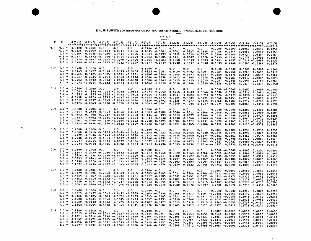
e e eSCALED ELEMENTS OF INFORMATION MATRIX FOR A MIXTURE OF TWO NORMAL DISTRIBUTIONS-

r = 1.0---_.

P D J (1,1) J (1,2) J (1,3) J (1,4) J (1, 5) J (2,2) J (2, 3) J (2.4) J (2.5) J (3.3) J (3,4) J (3.5) J (4.4) J (4,5) J (5,5)**•••••••** •••••••**•••••••****.** ••••••••••••••••••••••**••••••••••••••••••••••••••••••••••••••••••••••••••••••••••••••0.1 0.0 • 0.0100 0.0900 0.0 0.0 0.0 0.8100 0.0 0.0 0.0 0.0 0.0000 -0.0000 0.0050 0.0450 0.40500.2 • 0.0125 0.0859 -0.0441 -0.0041 -0.0306 o.8015 -0. 3501 0.0043 0.0327 0.1654 0.0066 0.0546 0.0068 0.0415 0.39590.4 • 0.0204 0.0718 -0.1089 -0.0101 -0.0505 0.7821 -0.6399 0.0119 0.0639 0.7137 0.0256 0.1869 0.0121 0.0291 0.37510.6 • 0.0317 0.0472 -0.1960 -0.0164 -0.0529 0.7642 -0.8205 0.0211 0.0887 1.7020 0.0439 0.3310 0.0179 0.0096 0.35550.8 • 0.0419 0.0177 -0.2807 -0.0200 -0.0406 o.7556 -0.8802 0.0258 0.1039 3.0509 0.0401 0.4397 0.0219 -0.0086 0.34301. a • 0.0488 -0.0092 -0.3357 -0.0212 -0.0208 0.7577 -0.8419 0.0230 0.1102 4.5698 0.0099 0.4964 0.0245 -0.0186 0.3376

0.2 0.0 • 0.0400 O. 1600 0.0 0.0 0.0 0.6400 0.0 0.0 0.0 0.0 0.0000 -0.0000 0.0200 0.0800 0.32000.2 • 0.0469 0.1477 -0.0838 -0.0133 -0.0468 0.6325 -0.3061 0.0139 0.0492 0.1601 0.0089 0.0356 0.0248 0.0698 0.31120.4 • 0.0645 0.1125 -0.1805 -0.0271 -0.0721 0.6186 -0.5389 0.0305 0.0871 0.6317 0.0259 0.1175 0.0351 0.0419 0.29440.6 • 0.0837 0.0635 -0.2753 -0.0368 -0.0710 0.6088 -0.6654 0.0423 0.1105 1.3516 0.0285 0.2057 0.0437 O. 008 8 0.28230.8 • 0.0982 0.0142 -0.3423 -0.0410 -0.0518 0.6080 -0.6943 0.0425 O. 1225 2.2015 0.0057 0.2760 0.0493 -0.0161 0.27671.0 • 0.1076 -0.0254 -0.3682 -0.0423 -0.0248 0.6168 -0.6518 0.031'1 0.1264 3.0629 -0.0338 0.3176 0.0534 -0.0271 0.2758

0.3 0.0 • 0.0900 0.2100 0.0 0.0 0.0 0.4900 0.0 0.0 0.0 0.0 0.0000 -0.0000 0.0450 0.1050 0.24500.2 • 0.1003 0.1896 -0.1209 -0.0248 -0.0531 0.4879 -0.2660 0.0255 0.0549 0.1566 0.0080 0.0210 0.0516 0.0883 0.24020.4 • 0.1232 0.1367 -0.2385 -0.0452 -0.0802 0.'1855 -0.4628 0.0481 0.0924 0.5873 0.0174 0.0723 0.0639 0.0488 0.23220.6 • 0.1454 0.0709 -0.3335 -0.0567 -0.0786 0.4862 -0.5672 0.0584 0.112'1 1.1924 0.0066 0.1343 0.0732 0.0077 0.22770.8 • 0.1612 0.0097 -0.3845 -0.0613 -0.0576 0.4920 -0.5902 0.0525 0.1217 1.8615 -0.0260 0.1907 0.079'1 -0.0205 0.22711. 0 • 0.1724 -0.0369 -0.3918 -0.0628 -0.0280 0.5041 -0.5543 0.0345 0.1246 2.5097 -0.0674 0.2300 0.0843 -0.0316 0.2290

0.4 0.0 • 0.1600 0.2400 0.0 0.0 0.0 0.3600 0.0 0.0 0.0 0.0 0.0000 -0.0000 0.0800 0.1200 0.18000.2 • 0.1711 0.2139 -0.1568 -0.0364 -0.0522 0.3641 -0.2284 0.0368 0.0532 0.1546 0.0046 0.0098 0.0865 0.0989 0.18010.4 • 0.1942 0.1498 -0.2917 -0.0622 -0.0800 0.3734 -0.3999 0.0629 0.0877 0.5644 0.0035 0.0398 0.0976 0.0524 0.18060.6 • 0.2153 0.0742 -0.3836 -0.0753 -0.0801 0.3833 -0.4948 0.0698 O. 1048 1.1169 -0.0188 0.0856 0.1061 0.0070 0.18240.8 • 0.2307 0.0066 -0.4238 -0.0804 -0.0603 0.3938 -0.5199 0.0582 O. 1121 1.7091 -0.0578 0.1347 0.1120 -0.0228 0.18491.0 • 0.2433 -0.0436 -0.4174 -0.0822 -0.0309 0.4072 -0.4927 0.0347 0.1145 2.2706 -0.0990 0.1742 0.1170 -0.0339 0.1885

f-'0.5 0.0 • 0.2500 0.2500 0.0 0.0 0.0 0.2500 0.0 0.0 0.0 0.0 0.0000 -0.0000 0.1250 0.1250 0.1250" 0.2 • 0.2588 0.2218 -0.1923 -0.0464 -0.0462 0.2588 -0.1923 0.0462 0.0464 0.1539 -0.0014 0.0014 0.1292 0.1023 0.1292

0.4 • 0.2772 0.1540 -0.3'143 -0.0769 -0.0738 o•277 2 -0.3443 0.0738 0.0769 0.5574 -0.0153 0.0153 0.1362 0.0535 0.13620.6 • 0.2940 0.0752 -0.'1359 -0.0917 -0.0771 0.2940 -0.4359 0.0771 0.0917 1.0942 -0.0488 0.0488 0.1423 0.0068 0.14230.8 • 0.3077 0.0055 -0.4671 -0.0977 -0.0606 0.3077 -0.4671 0.0606 0.0977 1.6643 -0.0927 0.0927 0.1469 -0.0235 0.14691.0 • 0.3211 -0.0459 -0.4496 -0.0998 -0.0333 0.3211 -0.4496 0.0333 0.0998 2.2016 -0.1330 0.1330 0.1516 -0.0346 0.1516

0.6 0.0 • 0.3600 0.2400 0.0 0.0 0.0 0.1600 0.0 0.0 0.0 0.0 0.0000 -0.0000 0.1800 0.1200 0.08000.2 • 0.3641 0.2139 -0.2284 -0.0532 -0.0368 0.1711 -0.1568 0.0522 0.0364 0.1546 -0.0098 -0.0046 0.1801 0.0989 0.08650.4 • 0.3734 0.1498 -0.3999 -0.0877 -0.0629 0.1942 -0.2917 0.0800 0.0622 0.5644 -0.0398 -0.0035 0.1806 0.0524 0.09760.6 • 0.3833 0.07'12 -0.4948 -0.1048 -0.0698 0.2153 -0.3836 0.0801 0.0753 1.1169 -0.0856 0.0188 0.1824 0.0070 0.10610.8 • 0.3938 0.0066 -0.5199 -0.1121 -0.0582 0.2307 -0.4238 0.0603 0.0804 1.7091 -0.1347 0.0578 0.1849 -0.0228 0.11201.0 • 0.4072 -0.0436 -0.4927 -0.1145 -0.0347 0.2433 -0.4174 0.0309 o•0822 2.2706 -0.1742 0.0990 0.1885 -0.0339 0.1170

0.7 0.0 • 0.4900 0.2100 0.0 0.0 0.0 0.0900 0.0 0.0 0.0 0.0 0.0000 -0.0000 0.2450 0.1050 0.04500.2 • 0.4879 0.1896 -0.2660 -0.0549 -0.0255 0.1003 -0.1209 0.0531 0.0248 0.1566 -0.0210 -0.0080 0.2402 0.0883 0.05160.4 • 0.4855 0.1367 -0.4628 -0.0924 -0.0481 0.1232 -0.2385 0.0802 0.0452 0.5873 -0.0723 -0.0174 0.2322 0.0488 0.06390.6 • 0.4862 0.0709 -0.5672 -0.1124 -0.0584 0.1454 -0.3335 0.0786 0.0567 1.1924 -0.1343 -0.0066 0.2277 0.0077 0.07320.8 • 0.4920 0.0097 -0.5902 -0.1217 -0.0525 0.1612 -0.3845 0.0576 0.0613 1.8615 -0.1907 0.0260 0.2271 -0.0205 0.07941.0 • 0.5041 -0.0369 -0.5543 -0.1246 -0.03'15 0.1724 -0.3918 0.0280 0.0628 2.5097 - 0.2300 0.0674 0.2290 -0.0316 0.0843

0.8 0.0 • 0.6400 0.1600 0.0 0.0 0.0 0.0400 0.0 0.0 0.0 0.0 0.0000 -0.0000 0.3200 0.0800 0.02000.2 • 0.6325 0.1477 -0.3061 -0.0492 -0.0139 0.0469 -0.0838 0.0468 0.0133 0.1601 -0.0356 -0.0089 0.3112 0.0698 0.02480.4 • 0.6186 0.1125 -0.5389 -0.0871 -0.0305 0.06115 -0.1805 0.0721 0.0271 0.6317 -0.1175 -0.0259 0.2944 0.0419 0.03510.6 • 0.6088 0.0635 -0.6654 -0.1105 -0.0423 0.0831 -0.2753 0.0710 0.0368 1.3516 -0.2057 -0.0285 0.2823 0.0088 0.04370.8 • 0.6080 0.0142 -0.6943 -0.1225 -0.01l25 0.0982 -0.3423 0.0518 0.0410 2.2015 -0.2760 -0.0057 0.2767 -0.0161 0.04931.0 • 0.6168 -0.0254 -0.6518 -0.1264 -0.0314 0.1076 -0.3682 0.0248 0.0423 3.0629 -0.3176 0.0338 0.2758 -0.0271 0.0534

0.9 0.0 • 0.8100 0.0900 0.0 0.0 0.0 0.0100 0.0 0.0 0.0 0.0 0.0000 -0.0000 0.4050 0.0450 0.00500.2 • 0.8015 0.0859 -0.3501 -0.0327 -0.0043 0.0125 -0.0441 0.0306 0.0041 0.1654 -0.0546 -0.0066 0.3959 0.0415 0.00680.4 • 0.7821 0.0718 -0.6399 -0.0639 -0.0119 0.0204 -0.1089 0.0505 0.0101 0.7137 -0.1869 -0.0256 0.3751 0.0291 0.01210.6 • 0.7642 0.0472 -0.8205 -0.0887 -0.0211 0.0317 -0.1960 0.0529 0.0164 1.7020 -0.3310 -0.0439 0.3555 0.0096 0.01790.8 • 0.7556 0.0177 -0.8802 -0.1039 -0.0258 0.0419 -0.2807 0.0406 0.0200 3.0509 -0.4397 -0.0401 0.3430 -0.0086 0.02191.0 • 0.7577 -0.0092 -0.8419 -0.1102 -0.0230 0.0488 -0.3357 0.0208 0.0212 4.5698 -0.4964 -0.0099 0.3376 -0.0186 0.0245

18

REFERENCES

[1] Behboodian, J., "On a mixture of normal distributions,"Biometrika 57 (1970), 215-216.

[2] , "Information for estimating the parameters in mixtures of ex-ponential and normal distributions," Ph.D. Thesis, Universityof Michigan, Ann Arbor, Michigan, (1964).

[3] Cohen, A.C., "Estimation in mixtures of two normal distributions,"Teohnometrios 9 (1967), 15-28.

[4] Day, N.E., "Estimating the components of a mixture of normal distri-butions," Biometrika 56 (1969), 463-474.

[5] Fisher, F..A., liThe truncated normal distribution," British Associationfor the Advanoement of Soienoe 3 Mathematioal Tab les 3 5,xxxiii-xxxiv.

[6] Hasselblad, V., "Estimation of parameters for a mixture of normal dis-tributions," Teohnometrios 8 (1966), 431-444.

[7] Hilderbrand, F.B., Introduotion to Numerioal Analysis3

McGraw-Hill Book Co., New York, 1956.

[8] Hill, B.M., "Information for estimating the proportions in mixtures ofexponential and normal distributions, II Jour. Amer. Stat. Assoo. 3

58 (1963), 918-932.

[9] Krylov, V.!., Approximate Caloulation of Integrals 3

Russian, 1959, translated, 1962, The Macmillan Co., New York.

[10] McCalla, toR., Introduotion to Numerioal Methods and FORTRAN

Programming, John Wiley & Sons, Inc., New York, 1967.