DISCUSSION PAPER SERIES

ABCD

www.cepr.org

Available online at: www.cepr.org/pubs/dps/DP6429.asp www.ssrn.com/xxx/xxx/xxx

No. 6429

FISCAL POLICY, LABOUR UNIONS AND MONETARY INSTITUTIONS:

THEIR LONG RUN IMPACT ON UNEMPLOYMENT, INFLATION

AND WELFARE

Alex Cukierman and Alberto Dalmazzo

INTERNATIONAL MACROECONOMICS, LABOUR ECONOMICS and PUBLIC

POLICY

ISSN 0265-8003

FISCAL POLICY, LABOUR UNIONS AND MONETARY INSTITUTIONS:

THEIR LONG RUN IMPACT ON UNEMPLOYMENT, INFLATION

AND WELFARE

Alex Cukierman, Tel Aviv University and CEPR Alberto Dalmazzo, University of Siena

Discussion Paper No. 6429

August 2007

Centre for Economic Policy Research 90–98 Goswell Rd, London EC1V 7RR, UK

Tel: (44 20) 7878 2900, Fax: (44 20) 7878 2999 Email: cepr@cepr.org, Website: www.cepr.org

This Discussion Paper is issued under the auspices of the Centre’s research programme in INTERNATIONAL MACROECONOMICS, LABOUR ECONOMICS and PUBLIC POLICY. Any opinions expressed here are those of the author(s) and not those of the Centre for Economic Policy Research. Research disseminated by CEPR may include views on policy, but the Centre itself takes no institutional policy positions.

The Centre for Economic Policy Research was established in 1983 as a private educational charity, to promote independent analysis and public discussion of open economies and the relations among them. It is pluralist and non-partisan, bringing economic research to bear on the analysis of medium- and long-run policy questions. Institutional (core) finance for the Centre has been provided through major grants from the Economic and Social Research Council, under which an ESRC Resource Centre operates within CEPR; the Esmée Fairbairn Charitable Trust; and the Bank of England. These organizations do not give prior review to the Centre’s publications, nor do they necessarily endorse the views expressed therein.

These Discussion Papers often represent preliminary or incomplete work, circulated to encourage discussion and comment. Citation and use of such a paper should take account of its provisional character.

Copyright: Alex Cukierman and Alberto Dalmazzo

CEPR Discussion Paper No. 6429

August 2007

ABSTRACT

Fiscal Policy, Labour Unions and Monetary Institutions: Their Long Run Impact on Unemployment, Inflation and Welfare*

Objectives and motivation: This paper considers the impact of interactions between fiscal policy and monetary institutions in the presence of unionized labour markets on economic outcomes and welfare in the long run. Two main classes of questions are investigated. First, what is the impact of exogenously given labour taxes and unemployment benefits on the choice of monetary policy by the central bank, on the choice of nominal wages by unions, on the choice of prices by monopolistically competitive firms and through them on unemployment, inflation and welfare? Second, how are labour taxes and redistribution chosen by a (Stackelberg leader) fiscal authority whose objectives are a weighted average of social welfare and of catering to the interests of political supporters, and how does the general equilibrium induced by this choice affect welfare? The framework of the paper is motivated by the European scene in which the fraction of the labour force covered by collective agreements dominates wage setting in the labour market.

"Players” and payoffs: The model economy features labour unions that maximize the expected real income of union members over states of employment and of unemployment, a central bank that strives to minimize the combined costs of inflation and of unemployment, and a continuum of monopolistically competitive firms, each of which maximizes its profits. The last part of the paper also features a fiscal authority that sets taxes and redistribution so as to maximize a combination of social welfare and of benefits to particular constituencies. Utility from consumption is characterized by means of a CES, Dixit-Stiglitz, utility function and (as in Sidrauski type models) money appears in the utility function.

Methodology and “players” strategies: The first question is investigated within a three stage game in which labour unions move first and commit to nominal wages and the central bank moves second and chooses the money supply. In the third and last stage each of a large number of monopolistically competitive firms picks its price. To deal with the second class of questions the game is expanded to feature a preliminary stage in which government chooses labour taxes and redistribution anticipating the subsequent responses of the other players. General equilibrium is characterized and used to find the impact of various economic and institutional parameters.

JEL Classification: E5, E6, H2, J3, J5 and L1 Keywords: fiscal monetary policy interactions, labour unions, monopolistic competition, monetary institutions, long run inflation unemployment tradeoff, welfare, politics and fiscal policy

Alex Cukierman Eitan Berglas School of Economics Tel-Aviv University Tel Aviv 69978 ISRAEL Email: alexcuk@post.tau.ac.il For further Discussion Papers by this author see: www.cepr.org/pubs/new-dps/dplist.asp?authorid=102723

Alberto Dalmazzo Dipartimento di Economia Politica Facoltà di Economia Piazza S. Francesco 7 I-53100 Siena ITALY Email: dalmazzo@unisi.it For further Discussion Papers by this author see: www.cepr.org/pubs/new-dps/dplist.asp?authorid=149123

*An earlier version of the paper was presented at the June 2007 Kiel Symposium on "The Phillips Curve and the Natural Rate of Unemployment". Submitted 07 August 2007

1 Introduction

This paper presents a general equilibrium microfounded macro framework characterized by im-

perfectly competitive goods and labor markets with sticky nominal wages and uses it to in-

vestigate the impact of economic structure and of fiscal and monetary policies on economic

performance in the long run. The framework of the paper is motivated by the European scene

in which the fraction of the labor force covered by collective agreements is large and in which

the degree of centralization of wage setting institutions varies across different countries.1

An important ingredient of our long run analysis, emphasized in some recent literature,

is that, in the presence of large wage setters, monetary policymaking institutions, like central

bank conservativeness (CBC) affect inflation as well as real variables even in the long run.2 As

a consequence the long run values of both unemployment and inflation are affected by the

level of CBC. The basic reason for this is that, when choosing its nominal (contractually set)

wage, a large wage setter internalizes the subsequent policy response of the monetary authority

to its own action. Since the nature of this response depends on CBC, nominal as well as real

wages, and the natural rate of unemployment depend on CBC. This mechanism does not appear

in most, now canonical, New-Keynesian macro models because those models are populated by

small price or wage setters that take monetary policy and other aggregate macroeconomic

variables as given.3 The paper does share with the New Keynesian literature the notion that

1In many European countries union membership is at least fifty percent. But, even in those countries in whichmembership is lower than fifty percent the fraction of the labor force actually covered by collective bargainingis substantially higher. This is achieved through various legal and other institutionalized extensions of unionwages to segments of the labor force that are not members of unions. According to OECD (1997) coverage ratesranged from 68% in Spain to 92% in France at the beginning of the nineties.

2A non exhaustive list includes Skott (1977), Cukierman and Lippi (1999), Soskice and Iversen (2000), Lippi(2003) and Coricelli, Cukierman and Dalmazzo (2006).

3For example the labor market in chapter 3 of Woodford (2003) is assumed to be competitive. AlthoughErceg, Henderson and Levin (2000) deviate from this paradigm by modeling labor suppliers as monopolisticallycompetitive agents, those agents do not believe that their individual actions affect the choice of monetary policyor other aggregate variables. One possible reason for these choices of modeling strategy is the fact that, in theUS, the fraction of the labor force covered by collective agreements is substantially smaller than in Europe. A

3

some nominal variables are sticky. But, unlike some early papers in this literature, it explores

the view that wages are substantially stickier than prices.4

Although, it is an important ingredient of our analysis the above mentioned mechanism is

only one of several mechanisms that serve as a starting point for the main issues that constitute

the focus of this paper. The paper discusses both positive and normative issues. The positive

questions concern the effects of economic structure and of policy instruments and institutions

on inflation, unemployment and the functional distribution of income in the long run. Economic

structure is characterized by the degree of competitiveness in the good’s markets and by the

degree of centralization of wage bargaining (CWB). Policy instruments and institutions are

characterized by labor taxes, unemployment benefits and CBC. The normative issues focus on

the impact of economic structure and policy instruments and institutions on economic welfare.

In comparison to the past, central banks in developed economies now enjoy high levels of

both legal and actual independence (or equivalently, effective conservativeness) and are expected

and encouraged to conduct policy mainly to achieve price stability. They possess, therefore,

high levels of effective CBC in Rogoff (1985) sense. It would appear, therefore, that monetary

policy is independent of politically motivated decisions in the fiscal area. The paper argues that

such a view is oversimplistic. Although direct political interferences with monetary policy are

rare, fiscal policy decisions regarding labor taxes and redistribution affect the monetary policy

decisions of even highly conservative central banks provided those banks are concerned, at least

to some extent, with real economic activity.5

Intuitively this occurs because fiscal parameters affect both inflation and unemployment,

recent attempt to introduce unions into a New-Keynesian framework appears in Gnocchi (2005).4For example King and Wolman (1999) assume that prices are sticky and that wages are fully flexible.

Friedman (1999) critisizes this assumption as being unrealistic. Our paper makes a step towards meeting thiscritisism while maintaining some analytical simplicity by exploring the diametrically opposite case in which wagesare contractually fixed and prices are flexible.

5That is provided they are flexible inflation targeters in Svensson (1997) sense.

4

and because the central bank (CB) cares about the values of those variables. The paper explores

the channels through which fiscal parameters like labor taxes and unemployment benefits affect

monetary policy decisions and through them economic performance. In addition, although

fiscal policymakers are taken as first movers with respect to the CB, the policy response they

expect from the bank affects their decisions. The first part of the paper abstracts from this

reverse causality by assuming that fiscal policy settings are exogenous. The latter part takes

it up by endogenizing fiscal policy. Together, those discussions provide a general equilibrium

analysis of the long run impact of fiscal and monetary policies on the economy while taking into

consideration the interactions between them.6

Following is a brief description of the analytical building blocks of the paper. The model

economy features a number of non atomistic labor unions each of which maximizes the expected

real income of a representative union member over states of employment and unemployment,

a central bank that strives to minimize the combined costs of inflation and of unemployment,

and a continuum of monopolistically competitive firms, each of which maximizes its individual

profits.

For given fiscal policy instruments the investigation is conducted within a three stage

game in which labor unions move first and commit to contractually fixed nominal wages and

the central bank moves second and chooses the money supply. In the third and last stage each

monopolistically competitive firm picks its price. The equilibrium outcomes are then used to

derive the implications for long run inflation, unemployment, income distribution and related

macroeconomic variables. This framework is also used to evaluate the impact of economic struc-

ture and policymaking institutions on welfare. To deal with the impact of monetary institutions

on the choice of fiscal instruments, the game is expanded to feature a preliminary stage in

which government chooses labor taxes and unemployment benefits, taking into consideration

6A first attempt to model the positive impact of those interactions in a somewhat different framework appearsin Cukierman and Dalmazzo (2006).

5

the subsequent responses of the other players to its own actions.

Methodologically, the paper provides a unified treatment of three distinct strands of re-

cent literature. One on strategic interactions between labor unions and the CB; another, mostly

empirical, on the effects of labor taxes on unemployment and competitiveness in the presence of

unionized labor markets; and a third on interactions between fiscal and monetary policies. Some

of the references in the first group have been mentionned above (see note 2). A recent exhaustive

empirical examination of the impact of fiscal and labor market institutions on unemployment in

the OECD countries appears in Nickell, Nunziata and Ochel (2005).7 Interactions between fiscal

and monetary policies under commitment and discretion within a single country are investigated

by Dixit and Lambertini (2003).8 An important difference between the last paper and ours is

that it posits (at least implicitly) a competitive labor market while our model features a small

number of unions making it possible to characterize the three ways strategic interaction among

fiscal policymakers, labor unions and the CB.9

Section 2 provides a general overview of the main building blocks of the model economy.

Section 3 characterizes general equilibrium of the economy for given fiscal policy instruments.

In particular it derives consumer’s demand functions, prices set by firms, the money supply cho-

sen by the CB, contractually fixed nominal wages set by labor unions and basic macroeconomic

variables like unemployment and inflation. Section 4 derives implications for real marginal costs,

the markup and the functional distribution of income, and section 5 summarizes general equi-

librium comparative statics results. Section 6 discusses the effects of economic structure, fiscal

7Related work includes Alesina and Perotti (1997), Daveri and Tabellini (2000) and Belot and van Ours(2001).

8Dixit (2001) and Dixit and Lambertini (2001) extend this analysis to the case of a monetary union.9Another difference is that they explore alternative combinations of regimes (discretion versus commitment)

for fiscal and monetary policies. By contrast, we consider a four stage game in which the fiscal authority movesfirst, labor unions move second, the central bank sets monetary policy in the third stage and individual pricesare set by monopolistically competitive firms in the last stage. The motivation for those timing assumptions isdiscussed in subsection 2.1 below

6

policy parameters and CBC on welfare. To this point all sections take fiscal policy instruments

as given. Section 7 endogenizes the choice of taxes and redistribution by adding a preliminary

stage to the previous three stages game. In this stage a government that cares about both redis-

tribution and social welfare chooses taxes, taking into consideration the subsequent responses

of unions, the CB and price setters. This is followed by concluding remarks.

2 An overview of the model

There is a continuum of monopolistically competitive firms, whose mass is one, and n equally

sized labor unions that organize the entire labor force. Each firm is owned by an entrepeneur

whose income consists of the firm’s profits. The mass of firms in the economy is one. Each

monopolistic union covers the labor force of a fraction 1/n of the firms. A quantity L0 of

workers is attached to each firm. Without loss of generality, all firms whose labor force is

represented by union i are assigned to the contiguous subinterval ( in, i+1

n) of the unit interval,

where i = 0, 1..., n− 1.10 Utility of an individual in the economy is given by:

U =

µC

γ

¶γ µM/P

1− γ

¶1−γ+ (1− λ)R, γ ∈ (0, 1) (1)

Here C is a Dixit-Stiglitz (1977) consumption aggregator

C =

µZ 1

0

Cθ−1θ

j dj

¶ θθ−1

, θ > 1 (2)

of imperfectly substituable consumption varieties, Cj , whose mass is equal to one and θ is the

(constant across varieties) elasticity of substitution between any pair of varieties. M denotes

the nominal money stock held by the individual, and the price level P (equal conceptually to

10This part of the the model builds on Coricelli, Cukierman and Dalmazzo (2006).

7

the minimum cost of providing the utility level C) is given by:

P =

µZ 1

0

P 1−θj

¶ 11−θ

(3)

where Pj is the price of variety j. A worker can be either employed or unemployed. R denotes

the difference between his utility from leisure when unemployed and employed so that λ = 0

when he is unemployed and λ = 1 when he is employed. Since all firm owners (entrepeneurs)

must forego leisure to manage their firms λ = 1 for each entrepeneur.11 Each individual, whether

a worker or a capitalist, possesses an initial endowment of money, M. This endowment is the

same for all individuals.

Let Acs denote total nominal resources available to individual s in class c where c =

EW,UW,E. Here EW,UW,E stand for "employed worker", "unemployed worker", and "em-

ployer" respectively. The budget constraint of individual s states that the nominal resources at

his disposition are used to satisfy his consumption demands for the different varieties, Ccsj, plus

his demand for nominal money balances, Mcs. It is given by

Acs =Mcs +

Z 1

0

PjCcsjdj, s = EW,UW,E (4)

where

AEWs =WEWs +M + TRW , AUWs = B +M + TRW , As = Πs +M + TRE. (5)

Here WEWs is the net nominal wage earned by employed worker s, B ≥ 0 is an unemployment

benefit paid by government to each unemployed worker, Πs is the profit received by firm owner

s, and TRW ,and TRE are governmental transfers to each worker and employer respectively.

11This part of the model utilizes some of the structure from Blanchard and Kiyotaki (1987) and chapter 8 ofBlanchard and Fischer (1988).

8

For simplicity the transfers to each worker and employers are assumed to be the same across

workers and employers respectively. Each individual, s, whether worker or entrepeneur, chooses

consumption varieties, Ccsj, j ∈ [0, 1] and nominal money balances, Mcs, so as to maximize

utility, (1), subject to the budget constraint (4). In the rest of the paper we drop the individual

index, s, whenever there is no risk of confusion.

Government raises taxes on labor and utilizes the proceeds to finance unemployment

benefits, as well as other transfers. As in Alesina and Perotti (1997), there are two types of

taxes. A social security tax paid by the employer (at rate σ), and an income tax (at rate υ).

Denoting by Wg the gross wage paid to an employee, a firm bears a per-worker cost of labor

equal to (1 + σ)Wg, while the worker receives a net wage equal to W = (1− ν)Wg.12 Thus, the

ratio between the net wage and the cost of labor to the firm is given by 1−ν1+σ≡ (1− t), and the

cost of labor to the firm can be written as W(1−t) . Taking (natural) logarithms the last equation,

can be reformulated as logW − log(1− t) ≡ w + τ , where − log(1− t) ≡ τ > 0.

Given taxation, the real profits of firm j, whose workforce belongs to union i are given

by

Πij

P=

Pj

PCaj −

Wi

P (1− t)Lij, j ∈ [0, 1] (6)

where Caj denotes the aggregate demand for variety j. Taking the nominal wage, Wi, and the

general price level, P , as given each firm chooses the price, Pj, of the variety it sells so as to

maximize profits subject to the production function

Yj = Lαij, α < 1. (7)

Yj is the amount of this variety that is produced and Lij is the number of workers employed by

12Since the discussion here is a generic one we omit the indices of the particular worker and firm.

9

firm j.

Monetary institutions are represented by a central bank (CB) that dislikes both inflation,

π, and unemployment, u. As in Coricelli, Cukierman and Dalmazzo (2006), the CB chooses the

money supply so to minimize the combined costs of inflation and of unemployment that are

given by

Γ = u2 + I · π2, I ∈ [0,∞). (8)

As in Rogoff (1985), the parameter I measures the relative importance that the CB assigns to

the objective of low inflation versus low unemployment. This parameter is also known as the

degree of CB conservativeness (CBC).

The probability that a member of union i will be unemployed is identical and independent

across the union’s members so that the probability that any union member is unemployed is

equal to the rate of unemployment among its members. Taking the nominal wages of other

unions as given, each union, i, sets the nominal wage, Wi, for its members so as to maximize

the expected utility of a representative member. This expected utility is given by

vi = (1− ui)VEW (AEW ) + uiVUW (AUW ) (9)

where ui is the unemployment rate among union i’s members and, VEW (.) and VUW (.) are

the individually maximal values of utility of employed and unemployed workers expressed as

functions of the resources available to each type of worker.

We assume that the "replacement ratio" BWiis constant and equal to β < 1 so that

BP= βWi

P. We also postulate that the level of maximized utility when employed is larger than

the level of maximized utility when unemployed at all real wages above than or equal to the

competitive one so that

VEW (AEW ) ≥ VUW (AUW ). (10)

10

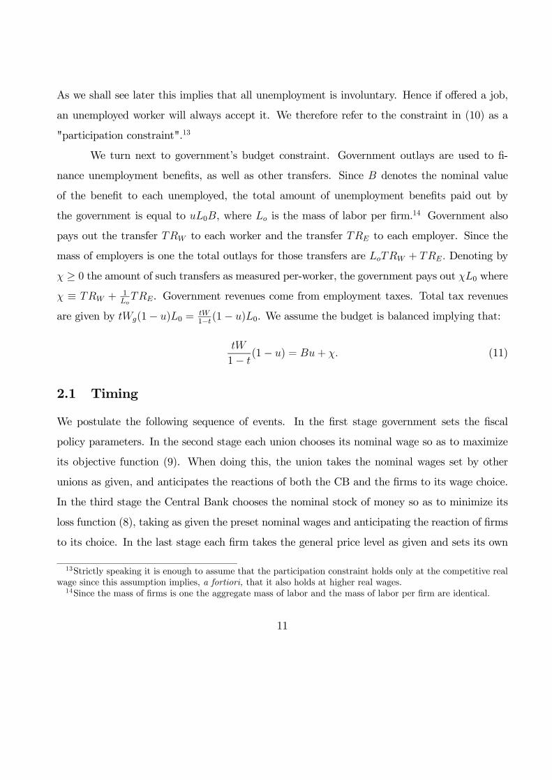
As we shall see later this implies that all unemployment is involuntary. Hence if offered a job,

an unemployed worker will always accept it. We therefore refer to the constraint in (10) as a

"participation constraint".13

We turn next to government’s budget constraint. Government outlays are used to fi-

nance unemployment benefits, as well as other transfers. Since B denotes the nominal value

of the benefit to each unemployed, the total amount of unemployment benefits paid out by

the government is equal to uL0B, where Lo is the mass of labor per firm.14 Government also

pays out the transfer TRW to each worker and the transfer TRE to each employer. Since the

mass of employers is one the total outlays for those transfers are LoTRW + TRE. Denoting by

χ ≥ 0 the amount of such transfers as measured per-worker, the government pays out χL0 where

χ ≡ TRW + 1LoTRE. Government revenues come from employment taxes. Total tax revenues

are given by tWg(1− u)L0 =tW1−t(1− u)L0. We assume the budget is balanced implying that:

tW

1− t(1− u) = Bu+ χ. (11)

2.1 Timing

We postulate the following sequence of events. In the first stage government sets the fiscal

policy parameters. In the second stage each union chooses its nominal wage so as to maximize

its objective function (9). When doing this, the union takes the nominal wages set by other

unions as given, and anticipates the reactions of both the CB and the firms to its wage choice.

In the third stage the Central Bank chooses the nominal stock of money so as to minimize its

loss function (8), taking as given the preset nominal wages and anticipating the reaction of firms

to its choice. In the last stage each firm takes the general price level as given and sets its own

13Strictly speaking it is enough to assume that the participation constraint holds only at the competitive realwage since this assumption implies, a fortiori, that it also holds at higher real wages.14Since the mass of firms is one the aggregate mass of labor and the mass of labor per firm are identical.

11

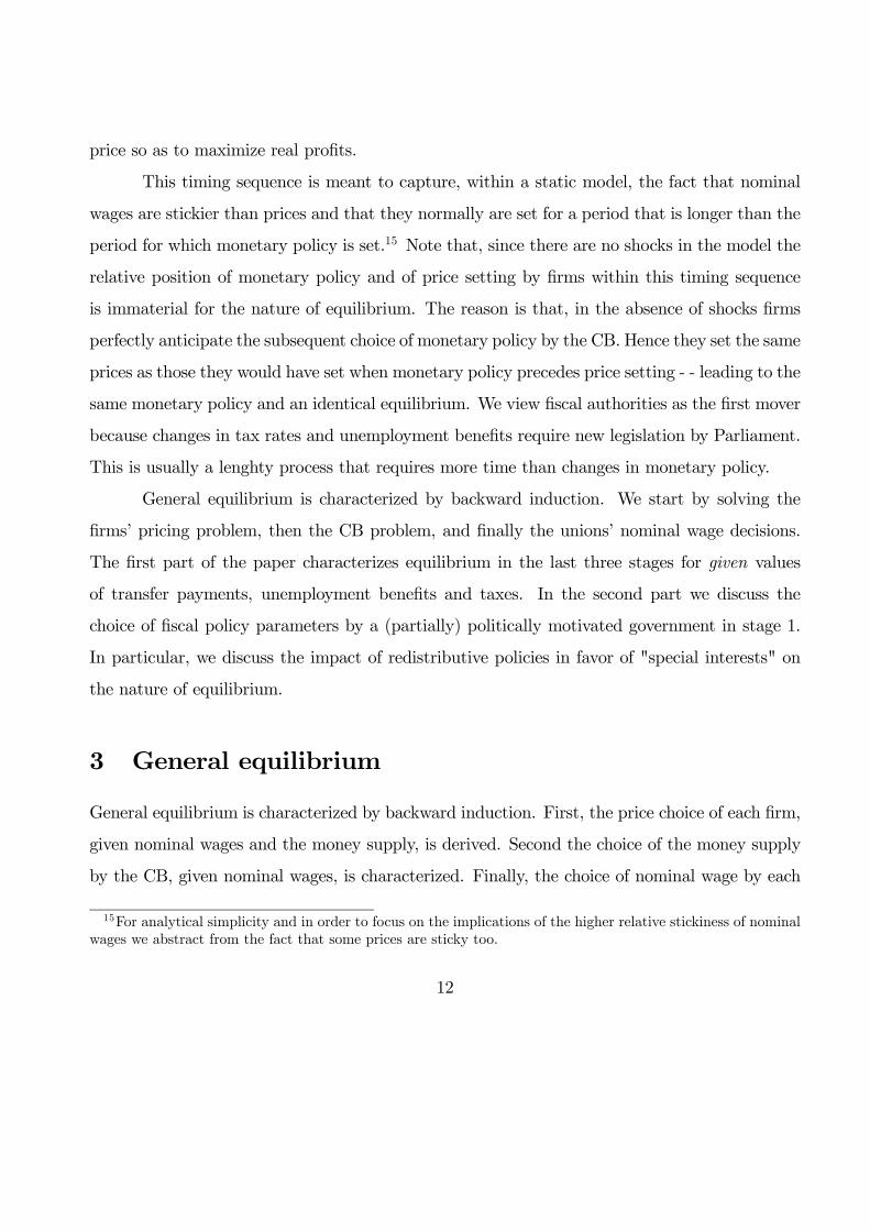
price so as to maximize real profits.

This timing sequence is meant to capture, within a static model, the fact that nominal

wages are stickier than prices and that they normally are set for a period that is longer than the

period for which monetary policy is set.15 Note that, since there are no shocks in the model the

relative position of monetary policy and of price setting by firms within this timing sequence

is immaterial for the nature of equilibrium. The reason is that, in the absence of shocks firms

perfectly anticipate the subsequent choice of monetary policy by the CB. Hence they set the same

prices as those they would have set when monetary policy precedes price setting - - leading to the

same monetary policy and an identical equilibrium. We view fiscal authorities as the first mover

because changes in tax rates and unemployment benefits require new legislation by Parliament.

This is usually a lenghty process that requires more time than changes in monetary policy.

General equilibrium is characterized by backward induction. We start by solving the

firms’ pricing problem, then the CB problem, and finally the unions’ nominal wage decisions.

The first part of the paper characterizes equilibrium in the last three stages for given values

of transfer payments, unemployment benefits and taxes. In the second part we discuss the

choice of fiscal policy parameters by a (partially) politically motivated government in stage 1.

In particular, we discuss the impact of redistributive policies in favor of "special interests" on

the nature of equilibrium.

3 General equilibrium

General equilibrium is characterized by backward induction. First, the price choice of each firm,

given nominal wages and the money supply, is derived. Second the choice of the money supply

by the CB, given nominal wages, is characterized. Finally, the choice of nominal wage by each

15For analytical simplicity and in order to focus on the implications of the higher relative stickiness of nominalwages we abstract from the fact that some prices are sticky too.

12

union is calculated. Characterization of price setting decisions by each firm requires knowledge

of the demand facing each firm. Since this demand depends on the behavior of consumers we

start with the maximization problem of a typical consumer.

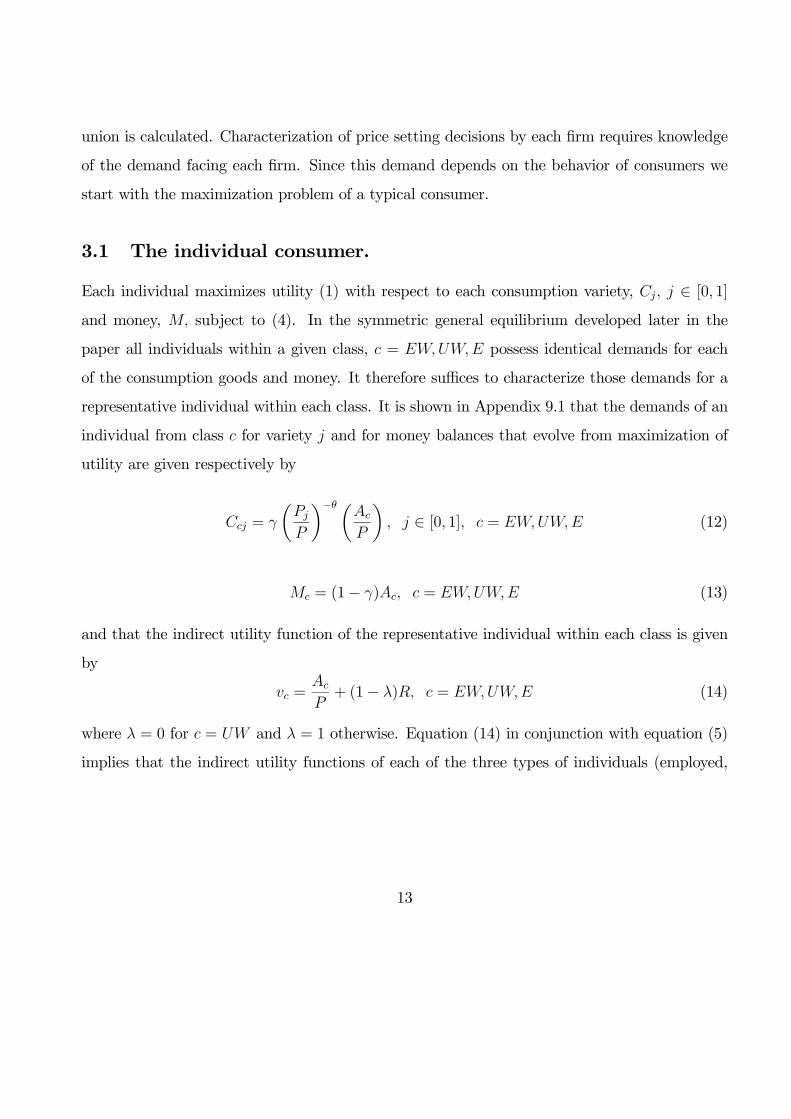
3.1 The individual consumer.

Each individual maximizes utility (1) with respect to each consumption variety, Cj, j ∈ [0, 1]

and money, M, subject to (4). In the symmetric general equilibrium developed later in the

paper all individuals within a given class, c = EW,UW,E possess identical demands for each

of the consumption goods and money. It therefore suffices to characterize those demands for a

representative individual within each class. It is shown in Appendix 9.1 that the demands of an

individual from class c for variety j and for money balances that evolve from maximization of

utility are given respectively by

Ccj = γ

µPj

P

¶−θ µAc

P

¶, j ∈ [0, 1], c = EW,UW,E (12)

Mc = (1− γ)Ac, c = EW,UW,E (13)

and that the indirect utility function of the representative individual within each class is given

by

vc =Ac

P+ (1− λ)R, c = EW,UW,E (14)

where λ = 0 for c = UW and λ = 1 otherwise. Equation (14) in conjunction with equation (5)

implies that the indirect utility functions of each of the three types of individuals (employed,

13

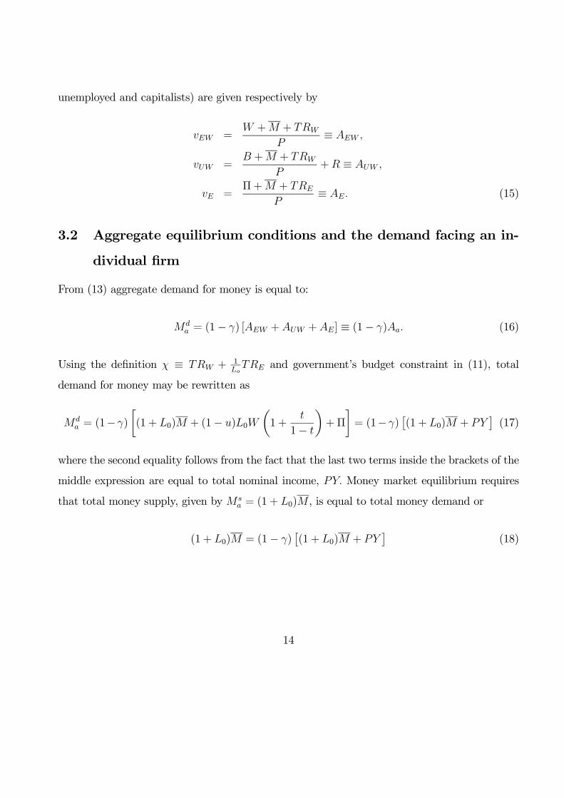
unemployed and capitalists) are given respectively by

vEW =W +M + TRW

P≡ AEW ,

vUW =B +M + TRW

P+R ≡ AUW ,

vE =Π+M + TRE

P≡ AE. (15)

3.2 Aggregate equilibrium conditions and the demand facing an in-

dividual firm

From (13) aggregate demand for money is equal to:

Mda = (1− γ) [AEW +AUW +AE] ≡ (1− γ)Aa. (16)

Using the definition χ ≡ TRW + 1LoTRE and government’s budget constraint in (11), total

demand for money may be rewritten as

Mda = (1−γ)

∙(1 + L0)M + (1− u)L0W

µ1 +

t

1− t

¶+Π

¸= (1−γ)

£(1 + L0)M + PY

¤(17)

where the second equality follows from the fact that the last two terms inside the brackets of the

middle expression are equal to total nominal income, PY. Money market equilibrium requires

that total money supply, given by M sa = (1 + L0)M , is equal to total money demand or

(1 + L0)M = (1− γ)£(1 + L0)M + PY

¤(18)

14

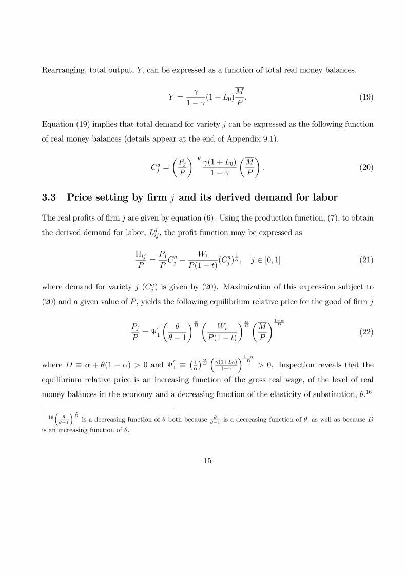
Rearranging, total output, Y, can be expressed as a function of total real money balances.

Y =γ

1− γ(1 + L0)

M

P. (19)

Equation (19) implies that total demand for variety j can be expressed as the following function

of real money balances (details appear at the end of Appendix 9.1).

Caj =

µPj

P

¶−θγ(1 + L0)

1− γ

µM

P

¶. (20)

3.3 Price setting by firm j and its derived demand for labor

The real profits of firm j are given by equation (6). Using the production function, (7), to obtain

the derived demand for labor, Ldij, the profit function may be expressed as

Πij

P=

Pj

PCaj −

Wi

P (1− t)(Ca

j )1α , j ∈ [0, 1] (21)

where demand for variety j (Caj ) is given by (20). Maximization of this expression subject to

(20) and a given value of P , yields the following equilibrium relative price for the good of firm j

Pj

P= Ψ

01

µθ

θ − 1

¶ αDµ

Wi

P (1− t)

¶ αDµM

P

¶1−αD

(22)

where D ≡ α + θ(1 − α) > 0 and Ψ01 ≡

¡1α

¢ αD

³γ(1+L0)1−γ

´ 1−αD

> 0. Inspection reveals that the

equilibrium relative price is an increasing function of the gross real wage, of the level of real

money balances in the economy and a decreasing function of the elasticity of substitution, θ.16

16³

θθ−1

´ αD

is a decreasing function of θ both because θθ−1 is a decreasing function of θ, as well as because D

is an increasing function of θ.

15

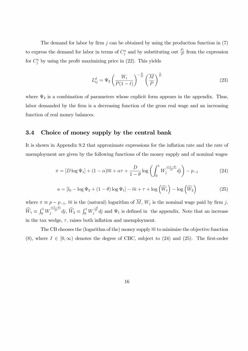
The demand for labor by firm j can be obtained by using the production function in (7)

to express the demand for labor in terms of Caj and by substituting out

PjPfrom the expression

for Caj by using the profit maximizing price in (22). This yields

Ldij = Ψ2

µWi

P (1− t)

¶− θDµM

P

¶ 1D

(23)

where Ψ2 is a combination of parameters whose explicit form appears in the appendix. Thus,

labor demanded by the firm is a decreasing function of the gross real wage and an increasing

function of real money balances.

3.4 Choice of money supply by the central bank

It is shown in Appendix 9.2 that approximate expressions for the inflation rate and the rate of

unemployment are given by the following functions of the money supply and of nominal wages

π = [D logΨ1] + (1− α)m+ ατ +D

1− θlog

µZ 1

0

Wα(1−θ)

Dj dj

¶− p−1 (24)

u = [l0 − logΨ2 + (1− θ) logΨ1]−m+ τ + log³cW1

´− log

³cW2

´(25)

where π ≡ p− p−1, m is the (natural) logarithm of M , Wj is the nominal wage paid by firm j,cW1 ≡R 10W

α(1−θ)D

j dj, cW2 ≡R 10W

−θDj dj and Ψ1 is defined in the appendix. Note that an increase

in the tax wedge, τ , raises both inflation and unemployment.

The CB chooses the (logarithm of the) money supplym to minimize the objective function

(8), where I ∈ [0,∞) denotes the degree of CBC, subject to (24) and (25). The first-order

16

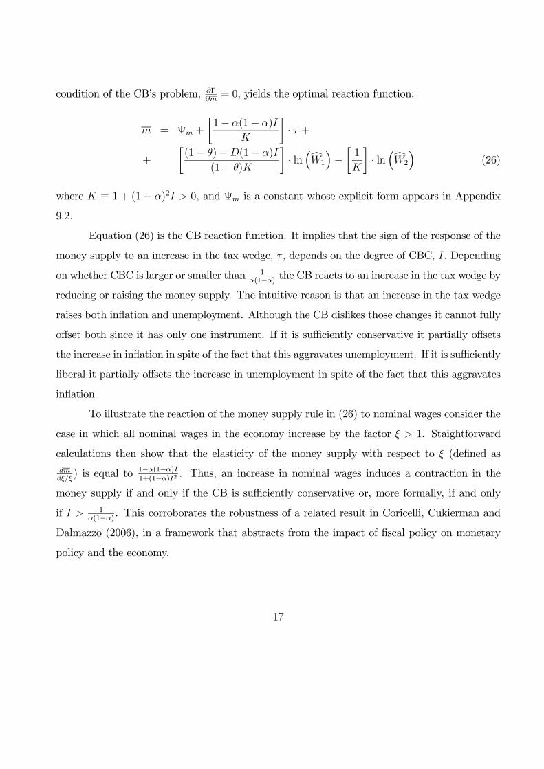
condition of the CB’s problem, ∂Γ∂m= 0, yields the optimal reaction function:

m = Ψm +

∙1− α(1− α)I

K

¸· τ +

+

∙(1− θ)−D(1− α)I

(1− θ)K

¸· ln³cW1

´−∙1

K

¸· ln³cW2

´(26)

where K ≡ 1 + (1− α)2I > 0, and Ψm is a constant whose explicit form appears in Appendix

9.2.

Equation (26) is the CB reaction function. It implies that the sign of the response of the

money supply to an increase in the tax wedge, τ , depends on the degree of CBC, I. Depending

on whether CBC is larger or smaller than 1α(1−α) the CB reacts to an increase in the tax wedge by

reducing or raising the money supply. The intuitive reason is that an increase in the tax wedge

raises both inflation and unemployment. Although the CB dislikes those changes it cannot fully

offset both since it has only one instrument. If it is sufficiently conservative it partially offsets

the increase in inflation in spite of the fact that this aggravates unemployment. If it is sufficiently

liberal it partially offsets the increase in unemployment in spite of the fact that this aggravates

inflation.

To illustrate the reaction of the money supply rule in (26) to nominal wages consider the

case in which all nominal wages in the economy increase by the factor ξ > 1. Staightforward

calculations then show that the elasticity of the money supply with respect to ξ (defined asdmdξ/ξ) is equal to 1−α(1−α)I

1+(1−α)I2 . Thus, an increase in nominal wages induces a contraction in the

money supply if and only if the CB is sufficiently conservative or, more formally, if and only

if I > 1α(1−α) . This corroborates the robustness of a related result in Coricelli, Cukierman and

Dalmazzo (2006), in a framework that abstracts from the impact of fiscal policy on monetary

policy and the economy.

17

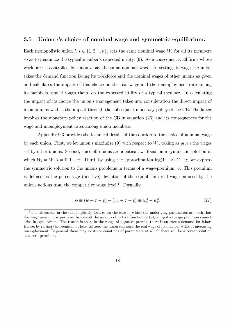
3.5 Union i’s choice of nominal wage and symmetric equilibrium.

Each monopolistic union i, i ∈ {1, 2, .., n}, sets the same nominal wage Wi for all its members

so as to maximize the typical member’s expected utility, (9). As a consequence, all firms whose

workforce is controlled by union i pay the same nominal wage. In setting its wage the union

takes the demand function facing its workforce and the nominal wages of other unions as given

and calculates the impact of this choice on the real wage and the unemployment rate among

its members, and through them, on the expected utility of a typical member. In calculating

the impact of its choice the union’s management takes into consideration the direct impact of

its action, as well as the impact through the subsequent monetary policy of the CB. The latter

involves the monetary policy reaction of the CB in equation (26) and its consequences for the

wage and unemployment rates among union members.

Appendix 9.3 provides the technical details of the solution to the choice of nominal wage

by each union. First, we let union i maximize (9) with respect to Wi, taking as given the wages

set by other unions. Second, since all unions are identical, we focus on a symmetric solution in

which Wi = W , i = 0, 1..., n. Third, by using the approximation log(1 − x) ∼= −x, we express

the symmetric solution to the unions problems in terms of a wage-premium, φ. This premium

is defined as the percentage (positive) deviation of the equilibrium real wage induced by the

unions actions from the competitive wage level.17 Formally

φ ≡ (w + τ − p)− (wc + τ − p) ≡ wgr − wg

rc (27)

17The discussion in the text implicitly focuses on the case in which the underlying parameters are such thatthe wage premium is positive. In view of the union’s objective function in (9), a negative wage premium cannotarise in equilibrium. The reason is that, in the range of negative premia, there is an excess demand for labor.Hence, by raising the premium at least till zero the union can raise the real wage of its member without increasingunemployment. In general there may exist combinations of parameters at which there will be a corner solutionat a zero premium.

18

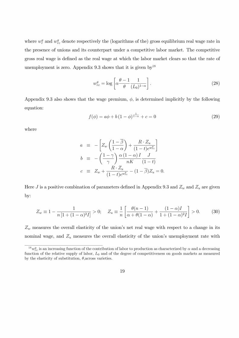
where wgr and w

grc denote respectively the (logarithms of the) gross equilibrium real wage rate in

the presence of unions and its counterpart under a competitive labor market. The competitive

gross real wage is defined as the real wage at which the labor market clears so that the rate of

unemployment is zero. Appendix 9.3 shows that it is given by18

wgrc = log

∙αθ − 1θ

1

(L0)1−α

¸. (28)

Appendix 9.3 also shows that the wage premium, φ, is determined implicitly by the following

equation:

f(φ) = aφ+ b (1− φ)1

1−α + c = 0 (29)

where

a ≡ −∙Zw

µ1− β

1− α

¶+

R · Zu

(1− t)ewgrc

¸b ≡ −

µ1− γ

γ

¶α (1− α) I

nK

J

(1− t)

c ≡ Zw +R · Zu

(1− t)ewgrc− (1− β)Zu = 0.

Here J is a positive combination of parameters defined in Appendix 9.3 and Zw and Zu are given

by:

Zw ≡ 1−1

n [1 + (1− α)2I]> 0; Zu ≡

1

n

∙θ(n− 1)

α+ θ(1− α)+

(1− α)I

1 + (1− α)2I

¸> 0. (30)

Zw measures the overall elasticity of the union’s net real wage with respect to a change in its

nominal wage, and Zu measures the overall elasticity of the union’s unemployment rate with

18wgrc is an increasing function of the contribution of labor to production as characterized by α and a decreasing

function of the relative supply of labor, L0 and of the degree of competitiveness on goods markets as measuredby the elasticity of substitution, θ,across varieties.

19

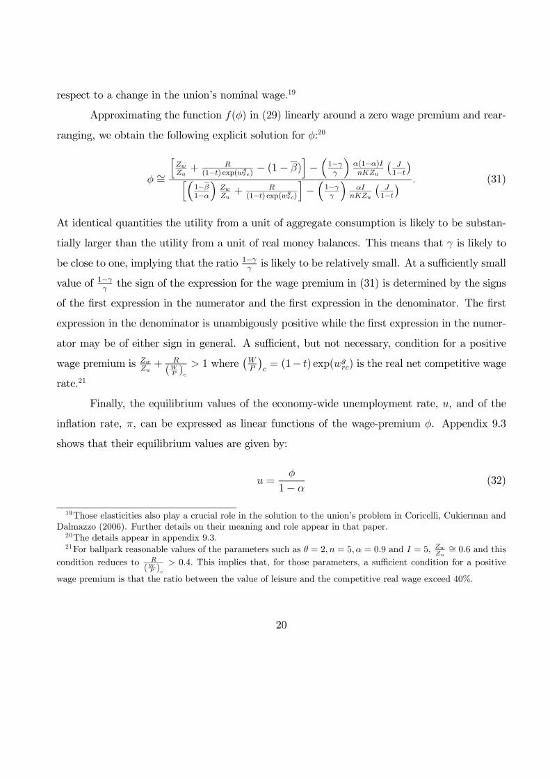
respect to a change in the union’s nominal wage.19

Approximating the function f(φ) in (29) linearly around a zero wage premium and rear-

ranging, we obtain the following explicit solution for φ:20

φ ∼=

hZwZu+ R

(1−t) exp(wgrc) − (1− β)i−³1−γγ

´α(1−α)InKZu

¡J1−t¢h³

1−β1−α

´ZwZu+ R

(1−t) exp(wgrc)

i−³1−γγ

´αI

nKZu

¡J1−t¢ . (31)

At identical quantities the utility from a unit of aggregate consumption is likely to be substan-

tially larger than the utility from a unit of real money balances. This means that γ is likely to

be close to one, implying that the ratio 1−γγis likely to be relatively small. At a sufficiently small

value of 1−γγthe sign of the expression for the wage premium in (31) is determined by the signs

of the first expression in the numerator and the first expression in the denominator. The first

expression in the denominator is unambigously positive while the first expression in the numer-

ator may be of either sign in general. A sufficient, but not necessary, condition for a positive

wage premium is ZwZu+ R

(WP )c> 1 where

¡WP

¢c= (1− t) exp(wg

rc) is the real net competitive wage

rate.21

Finally, the equilibrium values of the economy-wide unemployment rate, u, and of the

inflation rate, π, can be expressed as linear functions of the wage-premium φ. Appendix 9.3

shows that their equilibrium values are given by:

u =φ

1− α(32)

19Those elasticities also play a crucial role in the solution to the union’s problem in Coricelli, Cukierman andDalmazzo (2006). Further details on their meaning and role appear in that paper.20The details appear in appendix 9.3.21For ballpark reasonable values of the parameters such as θ = 2, n = 5, α = 0.9 and I = 5, Zw

Zu∼= 0.6 and this

condition reduces to R

(WP )c> 0.4. This implies that, for those parameters, a sufficient condition for a positive

wage premium is that the ratio between the value of leisure and the competitive real wage exceed 40%.

20

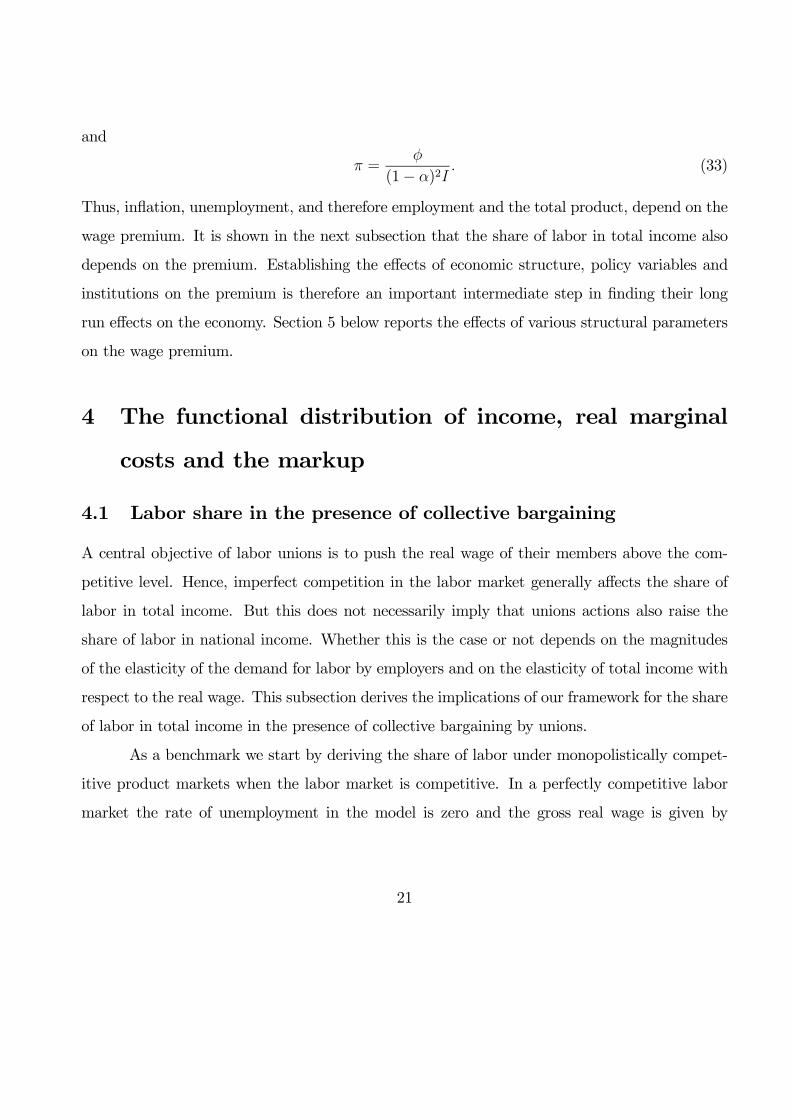
and

π =φ

(1− α)2I. (33)

Thus, inflation, unemployment, and therefore employment and the total product, depend on the

wage premium. It is shown in the next subsection that the share of labor in total income also

depends on the premium. Establishing the effects of economic structure, policy variables and

institutions on the premium is therefore an important intermediate step in finding their long

run effects on the economy. Section 5 below reports the effects of various structural parameters

on the wage premium.

4 The functional distribution of income, real marginal

costs and the markup

4.1 Labor share in the presence of collective bargaining

A central objective of labor unions is to push the real wage of their members above the com-

petitive level. Hence, imperfect competition in the labor market generally affects the share of

labor in total income. But this does not necessarily imply that unions actions also raise the

share of labor in national income. Whether this is the case or not depends on the magnitudes

of the elasticity of the demand for labor by employers and on the elasticity of total income with

respect to the real wage. This subsection derives the implications of our framework for the share

of labor in total income in the presence of collective bargaining by unions.

As a benchmark we start by deriving the share of labor under monopolistically compet-

itive product markets when the labor market is competitive. In a perfectly competitive labor

market the rate of unemployment in the model is zero and the gross real wage is given by

21

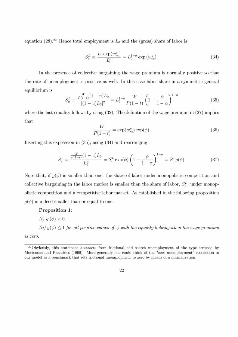
equation (28).22 Hence total employment is L0 and the (gross) share of labor is

SLc ≡

L0 exp(wgrc)

Lα0

= L1−α0 exp (wgrc) . (34)

In the presence of collective bargaining the wage premium is normally positive so that

the rate of unemployment is positive as well. In this case labor share in a symmetric general

equilibrium is

SLu ≡

WP (1−t)(1− u)L0

[(1− u)L0]α = L1−α0

W

P (1− t)

µ1− φ

1− α

¶1−α(35)

where the last equality follows by using (32). The definition of the wage premium in (27).implies

thatW

P (1− t)= exp(wg

rc) exp(φ). (36)

Inserting this expression in (35), using (34) and rearranging

SLu ≡

WP (1−t)(1− u)L0

Lα0

= SLc exp(φ)

µ1− φ

1− α

¶1−α≡ SL

c g(φ). (37)

Note that, if g(φ) is smaller than one, the share of labor under monopolistic competition and

collective bargaining in the labor market is smaller than the share of labor, SLc , under monop-

olistic competition and a competitive labor market. As established in the following proposition

g(φ) is indeed smaller than or equal to one.

Proposition 1:

(i) g0(φ) < 0.

(ii) g(φ) ≤ 1 for all positive values of φ with the equality holding when the wage premium

is zero.

22Obviously, this statement abstracts from frictional and search unemployment of the type stressed byMortensen and Pissarides (1999). More generally one could think of the "zero unemployment" restriction inour model as a benchmark that sets frictional unemployment to zero by means of a normalization.

22

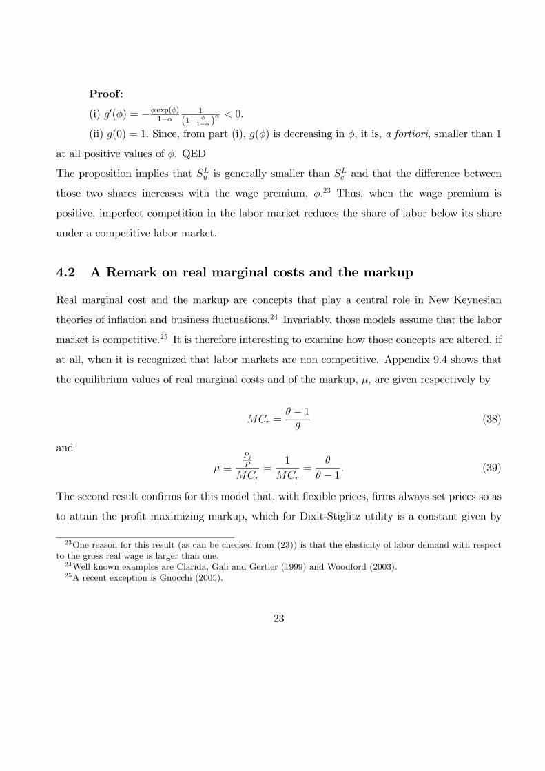
Proof :

(i) g0(φ) = −φ exp(φ)1−α

1

(1− φ1−α)

α < 0.

(ii) g(0) = 1. Since, from part (i), g(φ) is decreasing in φ, it is, a fortiori, smaller than 1

at all positive values of φ. QED

The proposition implies that SLu is generally smaller than SL

c and that the difference between

those two shares increases with the wage premium, φ.23 Thus, when the wage premium is

positive, imperfect competition in the labor market reduces the share of labor below its share

under a competitive labor market.

4.2 A Remark on real marginal costs and the markup

Real marginal cost and the markup are concepts that play a central role in New Keynesian

theories of inflation and business fluctuations.24 Invariably, those models assume that the labor

market is competitive.25 It is therefore interesting to examine how those concepts are altered, if

at all, when it is recognized that labor markets are non competitive. Appendix 9.4 shows that

the equilibrium values of real marginal costs and of the markup, µ, are given respectively by

MCr =θ − 1θ

(38)

and

µ ≡PjP

MCr=

1

MCr=

θ

θ − 1 . (39)

The second result confirms for this model that, with flexible prices, firms always set prices so as

to attain the profit maximizing markup, which for Dixit-Stiglitz utility is a constant given by

23One reason for this result (as can be checked from (23)) is that the elasticity of labor demand with respectto the gross real wage is larger than one.24Well known examples are Clarida, Gali and Gertler (1999) and Woodford (2003).25A recent exception is Gnocchi (2005).

23

equation (39).

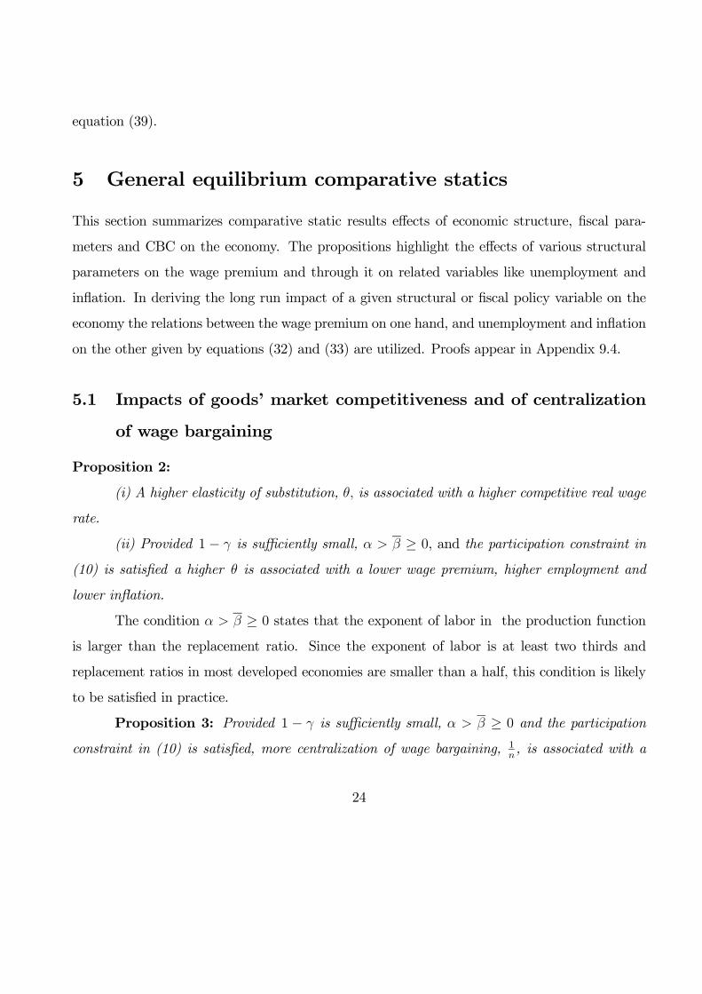
5 General equilibrium comparative statics

This section summarizes comparative static results effects of economic structure, fiscal para-

meters and CBC on the economy. The propositions highlight the effects of various structural

parameters on the wage premium and through it on related variables like unemployment and

inflation. In deriving the long run impact of a given structural or fiscal policy variable on the

economy the relations between the wage premium on one hand, and unemployment and inflation

on the other given by equations (32) and (33) are utilized. Proofs appear in Appendix 9.4.

5.1 Impacts of goods’ market competitiveness and of centralization

of wage bargaining

Proposition 2:

(i) A higher elasticity of substitution, θ, is associated with a higher competitive real wage

rate.

(ii) Provided 1 − γ is sufficiently small, α > β ≥ 0, and the participation constraint in

(10) is satisfied a higher θ is associated with a lower wage premium, higher employment and

lower inflation.

The condition α > β ≥ 0 states that the exponent of labor in the production function

is larger than the replacement ratio. Since the exponent of labor is at least two thirds and

replacement ratios in most developed economies are smaller than a half, this condition is likely

to be satisfied in practice.

Proposition 3: Provided 1 − γ is sufficiently small, α > β ≥ 0 and the participation

constraint in (10) is satisfied, more centralization of wage bargaining, 1n, is associated with a

24

lower wage premium, higher employment and lower inflation.

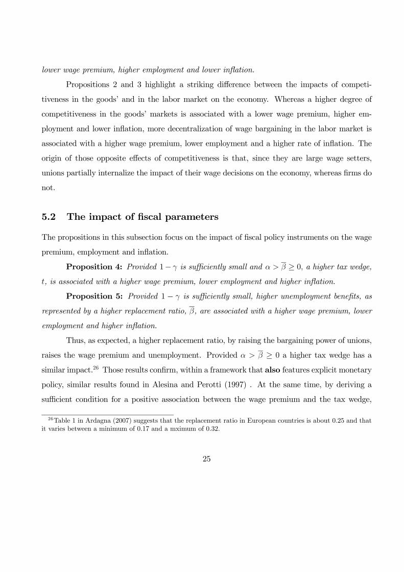
Propositions 2 and 3 highlight a striking difference between the impacts of competi-

tiveness in the goods’ and in the labor market on the economy. Whereas a higher degree of

competitiveness in the goods’ markets is associated with a lower wage premium, higher em-

ployment and lower inflation, more decentralization of wage bargaining in the labor market is

associated with a higher wage premium, lower employment and a higher rate of inflation. The

origin of those opposite effects of competitiveness is that, since they are large wage setters,

unions partially internalize the impact of their wage decisions on the economy, whereas firms do

not.

5.2 The impact of fiscal parameters

The propositions in this subsection focus on the impact of fiscal policy instruments on the wage

premium, employment and inflation.

Proposition 4: Provided 1− γ is sufficiently small and α > β ≥ 0, a higher tax wedge,

t, is associated with a higher wage premium, lower employment and higher inflation.

Proposition 5: Provided 1 − γ is sufficiently small, higher unemployment benefits, as

represented by a higher replacement ratio, β, are associated with a higher wage premium, lower

employment and higher inflation.

Thus, as expected, a higher replacement ratio, by raising the bargaining power of unions,

raises the wage premium and unemployment. Provided α > β ≥ 0 a higher tax wedge has a

similar impact.26 Those results confirm, within a framework that also features explicit monetary

policy, similar results found in Alesina and Perotti (1997) . At the same time, by deriving a

sufficient condition for a positive association between the wage premium and the tax wedge,

26Table 1 in Ardagna (2007) suggests that the replacement ratio in European countries is about 0.25 and thatit varies between a minimum of 0.17 and a mximum of 0.32.

25

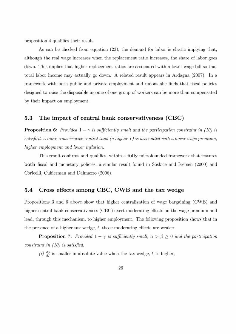
proposition 4 qualifies their result.

As can be checked from equation (23), the demand for labor is elastic implying that,

although the real wage increases when the replacement ratio increases, the share of labor goes

down. This implies that higher replacement ratios are associated with a lower wage bill so that

total labor income may actually go down. A related result appears in Ardagna (2007). In a

framework with both public and private employment and unions she finds that fiscal policies

designed to raise the disposable income of one group of workers can be more than compensated

by their impact on employment.

5.3 The impact of central bank conservativeness (CBC)

Proposition 6: Provided 1− γ is sufficiently small and the participation constraint in (10) is

satisfied, a more conservative central bank (a higher I) is associated with a lower wage premium,

higher employment and lower inflation.

This result confirms and qualifies, within a fully microfounded framework that features

both fiscal and monetary policies, a similar result found in Soskice and Iversen (2000) and

Coricelli, Cukierman and Dalmazzo (2006).

5.4 Cross effects among CBC, CWB and the tax wedge

Propositions 3 and 6 above show that higher centralization of wage bargaining (CWB) and

higher central bank conservativeness (CBC) exert moderating effects on the wage premium and

lead, through this mechanism, to higher employment. The following proposition shows that in

the presence of a higher tax wedge, t, those moderating effects are weaker.

Proposition 7: Provided 1 − γ is sufficiently small, α > β ≥ 0 and the participation

constraint in (10) is satisfied,

(i) dφdIis smaller in absolute value when the tax wedge, t, is higher,

26

(ii) dφ

d( 1n)is smaller in absolute value when the tax wedge, t, is higher.

6 Welfare analysis.

This section evaluates the effects of competitiveness in the goods and labor markets, of fiscal

policy parameters and of CBC on aggregate welfare. We use a Benthamite measure of social

welfare that is based on the sum of the indirect utility functions, bva, of all individuals in thegeneral equilibrium. Total welfare equals the welfare of employed workers plus the welfare of

unemployed workers, each weigthed by its appropriate proportion in the labor force, plus the

welfare of employers. Aggregate welfare is given, therefore, by

bva = ((1− u)vEW + uvUW )L0 + vE. (40)

Substituting (15) into (40) and rearranging

bva = (1 + L0)M

P+

Bu+ χ

PL0 + (1− u)

W

PL0 +RuL0 +

Π

P

= (1 + L0)M

P+

½(1− u)

tW

(1− t)P+ (1− u)

W

P

¾L0 +

Π

P+ uRL0 (41)

where the last equality follows from the government budget constraint in (11) and the reader is

reminded that χ ≡ TRW + 1LoTRE. Gross real income is equal to the sum of (real) taxes, net

wages and profits. Hence

Y =

½(1− u)

tW

(1− t)P+ (1− u)

W

P

¾L0 +

Π

P. (42)

27

Using (42) in (41), average welfare per individual can be expressed as

bv ≡ bva1 + L0

=M

P+

Y +RuL01 + L0

. (43)

It is shown in Appendix 9.6 that bv can be expressed as the following function of the wagepremium:

bv(φ) = Ψ5 · [1− φ]α

1−α +Lα0

1 + L0

∙1− φ

1− α

¸α+

L01 + L0

µφ

1− α

¶·R (44)

where Ψ5 > 0 is defined in equation (102) in the appendix. Inspection of (44) suggests that

except for the elasticity of substitution, θ, the main parameters of interest affect welfare only

through the wage premium, φ. Consequently an important intermediate step in determining the

effects of those parameters on welfare involves finding the effect of the wage premium on bv(φ).An increase in the wage-premium, φ, has three effects on bv(φ): (i) it reduces utility by reducingincome from production, (ii) it increases utility by raising the number of unemployed, so that

their total leisure increases and (iii) it reduces utility by reducing real balances.

Based on (44) we can find how goods’ market competitiveness, CWB, the tax wedge,

the replacement ratio and CBC, affect welfare through φ by totally differentiating bv(φ) withrespect to

¡θ, 1

n, t, β, I

¢. The resulting expressions can then be combined with propositions 2-6

to establish the effect of each of those parameters on welfare. The results are summarized in

the following propositions and demonstrated in Appendix 9.6:

Proposition 8: For (1− γ) sufficiently small,

(i) The higher the replacement ratio, β, the lower social welfare.

If in addition, the participation constraint and the conditions α > β ≥ 0 and

α [(1− u)L0]α−1 > R, (45)

28

are satisfied, then:

(ii) The higher CWB, 1n, the higher social welfare,

(iii) The higher the tax wedge, t, the lower social welfare.

(iv) The higher CBC, I, the higher social welfare.

Condition (45) requires that the marginal contribution to output (and therefore consumption)

from an additional employed individual has to be greater than the value of leisure foregone by

the individual. It is a necessary condition for some positive employment to be socially desirable.

The intuition underlying the results in proposition 8 follows. A higher degree of cen-

tralization of wage bargaining, by raising the degree of internalization of the macroeconomic

impact of its actions, moderates the wage demands of each union, leading to lower real wages,

more employment, higher income and higher welfare. By raising the wage demands of unions

increases in the replacement ratio and the tax wedge lead to higher real wage costs to firms,

higher unemployment, lower aggregate income and lower welfare. Finally, a higher degree of

CBC, by sending a signal to unions that the CB will react to higher wage demands with a

stronger contraction of aggregate demand, moderates their wage demands raising employment,

income and welfare.

7 Fiscal policy and special interests.

To this point, fiscal policy has been taken as exogenous. This section extends the analysis by

adding a first stage during which a political authority picks fiscal instruments, anticipating the

reactions of labor unions, the central bank and price setters in subsequent stages. Formally, the

fiscal authority is modeled as a Stackelberg leader.

It is well known that the motives of political authorities and of social planners are not

fully aligned. Although this does not necessarily mean that politicians do not care at all about

social welfare, it usually implies that they also care about redistribution in favor of particu-

29

lar constituencies. We therefore endow fiscal authorities with an objective function that is a

weighted average of social welfare and of redistribution in favor of particular constituencies. In

particular, government’s objective function is given by:

Υ = δ ·hχPL0i+ (1− δ) · bv (46)

As the discussion preceding equation (11) clarifies the term χPL0 on the right-hand side of (46)

represents the total amount of real transfer payments in favour of preferred constituencies.27

Thus, the parameter δ ∈ [0, 1] represents the weight given by government to redistribution in

favor of "special interests" and 1− δ represents the weight given to, bv - - the indirect utility ofthe average individual in the economy that is given by (44). For simplicity we abstract from

public goods and unemployment benefits by assuming that fiscal policy instruments consist only

of taxation and of lump sum redistribution so that B = β = 0. As a consequence government’s

budget constraint in (11) specializes to

χ

PL0 =

W

P

t(1− u)L01− t

≡ T (t). (47)

The left hand side of (47) represents total real redistribution and the right hand side represents

total real taxes.

The instrument of fiscal policy - - the tax rate t - - is chosen to maximize (46) subject

to the budget constraint in (47). To develop some intuition about the mechanisms underlying

government’s choice it is convenient to start with two extreme particular cases: (i) a government

that has no interest in redistribution (δ = 0) and, (ii) a government that only cares about

redistribution in favour of supporters (δ = 1).

27Since χ ≡ TRW + 1L0TRE is the average transfer per worker in the economy χL0 represent total nominal

transfers. Note that, although transfers aremeasured per worker, they can accomodate any pattern of transfersbetween workers and entrepeneurs.

30

Case (i). A government that only cares about social welfare gives no weight to redistri-

bution (δ = 0) and sets t so as to maximize bv. Part (iii) of proposition 8 implies that welfareis maximized when t = 0. Hence, like a Benthamite social planner, a government with no

redistributional concerns does not impose taxes.28

Case (ii) A totally partisan government that only cares about the special interests of its

preferred constituency (δ = 1) chooses the tax wedge, t, so as to maximize T , the amount of

funds available for redistribution in (47). Formally such a government sets the tax wedge, t, so

that (for an internal solution) the condition dT (t)dt

= 0 is satisfied.29 In general, the derivativedT (t)dtmay be of either sign, since a higher tax rate reduces economic activity. However, a rational

government will never operate on the inefficient side of the Laffer-curve. That is, the equilibrium

value of t must be such that dT (t)dt≥ 0. Further details appear at the end of Appendix 9.6.

7.1 Characterization of t and of the size of government in the general

case

In order to characterize the equilibrium values of t and of total redistribution in this intermediate

case, we need to express all the components of T in (47) as a function of t. Since both the real

wage and unemployment depend on t via the wage premium,we start by expressing T in terms

of the wage premium, φ(t), where the notation highlights the dependence of the wage premium

on the tax wedge. Equation (75) in Appendix 9.3 implies

W

P=

µW

P

¶c

1

(1− φ(t))∼= exp(wg

rc)(1− t)

(1− φ(t)). (48)

28Obviously, this extreme conclusion is a consequence of the implicit assumption that utility from public goodsis zero. In the presence of utilty from public goods there will be, in this case, some taxation but only to financethe public good.29As pointed out by Meltzer and Richard (1981) such a political equilibrium arises when the median voter in

their model does not work.

31

Inserting (32) and (48) into the middle expression in (47), rearranging and inserting the resulting

expression into (46) the objective function of the fiscal authority can be expressed as the following

function of t

Υ(t) = δ · T + (1− δ) · bv ∼= δ exp(wgrc)

t · L0(1− φ(t))

∙1− φ(t)

1− α

¸+ (1− δ)bv(t). (49)

For an internal solution the tax rate, t∗, that maximizes government’s objectives in (49) has to

satisfy the first-order condition

dΥ(t∗)

dt= δ

dT (t∗)

dt+ (1− δ)

dbv(φ(t∗))dφ

dφ

dt= 0 (50)

where the functions T (t) and bv(t) are given by (47) and (44) respectively. Part (iii) of proposition8 implies that dv(φ(t∗))

dφ< 0 and, from proposition 4, dφ

dt> 0. Hence the second term on the

right hand side of (50) is negative. It follows that dT (t∗)dt

> 0. This confirms that government

operates on the efficient side of the Laffer curve also in the intermediate case. It implies that

the equilibrium size of redistribution (and therefore of government) is an increasing function of

the tax wedge.

7.2 Comparative statics, CBC and the size of government

Application of the implicit function theorem to (50) yields

dt∗

dδ= −

dT (t∗)dt− dv(φ(t∗))

dφdφdt

SOC(t∗)

where SOC(t∗) < 0 is the second order condition for government’s decision problem. Proposition

4 and part (iii) of proposition 8 imply that dT (t∗)dt− dv(φ(t∗))

dφdφdt

> 0. This leads to the following

proposition.

32

Proposition 9: Governments with higher relative distributional concerns (higher δ0s)

set higher tax wedges and are larger.

The impact of CBC on the tax policy of Government is generally ambiguous since an

increase in CBC triggers two opposing effects on the marginal impact of the tax wedge on total

tax collections and redistribution. On one hand, by raising dTdtfor a given wage premium, an

increase in I tends to increase the revenue enhancing marginal impact of t on tax collections.

This effect encourages Government to raise the tax wedge. On the other hand, higher CBC,

by magnifying the adverse effect of t on the wage premium and unemployment operates in

the opposite direction.30 The following proposition (demonstrated in Appendix 9.6) provides a

sufficient condition for the dominance of the first effect.

Proposition 10: Provided the cross-derivative, d2φdt·dI , is not too large, the tax rate, t

∗, set by

fiscal autorities is increasing in the level of CBC, I.

7.3 An implication for the social desirability of strict inflation tar-

geting

An implication of proposition 10 is that, when the effect of CBC on the (now endogenously

determined) tax wedge is taken into consideration, the optimal long run level of conservativeness

may no longer be infinite. The reason is that although, given the tax wedge, an ultra conservative

CB is optimal (by part (iv) of proposition 8) it may induce government to raise the tax wedge

which (by part (iii) of proposition 8) reduces welfare. The upshot is that, when the impact

of conservativeness on welfare through the choice of tax wedge by government is taken into

consideration, an ultra conservative CB, or equivalently - - a strict inflation targeter - - may no

longer be optimal. An analytical formulation of this point appears in Appendix 9.7

30A higher I also triggers two opposing effects on the marginal impact of t on welfare.

33

8 Concluding remarks

This paper explores the implications of interactions between fiscal policy and monetary policy-

making institutions in an economy with imperfectly competitive labor and goods markets with

sticky wages and flexible prices. Such a framework appears to be a more realistic description

of economic realities in Europe than some New Keynesian models featuring a competitive labor

market with sticky prices and flexible wages for at least two reasons. First, and most obviously,

the labor force in Europe is largely unionized. Second, recent evidence from the ECB inflation

network supports the view that wages are stickier than prices.

As emphasized by Soskice and Iversen (2000) and Coricelli, Cukierman and Dalmazzo

(2006) and others, one basic difference between a competitive labor market and a labor market

characterized by large wage setters is that in the latter case, due to the fact that unions inter-

nalize the response of the central bank (CB) to their wage setting decisions, the level of CBC

affects unemployment and other real variables even in the long run. A basic consequence of this

"strategic effect" is that, in the absence of shocks (and therefore no benefit from stabilization

policy) strict inflation targeting improves performance not only on the inflation front but it also

reduces unemployment and is therefore socially optimal.

The result above is obtained within frameworks that abstract from fiscal policy. This

paper discusses the impact of fiscal policy decisions on this mechanism, as well as on the reverse

causality from CBC to the choice of fiscal policy variables like labor taxes and redistribution.

Two results stand out in this context. First, as long as labor taxes and unemployment ben-

efits are given exogenously the social desirability of strict inflation targeting is robust to the

introduction of fiscal policy. However, higher conservativeness on the part of the CB often in-

duces governments with redistributional concerns to raise taxes, and this reduces social welfare.

As a consequence flexible inflation targeting may be socially optimal even in the absence of

34

stabilization policy.31

We use the framework of the paper to investigate the impact of economic structure, fiscal

policy, central bank conservativeness (CBC), and their interactions on economic performance in

the long run. A central determinant of economic performance in our model is the wage premium

- - defined as the percentage (upward) deviation of the equilibrium real wage in the presence of

unions from its counterpart when the labor market is competitive. The paper investigates the

long run impact of labor taxes, the replacement ratio, goods market competitiveness, central-

ization of wage bargaining and CBC on the wage premium, and through it, on unemployment,

inflation and related macroeconomic variables. Under reasonable restrictions higher values of the

tax wedge and of the replacement ratio are associated with a higher wage premium, while higher

values of centralization of wage bargaining and of CBC are associated with a lower premium.

Social welfare, defined as the sum of all individual utilities, is negatively related to the

wage premium. As a consequence higher values of the tax wedge and of the replacement ratio

are associated with lower welfare. By contrast higher values of good market competitiveness, of

centralization of wage bargaining and of CBC are associated with higher welfare.

Blanchard and Giavazzi (2003) note that since the end of the seventies there has been

a persistent decline in labor share and a persistent increase in the rate of unemployment in

Germany, France, Italy and Spain. Our model predicts that increases in labor taxes should

cause both of those developments. It is therefore interesting to examine what happened to those

taxes in Europe since the end of the seventies. Table 1 in Ardagna (2007) suggests that (for a

sample of ten European countries that includes the four countries above) the average effective

tax rate on labor income has risen from about 32% in the mid seventies to almost 43% during

the first half of the nineties.32

31By contrast in Rogoff (1985) classic framework, since CBC does not affect employment in the long run, astrict inflation targeter is socially optimal in the absence of stabilization policy.32Blanchard and Giavazzi (2003) explore an alternative hypothesis that relies on changes in the bargaining

power of labor.

35

Finally, one intriguing consequence of our framework is that the share of labor in the

presence of unions is lower than this share when the labor market is competitive. Furthermore,

this share is a decreasing function of the wage premium.

9 Appendix.

9.1 The individual consumer’s problem.

Omitting, without loss of generality, the class index, c, and using the first-order conditions with

respect to varieties j and s, we obtain

Cj

Cs=

µPj

Ps

¶−θ, for any (j, s). (51)

Solving for Cj from (51), substituting it into (4) and using (3), we obtain

Cj =

µPj

P

¶−θ µA−M

P

¶. (52)

Raising both sides of (52) to power¡θ−1θ

¢, integrating over j and raising the result to power¡

θθ−1¢, one also obtains that C = A−M

P. Hence

Cj =

µPj

P

¶−θC. (53)

Combining the first-order conditions with respect to variety j and money,M , we obtainγC− 1θ

j

Cθ−1θ

=

(1−γ)PjM

. Using (53) to substitute Cj out from this expression and rearranging

C =γ

1− γ

µM

P

¶. (54)

36

Each individual’s demand for variety j, given by (51), can therefore be rewritten as

Cj =

µPj

P

¶−θ µγ

1− γ

¶µM

P

¶. (55)

The demand for nominal money (equation (13) in the text) is obtained by substituting this

expression for Cj in the individual’s budget constraint (4) and by rearranging. Substituting

(13) into (54), the consumption aggregator, C, can be expressed as

C = γA

P. (56)

Similarly, using (13), we can rewrite (55) as

Cj = γ

µPj

P

¶−θ µA

P

¶. (57)

As demonstrated later, in a symmetric equilibrium individual behavior differs only among three

classes of individuals: employed workers, unemployed workers and employers. Aggregating (57)

over the mass of individuals in the economy and using equations (4) and (5), total demand for

variety j is given by

Caj = γ

µPj

P

¶−θAa

P= γ

µPj

P

¶−θ ∙(1 + L0)

M

P+ Y

¸. (58)

The expression for total demand for variety j in equation (20) of the text is obtained by inserting

(19) into (58) above and by rearranging. Finally, the indirect utility function in equation (14)

in the text is obtained by substituting (13) and (56) into the utility function (1).

37

9.2 Derivation of expressions for inflation, unemployment and the

Central Bank’s reaction function

To derive the reaction function of the CB we have to express inflation and unemployment in

terms of the money supply. To obtain an expression for inflation we raise the equilibrium relative

price of each firm in (22) to the power of (1− θ) and integrate over firms. Using (3) and taking

natural logarithms of the resulting expression we obtain:

0 = logΨ1 +1− α

D(m− p) +

α

D(τ − p) +

1

1− θlog

µZ 1

0

Wα(1−θ)

Dj dj

¶(59)

where τ ≡ − log(1 − t), and m and p denote the natural logarithms of M and P respectively,

and Ψ1 ≡∙

θ(θ−1)α

³γ(1+L0)1−γ

´ 1−αα

¸ αD

. The price-level, p, is obtained by rearranging (59) and by

substituting it into the definition of inflation.

To obtain the rate of unemployment, u, we aggregate (23) over firms and take logs.

Defining log(L0) ≡ l0, we obtain:

u ≡ l0 − ld = [l0 − logΨ2]−1

D(m− p)− θ

D(p− τ)− log

µZ 1

0

W−θDj dj

¶(60)

where Ψ2 ≡³

θ(θ−1)α

´− θD³γ(1+L0)1−γ

´ 1D. Equation (25) in the text is obtained by using (24) to

substitute out p = π + p−1 in (60). Substituting (24) and (25) into (8), the Central Bank’s

objective function can be rewritten as:

Γ =n[l0 − logΨ2 + (1− θ) logΨ1]−m+ τ + log

³cW1

´− log

³cW2

´o2+

+I ·½[D logΨ1] + (1− α)m+ ατ +

D

1− θlog³cW1

´− p−1

¾2(61)

The reaction function in equation (26) in the text is obtained by maximizing (61) with respect

38

to m. The constant, Ψm, is given by

Ψm ≡l0 − logΨ2 + [(1− θ)− (1− α)ID] logΨ2 + (1− α)Ip−1

1 + (1− α)2I

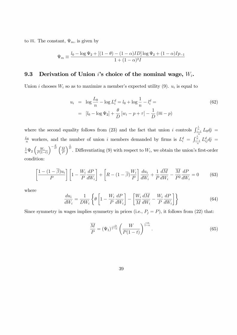
9.3 Derivation of Union i’s choice of the nominal wage, Wi.

Union i chooses Wi so as to maximize a member’s expected utility (9). ui is equal to

ui = logL0n− logLd

i = l0 + log1

n− ldi = (62)

= [l0 − logΨ2] +θ

D[wi − p+ τ ]− 1

D(m− p)

where the second equality follows from (23) and the fact that union i controlsR i

ni−1n

L0dj =

L0nworkers, and the number of union i members demanded by firms is Ld

i =R i

ni−1n

Ldijdj =

1nΨ2

³Wi

P (1−t)

´− θD³MP

´ 1D. Differentiating (9) with respect toWi, we obtain the union’s first-order

condition:

∙1− (1− β)ui

P

¸ ∙1− Wi

P

dP

dWi

¸+

∙R− (1− β)

Wi

P

¸duidWi

+1

P

dM

dWi− M

P 2dP

dWi= 0 (63)

whereduidWi

=1

DWi

½θ

∙1− Wi

P

dP

dWi

¸−∙Wi

M

dM

dWi− Wi

P

dP

dWi

¸¾(64)

Since symmetry in wages implies symmetry in prices (i.e., Pj = P ), it follows from (22) that:

M

P= (Ψ1)

−D1−α

µW

P (1− t)

¶ −α1−α

. (65)

39

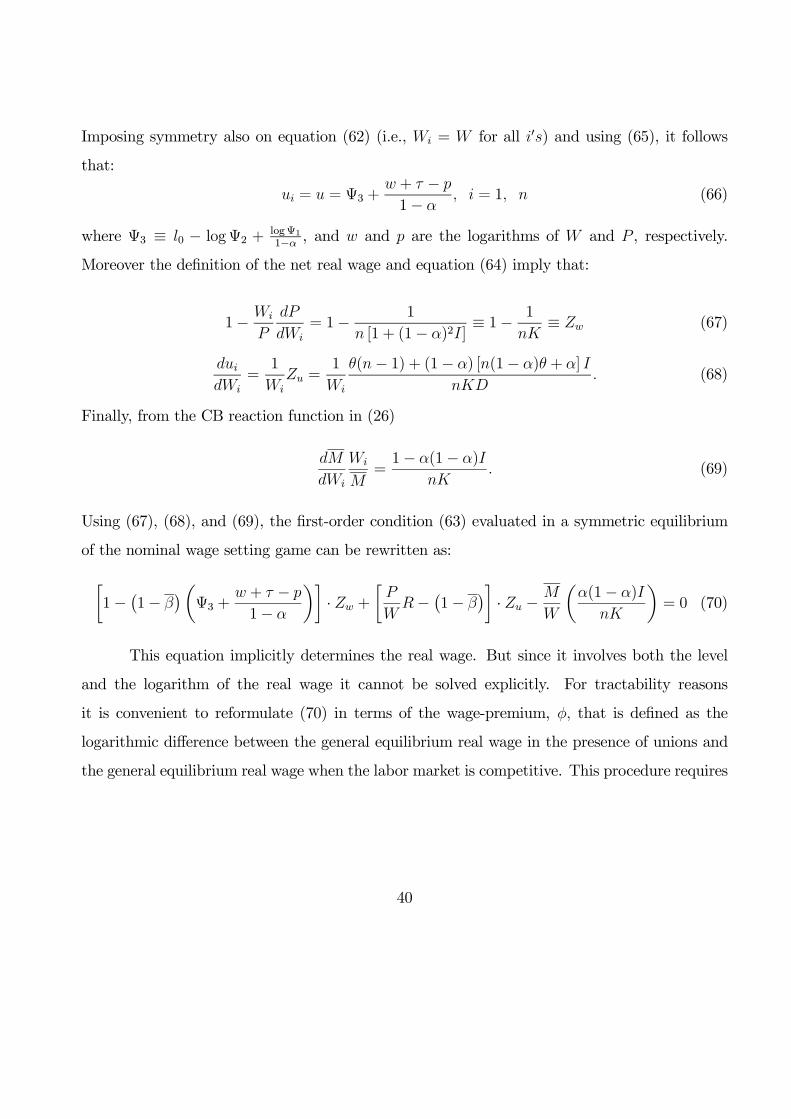
Imposing symmetry also on equation (62) (i.e., Wi = W for all i0s) and using (65), it follows

that:

ui = u = Ψ3 +w + τ − p

1− α, i = 1, n (66)

where Ψ3 ≡ l0 − logΨ2 +logΨ11−α , and w and p are the logarithms of W and P , respectively.

Moreover the definition of the net real wage and equation (64) imply that:

1− Wi

P

dP

dWi= 1− 1

n [1 + (1− α)2I]≡ 1− 1

nK≡ Zw (67)

duidWi

=1

WiZu =

1

Wi

θ(n− 1) + (1− α) [n(1− α)θ + α] I

nKD. (68)

Finally, from the CB reaction function in (26)

dM

dWi

Wi

M=1− α(1− α)I

nK. (69)

Using (67), (68), and (69), the first-order condition (63) evaluated in a symmetric equilibrium

of the nominal wage setting game can be rewritten as:

∙1−

¡1− β

¢µΨ3 +

w + τ − p

1− α

¶¸· Zw +

∙P

WR−

¡1− β

¢¸· Zu −

M

W

µα(1− α)I

nK

¶= 0 (70)

This equation implicitly determines the real wage. But since it involves both the level

and the logarithm of the real wage it cannot be solved explicitly. For tractability reasons

it is convenient to reformulate (70) in terms of the wage-premium, φ, that is defined as the

logarithmic difference between the general equilibrium real wage in the presence of unions and

the general equilibrium real wage when the labor market is competitive. This procedure requires

40

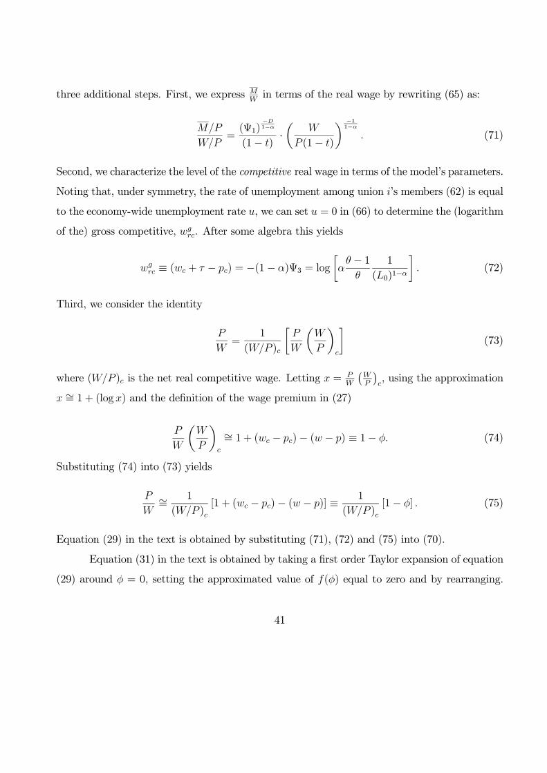
three additional steps. First, we express MWin terms of the real wage by rewriting (65) as:

M/P

W/P=(Ψ1)

−D1−α

(1− t)·µ

W

P (1− t)

¶ −11−α

. (71)

Second, we characterize the level of the competitive real wage in terms of the model’s parameters.

Noting that, under symmetry, the rate of unemployment among union i’s members (62) is equal

to the economy-wide unemployment rate u, we can set u = 0 in (66) to determine the (logarithm

of the) gross competitive, wgrc. After some algebra this yields

wgrc ≡ (wc + τ − pc) = −(1− α)Ψ3 = log

∙αθ − 1θ

1

(L0)1−α

¸. (72)

Third, we consider the identity

P

W=

1

(W/P )c

∙P

W

µW

P

¶c

¸(73)

where (W/P )c is the net real competitive wage. Letting x = PW

¡WP

¢c, using the approximation

x ∼= 1 + (log x) and the definition of the wage premium in (27)

P

W

µW

P

¶c

∼= 1 + (wc − pc)− (w − p) ≡ 1− φ. (74)

Substituting (74) into (73) yields

P

W∼= 1

(W/P )c[1 + (wc − pc)− (w − p)] ≡ 1

(W/P )c[1− φ] . (75)

Equation (29) in the text is obtained by substituting (71), (72) and (75) into (70).

Equation (31) in the text is obtained by taking a first order Taylor expansion of equation

(29) around φ = 0, setting the approximated value of f(φ) equal to zero and by rearranging.

41

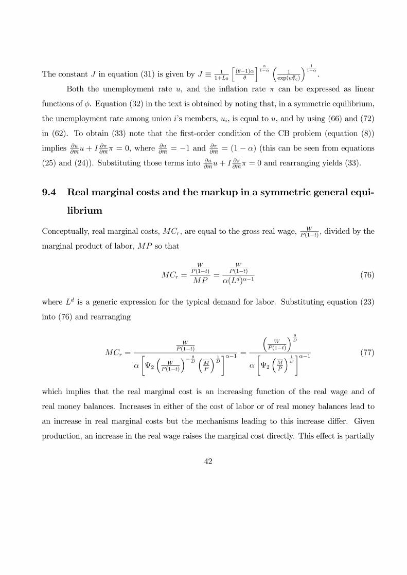
The constant J in equation (31) is given by J ≡ 11+L0

h(θ−1)α

θ

i α1−α³

1exp(wgrc)

´ 11−α.

Both the unemployment rate u, and the inflation rate π can be expressed as linear

functions of φ. Equation (32) in the text is obtained by noting that, in a symmetric equilibrium,

the unemployment rate among union i’s members, ui, is equal to u, and by using (66) and (72)

in (62). To obtain (33) note that the first-order condition of the CB problem (equation (8))

implies ∂u∂m

u + I ∂π∂m

π = 0, where ∂u∂m= −1 and ∂π

∂m= (1 − α) (this can be seen from equations

(25) and (24)). Substituting those terms into ∂u∂m

u+ I ∂π∂m

π = 0 and rearranging yields (33).

9.4 Real marginal costs and the markup in a symmetric general equi-

librium

Conceptually, real marginal costs, MCr, are equal to the gross real wage, WP (1−t) , divided by the

marginal product of labor, MP so that

MCr =

WP (1−t)

MP=

WP (1−t)

α(Ld)α−1(76)

where Ld is a generic expression for the typical demand for labor. Substituting equation (23)

into (76) and rearranging

MCr =

WP (1−t)

α

∙Ψ2

³W

P (1−t)

´− θD³MP

´ 1D

¸α−1 =³

WP (1−t)

´ θD

α

∙Ψ2³MP

´ 1D

¸α−1 (77)

which implies that the real marginal cost is an increasing function of the real wage and of

real money balances. Increases in either of the cost of labor or of real money balances lead to

an increase in real marginal costs but the mechanisms leading to this increase differ. Given

production, an increase in the real wage raises the marginal cost directly. This effect is partially

42

offset through the fact that the firm cuts production - which raises the marginal product of

labor and reduces marginal costs. But, the extreme right hand side of (77) suggests that the

direct effect dominates so that the overall effect of an increase in the real wage is to increase

marginal costs. When real money balances (and therefore demand) increase, the firm responds

by expanding production so that, given the decreasing marginal productivity of labor, marginal

costs increase.

But this intuitive account of the economic forces at work abstracts from an additional

general equilibrium relation between real balances and the gross real wage that is summarized

by equation (65) of the appendix. That relation arises because, when the gross real wage rises,

all firms try to raise their relative prices. Since they all do that by raising their nominal prices,

none of them manages to increase its relative price. But their joint attempt to raise their

relative prices leads to an increase in the general price level which, given the nominal money

supply, depresses real money balances and with it aggregate demand. The upshot is that there

is a general equilibrium inverse relation between real money balances and the gross real wage.

Taken alone, this additional channel leads to a decrease in aggregate demand and production

so that marginal costs decrease.

It turns out that for the Blanchard-Kiyotaki-Fischer-Dixit-Stiglitz (BKFDS) framework

that underlies the structure of demand in our model (as well as in many other contemporary

models with monopolistic competition) the downward effect of a change in the real wage through

demand exactly offsets its upward effect on marginal costs through supply. This can be seen

by substituting equation (65) from the appendix into (77). After cancellation of terms and

rearrangement, this yields equation (38) in the text implying that in a symmetric general equi-

librium marginal costs depend only on the elasticity of substitution, θ. Although this result is

due to the specific form of the BKFDS framework it can serve as a useful benchmark.

We turn next to the calculation of the markup in a symmetric general equilibrium. The

43

markup, µ, is defined as the real equilibrium price divided by the real marginal cost33

µ ≡PjP

MCr=

1

MCr=

θ

θ − 1 . (78)

Thus, in a symmetric general equilibrium, real marginal costs and the markup are fully deter-

mined by the degree of competitiveness in the goods markets as characterized by the elasticity

of substitution, θ. Equation (78) is a familiar expression for the markup in many other models

of monopolistic competition based on a Dixit-Stiglitz utility with competitive labor markets.

This analysis suggests that, at least for BKFDS type frameworks, the expression for the long

run markup is invariant to the structure and degree of competitiveness of labor markets.

9.5 Proofs of propositions 2-7

The derivations of the impacts on the wage premium are obtained by differentiating the ex-

pression for the wage premium in equation (31) with respect to the appropriate structural or

fiscal policy variable and by using the additional constraints specified in each proposition. The

impacts on unemployment and inflation are inferred from equations (32) and (33). In estab-

lishing the impact of a given structural or fiscal policy variable s, s = θ, 1n, t, β, I, some similar

expressions appear. Those expressions are derived once in the early stages of the proof and used

subsequently, as appropriate, to complete the proof of each separate proposition. It is convenient

to rewrite (31) as

φ ∼=N1 −

³1−γγ

´N2

D1 −³1−γγ

´D2

(79)

33The second equality in (78) follows from the fact that all firms set the same price in a symmetric equilibrium.

44

where

N1 ≡Zw

Zu+

R

(1− t) exp(wgrc)− (1− β), N2 ≡

α (1− α) I

nKZu

µJ

1− t

¶D1 ≡

µ1− β

1− α

¶Zw

Zu+

R

(1− t) exp(wgrc)

, D2 ≡αI

nKZu

µJ

1− t

¶. (80)

Differentiating φ with respect to the dummy index, s, and rearranging

dφ

ds∼=

D1dN1ds−N1

dD1

ds+ 1−γ

γQ³

D1 −³1−γγ

´D2

´2 (81)

where

Q ≡µ1− γ

γD2 −D1

¶dN2

ds−µ1− γ

γN2 −N1

¶dD2

ds+N2

dD1

ds−D2

dN1

ds(82)

Under the assumption that 1−γγis relatively small an approximate expression for the impact of

s on the wage premium isdφ

ds∼=

D1dN1ds−N1

dD1

ds

D21

(83)

Proof of proposition 2:

(i) From equation (28),

wgrc = log

∙αθ − 1θ

1

(L0)1−α

¸. (84)

Hence the net competitive real wage is given by

µW

P

¶c

= (1− t)

µαθ − 1θ

1

(L0)1−α

¶. (85)

Inspection of this equation reveals that

d¡WP

¢c

dθ> 0. (86)

45

(ii) Using (80), (30) and (28) to evaluate (83) for s = θ, and rearranging,

dφ

dθ=

d(ZwZw )dθ

(1−β)(1−α)(WP )c

n(1− β)

¡WP

¢c− α−β

1−βRo− d(WP )c

dθR

(1−t)(WP )2

c

nh(1−β)(1−α) − 1

iZwZw+ (1− β)

oD21

(87)

Lemma 1:d(ZwZw )dθ

< 0.

Proof: From (30), ZwZudepends on θ only through Zu and Zu depends on θ only through the

term θD. It suffices therefore to show that

d( θD )dθ

> 0. Butd( θD )dθ

= αD2 > 0. QED.

Lemma 2: The participation constraint implies (1− β)¡WP

¢c− α−β

1−βR > 0.

Proof: Using equation (15) in (10), the participation constraint can be rewritten as

µW

P

¶c

> β

µW

P

¶c

+R (88)

or

β +R¡WP

¢c

≡ β + r < 1. (89)

Simple algebra shows that the statement of the Lemma is equivalent to

β +α− β

1− βr < 1. (90)

Hence, it suffices to establish the inequality in (90). The proof of the Lemma is completed by

noting that, since α < 1, the participation constraint in (89) implies (90).

Consider now the numerator of equation (87). The fact that both α and β are bounded

between zero and one in conjunction with Lemmas 1 and 2 imply that the first term in the

numerator is negative. Equation (86) and the condition α > β, imply that the second term in

the numerator is negative as well. It follows that dφdθ

< 0.

The impacts on unemployment and inflation follow directly from equations (32) and (33).

46

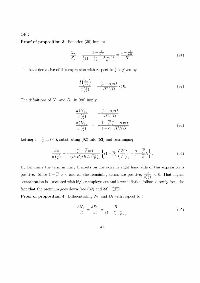
QED

Proof of proposition 3: Equation (30) implies

Zw

Zu=

1− 1nK

θD(1− 1

n) + (1−α)I

K1n

≡1− 1

nK

H. (91)

The total derivative of this expression with respect to 1nis given by

d³ZwZu

´d¡1n

¢ = −(1− α)αI

H2KD< 0. (92)

The definitions of N1 and D1 in (80) imply

d (N1 )

d¡1n

¢ = −(1− α)αI

H2KD

d (D1 )

d¡1n

¢ = −1− β

1− α

(1− α)αI

H2KD(93)

Letting s = 1nin (83), substituting (92) into (83) and rearranging

dφ

d¡1n

¢ = − (1− β)αI

(D1H)2KD¡WP

¢c

½(1− β)

µW

P

¶c

− α− β

1− βR

¾. (94)

By Lemma 2 the term in curly brackets on the extreme right hand side of this expression is

positive. Since 1 − β > 0 and all the remaining terms are positive, dφ

d( 1n)< 0. That higher

centralization is associated with higher employment and lower inflation follows directly from the

fact that the premium goes down (see (32) and 33). QED

Proof of proposition 4: Differentiating N1 and D1 with respect to t

dN1

dt=

dD1

dt=

R

(1− t)¡WP

¢c

. (95)

47

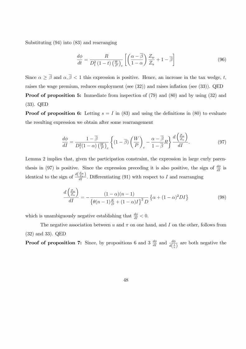
Substituting (94) into (83) and rearranging

dφ

dt=

R

D21 (1− t)

¡WP

¢c

∙µα− β

1− α

¶Zw

Zu+ 1− β

¸(96)

Since α ≥ β and α, β < 1 this expression is positive. Hence, an increase in the tax wedge, t,

raises the wage premium, reduces employment (see (32)) and raises inflation (see (33)). QED

Proof of proposition 5: Immediate from inspection of (79) and (80) and by using (32) and

(33). QED

Proof of proposition 6: Letting s = I in (83) and using the definitions in (80) to evaluate

the resulting expression we obtain after some rearrangement

dφ

dI=

1− β

D21(1− α)

¡WP

¢c

½(1− β)

µW

P

¶c

− α− β

1− βR

¾ d³ZwZu

´dI

. (97)

Lemma 2 implies that, given the participation constraint, the expression in large curly paren-

thesis in (97) is positive. Since the expression preceding it is also positive, the sign of dφdIis

identical to the sign ofd(ZwZu )dI

. Differentiating (91) with respect to I and rearranging

d³ZwZu

´dI

= − (1− α)(n− 1)©θ(n− 1)K

D+ (1− α)I

ª2D

©α+ (1− α)2DI

ª(98)

which is unambiguously negative establishing that dφdI

< 0.

The negative association between u and π on one hand, and I on the other, follows from

(32) and 33). QED

Proof of proposition 7: Since, by propositions 6 and 3 dφdIand dφ

d( 1n)are both negative the

48

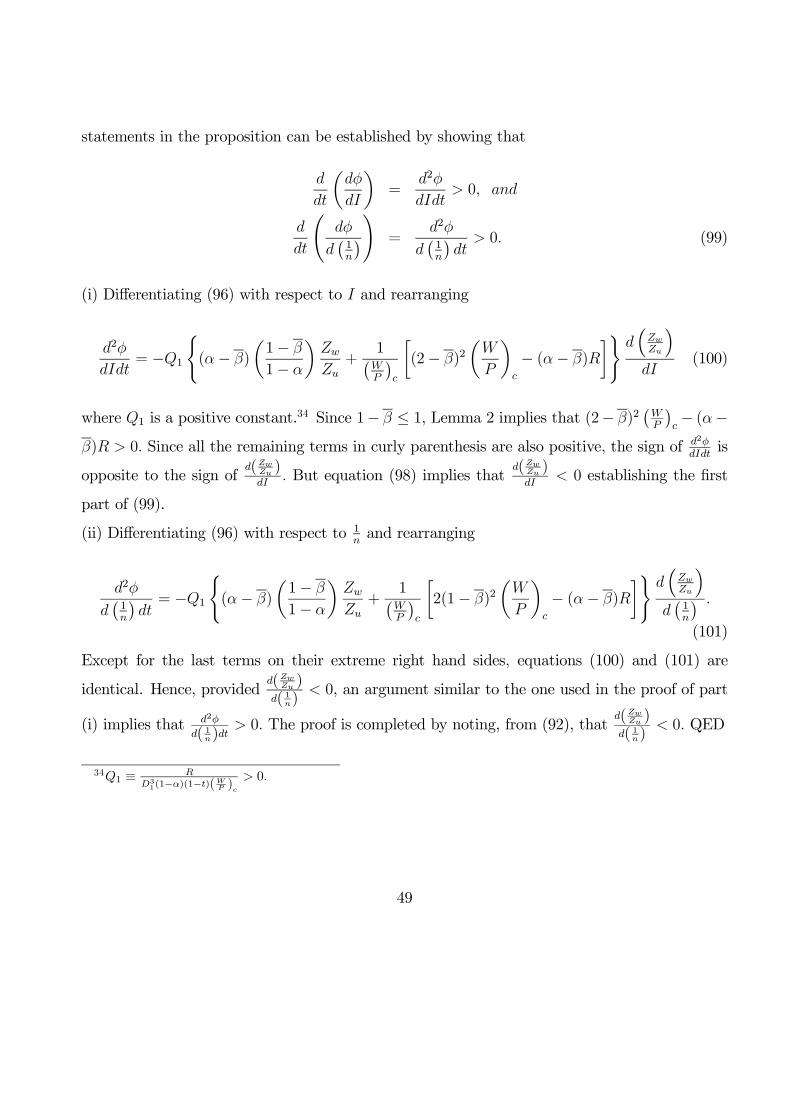
statements in the proposition can be established by showing that

d

dt

µdφ

dI

¶=

d2φ

dIdt> 0, and

d

dt

Ãdφ

d¡1n

¢! =d2φ

d¡1n

¢dt

> 0. (99)

(i) Differentiating (96) with respect to I and rearranging

d2φ

dIdt= −Q1

((α− β)

µ1− β

1− α

¶Zw

Zu+

1¡WP

¢c

∙(2− β)2

µW

P

¶c

− (α− β)R

¸) d³ZwZu

´dI

(100)

where Q1 is a positive constant.34 Since 1− β ≤ 1, Lemma 2 implies that (2− β)2¡WP

¢c− (α−

β)R > 0. Since all the remaining terms in curly parenthesis are also positive, the sign of d2φdIdt

is

opposite to the sign ofd(ZwZu )dI

. But equation (98) implies thatd(ZwZu )dI

< 0 establishing the first

part of (99).

(ii) Differentiating (96) with respect to 1nand rearranging

d2φ

d¡1n

¢dt= −Q1

((α− β)

µ1− β

1− α

¶Zw

Zu+

1¡WP

¢c

∙2(1− β)2

µW

P

¶c

− (α− β)R

¸) d³ZwZu

´d¡1n

¢ .

(101)

Except for the last terms on their extreme right hand sides, equations (100) and (101) are

identical. Hence, providedd(ZwZu )d( 1n)

< 0, an argument similar to the one used in the proof of part

(i) implies that d2φ

d( 1n)dt> 0. The proof is completed by noting, from (92), that

d(ZwZu )d( 1n)

< 0. QED

34Q1 ≡ RD31(1−α)(1−t)(WP )c

> 0.

49

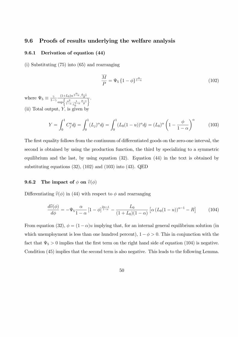
9.6 Proofs of results underlying the welfare analysis

9.6.1 Derivation of equation (44)

(i) Substituting (75) into (65) and rearranging

M

P= Ψ5 {1− φ}

α1−α (102)

where Ψ5 ≡ γ1−γ

(1+L0)αα

1−α . θ−1θ

exp α2

1−α1

L1−α0

θ−1θ

.

(ii) Total output, Y, is given by

Y =

Z 1

0

Caj dj =

Z 1

0

(Lj)αdj =

Z 1

0

(L0(1− u))αdj = (L0)α

µ1− φ

1− α

¶α

(103)

The first equality follows from the continuum of differentiated goods on the zero-one interval, the

second is obtained by using the production function, the third by specializing to a symmetric

equilibrium and the last, by using equation (32). Equation (44) in the text is obtained by

substituting equations (32), (102) and (103) into (43). QED

9.6.2 The impact of φ on bv(φ)Differentiating bv(φ) in (44) with respect to φ and rearranging

dbv(φ)dφ

= −Ψ5α

1− α[1− φ]

2α−11−α − L0

(1 + L0)(1− α)

£α (L0(1− u))α−1 −R

¤(104)

From equation (32), φ = (1−α)u implying that, for an internal general equilibrium solution (in

which unemployment is less than one hundred percent), 1−φ > 0. This in conjunction with the

fact that Ψ5 > 0 implies that the first term on the right hand side of equation (104) is negative.

Condition (45) implies that the second term is also negative. This leads to the following Lemma.

50

Lemma 3: dv(φ)dφ

< 0

9.6.3 Proof of proposition 8

Inspection of equation (44) suggests that each of the parameters 1n, t, β, I affects welfare only

through its effect on the wage premium, φ. Hence

dbv(φ)ds

=dbv(φ)dφ

dφ

ds, s =

1

n, t, β, I. (105)

Since, by Lemma 3, dv(φ)dφ

< 0 the signs of dv(φ)ds

, s = 1n, t, β, I are determined by, and opposite, to

the signs of dφds. The proof of the proposition follows by noting that the signs of dv(φ)

ds, s = 1

n, t, β, I

are given, under the appropriate restrictions (carried over to this proposition) in propositions

3-6. QED

9.7 Government’s choice of tax rate and proof of proposition 10

We start with some preliminaries. Differentiating T in (47) with respect to t,

dT

dt=

W grcL0

1− α

∙1− α− φ

(1− φ)− α · t(1− φ)2

µdφ

dt

¶¸(106)

where W grc = exp(−(1 − α)Ψ3) ≡ Ψ4 is the gross competitive real wage. Differentiating (106)

with respect to I,

d2T

dt · dI ≡ H1 =αΨ4L0

(1− α) (1− φ)2

½µ−dφdI

¶ ∙1 +

2t

(1− φ)

dφ

dt

¸− t

µd2φ

dt · dI

¶¾. (107)

Since, from proposition 4, dφdt

> 0 the first term in curly parenthesis is positive. From part (i) of

proposition 7, d2φdt·dI > 0. Hence the second term in curly parenthesis is negative. It follows that

the sign of (107) is positive whenever d2φdt·dI is not too large.

51

Government’s choice of tax rate and comparative statics on t∗. The tax rate, t∗, is

implicitly determined by equation (50) in the text, where dTdtis given by (106) and dv

dt, obtained

by letting s = t in (105), reduces to:

dbvdt=

dbvdφ× dφ

dt=−L0

£α [L0(1− u)]α−1 −R

¤(1 + L0)(1− α)

× dφ

dt(108)

provided (1−γ) is sufficiently small. Differentiating the expression for dvdφin (108), with respect

to I

d2bvdIdφ

=d

dI

"−L0

£α [L0(1− u)]α−1 −R

¤(1 + L0)(1− α)

#=

∙−αLα

0 (1− u)α−2

(1 + L0)(1− α)

¸× dφ

dI> 0. (109)

Differentiating (108) with respect to I

d2bvdI · dt ≡ H2 =

d2bvdI · dφ ×

dφ

dt+

dbvdφ× d2φ

dI · dt (110)

From (109) and since dφdt

> 0, the first term on the r.h.s. of (110) is positive while the second

one is negative, since dvdφ

< 0 and d2φdI·dt > 0.

From the implicit function theorem, dt∗

dI=

d2ΥdI·dt

− d2Υdt2

. Hence, the sign of dt∗

dIis equal to the

sign of d2ΥdI·dt = δ ·H1+(1− δ) ·H2, where H1 is given by (107), and that of H2 is given by (110).

As we saw above both H1 and H2 are positive when the cross-derivatived2φdIdt

is sufficiently small.

Hence, provided the (positive) cross derivative, d2φdIdt

, is sufficiently small, dt∗

dI> 0 establishing

proposition 10. QED

52

9.8 The socially optimal level of conservativeness when fiscal policy

is endogenous

Since welfare depends on CBC only via the wage premium and since dvdφ

< 0, the level of I that

minimizes the wage premium φ also maximizes welfare. Setting β = 0 and (1− γ) ∼= 0 in (31),

the total derivative of φ with respect to I can be written as:

dφ

dI=

bK1− α

⎡⎣"1− αR¡WP

¢c

#d³ZwZu

´dI

+R

(1− t)¡WP

¢c

∙(1− α) + α

Zw

Zu

¸dt∗(I)

dI

⎤⎦ (111)

where bK is a positive constant, and∙1− α R

(WP )c

¸> 0 by the participation constraint as formu-

lated in equation (88). Sinced(ZwZu )dI

< 0, inspection of the right-hand side of (111) reveals that,

when dt∗(I)dI≤ 0, dφ

dIis uniformly negative implying that an ultra-conservative central banker is

socially optimal . In this case, the solution for CBC is at a corner and I∗ = +∞, as was the

case when fiscal policy was exogenous.

By contrast, when dt∗(I)dI

> 0, the socially optimal level of conservativeness possesses an

internal solution and I∗ <∞. This follows from the fact that limI→∞

µd(ZwZu )dI

¶= 0.

10 References

Alesina A. and R. Perotti (1997), ”The Welfare State and Competitiveness”, American Eco-

nomic Review, 87, 921-39.

Ardagna S. (2007), "Fiscal Policy in Unionized Labor Markets", Journal of Economic

Dynamics and Control, 31, 1498-1534.

Belot M. and J. van Ours (2001), ”Unemployment and Labor Market Institutions. An

Empirical Analysis”, Journal of the Japanese and International Economies, 15, 403-18.

53

Bertola G. (2004), "A Pure Theory of Job Security and Labor Income Risk," Review

of Economic Studies, 71, 43-61.

Blanchard O. and S. Fischer (1988), Lectures on Macroeconomics, The MIT Press,

Canbridge, MA.

Blanchard O. and F. Giavazzi, (2003) "Macroeconomic Effects of Regulation and Deregu-

lation in Goods and Labor Markets",Quarterly Journal of Economics, 118, 879-907, August

Blanchard O. and N. Kiyotaki (1987), "Monopolistic Competition and the Effects of

Aggregate Demand", American Economic Review, 77, 647-676, September.

Clarida R., J. Gali and M. Gertler (1999) "The Science of Monetary Policy: A New-

Keynesian Perspective", Journal of Economic Literature, 37, 1661-1707.

Coricelli F., A. Cukierman and A. Dalmazzo, (2006) "Monetary Institutions, Monop-

olistic Competition, Unionized Labor Markets and Economic Performance", Scandinavian

Journal of Economics, 108, 39-63, March.

Cukierman A. and A. Dalmazzo (2006), "Fiscal-Monetary Policy Interactions in the

Presence of Unionized Labor Markets", International Tax and Public Finance, 13, 411-

435.

Cukierman A. and F. Lippi (1999), "Central Bank Independence, Centralization of Wage

Bargaining, Inflation and Unemployment - Theory and Some Evidence", European Economic

Review, 43, 1395-1434, May.

Daveri F. and G. Tabellini (2000), ”Unemployment, Growth and Taxation in Industrial

Countries”, Economic Policy, 15, 48-104.

Dixit A. and J. Stiglitz (1977), "Monopolistic Competition and Optimal Product Diver-

sity", American Economic Review, 67, June. 297-308.

Dixit A. (2001), "Games of Monetary and Fiscal Interactions in the EMU", European

Economic Review, 45, 589-613.

Dixit A. and L. Lambertini (2001), ”Monetary-Fiscal Policy Interactions and Commit-

54

ment versus Discretion in a Monetary Union”, European Economic Review, 45, 977-87.

Dixit A. and L. Lambertini (2003), Interactions of Commitment and Discretion in Mon-

etary and Fiscal Policies”, American Economic Review, 93, 1522-1542, December.

Erceg C., D. Henderson and A. Levin (2000), "Optimal Monetary Policy with Staggered

Price and Wage Contracts", Journal of Monetary Economics, 46, 281-313, October.

Friedman B. (1999), "Comment on King and Wolman", in J. B. Taylor (ed.) Monetary

Policy Rules, The University of Chicago Press and NBER, Chicago and London, 398-402.

Gnocchi S. (2005), "Non-Atomistic Wage setters and Monetary Policy in a New Keyne-

sian Framework", Manuscript, Pompeu Fabra University, June.

King R. and A. Wolman (1999), "What Should the Monetary Authority Do When

Prices Are Sticky?", in J. B. Taylor (ed.) Monetary Policy Rules, The University of Chicago

Press and NBER, Chicago and London, 349-398.

Lippi, F. (2003), "Strategic Monetary Policy with Non-Atomistic Wage Setters",Review

of Economic Studies, 70, 909-919.

Meltzer A. and S. Richard (1981). “A Rational Theory of the Size of Government”,

Journal of Political Economy, 89, 914-927, October.

Mortensen D. and C. Pissarides (1999), "New Developments in Models of Search in the

Labor Market", in Ashenfelter O. and D. Card, (eds.) Handbook of Labor Economics, vol.

3, Elsevier Science, Amsterdam, 2567-2627.

Nickell S., L. Nunziata and W. Ochel (2005), ”Unemployment in the OECD Countries

since the 1960s; What do we Know?”, The Economic Journal, 115, 1-27, January.

OECD (1997), "Economic Performance and the Structure of Collective Bargaining",

Employment Outlook, 65-91.

Rogoff K. (1985), ”The Optimal Degree of Commitment to a Monetary Target”, Quar-

terly Journal of Economics, 100, 1169-1190.

Skott, P. (1997), ”Stagflationary Consequences of Prudent Monetary Policy in a Union-

55

ized Economy”, Oxford Economic Papers, 49, 609-622.

Soskice D. and T. Iversen (2000), ”The Non Neutrality of Monetary Policy with Large

Price or Wage Setters”, Quarterly Journal of Economics, 115, 265-284.

Svensson L. E. O. (1997), ”Inflation Forecast Targeting : Implementing and Monitoring

Inflation Targets”, European Economic Review, 41, 1111-1146, June.

Woodford M. (2003), Interest and Prices: Foundations of a Theory of Monetary

Policy, Princeton University Press, Princeton, NJ.

11 Definitions of constants

1. θ - elasticity of substitution between any two consumption varieties

2. γ - exponent of consumption aggregator in Dixit-Stiglitz utiliy

3. 1− γ - exponent of real money balances in Dixit-Stiglitz utiliy

4. α - exponent of labor in production function

5. L0 - number of workers per firm

6. R - value of leisure when unemployed

7. TRj, j = EW,UW,E - transfer to individual of class j.

8. EW - index for employed worker

9. UW - index for unemployed worker

10. E - index for employer

11. I - central bank conservativeness or independence

12. β - replacement ratio

13. t - tax wedge

14. D ≡ α+ θ(1− α)

15. K ≡ 1 + (1− α)2I

16. Zw ≡ 1− 1n[1+(1−α)2I] > 0;

56

17. Zu ≡ 1n

hθ(n−1)

α+θ(1−α) +(1−α)I

1+(1−α)2I

i18. Ψ

01 ≡

∙1α

³γ(1+L0)1−γ

´ 1−αα

¸ αD

=¡1α

¢ αD

³γ(1+L0)1−γ

´ 1−αD

> 0

19. Ψ1 ≡∙

θ(θ−1)α

³γ(1+L0)1−γ

´ 1−αα

¸ αD

=¡

θθ−1¢ αD Ψ

01 > 0

20. Ψ2 ≡³

θ(θ−1)α

´− θD³γ(1+L0)1−γ

´ 1D> 0.

21. Ψm ≡ l0−logΨ2+[(1−θ)−(1−α)ID] logΨ2+(1−α)Ip−11+(1−α)2I

22. Ψ3 ≡ l0 − logΨ2 +logΨ11−α

23. Ψ4 ≡ exp(−(1− α)Ψ3) =W grc

24. Ψ5 ≡ γ1−γ

(1+L0)αα

1−α . θ−1θ

exp α2

1−α1

L1−α0

θ−1θ

25. J ≡ 11+L0

h(θ−1)α

θ

i α1−α³

1exp(wgrc)

´ 11−α

57