AND DANIELLE O’DONNOLyy APPENDIX BY KENNETH L. BAKER …

UNKNOTTING NUMBERS FOR PRIME θ-CURVES UP TO SEVENCROSSINGS

DOROTHY BUCK† AND DANIELLE O’DONNOL††

APPENDIX BY KENNETH L. BAKER∗

Abstract. Determining unknotting numbers is a large and widely studied problem. Weconsider the more general question of the unknotting number of a spatial graph. We showthe unknotting number of spatial graphs is subadditive. Let g be an embedding of a planargraph G, then we show u(g) ≥ max{u(s)| s is a non-overlapping set of constituents of g}.

Focusing on θ-curves, we determine the exact unknotting numbers of the θ-curves in theLitherland-Moriuchi Table. Additionally, we demonstrate unknotting crossing changes forall of the curves. In doing this we introduce new methods for obstructing unknotting number1 in θ-curves.

1. Introduction

Determining the unknotting number for knots is a notoriously hard problem. We arestudying the unknotting number of embedded graphs. An embedded graph is called a spatialgraph. The graph with two vertices and three edges between them is called the θ-graph.An embedded θ-graph is called a θ-curve. In this article we present two new ways to obtainan obstruction to a θ-curve having unknotting number 1. We also present some observationabout the relationship between unknotting number of a graph and the unknotting numberof its cycles, and the behavior under connected sum.

This article is focused on determining the unknotting number of prime θ-curves, up toseven crossings. The unknotting number of a knot K, u(K), is the minimum number ofcrossing changes needed to obtain the trivial knot (or unknot), over all possible diagrams ofK. For planar graphs, those abstract graphs that can be embedded in the plane, the planarembedding of the graph (up to equivalence) is considered a trivial embedding. A trivialembedding is also called unknotted. For a spatial graph g, the unknotting number,u(g), is the minimum number of crossing changes needed to obtain a planar embedding,over all possible diagrams of g. In [11], Kawauchi extends the idea of unknotting number tononplanar graphs. He defined three different unknotting invariants for graphs, which are allequivalent for planar graphs. Here we will focus on the θ-graph, which is a planar graph.

Date: May 3, 2018.† This work was partially supported by EPSRC grants EP/H0313671, EP/G0395851. She also acknowl-

edges very generous funding from The Leverhulme Trust grant RP2013-K-017. †† This work was partiallysupported by EPSRC grant EP/G0395851, AWM Mentor Travel Grant and the National Science Founda-tion grant DMS-1406481, DMS-1600365. ∗ This work was partially supported by a grant from the SimonsFoundation (#523883 to Kenneth L. Baker).

1

arX

iv:1

710.

0523

7v2

[m

ath.

GT

] 1

May

201

8

2 D. BUCK AND D. O’DONNOL

A related question is how to determine if an embedding of a graph is planar. In [20],Simon and Wolcott gave a criterion that detects if a θ-curve is planar. In [19], Scharlemannand Thompson gave criterion for detecting if any spatial graph is planar.

Our interest in this problem stems from our work to understand an important biologicalprocess: DNA replication. DNA replication is when a single DNA molecule is reproducedto form two new identical DNA molecules. In the course of replication of small circularDNA molecules, such as plasmids or bacteria, the partially replicated DNA forms a θ-curvestructure. Intriguingly, this θ-curve can be knotted [1, 21, 18, 13]. We, and biologists, wouldlike to understand unknotting of θ-curves, in order to better understand both the knottingthat occurs during replication, and the processes that drive it. We explore the biologicalramification of these results with Andrzej Stasiak [4].

In Section 2, we give background on spatial graphs, unknotting number, and define vertex-connected sums.

In Section 3, we show that unknotting number is subadditive under vertex-connected sum.A constituent knot of a spatial graph g, is a subgraph of g that is a cycle. We define a newinvariant of a spatial graph, the maximal constituent unknotting number of a graph,

mcu(g) = max{u(s)| where s is a non-overlapping set of constituents of g}.

The complete definition is given in Section 3. We also present bounds on u(g) based onthe unknotting numbers of its constituent knots. Observation 4 says, for an embedding gof a planar graph G, u(g) ≥ mcu(g). In the case of the θ-graph the maximal constituentunknotting number reduces to mcu(θ) = max{u(Ki)| over all constituent knots, Ki}. Whilesimple this bound ends up being integral to our main result.

In Section 4, we prove Theorem 10 which together with Theorem 11 from the Appendixgives our main theorem:

Theorem 1. The unknotting numbers for the θ-curves in the Litherland-Moriuchi Table aredetermined exactly as listed in Table 2. Additionally, unknotting crossing changes are shownfor all of the curves in Figure 7.

All of the prime θ-curves up to seven crossing have unknotting number 1, 2, or 3. In manycases we were able to find a set of unknotting crossing changes equal in number to the lowerbound give by our Observation 4. However, for some of the θ-curves finding the unknottingnumber was more delicate. In the proofs of Lemma 7 and Lemma 9 we show two ways tofind an obstruction to the θ-curve having unknotting number 1. Both of these methods couldeasily be adapted to find an obstruction to a θ-curve having unknotting number greater than1. In the Appendix by Kenneth Baker, Lemmas 12 and 13 give another way to obstruct aθ–curve from having unknotting number 1. With this insightful addition the four remainingθ-curves 75,722, 724, and 758 are shown to have unknotting number 2 in Theorem 11. Inthis work we did not have any examples where we needed to find a more subtle obstructionto having unknotting number greater than 1.

Acknowledgements. The authors would like to thank Chuck Livingston, Kent Orr,Bernardo Schvartzman, and Jesse Johnson for interesting and useful conversations. We

UNKNOTTING NUMBERS FOR θ-CURVES 3

also thank the Isaac Newton Institute of Mathematical Sciences for hosting us during ourearly conversations.

2. Background

A spatial graph is an embedding of a graph in R3 (or S3). Spatial graphs are studiedup to ambient isotopy, and can be thought of as a generalization of a knot. Similar to knotsthere is a set of Reidemeister moves for spatial graphs [10]. See Figure 1. A cycle in a spatialgraph is thought of as a knot. If K appears as one of the cycles of a spatial graph g, thenK is said to be in g, and K is called a constituent knot of g. A constituent knot of g,is a subgraph of g that is a cycle.

II

IIII

III

IV

V V

Figure 1. The Extended Reidemeister Moves. Moves I, II, and III are the sameas for knots. Move IV is where an arc moves passed a vertex either over or behind(not shown). Move V is where the edges switch places next to the vertex.

A crossing move is when a strand of K is passed through another strand, or in a graphan edge is passed through itself or another edge. This can changed the knot type or graphtype. It can be useful to describe a crossing move in terms of surgery. A crossing diskis an embedded disk which intersects the knot or graph in its interior twice, but has zeroalgebraic intersection. A crossing circle is the boundary of a crossing disk. A crossingchange can be described by (±1)-Dehn surgery along a crossing circle. For a definitionof surgery see Rolfsen [17]. Crossing changes defined by two different crossing circles areequivalent if the surgery coefficients are the same and there is an ambient isotopy, keepingK fixed throughout, that takes one crossing circle to the other. In a diagram a crossing movecan be made at a crossing of the diagram, in this case, the arcs at that crossing are replacedwith arcs where the opposite edge is on top, usually called a crossing change. A crossingmove can also be indicated by an oriented framed arc, called a crossing arc, the crossingarc goes between the two points that will be passed through each other, and traces the paththey will take to do so. For a framed arc there are two different possible crossing changesthat it could be indicating, so to be well defined it must also be given an orientation.


When a crossing arc or a set of crossing arcs results in the unknot (or a trivial embedding)they are called unknotting arcs. The unknotting number of a knot K, u(K), is theminimum number of crossing changes needed to obtain the trivial knot, over all possible dia-grams of K. Abstract graphs that can be embedded in the plane are called planar graphs.Throughout this article we will be considering only planar graphs. For planar graphs, theplanar embedding of the graph (up to equivalence) is considered trivial embedding. This isa natural choice, since the unknot (the trivial knot) is the only knot which is equivalent to aplanar embedding of the circle. A trivial embedding is also called unknotted. For a spatialgraph g, the unknotting number, u(g), is the minimum number of crossing changes needto obtain a planar embedding, over all possible diagrams of g.

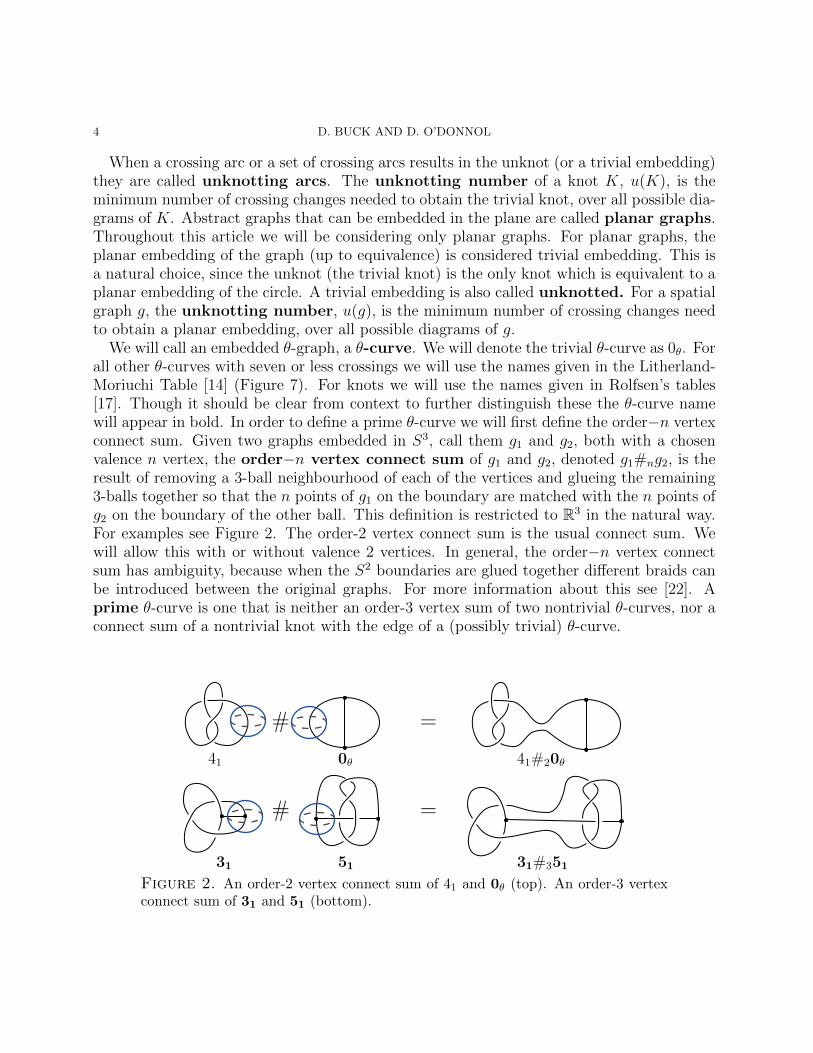
We will call an embedded θ-graph, a θ-curve. We will denote the trivial θ-curve as 0θ. Forall other θ-curves with seven or less crossings we will use the names given in the Litherland-Moriuchi Table [14] (Figure 7). For knots we will use the names given in Rolfsen’s tables[17]. Though it should be clear from context to further distinguish these the θ-curve namewill appear in bold. In order to define a prime θ-curve we will first define the order−n vertexconnect sum. Given two graphs embedded in S3, call them g1 and g2, both with a chosenvalence n vertex, the order−n vertex connect sum of g1 and g2, denoted g1#ng2, is theresult of removing a 3-ball neighbourhood of each of the vertices and glueing the remaining3-balls together so that the n points of g1 on the boundary are matched with the n points ofg2 on the boundary of the other ball. This definition is restricted to R3 in the natural way.For examples see Figure 2. The order-2 vertex connect sum is the usual connect sum. Wewill allow this with or without valence 2 vertices. In general, the order−n vertex connectsum has ambiguity, because when the S2 boundaries are glued together different braids canbe introduced between the original graphs. For more information about this see [22]. Aprime θ-curve is one that is neither an order-3 vertex sum of two nontrivial θ-curves, nor aconnect sum of a nontrivial knot with the edge of a (possibly trivial) θ-curve.

=#

41 0θ 41#20θ

=#

31 51 31#351

Figure 2. An order-2 vertex connect sum of 41 and 0θ (top). An order-3 vertexconnect sum of 31 and 51 (bottom).


3. Observations

In this section, we present two bounds on the unknotting number of a spatial graph.Additionally, we define the maximal constituent unknotting number of g.

Observation 2. The unknotting number of spatial graphs is subadditive. Let g1 and g2 beembedded graphs and let g1#ng2 be the order−n vertex connect sum of them. Then

u(g1#ng2) ≤ u(g1) + u(g2).

The minimum crossing changes needed to unknot both g1 and g2 can be described by setsof unknotting arcs αi and βi, respectively. The order−n connect sum can be done withoutdisturbing the unknotting arcs, because the ball can be isotoped to not meet the unknottingarcs. Then the set αi ∪ βi will be a set of unknotting arcs for g1#ng2. Thus u(g1#ng2) is atmost the sum of u(g1) and u(g2).

When possible we will use known unknotting numbers of knots to determine bounds onthe unknotting numbers for spatial graphs. Two constituents are said to overlap if theyshare one or more edges.

Definition 3. Let g be an embedding of a planar graph G. Let s = {K1, . . . , Kn} be a setof mutually non-overlapping constituents of G. The unknotting number of s is,

u(s) =∑Ki∈s

u(Ki).

The maximal constituent unknotting number of g is

mcu(g) = max{u(s)|s is a non-overlapping set of constituents of g}.

The maximal constituent unknotting number is an invariant of the spatial graph.There is a relationship between the unknotting number of g and the maximal constituent

unknotting number of g.

Observation 4. Let g be an embedding of a planar graph G, then u(g) ≥ mcu(g).

When the graph g is unknotted each of its subgraphs are also unknotted. The constituentknots are special cases of subgraphs. If one of the constituents is not unknotted then thegraph will not be unknotted. Since we are considering non-overlapping constituents, un-knotting one will not affect the others. Thus there must be at least enough crossing changesto unknot the set of non-overlapping constituent knots with the largest sum of unknottingnumbers.

Turning our attention to the θ-graph, all of the constituents of a θ-curve overlap. So themaximal constituent unknotting number reduces to

mcu(θ) = max{u(Ki)|Ki are the full set of constituent knots}.If we instead consider the sum of the unknotting numbers of all of the constituents of aθ-curve we see that this can have any relationship with u(θ). Let Ki be the constituents of


θ for i = 1, 2, 3. We have

u(θ) > u(K1) + u(K2) + u(K3)

for θ = 51 and 61, however

u(θ) = u(K1) + u(K2) + u(K3)

for θ = 31 and 612, and finally

u(θ) < u(K1) + u(K2) + u(K3)

for θ = 57 and 616. There are many more examples in each of these instances. However, theonly prime θ-curves with 7 or less crossing, for which u(θ) > u(K1) + u(K2) + u(K3) holdsare those where all of the constituents are unknots. It would be interesting to find a primeθ-curve for which u(θ) > u(K1) + u(K2) + u(K3) holds that has nontrivial constituents.

4. The unknotting number of prime θ-curves up to 7 crossings

In [14], Moriuchi presented a table of all prime up to 7 crossings, originally compiledby Litherland. Moriuchi showed that all of the 90 θ-curves appearing in the table aredistinct. While the completeness of Litherland’s table has not been proven, the independentconstruction by Moriuchi of the prime θ-curves up to 7 crossings using a variation of Conway’smethods gave the same set of θ-curves. See Figure 7.

We have determined u(g) for all but four of the θ-curves in the Litherland-Moriuchi Table.In Figure 7, we indicate a set of crossing changes that will unknot each θ-curve. We firstdemonstrate unknotting curves, then show they are minimal.

Proposition 5. The crossing changes indicated in Figure 7 unknot each of the curves.

Proof. The unknotting crossing changes are highlighted in gray (purple). One can check thatall of the θ-curves are unknotted with the indicated changes. For example, Figure 3 showshow 57 can be moved to a planar embedding via Reidemeister moves after the indicatedcrossing change. �

II I V V

57 θo

Figure 3. The θ-curve 57 with unknotting crossing change. The arrow indicatesthe highlighted crossing change, and the double arrows are the indicated Reidemeis-ter moves.


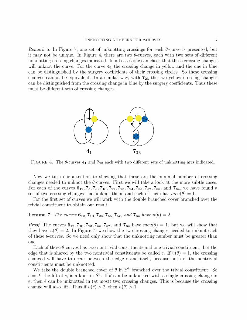
Remark 6. In Figure 7, one set of unknotting crossings for each θ-curve is presented, butit may not be unique. In Figure 4, there are two θ-curves, each with two sets of differentunknotting crossing changes indicated. In all cases one can check that these crossing changeswill unknot the curve. For the curve 41 the crossing change in yellow and the one in bluecan be distinguished by the surgery coefficients of their crossing circles. So these crossingchanges cannot be equivalent. In a similar way, with 723 the two yellow crossing changescan be distinguished from the crossing change in blue by the surgery coefficients. Thus thesemust be different sets of crossing changes.

41 723

Figure 4. The θ-curves 41 and 723 each with two different sets of unknotting arcs indicated.

Now we turn our attention to showing that these are the minimal number of crossingchanges needed to unknot the θ-curves. First we will take a look at the more subtle cases.For each of the curves 612,75,78,710,722,723,724,755,757,758, and 764, we have found aset of two crossing changes that unknot them, and each of them has mcu(θ) = 1.

For the first set of curves we will work with the double branched cover branched over thetrivial constituent to obtain our result.

Lemma 7. The curves 612,710,723,755,757, and 764 have u(θ) = 2.

Proof. The curves 612,710,723,755,757, and 764 have mcu(θ) = 1, but we will show thatthey have u(θ) = 2. In Figure 7, we show the two crossing changes needed to unknot eachof these θ-curves. So we need only show that the unknotting number must be greater thanone.

Each of these θ-curves has two nontrivial constituents and one trivial constituent. Let theedge that is shared by the two nontrivial constituents be called e. If u(θ) = 1, the crossingchanged will have to occur between the edge e and itself, because both of the nontrivialconstituents must be unknotted.

We take the double branched cover of θ in S3 branched over the trivial constituent. Soe = J , the lift of e, is a knot in S3. If θ can be unknotted with a single crossing change ine, then e can be unknotted in (at most) two crossing changes. This is because the crossingchange will also lift. Thus if u(e) > 2, then u(θ) > 1.


In Table 1, for each θ-curve we give the knot e and its unknotting number. The knot typewas identified using KnotSketcher [7] and KnotFinder [5]. Unknotting numbers were deter-mined from KnotInfo [6]. So based on the unknotting number of e, the curves 612,710,723,755,757, and 764 cannot have unknotting number one. �

Table 1. For each θ-curve e = J is the knot that is the lift of the third edgein the double branched cover of θ branched over the unknotted constituent ofθ. The θ-curve 75 has two unknotted constituents. Both lifts give the sameresult. The knot type of J was identified using KnotSketcher and KnotFinder.Unknotting numbers were determined from KnotInfo.

θ e = J u(J)

612 910 3

75 11n38 1

78 946 2

710 12n574 5

722 10144 2

723 12n503 3

Space

θ e = J u(J)

724 10138 2

755 938 3

757 11a186 3

758 11a14 [2, 3]

764 12a518 4

Figure 5. Knot in solid torus.

For the next technique we will need another definition and theorem. A double knot is aknot that results from embedding the solid torus in Figure 5 containing the knot K into S3,as long as it is nontrivial. In work by A. Coward and M. Lackenby they proved:

Theorem 8. [8] If K is a double knot, but K 6= 41 then there is a unique crossing circle (atthe clasp) and for K = 41 there are exactly 2 (at the two clasps).

Lemma 9. The unknotting number u(78) = 2.

Proof. The curve 78 has mcu(θ) = 1 but we will show that u(θ) = 2. In Figure 7, we showthe two crossing changes needed to unknot 78. So we need only show that the unknottingnumber must be greater than one.

The two nontrivial constituents in 78 are both 31. By Theorem 8 there is a unique crossingcircle for each of these constituents. To have u(78) = 1 there must be a way to move the


circles in the exterior of their respective knots so that they indicate the same crossing changein 78. However, these two trefoils are mirror images of each other; so the surgery coefficientsare +1 and −1. See Figure 6. So this is not possible. �

−1

+1

78

+1

−1

710

Figure 6. The θ-curves 78 and 710 with the unique crossing circles with differentsurgery coefficients shown. The common edge of the two nontrivial constituents is

bold.

Note: This method can also be used to prove u(710) = 2.

Theorem 10. The unknotting numbers for the θ-curves in the Litherland-Moriuchi Tableare determined exactly for all but 75, 722, 724, and 758 which have unknotting number 1 or2. See Table 2. Additionally, unknotting crossing changes are shown for all of the curves inFigure 7.

In the Appendix, Theorem 11 shows that the θ–curves 75, 722, 724, and 758 all haveunknotting number 2.

Proof. The θ-curves 51,61,71,72,73, and 74 are all examples of nontrivial θ-curves where allof the constituent knots are unknots. (A list of the θ-curves together with their constituentknots is given in Table 2.) So they must have at least unknotting number 1. These were allshown to have u(θ) = 1 by finding an unknotting crossing. See Figure 7.

For the remaining θ-curves, those with nontrivial constituents, we use Observation 4. Itsays u(θ) ≥ mcu(θ). With the exception of the 11 curves 612,75,78,710,722,723, 724,755,757,758, and 764, the remaining curves had u(θ) = mcu(θ). See Figure 7.

It was shown in Lemma 7 and Lemma 9 that the curves 612,78,710,723, 755,757, and 764

have u(θ) = 2. The four remaining curves 75,722, 724, and 758 have mcu(θ) = 1 howeverthe only known means of unknotting take two crossing changes. So the unknotting numberfor these curves is 1 or 2. This completes our proof. �


Table 2. Theta curves, their constituents, their maximal constituent unknot-ting number, and their unknotting numbers.

θ C. Knots mcu u

31 2x01 31 1 1

41 2x01 41 1 1

51 3x01 0 1

52 2x01 31 1 1

53 2x01 51 2 2

54 01 31 51 2 2

55 2x01 52 1 1

56 2x01 52 1 1

57 01 31 52 1 1

61 3x01 0 1

62 2x01 31 1 1

63 01 31 41 1 1

64 01 31 41 1 1

65 2x01 61 1 1

66 2x01 61 1 1

67 2x01 61 1 1

68 01 41 61 1 1

69 2x01 62 1 1

610 2x01 62 1 1

611 2x01 62 1 1

612 01 31 62 1 2

613 01 41 62 1 1

614 2x01 63 1 1

615 2x01 63 1 1

616 01 31 63 1 1

71 3x01 0 1

72 3x01 0 1

73 3x01 0 1

74 3x01 0 1

75 2x01 31 1 2

θ C. Knots mcu u

76 2x01 31 1 1

77 2x01 31 1 1

78 01 31 31 1 2

79 01 31 31 1 1

710 01 31 31 1 2

711 2x01 52 1 1

712 2x01 41 1 1

713 2x01 41 1 1

714 01 41 41 1 1

715 2x01 51 2 2

716 2x01 51 2 2

717 2x01 51 2 2

718 01 51 52 2 2

719 2x01 52 1 1

720 2x01 52 1 1

721 2x01 52 1 1

722 01 31 52 1 2

723 01 41 52 1 2

724 01 41 52 1 2

725 2x01 71 3 3

726 01 31 71 3 3

727 01 51 71 3 3

728 2x01 72 1 1

729 2x01 72 1 1

730 2x01 72 1 1

731 01 31 72 1 1

732 01 52 72 1 1

733 2x01 73 2 2

734 2x01 73 2 2

735 01 31 73 2 2

θ C. Knots mcu u

736 01 51 73 2 2

737 01 52 73 2 2

738 2x01 74 2 2

739 2x01 74 2 2

740 01 31 74 2 2

741 01 31 74 2 2

742 01 52 74 2 2

743 2x01 75 2 2

744 2x01 75 2 2

745 01 31 75 2 2

746 01 31 75 2 2

747 01 31 75 2 2

748 01 51 75 2 2

749 01 52 75 2 2

750 2x01 76 1 1

751 2x01 76 1 1

752 2x01 76 1 1

753 2x01 76 1 1

754 2x01 76 1 1

755 01 31 76 1 2

756 01 31 76 1 1

757 01 41 76 1 2

758 01 52 76 1 2

759 2x01 77 1 1

760 2x01 77 1 1

761 2x01 77 1 1

762 2x01 77 1 1

763 2x01 77 1 1

764 01 31 77 1 2

765 01 41 77 1 1

Appendix A. On bandings of unknotting number 1 θ–curves

Kenneth l. Baker

In Theorem 10 above, Buck-O’Donnol determine the unknotting numbers for all θ–curvesin the Litherland-Moriuchi table [14] of prime knotted θ–curves that admit diagrams with at


most 7 crossings, except for the θ–curves 75, 722, 724, and 758. In this appendix we provideanother method for showing the unknotting number of a θ–curve is not 1 which allows us toconfirm that the unknotting numbers of each of these four θ–curves is 2.

Theorem 11. The unknotting numbers of the θ–curves 75, 722, 724, and 758 are all 2.

Labeling the three edges of a θ–curve θ as e1, e2, e3, we obtain three constituent knotsKi = θ − Int ei, for i = 1, 2, 3, obtained by deleting the interior of an edge. Buck-O’Donnoldefine the maximal constituent unknotting number of a θ–curve θ with constituentknots K1, K2, and K3 to be

mcu(θ) = max{u(K1), u(K2), u(K3)},and they observe that u(θ) ≥ mcu(θ). See Definition 3 and Observation 4.

Instead of deleting an edge of the θ–curve θ, we may use the edge ei to determine bandingsof the constituent knot Ki to a family of two-component links Lni as follows: Choose anorientation on the edges of θ so that they all begin at the same vertex. For {i, j, k} = {1, 2, 3},band Ki along ei to produce a two component link. (Specifically, for the interval I = [−1, 1],let b be an embedding of the rectangle I × I into S3 so that b({0}× I) = ei, b(I × ∂I) ⊂ Ki,and (Ki−b(I×I))∪b(∂I×I) is a link of two components.) The resulting link has componentsisotopic to the constituent knots Kj and Kk that we orient according to the orientations onthe edges ej and ek. Since any two of these bandings along ei differ by an integral numberof full twists in the band, the resulting links are distinguished by their linking numbers. LetLni be the one whose components have linking number n.

Lemma 12. If u(θ) = 1, then for some i = 1, 2, 3, either

(1) at least one component of L0i is unknotted and u(L0

i ) ≤ 1, or(2) both components of L0

i are unknotted and either u(L1i ) = 1 or u(L−1i ) = 1.

Let us emphasize here that, as a link L of m components may be viewed as a knottedplanar graph, its unknotting number u(L) is the minimum number of crossing changes neededto obtain the m–component unlink.

Proof. Let θ0 be the unknotted θ–curve embedded in the sphere S. If u(θ) = 1, then there isa crossing disk D for θ0 such that ±1–surgery on the crossing circle ∂D produces θ. Observethat D is disjoint from an edge ei of θ0. Banding θ0 along ei with a rectangle in S producesthe two-component unlink in S. Since such a rectangle may be chosen to lie in an arbitrarilysmall neighborhood of ei, it may be taken to be disjoint from D as well. Therefore theoperations of the banding and ±1–surgery on ∂D commute.

Banding along ei after ±1–surgery on ∂D thus produces one of the links Lni . Then per-forming ∓1–surgery on the image of ∂D produces the unlink as this undoes the ±1–surgeryleaving only the banding from θ0. Hence u(Lni ) ≤ 1.

Note that u(Lni ) ≥ u(Kj) + u(Kk) + |n|. (Any crossing change either involves only asingle component and preserves linking number or involves both components to alter thelinking number while preserving the knot types of the components.) If u(Lni ) = 0, then Lniis the unlink and n = 0. If u(Lni ) = 1 and the trivializing crossing change involves only onecomponent of Lni , then n = 0 and the other component must be an unknot. If u(Lni ) = 1


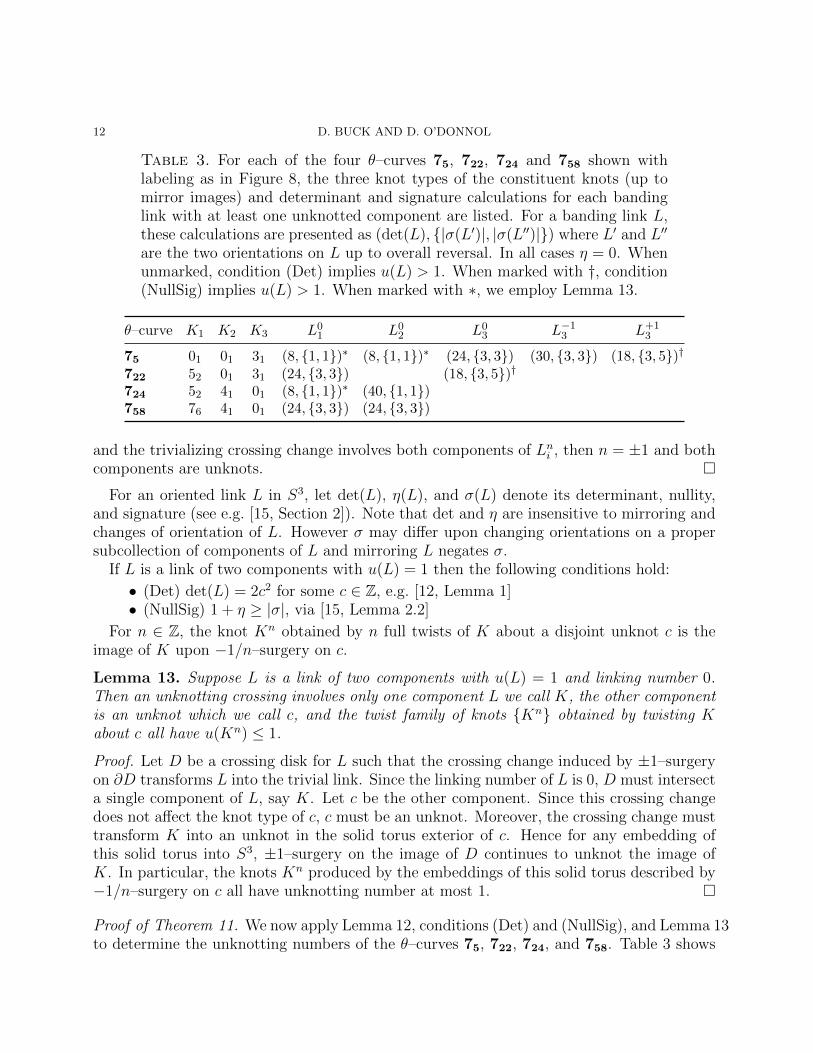
Table 3. For each of the four θ–curves 75, 722, 724 and 758 shown withlabeling as in Figure 8, the three knot types of the constituent knots (up tomirror images) and determinant and signature calculations for each bandinglink with at least one unknotted component are listed. For a banding link L,these calculations are presented as (det(L), {|σ(L′)|, |σ(L′′)|}) where L′ and L′′

are the two orientations on L up to overall reversal. In all cases η = 0. Whenunmarked, condition (Det) implies u(L) > 1. When marked with †, condition(NullSig) implies u(L) > 1. When marked with ∗, we employ Lemma 13.

θ–curve K1 K2 K3 L01 L0

2 L03 L−13 L+1

3

75 01 01 31 (8, {1, 1})∗ (8, {1, 1})∗ (24, {3, 3}) (30, {3, 3}) (18, {3, 5})†722 52 01 31 (24, {3, 3}) (18, {3, 5})†724 52 41 01 (8, {1, 1})∗ (40, {1, 1})758 76 41 01 (24, {3, 3}) (24, {3, 3})

and the trivializing crossing change involves both components of Lni , then n = ±1 and bothcomponents are unknots. �

For an oriented link L in S3, let det(L), η(L), and σ(L) denote its determinant, nullity,and signature (see e.g. [15, Section 2]). Note that det and η are insensitive to mirroring andchanges of orientation of L. However σ may differ upon changing orientations on a propersubcollection of components of L and mirroring L negates σ.

If L is a link of two components with u(L) = 1 then the following conditions hold:

• (Det) det(L) = 2c2 for some c ∈ Z, e.g. [12, Lemma 1]• (NullSig) 1 + η ≥ |σ|, via [15, Lemma 2.2]

For n ∈ Z, the knot Kn obtained by n full twists of K about a disjoint unknot c is theimage of K upon −1/n–surgery on c.

Lemma 13. Suppose L is a link of two components with u(L) = 1 and linking number 0.Then an unknotting crossing involves only one component L we call K, the other componentis an unknot which we call c, and the twist family of knots {Kn} obtained by twisting Kabout c all have u(Kn) ≤ 1.

Proof. Let D be a crossing disk for L such that the crossing change induced by ±1–surgeryon ∂D transforms L into the trivial link. Since the linking number of L is 0, D must intersecta single component of L, say K. Let c be the other component. Since this crossing changedoes not affect the knot type of c, c must be an unknot. Moreover, the crossing change musttransform K into an unknot in the solid torus exterior of c. Hence for any embedding ofthis solid torus into S3, ±1–surgery on the image of D continues to unknot the image ofK. In particular, the knots Kn produced by the embeddings of this solid torus described by−1/n–surgery on c all have unknotting number at most 1. �

Proof of Theorem 11. We now apply Lemma 12, conditions (Det) and (NullSig), and Lemma 13to determine the unknotting numbers of the θ–curves 75, 722, 724, and 758. Table 3 shows


the calculations of determinant and signature (the nullity is always 0) which are sufficientto conclude the relevant banding links have unknotting number greater than 1 in all casesexcept three, the links L0

1 and L02 of 75 and L0

1 of 724. To perform these calculations, weused PLink from within SnapPy [9] to draw the links and obtain their PD code. Then weused a program of Owens [16] built on the KnotTheory‘ package [2] for Mathematica [23] tocompute the determinant, nullity, and signature from the PD codes of these links.

For the links L01 and L0

2 of 75, observe that 75 admits an orientation preserving involu-tion that exchanges edges e1 and e2 and reverses e3. This becomes apparent from a slightredrawing of 75 in which the diagram has 8 crossings and a vertical axis of symmetry. Hencethe links L0

1 and L02 are actually isotopic.

Focusing then on the link L01 of 75, SnapPy informs us that performing −1–surgery on the

unknotted component K2 of L01 produces the knot 11n79 for which u(11n79) = 2 is reported

on KnotInfo [6]. (Knotorious [3] reports that the algebraic unknotting number of 11n79 is2 due to the “Lickorish Test” [12, Lemma 2]. By inspection, one sees that it is at most 2.)Therefore u(L0

1) > 1 by Lemma 13. Hence we also have that u(L02) > 1 for the link L0

2 of 75.

For the link L01 of 724, SnapPy informs us that performing −1–surgery on the unknotted

component K3 of L01 produces the alternating knot 74 for which u(74) = 2 is reported on

KnotInfo [6]. (Here too Knotorious [3] reports that the algebraic unknotting number of theknot 74 is 2 due to the “Lickorish Test” [12, Lemma 2]. By inspection, one sees that it is atmost 2.) Therefore u(L0

1) > 1 by Lemma 13.Taken together, Lemma 12 shows that the θ–curves 75, 722, 724, and 758 all must have

unlinking number 2. �

References

[1] D. E. Adams, E. M. Shekhtman, E. L. Zechiedrich, M. B. Schmid, and N. R. Cozzarelli, The role oftopoisomerase IV in partitioning bacterial replicons and the structure of catenated intermediates in DNAreplication, Cell 71 (1992), no. 2, 277–288.

[2] D. Bar-Natan, S. Morrison, and et al., The Mathematica Package knottheory‘, Available at http:

//katlas.org/wiki/The_Mathematica_Package_KnotTheory (10/2017).[3] M. Borodzik and S. Friedl, Knotorious, https://www.mimuw.edu.pl/ mcboro/knotorious.php.[4] D. Buck, D. O’Donnol and A. Stasiak, Knotting of replication intermediates is tightly prescribed,

Preprint.[5] J. Cha and C. Livingston, Knotfinder from Knotinfo, Available at http://www.indiana.edu/

~knotinfo/knotfinder.html (2017/09/28).[6] , Knotinfo: Table of knot invariants, Available at http://www.indiana.edu/~knotinfo

(2017/10/20).[7] , Knotsketcher from Knotinfo, Available at http://www.indiana.edu/~knotinfo/

knotsketcher.html (2017/09/28).[8] A. Coward and M. Lackenby, Unknotting genus one knots, Comment. Math. Helv. 86 (2011), no. 2,

383–399.[9] M. Culler, N. M. Dunfield, M. Goerner, and J. R. Weeks, SnapPy, a computer program for studying the

geometry and topology of 3-manifolds, Available at http://snappy.computop.org (10/2017).[10] L. H. Kauffman, Invariants of graphs in three-space, Trans. Amer. Math. Soc. 311 (1989), no. 2, 697–710.[11] A. Kawauchi, On transforming a spatial graph into a plane graph, 191 (2011), 225–234.

http://katlas.org/wiki/The_Mathematica_Package_KnotTheory

http://katlas.org/wiki/The_Mathematica_Package_KnotTheory

http://www.indiana.edu/~knotinfo/knotfinder.html

http://www.indiana.edu/~knotinfo/knotfinder.html

http://www.indiana.edu/~knotinfo

http://www.indiana.edu/~knotinfo/knotsketcher.html

http://www.indiana.edu/~knotinfo/knotsketcher.html

http://snappy.computop.org


[12] W. B. R. Lickorish, The unknotting number of a classical knot, Combinatorial methods in topology andalgebraic geometry (Rochester, N.Y., 1982), Contemp. Math., vol. 44, Amer. Math. Soc., Providence,RI, 1985, pp. 117–121.

[13] V. Lopez, M. L. Martinez-Robles, P. Hernandez, D. B. Krimer, and J. B. Schvartzman, Topo IV is thetopoisomerase that knots and unknots sister duplexes during DNA replication, Nucleic Acids Res. 40(2012), no. 8, 3563–3573.

[14] H. Moriuchi, An enumeration of theta-curves with up to seven crossings, J. Knot Theory Ramifications18 (2009), no. 2, 167–197.

[15] M. Nagel and B. Owens, Unlinking information from 4-manifolds, Bull. Lond. Math. Soc. 47 (2015),no. 6, 964–979.

[16] B. Owens, Mathematica programs, Available at http://www.maths.gla.ac.uk/~bowens/ (10/2017).[17] D. Rolfsen, Knots and links, 1990.[18] D. Santamaria, G. de la Cueva, M. L. Martinez-Robles, D. B. Krimer, P. Hernandez, and J. B. Schvartz-

man, DnaB helicase is unable to dissociate RNA-DNA hybrids. Its implication in the polar pausing ofreplication forks at ColE1 origins, J. Biol. Chem. 273 (1998), no. 50, 33386–33396.

[19] M. Scharlemann and A. Thompson, Detecting unknotted graphs in 3-space, J. Differential Geom. 34(1991), no. 2, 539–560.

[20] J. K. Simon and K. Wolcott, Minimally knotted graphs in S3, Topology Appl. 37 (1990), no. 2, 163–180.[21] E. Viguera, P. Hernandez, D. B. Krimer, A. S. Boistov, R. Lurz, J. C. Alonso, and J. B. Schvartzman,

The ColE1 unidirectional origin acts as a polar replication fork pausing site, J. Biol. Chem. 271 (1996),no. 37, 22414–22421.

[22] K. Wolcott, The knotting of theta curves and other graphs in s3, Lecture Notes in Pure and AppliedMathematics, vol. 105, Dekker, New York NY, 1987.

[23] Wolfram Research, Mathematica, Version 11.2, Champaign, IL, 2017.

Department of Mathematics, University of Bath, Claverton Down, Bath, England BA27AY

E-mail address: [email protected]

Department of Mathematics, Indiana University Bloomington, 831 E. Third Street, Bloom-ington, IN 47405

E-mail address: [email protected]

Department of Mathematics, University of Miami, Coral Gables, FL 33146, USAE-mail address: [email protected]

http://www.maths.gla.ac.uk/~bowens/


31 41 51 52 53

54 55 56 57 61

62 63 64 65 66

67 68 69 610 611

612 613 614 615 616

71 72 73 74 75

Figure 7. Theta curves with their unknotting crossing changes shown in gray (purple).


76 77 78 79 710

711 712 713 714 715

716 717 718 719 720

721 722 723 724 725

726 727 728 729 730

731 732 733 734 735

Figure 7. continued. Theta curves with their unknotting crossing changesshown in gray (purple).


736 737 738 739 740

741 742 743 744 745

746 747 748 749 750

751 752 753 754 755

756 757 758 759 760

761 762 763 764 765

Figure 7. continued. Theta curves with their unknotting crossing changesshown in gray (purple).


Figure 8. The four θ–curves 75, 722, 724, and 758 are each shown with alabeling of their edges and their bandings L0

1, L02, and L0

3. For 75 the modifi-cations of L0

3 to produce L+13 and L−13 are also shown.

Documents

AND DANIELLE O’DONNOLyy APPENDIX BY KENNETH L. BAKER …