IN DEGREE PROJECT TECHNOLOGY,FIRST CYCLE, 15 CREDITS

, STOCKHOLM SWEDEN 2018

Analyzing Factors Contributing to the Success of a Team in Dota 2

JOHN ANDERSSON

OSKAR ALIN

KTH ROYAL INSTITUTE OF TECHNOLOGYSCHOOL OF ENGINEERING SCIENCES

www.kth.se

INOM EXAMENSARBETE TEKNIK,GRUNDNIVÅ, 15 HP

, STOCKHOLM SVERIGE 2018

Analys av faktorer som bidrar till ett Dota 2 lags framgång

JOHN ANDERSSON

OSKAR ALIN

KTHSKOLAN FÖR TEKNIKVETENSKAP

www.kth.se

Abstract

Competitive gaming or E-Sport is more popular than ever, this has resulted inan increase in the number of players and tournament prize pools. In traditionalsports demographic factors have been shown to have high predictive power whenit comes to determining a country’s success in the Olympic Games. Similarresults have been found when it comes to E-sport which is why it is interestingto investigate whether there are any differences between regions in Dota 2 aswell. The goal is to analyze factors that contribute to the success of a Dota 2team by building a multiple-regression model. All data is collected from opensources and contains 55 active Dota 2 teams that have been playing between2011 - 2018. The factors in the final model is the sum of the individual playersestimated skill, the skill difference between the highest and lowest rated playerson the team, the number of games the team has played and organization region.The result gives an insight in what a person or organization would want to lookat when researching a team as well as a model that can be used to predict howgood a team will perform.

Sammanfattning

Professionell gaming aven kallat E-Sport (Elektronisk Sport) ar mer populartan nagonsin. Detta har resulterat i allt fler spelare och hogre prispotter itavlingsevenemang. For traditionell sport har demografiska faktorer visat sigvara viktiga nar det kommer till att forutsaga ett lands framgang i de Olymp-iska spelen. Liknande resultat har aven observerats nar det kommer till E-Sportvilket ar varfor det ar intressant att undersoka huruvida det ar nagon skillnadmellan regioner for Dota 2. Malet ar att analysera de faktorer som bidrar tillframgang for ett Dota 2 lag genom en multipel linjar regressionsmodell. Alldata ar insamlad fran publika databaser och innehaller 55 aktiva Dota 2 lagsom har spelat mellan 2011 - 2018. Faktorerna i den slutgiltiga modellen arsumman av spelarnas uppskattade individuella skicklighet, skillnaden i ratingmellan den hogst och lagst rankade spelaren i laget, antalet matcher som lagetspelat och vilken region laget kommer fran. Resultatet ger en uppfattning omvilka faktorer som ar relevanta for en person eller organisation som skulle viljastudera ett lag samt en modell som kan anvandas for att forutsaga hur pass braett lag kan prestera.

Contents

1 Introduction 11.1 Background . . . . . . . . . . . . . . . . . . . . . . . . . . . . . . 11.2 Purpose . . . . . . . . . . . . . . . . . . . . . . . . . . . . . . . . 11.3 Research Question . . . . . . . . . . . . . . . . . . . . . . . . . . 2

2 Theory 32.1 Dota 2 . . . . . . . . . . . . . . . . . . . . . . . . . . . . . . . . . 32.2 Elo . . . . . . . . . . . . . . . . . . . . . . . . . . . . . . . . . . . 52.3 Previous Performance Research . . . . . . . . . . . . . . . . . . . 5

2.3.1 Project Aristotle . . . . . . . . . . . . . . . . . . . . . . . 62.3.2 The Olympic Games . . . . . . . . . . . . . . . . . . . . . 82.3.3 E-Sport . . . . . . . . . . . . . . . . . . . . . . . . . . . . 9

2.4 Multiple Linear Regression . . . . . . . . . . . . . . . . . . . . . 92.4.1 Regression Model . . . . . . . . . . . . . . . . . . . . . . . 92.4.2 Ordinary Least Squares . . . . . . . . . . . . . . . . . . . 102.4.3 Assumptions . . . . . . . . . . . . . . . . . . . . . . . . . 102.4.4 Residuals . . . . . . . . . . . . . . . . . . . . . . . . . . . 11

2.5 Hypothesis Test . . . . . . . . . . . . . . . . . . . . . . . . . . . . 112.5.1 Test for Significance of Regression . . . . . . . . . . . . . 112.5.2 Test on Individual Regression Coefficients . . . . . . . . . 12

2.6 Model Selection . . . . . . . . . . . . . . . . . . . . . . . . . . . . 122.6.1 All Possible Regression . . . . . . . . . . . . . . . . . . . . 122.6.2 Akaike Information Criterion . . . . . . . . . . . . . . . . 132.6.3 Mallow’s Cp . . . . . . . . . . . . . . . . . . . . . . . . . . 13

2.7 Model Errors . . . . . . . . . . . . . . . . . . . . . . . . . . . . . 132.7.1 Heteroscedasticity . . . . . . . . . . . . . . . . . . . . . . 132.7.2 Non-Linearity of Data . . . . . . . . . . . . . . . . . . . . 14

2.8 Model Validation . . . . . . . . . . . . . . . . . . . . . . . . . . . 152.8.1 R2 and R2

Adj . . . . . . . . . . . . . . . . . . . . . . . . . 152.8.2 Cook’s Distance . . . . . . . . . . . . . . . . . . . . . . . 152.8.3 Variance Inflation Factor . . . . . . . . . . . . . . . . . . 162.8.4 Mean Square Error (MSE) . . . . . . . . . . . . . . . . . 162.8.5 Leave-One-Out Cross-Validation . . . . . . . . . . . . . . 17

3 Method 183.1 Demarcation . . . . . . . . . . . . . . . . . . . . . . . . . . . . . 183.2 Variable Selection . . . . . . . . . . . . . . . . . . . . . . . . . . . 18

3.2.1 Response Variable . . . . . . . . . . . . . . . . . . . . . . 183.2.2 Explanatory Variables (Naive Model) . . . . . . . . . . . 183.2.3 Explanatory Variables (Extended Model) . . . . . . . . . 19

3.3 Data Collection . . . . . . . . . . . . . . . . . . . . . . . . . . . . 193.4 Model Selection . . . . . . . . . . . . . . . . . . . . . . . . . . . . 20

4 Results 214.1 Naive Model . . . . . . . . . . . . . . . . . . . . . . . . . . . . . . 21

4.1.1 Validating Naive Initial Model . . . . . . . . . . . . . . . 214.2 Naive Reduced Model . . . . . . . . . . . . . . . . . . . . . . . . 24

4.2.1 Validating Naive Reduced Model . . . . . . . . . . . . . . 244.3 Extended Initial Model . . . . . . . . . . . . . . . . . . . . . . . . 27

4.3.1 Validating Extended Initial Model . . . . . . . . . . . . . 274.4 Extended Reduced Model . . . . . . . . . . . . . . . . . . . . . . 304.5 Validating Extended Reduced Model . . . . . . . . . . . . . . . . 314.6 Model Comparison and Analysis . . . . . . . . . . . . . . . . . . 34

5 Discussion 35

6 Conclusion 37

References 38

A Appendix 40

1 Introduction

1.1 Background

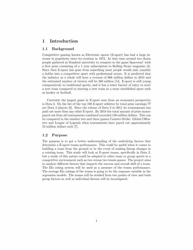
Competitive gaming known as Electronic sports (E-sport) has had a large in-crease in popularity since its creation in 1972. At that time around two dozenpeople gathered at Stanford university to compete in the game Spacewar! witha first prize consisting of a 1 year subscription to Rolling Stone magazine [4].Since then E-sport has gone from something most people would only considera hobby into a competitive sport with professional actors. It is predicted thatthe industry as a whole will have a revenue of 906 million dollars in 2018 andthe estimated number of viewers will be 380 million [14]. E-sport is still youngcomparatively to traditional sports, and it has a lower barrier of entry to starta new team compared to starting a new team in a more established sport suchas hockey or football.

Currently the largest game in E-sport seen from an economics perspectiveis Dota 2. On the list of the top 100 E-sport athletes by total prize earnings 77are Dota 2 players [6]. Since the release of Dota 2 in 2011 its tournaments haspaid out more then any other E-sport. By 2018 the total amount of prize moneypayed out from all tournaments combined exceeded 138 million dollars. This canbe compared to the number two and three games Counter-Strike: Global Offen-sive and League of Legends whos tournaments have payed out approximately52 million dollars each [7].

1.2 Purpose

The purpose is to get a better understanding of the underlying factors thatdetermine a E-sport teams performance. This could be useful when it comes tobuilding a team from the ground or in the event of making lineup changes ina existing team. This study will look at E-sport teams, specifically in Dota 2,but a study of this nature could be adapted to other team or group sports in acompetitive environment such as two versus two tennis games. The project aimsto analyze different factors that impacts the success and overall skill of a team.The Elo rating system will be used as a measure of the teams performance.The average Elo ratings of the teams is going to be the response variable in theregression models. The teams will be studied from two points of view and bothgroup factors as well as individual factors will be investigated.

1

1.3 Research Question

The goal is to create a linear model that can estimate the skill level of a team.Two different models will be tested to find a satisfactory model.

The Naive Model: A model that only includes the individual players es-timated skill and their position in the Dota 2 team.

The Extended Model: A model that includes the combined estimatedskill of all the players but also takes into account the skill difference, the playersnationalities, how many players have represented the team, the region and ageof the team organization and the number of games played.

2

2 Theory

2.1 Dota 2

Dota 2 has a active competitive scene with players from all over the worldcompeting in tournaments and leagues of different sizes. The major Dota 2tournaments have the largest prize pools in all of E-sport and the largest so farwas The International 2017 which had a prize pool of 24,8 million dollars [20].Professional Dota 2 matches are streamed live on websites such as youtube andtwitch.tv and the viewers can reach into the millions.

Dota 2 was released in beta form in 2011 and it is a free to play multiplayeronline battle arena (MOBA) computer game developed by Valve corporation,an American game developer and digital distribution company. It is a sequelto the popular Defense of the Ancients (Dota) which was a community createdmod for Blizzard’s 2002 game Warcraft III [8].

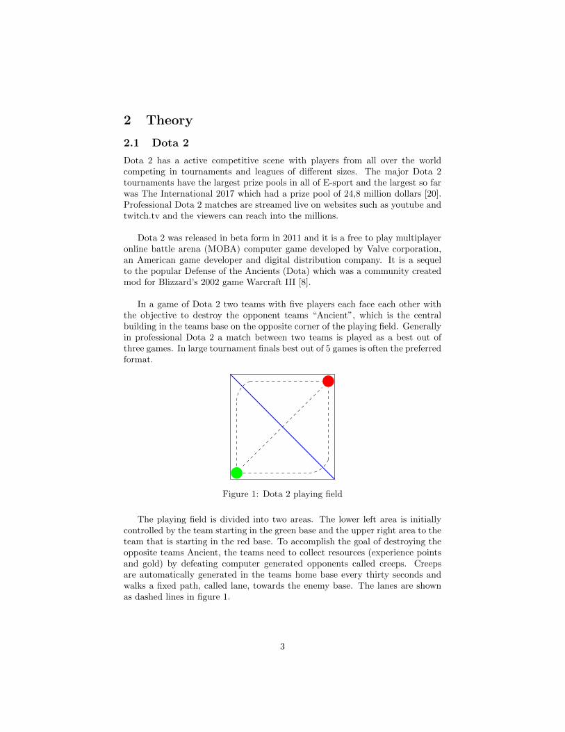
In a game of Dota 2 two teams with five players each face each other withthe objective to destroy the opponent teams “Ancient”, which is the centralbuilding in the teams base on the opposite corner of the playing field. Generallyin professional Dota 2 a match between two teams is played as a best out ofthree games. In large tournament finals best out of 5 games is often the preferredformat.

Figure 1: Dota 2 playing field

The playing field is divided into two areas. The lower left area is initiallycontrolled by the team starting in the green base and the upper right area to theteam that is starting in the red base. To accomplish the goal of destroying theopposite teams Ancient, the teams need to collect resources (experience pointsand gold) by defeating computer generated opponents called creeps. Creepsare automatically generated in the teams home base every thirty seconds andwalks a fixed path, called lane, towards the enemy base. The lanes are shownas dashed lines in figure 1.

3

Each player controls a character that is referred to as a hero. As of 2018-04-12 there are 115 different heroes in the game all with unique abilities and playstyles. Each hero starts at level 1 and has a maximum level of 25. Experiencepoints allows them to level up and increase the power of the heroes abilitiesand gold is used to purchase items that increase the strength the hero. Theheroes can be divided into two primary categories: core heroes and supportheroes. Core heroes main purpose is to inflict as much damage as possible tothe opposite team players and their structures. Core heroes generally start weakbut scale up as they gather more gold and experience. Support heroes focus onassisting the core hero to increase in strength and to gather intelligence aboutthe opposite team, for example monitor enemy movement on the map. Supportheroes often does not need much gold or experience to be useful.

Just like many other team oriented sports Dota 2 players have differentpositions available to them. In soccer the players have different positions suchas goalkeeper, forward and midfielder. In Dota 2 the positions are often referredto by a number which indicated that positions farm priority. Position 1-3 areoften refereed to as core positions while 4 and 5 are the support heroes. Dota 2doesn’t have any fixed positions and can be played many different ways, but acommon lineup is detailed below:

1. Hard Carry: The hard carry is often focused on gaining resources, resultingin a hero that can inflict large amounts of damage as the game goes on.This position is often supported by the number 4 and 5 players early toensure a strong late game.

2. Solo Mid-laner: The solo mid-laner is also focused on gaining gold andexperience, but usually not to the extent of the hard carry. The mid-lanerlevels up faster than the hard carry (because the mid laner is alone andnot sharing the lanes resources with the support) and is usually the maindamage dealer until the hard carry is ready.

3. Solo Offlaner: The offlaners role early is to harass the enemy team’s hardcarry and try to get as much resources as possible.

4. Roamer/Jungler/Secondary-Support: This position is flexible but usuallyit revolves around roaming the map and helping out whichever lane needsassistance.

5. Hard Support: Early in the game the main goal of the hard support is tohelp out the team’s hard carry. The support is also the one that providesvision of the map to his team buy purchasing and placing an in game itemcalled wards.

4

2.2 Elo

The Elo rating system, named after its creator Arpad Elo, is a framework forcomparing the relative skill between different players in zero-sum games. It wasoriginally developed in order to rank chess players but it has since been imple-mented as a rating system for numerous other sports and games. In this systema player will be assigned a numerical rating based on his or her performanceagainst other players. Winning matches increases a players rating and lossesleads to a reduction in rating. In a match where one player has a higher ratingthan his opponent the rating system predicts that higher rated player is morelikely to win. The larger this rating difference is the more favored the higherranked player is in the matchup. This rating difference also dictates how manypoints the winner takes from the loser. If the difference is large and the higherrated player wins he will not gain many of his opponents points, but in the caseof an upset the lower ranked player can gain many of his opponents points.

A central assumption in this model is that every players performance canbe described as a normally distributed random variable whose mean representsthat player’s true skill. For simplification reasons all players are assumed tohave the same standard deviation for their performance random variable [9].

When analyzing paired comparison data, it makes little difference whetherone assumes the logistic distribution or the normal distribution [18]. For thisreason the logistic distribution is most often used when comparing the skill oftwo players since it is simpler. Using this logistic distribution and two playerswith rating RPlayer1 and RPlayer2 respectively the following expressions showstheir expected score:

Eplayer1 =1

1 + 10(RPlayer2−RPlayer1)/400(1)

Eplayer2 =1

1 + 10(RPlayer1−RPlayer2)/400(2)

After a game has been played the players rating can be updated, in the case ofPlayer1 the following formula shows the change in rating:

R∗Player1 = RPlayer1 +K(SPlayer1 − EPlayer1) (3)

Where R∗Player1 is the new rating for Player1, SPlayer1 is the score of the playerachieved in the previous game and K is the K-factor, a factor that determinesthe maximum possible adjustment in rating per game. This factor is often setat K = 16 for masters and K = 32 for newer players.

2.3 Previous Performance Research

Group performance and the factors that contribute to the success of a team is anarea of research where many studies have been done. It is not only relevant whenit comes to a group of athletes, businesses are often segmented and employees

5

work in smaller groups, students have study groups and researchers work inteams in order to make important findings. This section will look at the resultsfrom previous studies.

2.3.1 Project Aristotle

In 2012 Google preformed a large study called Project Aristotle in order tolearn what factors contribute to the success of a team. They were hoping toidentify a perfect mix of individual traits and skills necessary to allow a team toperform at a high level. Over two years they conducted over 200 interviews withtheir employees and examined more than 250 attributes in more than 180 activeGoogle teams. To their surprise they found that who is on the team matters lessthen how the team members interact with each other, how they structure theirwork and view their contributions. They managed to identify five key dynamicsthat set the successful teams apart from other teams at Google. The researchersalso found that individual performance of team members were not significantlyconnected with team effectiveness. The important dynamics or factors are asfollows in order of importance:

1. Psychological safety: Can we take risks on this team without feeling inse-cure or embarrassed?

2. Dependability: Can we count on each other to do high quality work ontime?

3. Structure and clarity: Are goals, roles, and execution plans on our teamclear?

4. Meaning of work: Are we working on something that is personally impor-tant for each of us?

5. Impact of work: Do we fundamentally believe that the work we’re doingmatters?

Psychological Safety Psychological safety is a part of team culture or cor-porate culture where the individual members of the group feel like they cantake risks and speak their mind without being seen as ignorant, incompetent,negative, or disruptive. In a team that has a high level of psychological safety,teammates feel safe to take risks around their team members. They feel confi-dent that no one on the team will embarrass or punish anyone else for admittinga mistake, asking a question, or offering a new idea [10].

This aspect of corporate culture can have large affects on the performance ofa team. A study of the February 1, 2003 Columbia space shuttle disaster foundthat Engineers had noticed that the shuttle was damaged during routine reviewsof videos taken at the launch. However the camera angle was not the best toasses the damage and managers downplayed the threat, noting that foam strikes

6

had caused damage to shuttles in the past but had never resulted in a majoraccident. Some concerned engineers described the foam strike as “the largestever” and asked that additional satellite images of the strike area be taken, buttop managers rejected these requests. Many individuals at NASA reported thatthe group dynamics did not encourage a candid discussion of threats. Meet-ing transcripts revealed that managers did not actively seek dissenting views.Packed agendas inhibited thoughtful discussions of potential threats. Hierarchyand status differences made it difficult for lower level engineers to express theirconcerns [3].

Dependability Several of the advantages that derive from the use of orga-nized or collective production, as opposed to individual, stem from the processof the division of labor and task specialization. Task specialization or the divi-sion of the production process into separate operations allows the human andphysical resources used at each stage of the production process to become moreskilled, specialized, and therefore more productive [11]. Task visibility refers tohow well a task allows for the monitoring and evaluation of individual perfor-mances. When an individual work alone their output can often be measuredeasily and their task visibility is therefore high. In the case of a group workingtogether on obscure task in for example a research and development laboratorythe individuals contribution can be hard to measure and the task visibility istherefor low [11]. This can result in a situation where it is hard to see theindividual workers marginal utility. The employees will have less incentives towork hard and no incentive to improve performance unless conditions allow em-ployees to demonstrate their contributions and to obtain the rewards gainedfrom increased performance [11]. For many productive activities, task special-ization and joint specialization (when a group of two or more individuals worktogether) makes it impractical or too costly to monitor an individual’s perfor-mance or marginal productivity. This means that even though the division oflabor is efficient on technical grounds, it can produce problems of control andcoordination at the social system level [11]. The problem is that the same factorthat increases the potential total output in team or collective production servesto decrease the average outputs of the individual team members. In essence,individuals lack the incentive to increase their performance when their perfor-mance cannot be measured or when rewards are not distributed on the basis oftheir marginal productivity [11].

Structure, Clarity and the Meaning and Impact of Work These as-pects are all about making the workers feel fulfilled and help them see the largerpicture and how their work relates to that. Structure and clarity are about theindividuals understanding of the job expectation and the process of fulfillingthese expectations. It is also about setting specific and attainable goals. Mean-ing helps the workers find a sense of purpose in either the work or the outputand it can be an important tool in increasing the teams effectiveness. Themeaning of the work can be personal and unique for all the individual workers,

7

the meaning can come from many different aspects from financial security orhelping the team succeed. The impact refers to the workers own subjective viewthat their work is important and is making a difference for the team as a whole.Seeing that one’s work is contributing to the success of the organization’s goalscan help reveal impact and keep the workers motivated [10].

Purpose and meaning can be very important tools to motivate a group ofemployees. There is an anecdote about when U.S President John F. Kennedyvisited NASA headquarters for the first time in 1961. Supposedly when hetoured the headquarters he he meet a janitor and asked him what he did. Thejanitor allegedly replied “I’m helping put a man on the moon!”. The story me-diates the idea that a workforce motivated by a strong sense of higher purposeis essential to engagement [16].

The audit, tax, and advisory firm KPMG has focused a lot on enhancing theiremployees sense of purpose. To do this they encouraged everyone at the firm,from the Chairman all they way to the interns, to share their own stories abouthow their work is making a difference. They tried to reframe their roles withinthe firm and encouraged their employees to change their view of themselves.Instead of identifying themselves as professionals executing audit they wantedthem to feel like members of a profession that helps millions of American familiesmake better and informed decisions about investing their life savings. Theywanted to get people talking about purpose to create a narrative that couldconnect their employees with the firm’s history of purposeful work and easiersee their part of the bigger picture. To do so, they began collecting employeestories, highlighting the impactful work already being done, and teaching leadershow to talk about purpose with their people. To achieve their goals they startedwhat they called the 10,000 Stories Challenge, asking their employees to sharestories about the difference they make. They were hoping to get 10,000 storiesbut at the end of the challenge they had received approximately 42,000 stories.Surveys KPMG performed after this challenge showed a strong relationshipbetween leaders who talk about the positive societal impact of their teams’ workand a variety of positive human resources and business indicators. Among theemployees who said that their leaders discuss higher purpose, 94 % said KPMGis a great place to work, But among those employees whose leaders didn’t discusspurpose, the corresponding results was only 66 %. This group also reported theyare three times more likely to think about looking for another job than thosewhose leaders did talk about purpose. Since then KPMG has incorporatedpurpose storytelling training into their leadership development programs [16].

2.3.2 The Olympic Games

In the world of sport team performance is also a subject of much research. TheOlympics is a particularly researched subject since the nature of the event in-volves many different disciplines and athletes from all over the word. Manystudies have been performed with the goal of trying to determine Olympic suc-

8

cess on a country level. One finding is that a nation’s GDP and population arekey factors that can explain why countries perform the way they do at a givenOlympics [1] [2] [5] [17]. This is not a surprising find since a larger populationshould lead to more Olympic caliber athletes available in the nation. A a largeGDP can indicate that that the country has the available resources to supporttheir athletes in the form of coaching, infrastructure and adequate training facil-ities. Additional factors such as host country advantage and the sport traditionsin a country has also been shown as relevant to predict results [17]. Differencesbetween Summer and Winter Olympics have been found. The effect of GDP islarger in the case of Winter Olympics while the effect of population is lower.The host country advantage has also been shown to be smaller in the WinterOlympics [1].

2.3.3 E-Sport

E-Sport is a new area that has not been the subject of much research. Howeverone paper from 2016 aimed to examine whether similar country affects like thosethat was found in the Olympic can be found in E-Sport. Interestingly enoughthe findings showed that the factors GDP and population, the factors mostimportant to predict Olympic success, was not significant when it came to E-Sport. Instead regional performance differences was attributed to other nationalfactors such as high quality education and health care, long term orientationand masculine culture [15].

2.4 Multiple Linear Regression

A regression model is a model built from analyzing the relationship between thevariables in a data set. A multiple regression model is a model that includesmore than one factor, or covariate. All formulas and definitions are from [23]and [19].

2.4.1 Regression Model

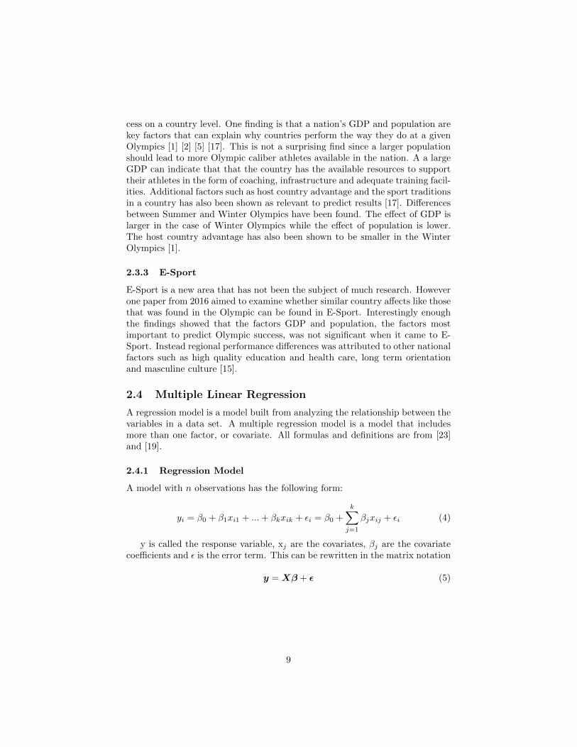
A model with n observations has the following form:

yi = β0 + β1xi1 + ...+ βkxik + εi = β0 +

k∑j=1

βjxij + εi (4)

y is called the response variable, xj are the covariates, βj are the covariatecoefficients and ε is the error term. This can be rewritten in the matrix notation

y = Xβ + ε (5)

9

where the different matrices are

y =

y1y2...yn

X =

1 x11 x12 . . . x1k1 x21 x22 . . . x2k...

......

1 xn1 xn2 . . . xnk

β =

β1β2...βk

ε =

ε1ε2...εn

(6)

The covariate coefficients, βi, are unknown.

2.4.2 Ordinary Least Squares

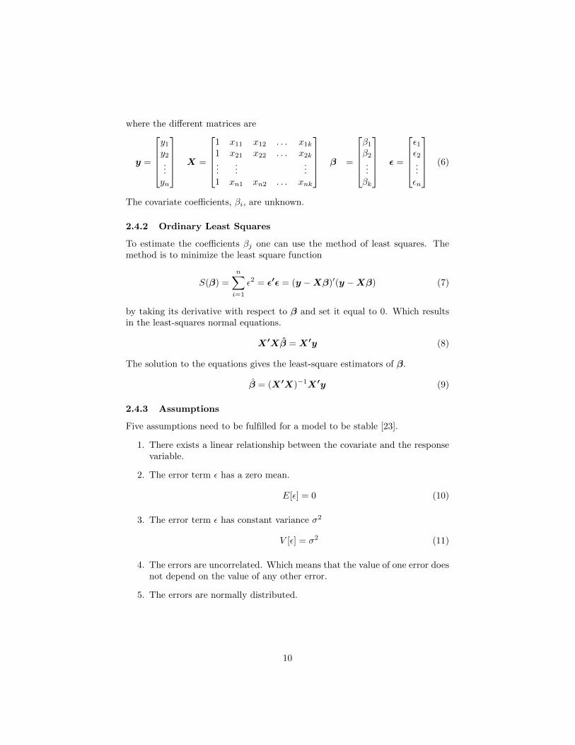
To estimate the coefficients βj one can use the method of least squares. Themethod is to minimize the least square function

S(β) =

n∑i=1

ε2 = ε′ε = (y −Xβ)′(y −Xβ) (7)

by taking its derivative with respect to β and set it equal to 0. Which resultsin the least-squares normal equations.

X′Xβ = X′y (8)

The solution to the equations gives the least-square estimators of β.

β = (X′X)−1X′y (9)

2.4.3 Assumptions

Five assumptions need to be fulfilled for a model to be stable [23].

1. There exists a linear relationship between the covariate and the responsevariable.

2. The error term ε has a zero mean.

E[ε] = 0 (10)

3. The error term ε has constant variance σ2

V [ε] = σ2 (11)

4. The errors are uncorrelated. Which means that the value of one error doesnot depend on the value of any other error.

5. The errors are normally distributed.

10

2.4.4 Residuals

A residual is defined as the difference between the observed value and the fittedvalue

ei = yi − yi, i = 1, 2, ..., n (12)

The residual can be viewed as a measure of the variability of the responsevariable that the fitted model can not explain. It is then convenient to think ofthe residual as the model errors. Meaning that the assumptions for errors mustalso hold for the residuals [23].

2.5 Hypothesis Test

A hypothesis is a educated guess or a proposed explanation to a phenomena. Hy-pothesis testing is used to conclude if the hypothesis proposed from the knowndata is a result by chance or not. One common hypothesis is if there existsa relationship between two variables [19]. To determine if there exists a rela-tionship the two hypothesis are made, the null hypothesis and the alternativehypothesis.

H0 : There is no relationship

H1 : There exists a relationship(13)

2.5.1 Test for Significance of Regression

To determine if there exists a linear relationship between the response variableand the covariates the test for significance of regression can be used [23]. Thetwo hypothesis that are appropriate are

H0 : β1 = β2 = ... = βk = 0

H1 : βj 6= 0 for at least one j(14)

If the null hypothesis is rejected it means that at least one of the covariatescontributes significantly to the model. To test if the relationship exists theF-test can be used. The definition of an F statistic is

F0 =(SST − SSRes)/p

SSRes/(n− p− 1)(15)

p is the number of covariates and n is the number of observations. SSR is thesum of squares due to regression and is defined as

SST = y′y −

( n∑i=1

yi

)2n

(16)

11

and SSRes is the sum of residual squares, defined as

SSRes = y′y − β′X′y (17)

The F statistic follows the Fk,n−k−1 distribution. If F0 > Fα,k,n−k−1, whereα is the level of significance, the null hypothesis is rejected.

2.5.2 Test on Individual Regression Coefficients

When it is determined that there exists a relationship between at least one of thecovariates and the response variable it is interesting to know which covariatesthat is contributing. Adding covariates that does not seem to contribute maylead to a decrease in usefulness for the model. The hypotheses for this test are

H0 : βj = 0

H1 : βj 6= 0(18)

If the null hypothesis is not rejected the covariate xj can be deleted fromthe model. The test statistic for this hypothesis is

to =Bj√σ2Cjj

where σ2 =SSRes

n− 2(19)

Cjj is the diagonal element of the matrix (X′X)−1 corresponding to βj . Toreject the null hypothesis the inequality |t0| > tα/2,n−k−1 must be satisfied.

2.6 Model Selection

2.6.1 All Possible Regression

All possible regression is a method where all possible models are comparedagainst each other [23]. In general with n different covariates there are 2n

models. Since the number of models is exponentially related to the number ofexplanatory variables this method is only suitable when the number of covariatesis relatively low. Lets assume a model with 3 covariates that are denoted x1,x2, x3. Then there is a total of 23 = 8 possible models. Let yn denote the thedifferent models for 1 ≤ n ≤ 8. The models can then be written in the followingway:

y1 = β0 + ε

y2 = β0 + β1x1 + ε

y3 = β0 + β2x2 + ε

y4 = β0 + β3x3 + ε

y5 = β0 + β1x1 + β2x2 + ε

y6 = β0 + β1x1 + β3x3 + ε

y7 = β0 + β2x2 + β3x3 + ε

y8 = β0 + β1x1 + β2x2 + β3x3 + ε

(20)

12

2.6.2 Akaike Information Criterion

The Akaike information criterion (AIC) is a model selection method for com-paring different models against each other. AIC is used to determine whetheror not a covariate should be included in the model. For ordinary least squareregression the AIC is defined as

AIC = nln(SSRes

n

)+ 2p (21)

Where n is the number of observations and p is the number of covariates.To compare models look at:

∆AIC = AICFULL −AICREDUCED (22)

If ∆AIC > 0 the reduced model results in less information loss and is thereforpreferred [13].

2.6.3 Mallow’s Cp

Mallow’s Cp is another model selection method used to assess the fit of a regres-sion model. Mallow’s Cp has been shown to be equivalent to Akaike informationcriterion in the case of Gaussian linear regression. It is defined as

Cp =SSRes(p)

σ2− n+ 2p (23)

n is the number of observations and p is the number of covariates. SSRes(p) isthe residual sum of squares for a p-term subset model [23].

2.7 Model Errors

2.7.1 Heteroscedasticity

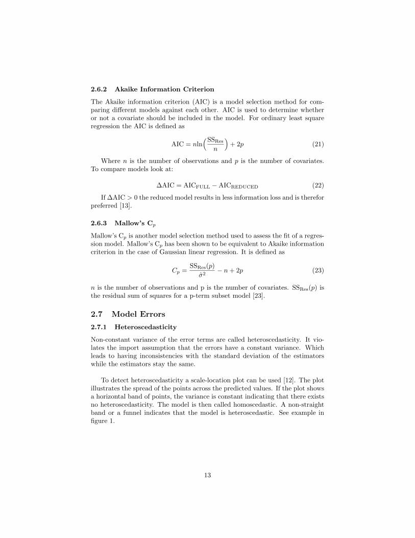
Non-constant variance of the error terms are called heteroscedasticity. It vio-lates the import assumption that the errors have a constant variance. Whichleads to having inconsistencies with the standard deviation of the estimatorswhile the estimators stay the same.

To detect heteroscedasticity a scale-location plot can be used [12]. The plotillustrates the spread of the points across the predicted values. If the plot showsa horizontal band of points, the variance is constant indicating that there existsno heteroscedasticity. The model is then called homoscedastic. A non-straightband or a funnel indicates that the model is heteroscedastic. See example infigure 1.

13

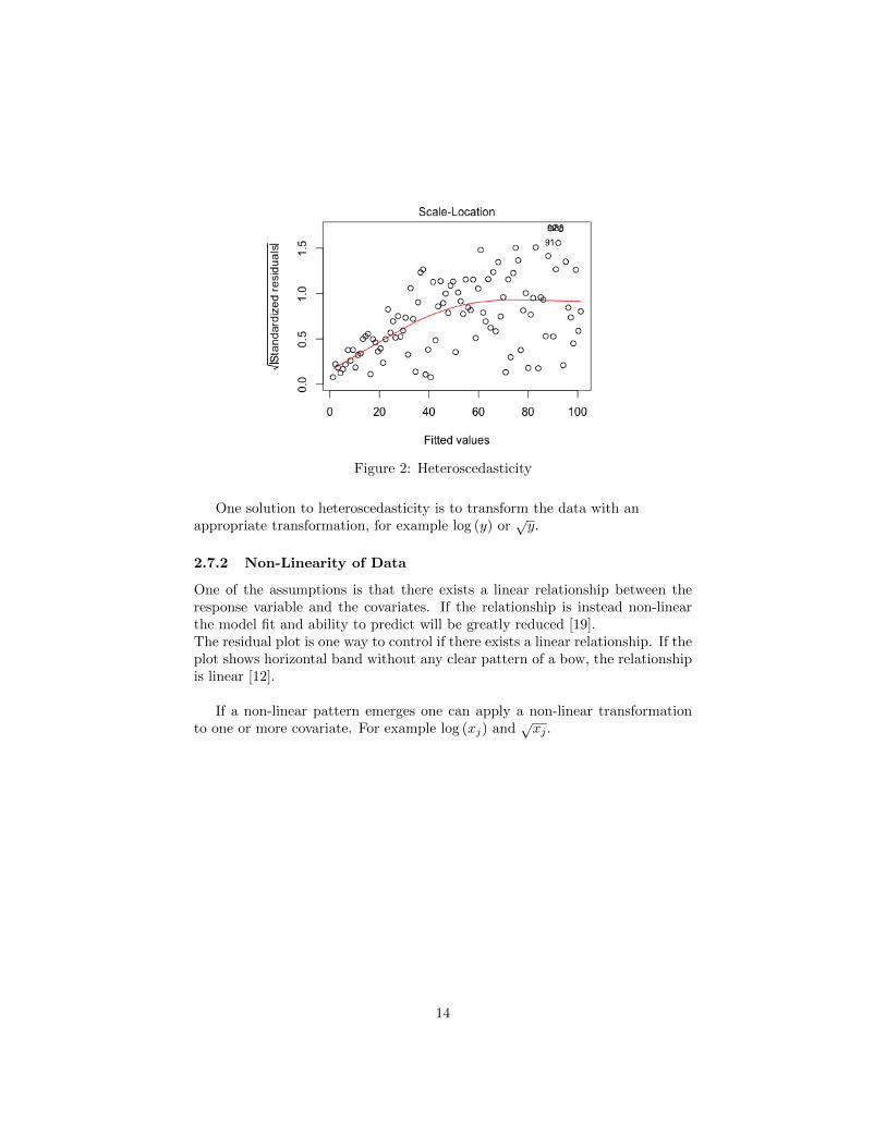
Figure 2: Heteroscedasticity

One solution to heteroscedasticity is to transform the data with anappropriate transformation, for example log (y) or

√y.

2.7.2 Non-Linearity of Data

One of the assumptions is that there exists a linear relationship between theresponse variable and the covariates. If the relationship is instead non-linearthe model fit and ability to predict will be greatly reduced [19].The residual plot is one way to control if there exists a linear relationship. If theplot shows horizontal band without any clear pattern of a bow, the relationshipis linear [12].

If a non-linear pattern emerges one can apply a non-linear transformationto one or more covariate. For example log (xj) and

√xj .

14

Figure 3: Non-linear relationship

2.8 Model Validation

2.8.1 R2 and R2Adj

A tool for comparing different models against each other is the coefficient ofdetermination. Coefficient of determination, or R2, is a statistic that tells theproportion of variance explained by the regressors [19]. It is defined as

R2 = 1− SSRes

SST(24)

Since 0 ≤ SSRes ≤ SST, the value of R2 is between 0 and 1. For example,R2 = 0.89 means that 89% of the variance is explained by the evaluated model.Adding a covariate will increase R2, resulting in an increase even if the covariatedoes not add any value to the model. This could lead to adding terms that areunnecessary for the model. To work around this the R2

Adj statistic will show ifthe additional covariate will improve the model.

R2Adj = 1− SSRes/(n− p− 1)

SST/(n− 1)(25)

2.8.2 Cook’s Distance

Cook’s distance is a measurement commonly used when estimating the influenceof individual data points when performing a regression analysis. It is used tofind data points with a large influence on the overall model which can then bechecked for validity. These data points, outliers and light leverage points candistort the regression model and its accuracy. It works by comparing the least

15

square estimate β based on all data and the estimate βi where observation ihas been deleted. Cook’s distance, denoted Di, of observation i is defined asthe sum of all the changes in the regression model when the observation i isremoved from the dataset. If the model have p covariates the Cook’s distancefor observation i would be given by:

Di =(yi − y)′(yi − y)

pMSReswhere MSRes =

SSRes

n− p(26)

Where y(i) is the response value obtained when excluding observation i.

2.8.3 Variance Inflation Factor

A tool to identify multicollinearity in a model is the variance inflation factors(VIF). It can be written as

VIF =1

1−R2j

(27)

R2j is the coefficient of determination from the linear equation

x1 = α0 + α2x2 + ...+ αkxk (28)

If xj is nearly linearly dependent for some other covariates R2j will approach

1 and VIF will increase. If the value of VIF is larger than 10 there existsmulticollinearity [23].

2.8.4 Mean Square Error (MSE)

The mean squared error (MSE) can be used to measure the quality of a regres-sion method [19]. It is defined as the the average of squared errors

MSE =1

n

n∑i=1

(yi − yi)2 (29)

The value is always a non-negative number. If the MSE is close to zero thefitted values, yi, is close to the observed values.

16

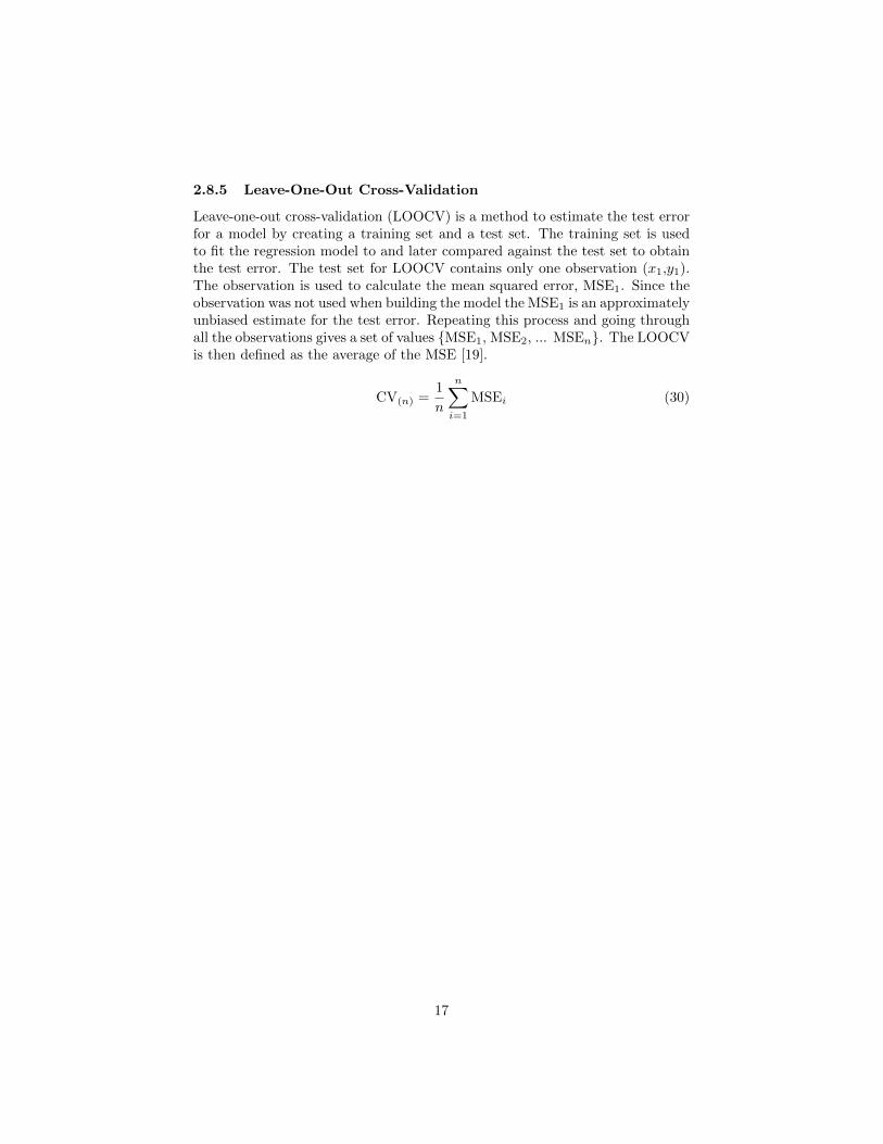
2.8.5 Leave-One-Out Cross-Validation

Leave-one-out cross-validation (LOOCV) is a method to estimate the test errorfor a model by creating a training set and a test set. The training set is usedto fit the regression model to and later compared against the test set to obtainthe test error. The test set for LOOCV contains only one observation (x1,y1).The observation is used to calculate the mean squared error, MSE1. Since theobservation was not used when building the model the MSE1 is an approximatelyunbiased estimate for the test error. Repeating this process and going throughall the observations gives a set of values {MSE1, MSE2, ... MSEn}. The LOOCVis then defined as the average of the MSE [19].

CV(n) =1

n

n∑i=1

MSEi (30)

17

3 Method

3.1 Demarcation

This study is primarily analyzing human factors for high level performance in aDota 2 professional team. The data was collected from open sources due to lim-ited resources. No team, organization or player was contacted for the purposeof collecting data. For example as how much a team trains together, how mucha player plays in their spare time, if the players feel secure with their teammatesand dare to make mistakes, their salaries and more. All these factors could besignificant but are outside the scope of this report. The study only includesactive professional teams that have a Elo rating. To count as a player for theteam, the player needs to have played at least three games (one match) withthe team in a competition.

A time series analysis approach was considered for this project, howeverfinding historical data for the players and teams proved hard. Therefor a crosssectional regression model was chosen instead.

3.2 Variable Selection

The variables were deliberately chosen to reflect the human players and teamcompositions instead of playing styles, hero selection and strategies. The reasonbehind this decision was that the model should reflect the human and not in-game mechanics, even if both surely play a role in how successful a team is.

3.2.1 Response Variable

Average Elo rating The Elo rating changes slightly between every matchplayed between professional teams. The average Elo rating for 30 dayswas chosen to get a value that is relatively stable over a longer period oftime, with K = 32.

3.2.2 Explanatory Variables (Naive Model)

Estimated mmr: The naive model includes five covariates, each being theestimated mmr for a player in the team. Matchmaking rating (mmr) isa numerical value that estimates the skill level for a player [22]. Dota2 measures two different mmr values. Solo mmr and party mmr. Solomeaning playing alone with four unknown players. Party meaning thatyou play together with one or up to four friends in a group. The mmrused in this model is an estimation of the solo mmr.

18

3.2.3 Explanatory Variables (Extended Model)

Total matchmaking rating: All team members combined estimated solo mmr.

Matchmaking rating difference: Taking the difference between the highestand lowest rated player in the team gives the range of how skilled theindividual players on the team are.

Number of games: Total amount of games that the team has played, withany team composition. It might be a indicator how experienced the orga-nization is in a competing environment.

Age of the Dota 2 team: The age of the organizations Dota 2 commitment.The team has not necessarily been active all through out the whole timespan but the organization as such have experience of running a Dota 2team.

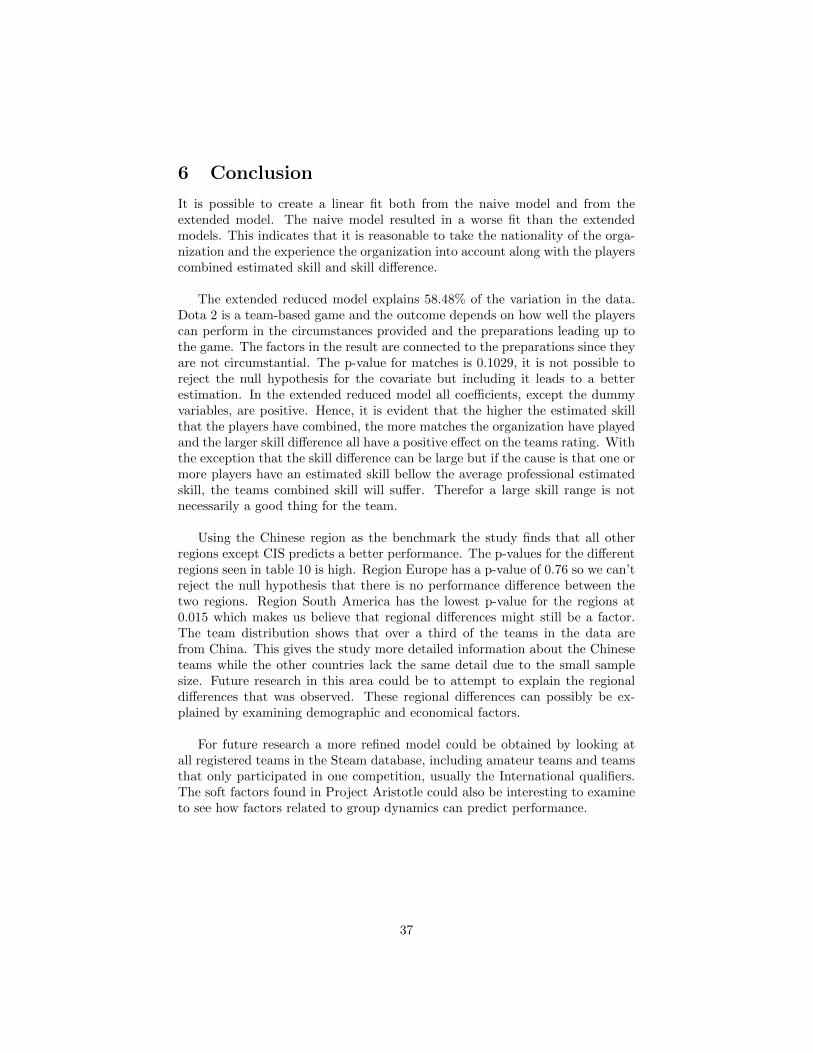
Region of the organization: The Dota 2 community is divided into differ-ent regions. These regions are taken into consideration for example whenteams gets invited to major tournaments, to make sure all regions are rep-resented [21]. These regions are North America, South America, Europe,Commonwealth of Independent States (CIS), China and Southeast Asia.See appendix for region distribution.

Number of different nationalities: How many different nationalities thatare represented in a team. The reason for including this is because dur-ing all team sport some kind of communication takes place and Dota 2.Different nationalities would mean that this communication will probablyrequire the players to talk in a second language.

Total number of players: The sum of total people that have played in theteam, either as a stand-in or as a team player.

3.3 Data Collection

The data was collected from two websites that are using the Steam WebAPI,which gives them direct access to the Steam data base. The average Elo ratingwas downloaded as an excel file from www.datdota.com and the organizationage was manually collected from the same website when going through eachteam in the excel file.

The excel file contained all the teams unique team ID number. A Pythonprogram was written to iterate over the team IDs and to use the ID to downloadjson files by using opendotas own API. All the data was not contained in a sin-gle file so the program needed to download a new file for each team and player.First the total matches was calculated by summing the amount of matches theteams had won and lost. The program proceeded to download the files contain-ing information about how many players the team had been associated with and

19

how many were active. Using the limitation that a player must have to played atleast three games, the program counted how many players that had representedthe team. If there was exactly five active team members, which is the requiredamount to play a game of Dota 2, the program stored their personal player IDand proceeded with downloading the files containing the information about theplayers. From these files the estimated mmr was extracted. The program calcu-lated the total mmr in the team by summing each players estimated mmr. Therange of the mmr was calculated by taking the difference between the largestmmr value and the lowest mmr value. All the data was saved in the same excelfile as earlier.

Nationality of the players and the organizations was manually collectedthrough the websites www.gosugamers.net and www.liquidpedia.net due to lackof options. The data of nationality does not seem to be stored in the Steamdata base or is at least not public.

3.4 Model Selection

An initial model was first fitted using all covariates from the data set. To verifyif the model met the assumptions necessary a residual analysis was conducted,using the diagnostic plots: The Q-Q plot, Residual plot and Scale-location plot.The VIF was calculated for the initial model to make sure that there did notexist any multicollinearity between the covariates, using 10 as the cut off value.Cooks distance was calculated to diagnose if there existed any influential pointsthat could have an unnecessarily high impact on the model. R2, R2

Adj and thecross validation value CV(n) was calculated to be compared with the reducedmodel.

With ”All possible regression” all regression models was generated and tried,using AIC and Cp to compare the different models with each other. A reducedmodel was chosen on the basis of having the lowest AIC and Cp values, comparedto the other models. The same residual analysis was performed to verify that thereduced model met the assumptions needed. R2, R2

Adj and CV(n) was calculatedso it could be compared with the initial model, to see if the model had improvedor not. The process was performed both for the naive model and the extendedmodel. Since the number of models was relatively low, 128 for the extendedmodel, every model was fitted and tried with LOOCV to compare those resultsas well.

20

4 Results

4.1 Naive Model

To decrease the variance a linear transformation with the natural logarithm wasused on the response variable.

log(y) = β0 +

5∑j=1

βjxj (31)

Table 1: Covariates, naive initial model

Datax1 Estimated mmr, position 1x2 Estimated mmr, position 2x3 Estimated mmr, position 3x4 Estimated mmr, position 4x5 Estimated mmr, position 5

4.1.1 Validating Naive Initial Model

The model needs to fulfill the assumptions presented in section 2.4.3. First as-sumption is that there exists a linear relationship between the covariates and theresponse variable. The null hypothesis is that there exists no linear relationshipbetween the response variable and at least one covariate. Using equation (15),F0 is calculated and compared to F0.05,5,49.

7.269 > 2.404 (32)

indicating that at least one βj 6= 0. The p-value is 3.684·10−5, concluding thatthere exists a relationship between the response variable and the covariates.

To further verify this the residuals are plotted against the fitted values.

21

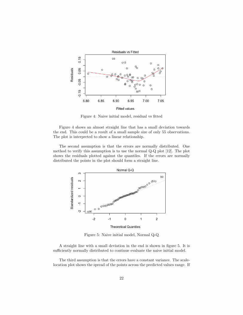
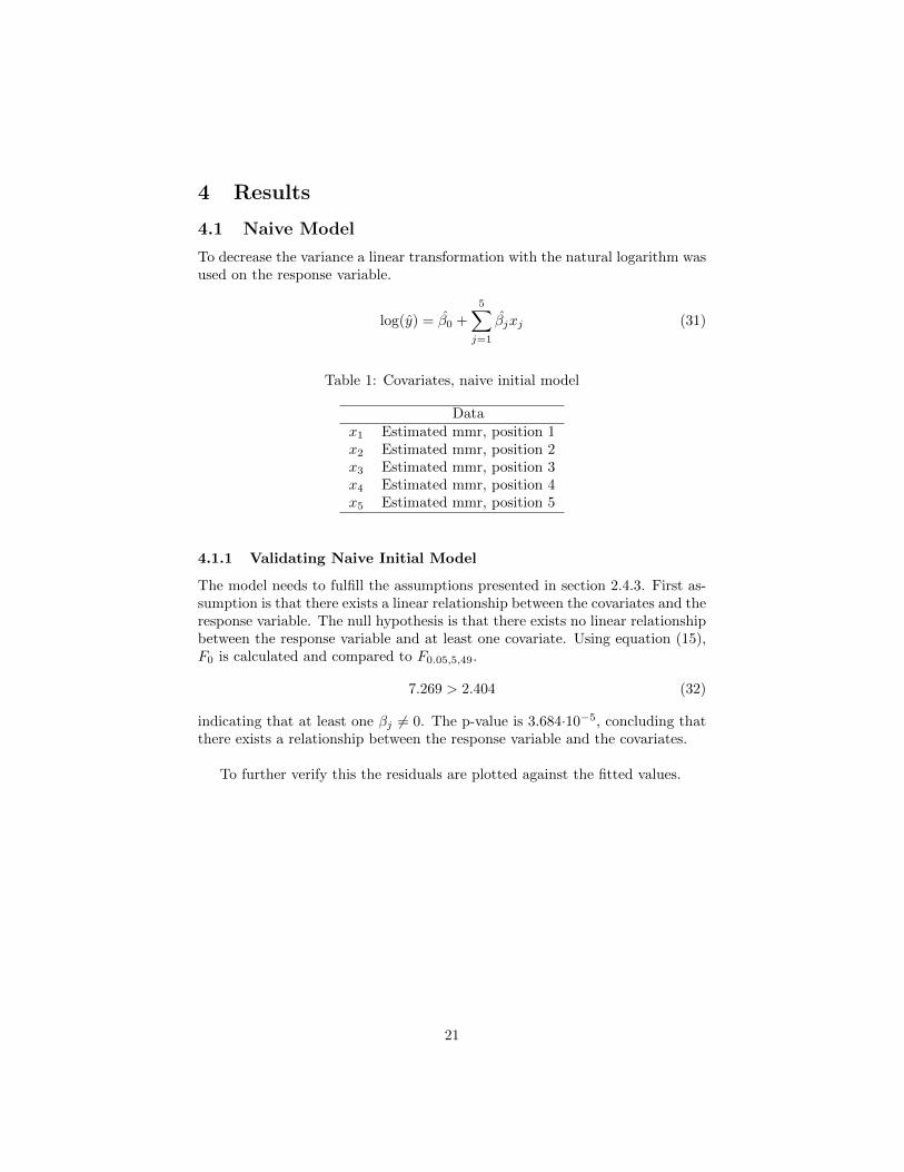
Figure 4: Naive initial model, residual vs fitted

Figure 4 shows an almost straight line that has a small deviation towardsthe end. This could be a result of a small sample size of only 55 observations.The plot is interpreted to show a linear relationship.

The second assumption is that the errors are normally distributed. Onemethod to verify this assumption is to use the normal Q-Q plot [12]. The plotshows the residuals plotted against the quantiles. If the errors are normallydistributed the points in the plot should form a straight line.

Figure 5: Naive initial model, Normal Q-Q

A straight line with a small deviation in the end is shown in figure 5. It issufficiently normally distributed to continue evaluate the naive initial model.

The third assumption is that the errors have a constant variance. The scale-location plot shows the spread of the points across the predicted values range. If

22

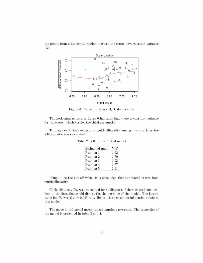
the points form a horizontal random pattern the errors have constant variance[12].

Figure 6: Naive initial model, Scale-Location

The horizontal pattern in figure 6 indicates that there is constant variancefor the errors, which verifies the third assumption.

To diagnose if there exists any multicollinearity among the covariates theVIF statistic was calculated.

Table 2: VIF, Naive initial model

Estimated mmr VIFPosition 1 1.62Position 2 1.70Position 3 1.92Position 4 1.77Position 5 2.11

Using 10 as the cut off value, it is concluded that the model is free frommulticollinearity.

Cooks distance, Di, was calculated for to diagnose if there existed any out-liers in the data that could distort the the outcome of the model. The largestvalue for Di was D30 = 0.085 < 1. Hence, there exists no influential points inthis model.

The naive initial model meets the assumptions necessary. The properties ofthe model is presented in table 3 and 4.

23

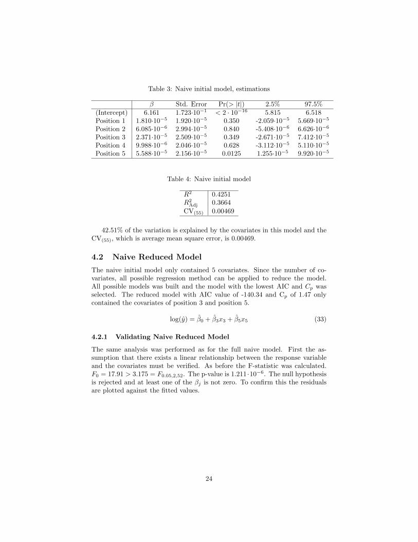
Table 3: Naive initial model, estimations

β Std. Error Pr(> |t|) 2.5% 97.5%(Intercept) 6.161 1.723·10−1 < 2 · 10−16 5.815 6.518Position 1 1.810·10−5 1.920·10−5 0.350 -2.059·10−5 5.669·10−5

Position 2 6.085·10−6 2.994·10−5 0.840 -5.408·10−6 6.626·10−6

Position 3 2.371·10−5 2.509·10−5 0.349 -2.671·10−5 7.412·10−5

Position 4 9.988·10−6 2.046·10−5 0.628 -3.112·10−5 5.110·10−5

Position 5 5.588·10−5 2.156·10−5 0.0125 1.255·10−5 9.920·10−5

Table 4: Naive initial model

R2 0.4251R2

Adj 0.3664

CV(55) 0.00469

42.51% of the variation is explained by the covariates in this model and theCV(55), which is average mean square error, is 0.00469.

4.2 Naive Reduced Model

The naive initial model only contained 5 covariates. Since the number of co-variates, all possible regression method can be applied to reduce the model.All possible models was built and the model with the lowest AIC and Cp wasselected. The reduced model with AIC value of -140.34 and Cp of 1.47 onlycontained the covariates of position 3 and position 5.

log(y) = β0 + β3x3 + β5x5 (33)

4.2.1 Validating Naive Reduced Model

The same analysis was performed as for the full naive model. First the as-sumption that there exists a linear relationship between the response variableand the covariates must be verified. As before the F-statistic was calculated.F0 = 17.91 > 3.175 = F0.05,2,52. The p-value is 1.211 ·10−6. The null hypothesisis rejected and at least one of the βj is not zero. To confirm this the residualsare plotted against the fitted values.

24

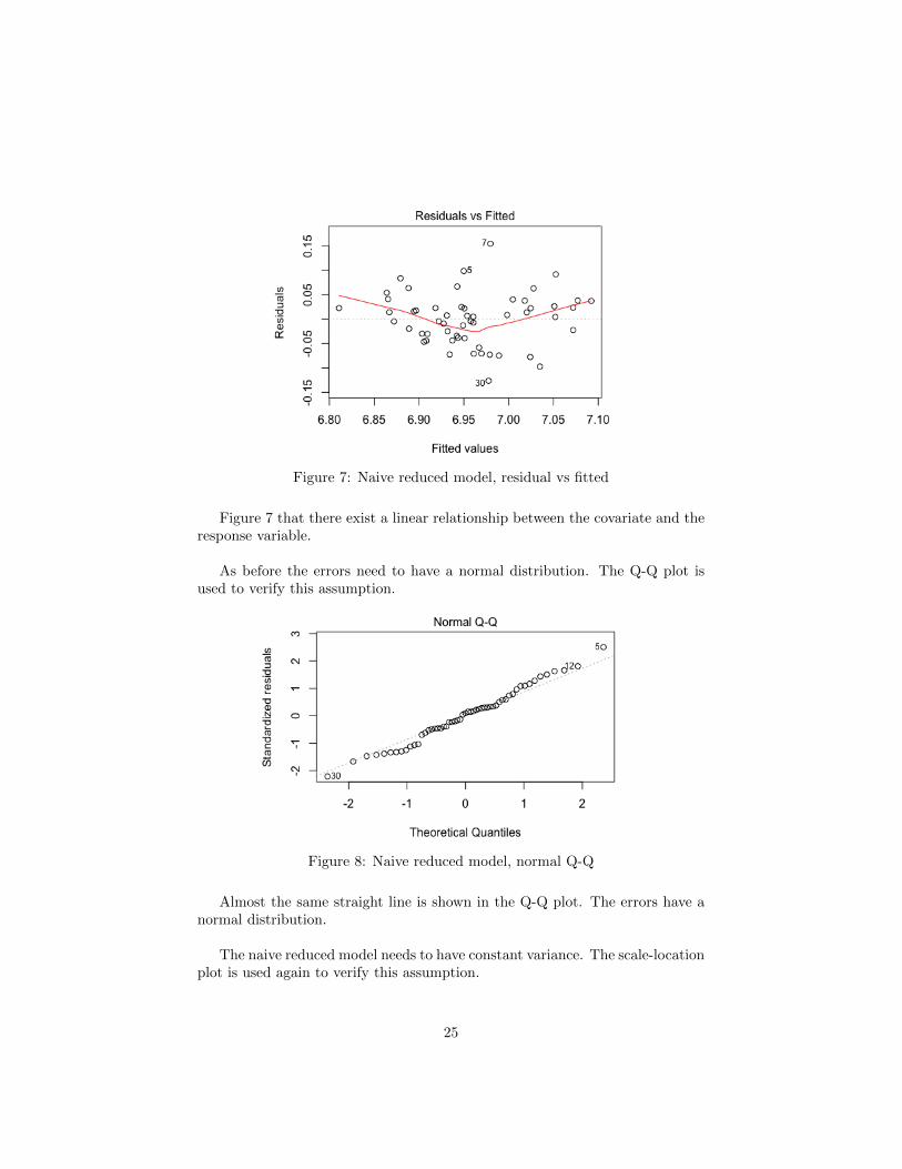
Figure 7: Naive reduced model, residual vs fitted

Figure 7 that there exist a linear relationship between the covariate and theresponse variable.

As before the errors need to have a normal distribution. The Q-Q plot isused to verify this assumption.

Figure 8: Naive reduced model, normal Q-Q

Almost the same straight line is shown in the Q-Q plot. The errors have anormal distribution.

The naive reduced model needs to have constant variance. The scale-locationplot is used again to verify this assumption.

25

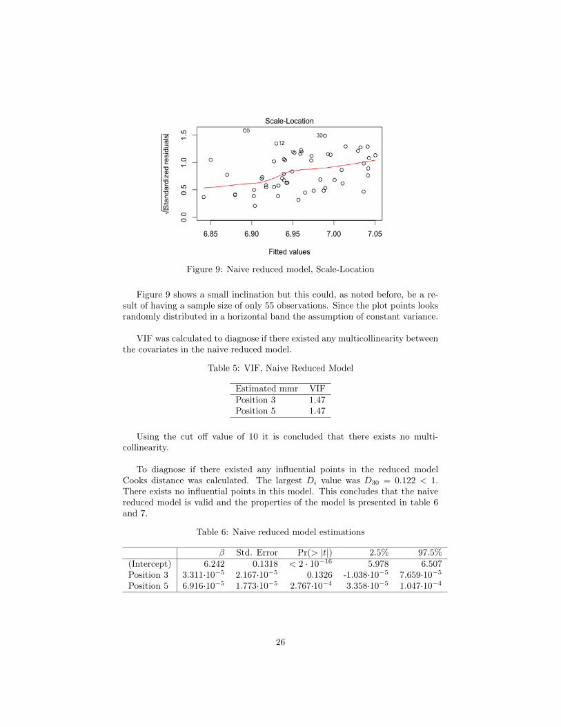
Figure 9: Naive reduced model, Scale-Location

Figure 9 shows a small inclination but this could, as noted before, be a re-sult of having a sample size of only 55 observations. Since the plot points looksrandomly distributed in a horizontal band the assumption of constant variance.

VIF was calculated to diagnose if there existed any multicollinearity betweenthe covariates in the naive reduced model.

Table 5: VIF, Naive Reduced Model

Estimated mmr VIFPosition 3 1.47Position 5 1.47

Using the cut off value of 10 it is concluded that there exists no multi-collinearity.

To diagnose if there existed any influential points in the reduced modelCooks distance was calculated. The largest Di value was D30 = 0.122 < 1.There exists no influential points in this model. This concludes that the naivereduced model is valid and the properties of the model is presented in table 6and 7.

Table 6: Naive reduced model estimations

β Std. Error Pr(> |t|) 2.5% 97.5%(Intercept) 6.242 0.1318 < 2 · 10−16 5.978 6.507Position 3 3.311·10−5 2.167·10−5 0.1326 -1.038·10−5 7.659·10−5

Position 5 6.916·10−5 1.773·10−5 2.767·10−4 3.358·10−5 1.047·10−4

26

Table 7: Naive reduced model properties

R2 0.4078R2

Adj 0.3851

CV(55) 0.00442

4.3 Extended Initial Model

The extended model includes more covariates than the naive model. The esti-mated mmr have been summarized to a single value. The rest of the covariatesare explained in section 3.2.3. The Chinese region is used as a benchmark forthe dummy variables. The response variable was transformed using the naturallogarithm to make the model more linear.

log(y) = β0 +

11∑j=1

βjxj (34)

Table 8: Covariates, extended initial model

Datax1 Total mmr sumx2 Mmr differencex3 Gamesx4 Age of the organizationx5 Region North America (dummy)x6 Region South America (dummy)x7 Region Europe (dummy)x8 Region CIS (dummy)x9 Region Southeast Asia (dummy)x10 Sum of nationalitiesx11 Total amount of players

4.3.1 Validating Extended Initial Model

The model needs to fulfill the same assumptions as the naive model before it canbe reduced. The same line of reasoning was applied as the naive initial model,therefor only the results and comments about the results will be presented.

F0 = 5.604 > 2.019502 = F0.05,11,43 (35)

27

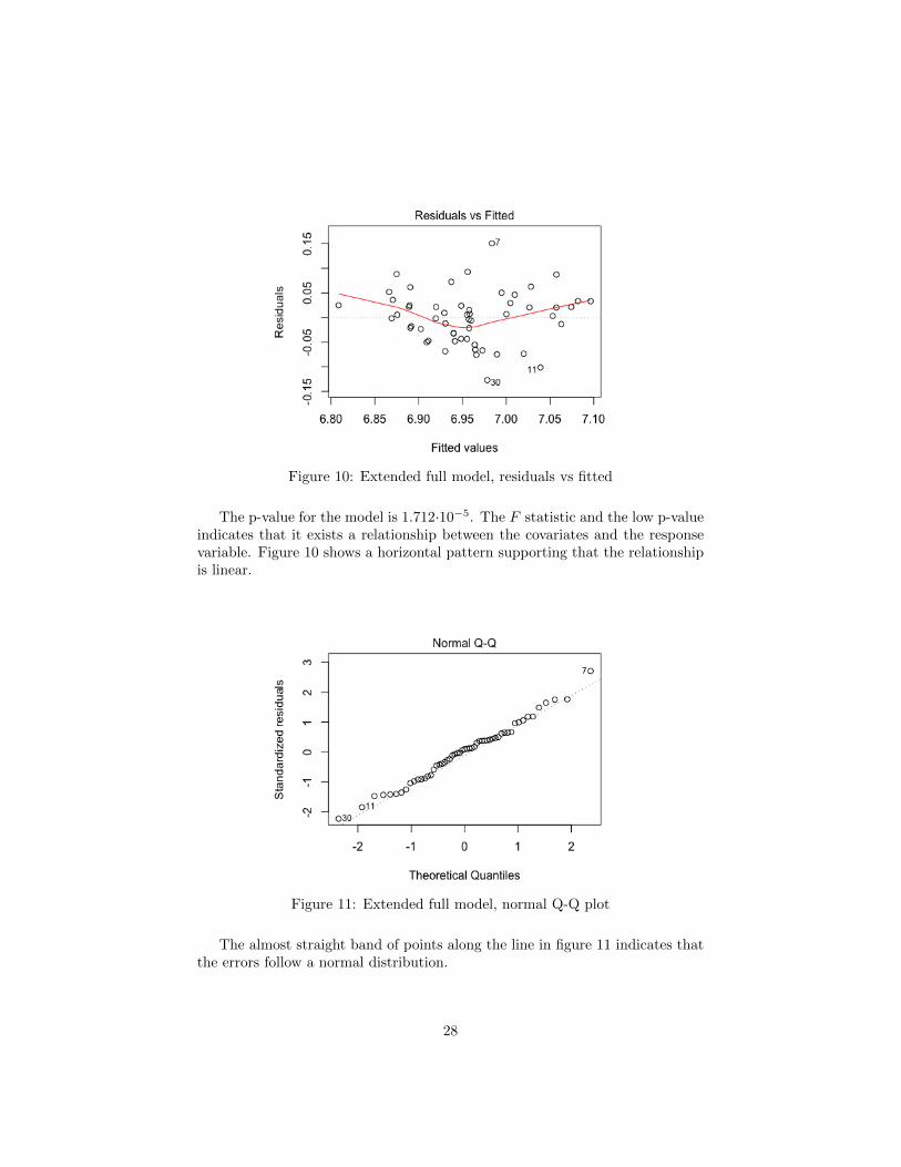
Figure 10: Extended full model, residuals vs fitted

The p-value for the model is 1.712·10−5. The F statistic and the low p-valueindicates that it exists a relationship between the covariates and the responsevariable. Figure 10 shows a horizontal pattern supporting that the relationshipis linear.

Figure 11: Extended full model, normal Q-Q plot

The almost straight band of points along the line in figure 11 indicates thatthe errors follow a normal distribution.

28

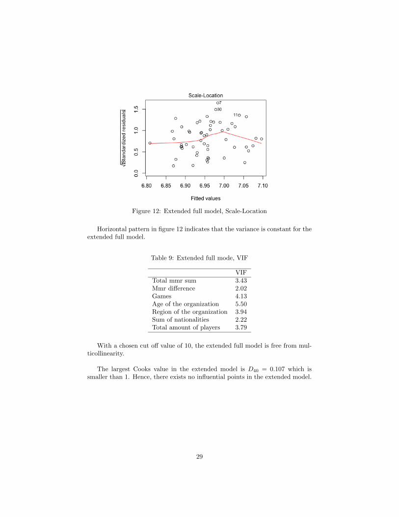
Figure 12: Extended full model, Scale-Location

Horizontal pattern in figure 12 indicates that the variance is constant for theextended full model.

Table 9: Extended full mode, VIF

VIFTotal mmr sum 3.43Mmr difference 2.02Games 4.13Age of the organization 5.50Region of the organization 3.94Sum of nationalities 2.22Total amount of players 3.79

With a chosen cut off value of 10, the extended full model is free from mul-ticollinearity.

The largest Cooks value in the extended model is D40 = 0.107 which issmaller than 1. Hence, there exists no influential points in the extended model.

29

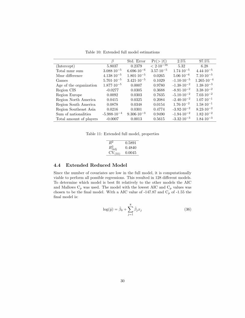
Table 10: Extended full model estimations

β Std. Error Pr(> |t|) 2.5% 97.5%(Intercept) 5.8037 0.2379 < 2·10−16 5.32 6.28Total mmr sum 3.088·10−5 6.696·10−6 3.57·10−5 1.74·10−5 4.44·10−5

Mmr difference 4.138·10−5 1.801·10−5 0.0265 5.06·10−6 7.10·10−5

Games 5.701·10−5 3.421·10−5 0.1029 -1.10·10−5 1.265·10−4

Age of the organization 1.877·10−5 0.0007 0.9780 -1.38·10−2 1.38·10−3

Region CIS -0.0277 0.0305 0.3688 -8.91·10−2 3.38·10−2

Region Europe 0.0092 0.0303 0.7635 -5.10·10−2 7.03·10−2

Region North America 0.0415 0.0325 0.2084 -2.40·10−2 1.07·10−1

Region South America 0.0878 0.0348 0.0154 1.76·10−2 1.58·10−1

Region Southeast Asia 0.0216 0.0301 0.4774 -3.92·10−2 8.23·10−2

Sum of nationalities -5.988·10−4 9.306·10−3 0.9490 -1.94·10−2 1.82·10−2

Total amount of players -0.0007 0.0013 0.5615 -3.32·10−3 1.84·10−3

Table 11: Extended full model, properties

R2 0.5891R2

Adj 0.4840

CV(55) 0.0045

4.4 Extended Reduced Model

Since the number of covariates are low in the full model, it is computationallyviable to perform all possible regressions. This resulted in 128 different models.To determine which model is best fit relatively to the other models the AICand Mallows Cp was used. The model with the lowest AIC and Cp values waschosen to be the final model. With a AIC value of -147.87 and Cp of -1.55 thefinal model is:

log(y) = β0 +

8∑j=1

βjxj (36)

30

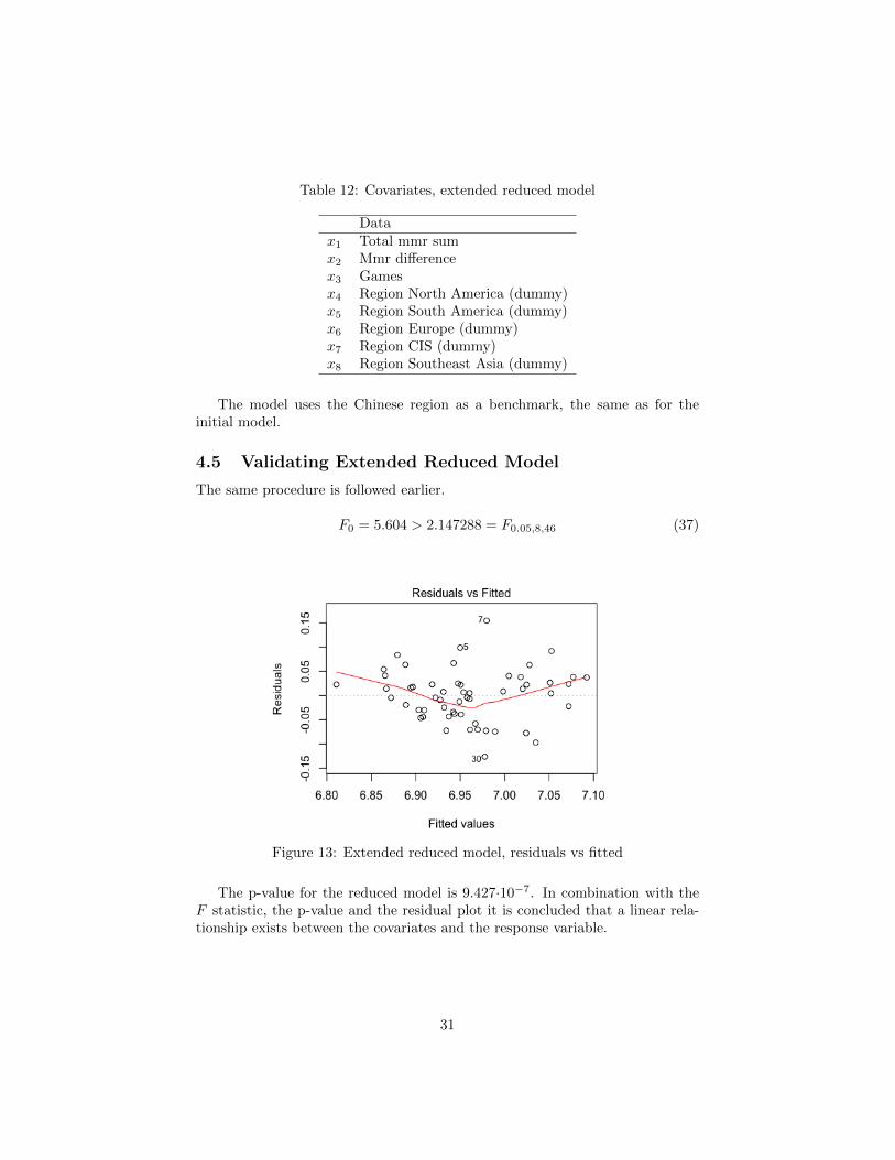
Table 12: Covariates, extended reduced model

Datax1 Total mmr sumx2 Mmr differencex3 Gamesx4 Region North America (dummy)x5 Region South America (dummy)x6 Region Europe (dummy)x7 Region CIS (dummy)x8 Region Southeast Asia (dummy)

The model uses the Chinese region as a benchmark, the same as for theinitial model.

4.5 Validating Extended Reduced Model

The same procedure is followed earlier.

F0 = 5.604 > 2.147288 = F0.05,8,46 (37)

Figure 13: Extended reduced model, residuals vs fitted

The p-value for the reduced model is 9.427·10−7. In combination with theF statistic, the p-value and the residual plot it is concluded that a linear rela-tionship exists between the covariates and the response variable.

31

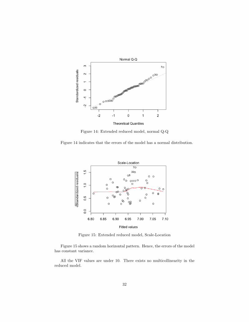
Figure 14: Extended reduced model, normal Q-Q

Figure 14 indicates that the errors of the model has a normal distribution.

Figure 15: Extended reduced model, Scale-Location

Figure 15 shows a random horizontal pattern. Hence, the errors of the modelhas constant variance.

All the VIF values are under 10. There exists no multicollinearity in thereduced model.

32

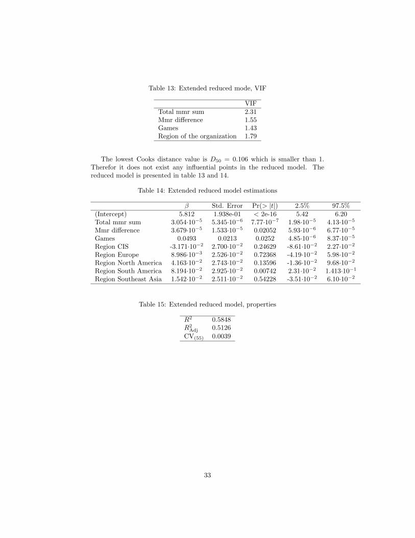
Table 13: Extended reduced mode, VIF

VIFTotal mmr sum 2.31Mmr difference 1.55Games 1.43Region of the organization 1.79

The lowest Cooks distance value is D50 = 0.106 which is smaller than 1.Therefor it does not exist any influential points in the reduced model. Thereduced model is presented in table 13 and 14.

Table 14: Extended reduced model estimations

β Std. Error Pr(> |t|) 2.5% 97.5%(Intercept) 5.812 1.938e-01 < 2e-16 5.42 6.20Total mmr sum 3.054·10−5 5.345·10−6 7.77·10−7 1.98·10−5 4.13·10−5

Mmr difference 3.679·10−5 1.533·10−5 0.02052 5.93·10−6 6.77·10−5

Games 0.0493 0.0213 0.0252 4.85·10−6 8.37·10−5

Region CIS -3.171·10−2 2.700·10−2 0.24629 -8.61·10−2 2.27·10−2

Region Europe 8.986·10−3 2.526·10−2 0.72368 -4.19·10−2 5.98·10−2

Region North America 4.163·10−2 2.743·10−2 0.13596 -1.36·10−2 9.68·10−2

Region South America 8.194·10−2 2.925·10−2 0.00742 2.31·10−2 1.413·10−1

Region Southeast Asia 1.542·10−2 2.511·10−2 0.54228 -3.51·10−2 6.10·10−2

Table 15: Extended reduced model, properties

R2 0.5848R2

Adj 0.5126

CV(55) 0.0039

33

4.6 Model Comparison and Analysis

All models are summarized in a single table with their features.

Table 16: Model comparisons

Naive Initial Model Naive Reduced ModelAIC -135.97 -140.34Cp 6.00 1.47R2 0.4251 0.4078R2

Adj 0.3664 0.3851

CV(55) 0.0047 0.0044Extended Initial Model Extended Reduced Model

AIC -142.44 -147.87Cp 4.00 -1.55R2 0.5891 0.5848R2

Adj 0.4840 0.5126

CV(55) 0.0045 0.0039

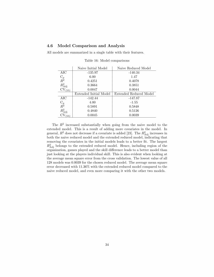
The R2 increased substantially when going from the naive model to theextended model. This is a result of adding more covariates in the model. Ingeneral, R2 does not decrease if a covariate is added [23]. The R2

Adj increases inboth the naive reduced model and the extended reduced model, indicating thatremoving the covariates in the initial models leads to a better fit. The largestR2

Adj belongs to the extended reduced model. Hence, including region of theorganization, games played and the skill difference leads to a better model thanjust looking at the players individual skill. This is also evident when looking atthe average mean square error from the cross validation. The lowest value of all128 models was 0.0039 for the chosen reduced model. The average mean squareerror decreased with 11.36% with the extended reduced model compared to thenaive reduced model, and even more comparing it with the other two models.

34

5 Discussion

The naive model showed that the individual skill of the players could be usedto predict the performance of the team. In the extended model the variable forskill used was the total individual skill instead of a covariate for each individualplayer. This was due to the fact that the data sample was limited in size andhaving five covariates representing individual skill was deemed suboptimal.

The result of the extended model shows that the number of nationalitiespresent in the team does not have a significant effect on the teams performance.The covariate for the total number of nationalities had a p-value close to 0.95and was therefore removed from the model. This does not mean that culturaldifferences and language barriers can’t impact a teams performance since peoplefrom different countries can have languages in common. Due to a small samplesize of 55 teams we can not examine the effect of language barriers since mostprofessional teams have members speaking the same languages.

The study does not include the players age, which is quantifiable, since it isnot stored in the Steam database. We tried to collect the age of all the playersmanually through different websites but the Dota 2 scene is too immature tostore accurate information of that kind, compared to football for example whereage, height and weight can be found on sport sites containing player data. A lotof the information regarding Dota 2 is still stored in wiki-sites like liquidpedia.

In Project Aristotle the key findings were factors that relates to the socialdynamics and corporate culture of the groups and teams. Our research andmodel focused to more easily quantifiable factors. That is because we chose tostudy factors that are more available to an outside observer. In order to studythe internal social dynamics of the Dota 2 teams we would need to do as vastdata collection project and survey teams from all around the world. Google re-searched their own teams while we would have to study competing teams fromdifferent organizations which we believe would only add to the difficulty. Dueto the scope of such a project and the possible problems that could arise such aslanguage barriers and teams not wanting to answer surveys regarding internalsocial dynamics we deemed that it was not possible for us hence we insteadused publicly available data. We do however believe that the social dynamicsfactors put forward by Project Aristotle could be helpful in modeling the skilland performance of Dota 2 teams. The factors psychological safety and depend-ability could possibly be very helpful since Dota 2 is a complex game with manydifferent strategies and teammates need to be able to trust each other and beable to speak their mind without being seen as ignorant, incompetent, negative,or disruptive if they want to be able to compete at the highest levels. Structureand clarity in terms of setting up achievable goals for the team is also factorsthat can help the success of a team. The meaning and impact of work howevermight not be as significant in professional gaming since it is much less abstractthen for example a big research project or preforming a highly specialized task

35

so the players should be able to see the bigger picture of their work much easier.Also worth noting is that while the researchers of Project Aristotle found thatindividual performance of team members were not significantly connected withteam effectiveness we found that the variable individual skill had significant ex-planatory power for the Dota 2 teams performance.

The research on both the Olympics and E-Sport found evidence to supportthe thesis that regional differences has an effect on the performance of athletes.While GDP and population was deemed to be the most influential factors whenit comes to traditional sport the same did not hold true for E-Sport. The factthat a nation’s GPD was significant for traditional sport but not for E-Sportcan possibly be explained by comparing the needs of traditional sport and E-Sport respectively. While traditional sport at the Olympic level has a need forworld class training facilities, E-Sport participation costs are much lower. TheOlympics is also more regulated then E-Sport. It requires a national Olympiccommittee that can work together with the International Olympic Committeein order to be eligible to compete and to determine the number of athletes anation are allowed to send. No such governing body exists for E-Sport whichlikely helps keep the participation costs low. For the Olympics a host nationadvantage was noted, we did not examine whether such an affect is present forDota 2 as well. If a host nation advantage exists for Dota 2 we believe that theeffect of it would have been greater if we had chosen a monetary measurementto represent the team’s success since most of the large Dota 2 tournaments areplayed in North America. Since we instead chose Elo rating which is not affectedby the money at stake at a given tournament, host nation advantage might nothave been as important for the model.

36

6 Conclusion

It is possible to create a linear fit both from the naive model and from theextended model. The naive model resulted in a worse fit than the extendedmodels. This indicates that it is reasonable to take the nationality of the orga-nization and the experience the organization into account along with the playerscombined estimated skill and skill difference.

The extended reduced model explains 58.48% of the variation in the data.Dota 2 is a team-based game and the outcome depends on how well the playerscan perform in the circumstances provided and the preparations leading up tothe game. The factors in the result are connected to the preparations since theyare not circumstantial. The p-value for matches is 0.1029, it is not possible toreject the null hypothesis for the covariate but including it leads to a betterestimation. In the extended reduced model all coefficients, except the dummyvariables, are positive. Hence, it is evident that the higher the estimated skillthat the players have combined, the more matches the organization have playedand the larger skill difference all have a positive effect on the teams rating. Withthe exception that the skill difference can be large but if the cause is that one ormore players have an estimated skill bellow the average professional estimatedskill, the teams combined skill will suffer. Therefor a large skill range is notnecessarily a good thing for the team.

Using the Chinese region as the benchmark the study finds that all otherregions except CIS predicts a better performance. The p-values for the differentregions seen in table 10 is high. Region Europe has a p-value of 0.76 so we can’treject the null hypothesis that there is no performance difference between thetwo regions. Region South America has the lowest p-value for the regions at0.015 which makes us believe that regional differences might still be a factor.The team distribution shows that over a third of the teams in the data arefrom China. This gives the study more detailed information about the Chineseteams while the other countries lack the same detail due to the small samplesize. Future research in this area could be to attempt to explain the regionaldifferences that was observed. These regional differences can possibly be ex-plained by examining demographic and economical factors.

For future research a more refined model could be obtained by looking atall registered teams in the Steam database, including amateur teams and teamsthat only participated in one competition, usually the International qualifiers.The soft factors found in Project Aristotle could also be interesting to examineto see how factors related to group dynamics can predict performance.

37

References

[1] Daniel K. N. Johnson Ayfer Ali. “A Tale of Two Seasons: Participationand Medal Counts at the Summer and Winter Olympic Games”. In: (29October 2004). doi: https://doi.org/10.1111/j.0038-4941.2004.00254.x.

[2] Meghan R. Busse Andrew B. Bernard. “Who Wins the Olympic Games:Economic Resources and Medal Totals”. In: Review of Economics andStatistics (February 2004). url: https://www.colorado.edu/Economics/courses/maskus/8209/bernard_olympics.pdf.

[3] Michael Roberto Richard M.J. Bohmer and Amy C. Edmondson. “Fac-ing Ambiguous Threats”. In: Harvard Business Review (November 2006).url: https://hbr.org/2006/11/facing-ambiguous-threats.

[4] Stewart Brand. SPACEWAR Fanatic Life and Symbolic Death Amongthe Computer Bums. url: http://www.wheels.org/spacewar/stone/rolling_stone.html. (accessed:6.05.2018).

[5] Ayfer Ali Daniel K. N. Johnson. “Coming to Play or Coming to Win:Participation and Success at the Olympic Games”. In: Wellesley Col-lege Dept. of Economics Working Paper No. 2000-10 (2 Nov 2000). url:https://papers.ssrn.com/sol3/papers.cfm?abstract_id=242818.

[6] Esports Earnings. Esports Earnings. url: https://www.esportsearnings.com/players. (accessed:6.05.2018).

[7] Esports Earnings. Esports Earnings. url: https://www.esportsearnings.com/games. (accessed:6.05.2018).

[8] Gamasutra. Analysis: Defense of the Ancients - An Underground Revolu-tion. url: https://web.archive.org/web/20120510135818/http://www.gamasutra.com/view/news/109814/Analysis_Defense_of_the_

Ancients__An_Underground_Revolution.php. (accessed:6.05.2018).

[9] Mark E. Glickman. A Comprehensive Guide To Chess Ratings. Interna-tional Series of Monographs on Physics. Harvard University, 1981.

[10] Google. Project Aristotle. url: https : / / rework . withgoogle . com /

guides/understanding-team-effectiveness/steps/introduction/.(accessed: 24.04.2018).

[11] Gareth R. Jones. “Task Visibility, Free Riding, and Shirking: Explainingthe Effect of Structure and Technology on Employee Behavior”. In: TheAcademy of Management Review 9 (October 1984), pp. 684–695. url:http://www.jstor.org/stable/258490.

[12] Bommae Kim. Understanding Diagnostic Plots for Linear Regression Anal-ysis. url: http://data.library.virginia.edu/diagnostic-plots/.(accessed: 24.04.2018).

[13] Harald Lang. Elements of Regression Analysis. KTH Mathematics, 2016.

38

[14] Newzoo. newzoo 2018 global esports market report. url: https://asociacionempresarialesports.es/wp- content/uploads/newzoo_2018_global_esports_market_

report_excerpt.pdf. (accessed:6.05.2018).

[15] Marina Oskolkova Petr Parshakov. “Success in eSports: Does CountryMatter?” In: National Research University Higher School of Economics(January 2016). doi: 10.13140/RG.2.1.3723.9445.

[16] Bruce N. Pfau. “How an Accounting Firm Convinced Its Employees TheyCould Change the World”. In: Harvard Business Review (October 2015).url: https://hbr.org/2015/10/how-an-accounting-firm-convinced-its-employees-they-could-change-the-world.

[17] Wade D. Pfau. “Predicting the Medal Wins by Country At the 2006 Win-ter Olympic Games: An Econometrics Approach”. In: The Korea Eco-nomic Review 22 (Winter 2006). url: https://papers.ssrn.com/sol3/papers.cfm?abstract_id=1267529.

[18] Hal Stern. “Are all linear paired comparison models empirically equiv-alent?” In: Mathematical Social Sciences 23 (1992), pp. 103–117. doi:https://doi.org/10.1016/0165-4896(92)90040-C.

[19] Gareth James Daniela Witten Trevor Hastie Robert Tibshirani. An Intro-duction to Statistical Learning with Applications in R. Springer Texts inStatistics. Springer, 2013. isbn: 9781461471370.

[20] Valve. Dota 2 Homepage. url: https://www.dota2.com/international/overview/. (accessed: 24.04.2018).

[21] Valve. Dota 2 International Announcement. url: https://www.dota2.com/international/announcement/. (accessed: 2.05.2018).

[22] Valve. Dota 2 mmr blog. url: http://blog.dota2.com/2013/12/

matchmaking/. (accessed: 2.05.2018).

[23] Douglas C. Montgomery Elizabeth A. Peck G. Geoffery Vining. Intro-duction to Linear Regression Analysis. Wiley Series in Probability andStatistics. John Wiley & Sons Inc, 2012. isbn: 9780470542811.

39

A Appendix

Figure 16: Distribution of countries

Teams

1. Virtus Pro

2. Team Secret

3. LGD Gaming

4. Evil Geniuses

5. SG E-sport Team

6. Team Liquid

7. VGJ Thunder

8. Fnatic

9. Newbee

10. OG

11. Invictus Gaming

12. Complexity Gam-ing

13. Pain Gaming

14. Optic Gaming

15. Vici Gaming

16. Mineski

17. TNC Predator

18. Team Spirit

19. Keen Gaming

20. Vega Squadron

21. Rock Young

22. Rock Gaming

23. Team Empire

24. Team Kinguin

25. Execration

26. Immortals

27. LGD.ForeverYoung

28. Digital Chaos

29. Vici Gaming Po-tential

30. IG Vitality

31. Skiter Evil

32. The Final Tribe

33. Geem Fam

34. Newbee Young

35. Effect

36. Team Braveheart

37. Eclipse

38. Ehome

39. Team Waoo

40. Mousesports

41. Mad King E-sport

42. T Show

43. Keen Gaming Lu-minous

44. VGJ Storm

45. Natus Vincere

46. Infamous

47. Sacred

48. Happy Feet

49. BOOM ID

50. Alliance

51. Clutch Gamers

52. CDEC Gaming

53. Gambit E-sport

54. Midas Club

55. Team Max

40