Embed Size (px)
Citation preview

Analyzing Effects of Stringlines on Initial Smoothness of Concrete Pavements
By
Bernard Igbafen Izevbekhai, P.E.
B.Eng. Hons Civil, University Of Benin, Benin City Nigeria 1983
M.Eng. Civil/ Structural Eng University of Benin, Benin City, Nigeria 1987
MS Infrastructure Systems Engineering, University of Minnesota
Center for the Development of Technological Leadership. 2004
Being a Discussion of the Paper Titled
“Stringline Effects on Concrete Pavement Construction”
November 2008

Abstract
This reviews the paper titled “Effects of stringline on Concrete Pavement Construction, Published
by the Transportation Research Journal, Transportation Research Record Issue Number 1900 of
2000. The paper authors discussed traditional slip form paving construction in which a sensor in
contact with the stringline determines the finished surface. These stringlines are subject to catenaries
and survey errors in regular paving. Additionally they are subject to errors due to chord effects that
occur when stringline paving is done on a vertical curve.
Reviewer summarizes the paper, elucidates the major ride quality metrics and accentuates the
process of addition of profilograms mentioned by authors. Reviewer further discusses a case study
of a classic pavement project that exhibited chatter phenomena to systematically accentuate how
stringlines, joint intervals, warp and curl as well as their synergy influence the measured ride
quality. The International Roughness Index (IRI) profilograms for the component dominant
wavelengths are fitted in a curve to determine correlation to the measured IRI first in the spatial and
next in the spectral domain.
Fourier Transform Moduli for component dominant wavelengths were more correlated to that of the
measured frequency than the IRI in the spatial domain. The stringline effect were also validated
although the paper made little reference to other paving features of equal importance and post
pavement built-in warp-and-curl that are of equal and occasionally greater relevance to ride quality.

1) INTRODUCTION
The Paper under review was written Authors Rasmussen, R.O; Karamihas, S.K; Cape, W.R., Chang,
G.K., and Guntert, R.M. titled “Stringline Effects on Concrete Pavement Construction” is being
reviewed. The Paper is hereinafter referred to as the paper and the authors (Rassmussen et al) are
herein after referred to as the Authors and for avoidance of doubt, the latter term is not used for the
reviewer. Instead the term “review and reviewer” are reserved for this exercise.
Objectives of the Review
This review primarily accentuates intrinsic issues implicit in the paper. It therefore clearly
defines the terms used, expatiates on the paving practices and use of stringlines, enunciating
ride quality is actually affected by stringlines.
It examines other studies germane to the effect of stringlines on ride quality and identifies and
discusses relevant areas not covered by authors that elucidate authors’ objectives
The review discusses a case study of Minnesota Department of Transportation (Mn/DOT)
Highway 59 project, a classic case of “Chatter Phenomena” caused by loose stringlines. The
review elucidates the spectral content in US Highway 59 project in Morris Minnesota caused
by stringlines, joints and synergistic effects of both.
It consequently advocates a study of Pavement Surface Characteristics in the frequency domain
(in preference to or in addition to the spatial domain) towards a better understanding of
causative and associative parameters of pavement smoothness.
2) SUMMARY OF THE PAPER
The paper identifies and discusses the use of stringlines as a sensor guide for establishing the finished
surface of a concrete paving. Authors (1) noted how the current effort of States and Industry towards
smoother pavements and better measurement techniques and metrics had resulted in some states
transitioning to the International Roughness Index (IRI). Hitherto most states used the Profile Index
(PI) as the metric for pavement smoothness. Authors had neither defined IRI and PI nor mentioned the
difference in the response spectra or multiplier algorithm of each of these metrics. According to
authors (1) stringlines were introduced to improve pavement smoothness by sensing a stringline to a
remarkable degree of precision. This is arguably counterproductive.
The paper identified 3 unique effects of stringlines as
The chord effect,
The sag effect and
Survey errors
They (1) noted that of the 3, survey errors were the most pronounced. Chord effect is explained as the
outline of a chord instead of a smooth curve that should normally characterize a vertical curve. If the
radius is very large and the stringline support interval is small, chord effect error is minimized. When
the radius is large and the stringline support interval is large, there will be severe errors in the profile
due to the chord effect. The chord effect is idealized with a system if cable supports joined end to end
along a vertical curve and not maintaining the required curvature but a system of chords joined end to
end. The sag effect is caused by tension in the chord that is insufficient to render the string horizontal.
The resulting sag profile is dependent on the actual tension at the ends of the stringing process. The
survey effect is idealized in terms of a normally distributed set of deviations from the actual nodal
points of the stringline set up.
The paper goes further to quantify the effect of stringlines in terms of the percentage increase in
roughness due to the already identified causes. Authors then proceeded to demonstrate the effect of the
various error sources to quantify and compare their effect on pseudo randomly generated profiles and
vertical curves. They (1) generated pseudo random profiles with the procedure prescribed in
Appendix E NCHRP 353. This procedure integrates a series of random slopes generated by the
equation
Slope = 0 +z ( R )+ √(Gs/2∆)…………………………………2.1
Where z = Inverse of the normal Cumulative distribution based on R
R = A probability number between 0 and 1 dependent on the inverse of the normal cumulative
distribution
Gs = White Noise amplitude in ft (m)/cycle chosen as
∆ = Step size in ft or m… chosen as 0.5ft
They consequently generated the vertical cu4ves with the equation
E1= g1x+ (g2-g1)x2/2L………………………………………..2.2
Where g1= Starting Slope of the vertical curve
E1= Initial datum reference for the beginning of the vertical curve
x = Station with respect to the Start of vertical curve
L = Length of curve
Authors superimposed the randomly generated profile on the vertical curve. The curvature of the
vertical curve and its length are outside of the range that will cause huge vertical acceleration on the
quarter car. The authors thus obtained IRI values that are similar to that of the random profile on a
horizontal surface. The catenary due to stringlines was imposed on the vertical curve. The feature was
idealized in a format of discontinuous straight lines connected at every 25ft interval Thereafter, the
resulting profile was subjected to the IRI algorithm through a process that is later explained in this
review and IRI values were obtained for various corresponding values of g1 and g2. This resulted in a
family of values proven to be sensitive to g2-g1. Evidently, the higher the value of (│g2-g1 ,the higher
the percentage increase in IRI. Respective g1 and g2 values of 0 resulted in zero increase in IRI from
the smooth vertical curve and respective 0 and 2 resulted in a 5% increase compared to –8 and 8%that
resulted in a 171% increase in IRI. It must be noted that the corresponding increase in Ride number
was not that significant, not because of scaling difference but because of the dissimilar sensitivity
range and gain algorithms (6) for the chosen metric.
The process of addition of profilograms already discussed under chord effect was replicated in the
examination of sag effect. Authors also idealized the sag effect by imposing various sag profiles on a
vertical curve and computed the sensitivity of the IRI to these deviations from the curve. Percentage
increase in IRI ranged from 0 due to zero sag to 368 % increase in IRI due to an inch sag. To establish
the sag profile the sag was computed on the basis of the tension in the string measured.
To quantify the effect of Survey errors, authors generated errors of various standard deviations (SD)
from the stringline survey data. To build the factorial, authors generated survey errors in the nodes
(stringline supports) in a normal distribution ranging from zero to 0.5 inch with stringline stake interval
ranging from 10 to 50 ft. Corresponding IRI ranged from 0 to 383 %.
The paper limits application of these results to systems with single lasers and recognizes unstable
foundation wind effects, moisture and temperature changes are responsible for loose stringlines. They
also itemized other sources of errors including knot effect, interference effect, foundation effect and
wand lift effect.
Although authors referenced other sources of Stringline errors, reviewer observes the following are
equally impertinent sources of error.
Temperature variation during placement of the Concrete pavement. The inspectors try to
tighten stringlines just before paving and when slackness is observed during paving.
Unfortunately it is counterproductive to make adjustments on the stringline when paving had
already begun. This is because the surfaces paved after adjustment are in a different stringline
setting from the previous segments, thus causing unwarranted kinks in the profile.
Oversensitive Stringlines. Contractors in have alluded to the fact that over-sensitivity of the
traveling sensor is counterproductive. For instance, an over sensitive sensor, is adversely
affected by the enclosure of the stringline at the support that the sensor interprets as a bump.
3 STRINGLINES IN PAVEMENT CONSTRUCTION
Various vehicles respond to various surface profiles according to their natural frequencies, their sprung
masses, spring constants and dashpot constants. Although the international roughness index is a
standard measure of ride quality, the measurement is only as good as the degree to which the
equipment or ride algorithm responds to the preponderant frequency. The international roughness
index is designed to be more sensitive to certain frequencies than others in order to represent how the
rider feels. In addition to amplified response of the quarter car to certain frequencies, errors resulting
from any deviation from the smooth profile are only predictable to the degree of response of the
quarter car algorithm to that profile and the deviation from it.
In consequence when errors due to the paving operations are introduced to the pavement, features
certain wavelengths are amplified or attenuation of depending on where a wavelength or frequency fits
in the IRI multiplier shown above as above. To understand the concept of IRI multiplier, the basic ride
(or roughness) metric deserves a good definition.
The International Roughness index has been variously defined from the simple description of what the
name implies (a roughness Index) to the definition in the frequency domain. The international
roughness index has been defined (1) as the average rectified velocity (ARV) of the Slope Power
Spectrum Density of the profilogram. This definition recognizes implicitly the ramification of

profilograms into various frequencies and amplitudes from which a slope, deflection or vertical
acceleration PSD can be plotted. The Slope PSD, Plotted against wavelength (or wave number or
frequency) has the dimension of ft/ cycle while the elevation PSD has the dimension of ft2-
ft/Cycle.
The IRI can therefore be graphically obtained from the Slope PSD. This is a cumbersome process that
software such as FHWA ProVAL and UMTRI Roadruf have facilitated. A ride profile can
consequently be idealized by Fourier transform or wavelet analysis but the latter 2 may not eliminate
the harmonic effects as ProVAL and Road RUF would. Alternately the transform algorithm may be
used in the computation as shown in equations 3.4 and 3.5.
Izevbekhai B.I. (2) discussed the effect of texture and joints on pavement roughness in his thesis titled
Optimization of Pavement Smoothness and Surface Texturing in Pavement Infrastructure at Center for
the Development of Technological Leadership (CDTL) University of Minnesota 2004. The thesis was
based on some test sections created in US Highway 212 in Bird Island. The Test sections were made of
adjacent yet concurrently finished segments that compared the textured finish to the untextured finish.
Results showed that joints and texture did contribute to the computed IRI. Additionally the thesis
discussed the friction-ride paradox and proposed an algorithm for incentives and penalties for good and
poor ride respectively. In retrospect, the sections were not examined for unusual hot spots associated
with string lines.
Karamihas and Sayers. (3) Little book of Profiling discussed the fundamentals of ride measurement
and defined many filters particularly “blanking bands” used in the PI metric but do not apply to IRI.
Smith K.L, Smith, K.D., Evans L.D., Hoerner, T.E., Darter M.I. in their report “Smoothness
Specification for Pavements” Final Report NCHRP 1-31 March 1997 discussed the effect of initial
ride quality of pavement performance concluded from nationwide data that pavements with initial high
smoothness remain smooth. This is a useful performance predictor re-enacting the fact that initial ride
quality is important in pavement practice.
Wilde W. J., Izevbekhai, B.I., and Krause, M.H. compared Profile Index and International Roughness
Index in Payment of Incentives in Pavement Construction (TRB 2007) Transportation Research
Records, discussed the various effects of paving activities and pavement joint spacing on IRI and PI.
In their paper, (3) they itemized the preponderant waveforms as emanating from
Joint spacing 15ft
Stringlines ((25ft)
Multiples especially 2 times the Stringline internodal spacing (50 ft)
According to Wilde Izevbekhai & Krause (5) regardless of the random profile generated, as long as it
was generated with the same input parameters to the random profile generator, the variability of the
ride statistics were very small for both the IRI and PI. It is concluded in consequence that the
percentage increase due to a waveform superposed on the profile is not arbitrary even if the general
process of profile generation appears to be. It is important to note that multiple random profiles,
generated with the same input parameters, produce profiles with very similar ride statistics. There are
predictable changes in the ride statistic when certain features are added to the random profile. The 15-
foot (4.6-m) wavelength content added to the random profiles caused large increases in IRI when
compared to the random profile (more than double), and the PI 0.0 statistic increased only about 70%.
Changes in the ride statistics due to catenary effects on the unmodified random profile were thus

accentuated. The 15-foot (4.6-m) wavelength has the largest impact on IRI and that the combination of
the 15-and 25-foot (4.6-m and 7.6-m) wavelengths has the largest impact on PI. 4 1 in/mi = 0.0158
m/km, Wilde, Izevbekhai, and Krause (5) also obtained the following results from their analysis
Random+15-ft upward catenary 104%
Random+15-ft downward catenary 106%
Random+15-ft sine wave 115%
Random+25-ft upward catenary 21%
Random+25-ft sine wave 22%
Random+50-ft upward catenary 9%
Random+50-ft sine wave 9% -3%
Random+15-ft and 25-ft upward catenaries 118% Increase over Random
Wilde Izevbekhai and Krause (5) also discussed the effect of added wavelengths on IRI and PI.
A second analysis was conducted to determine the effects of specific, individual wavelengths on ride
statistics. Based on the very small variation in ride statistics between the five random profiles, this
second analysis was only conducted using one of the random profiles. Figure 5 shows this sensitivity
of IRI and PI0.0 to individually added wavelengths. The subscript refers to the zero blanking band.
The analysis conducted added a sine wave of the specified wavelength to one of the random profiles
used in the previous analysis. Perera et al (6) showed the IRI and PI gain algorithm as in figures 3.2
and 3.3.Evident in figure 3.1 (5) is the respective response of PI and IRI with the 25 ft wavelength
addition causing increase in PI of 60% and 20%. The multiplier algorithm in figures 3.2 and 3.3
respectively for IRI and Ride number (which is same for PI) show a gain factor of 0.5 in IRI and 0.1 in
PI or RN.
.
Figure 3.1 Response and of IRI model to added frequency Figure 6: (After Wilde, Izevbekhai &
Krause)

Figure 3.2 Gain Algorithm for IRI (6)
Figure 3.3 Gain Algorithm for PI or RN (6)
Byrum R C (7). discussed :”Slab Curvature Detection In LTPP High-Speed Profilers, Developing
Predictive Models Using Generic Non-Linear Optimization”. In their paper, Byrum idealized slab
curvature and analyzed their effect on international roughness index. For any constant magnitude of
slab curvature, IRI increases exponentially with increasing slab length. Therefore, two pavement
sections, one with short joints and one with long joints, constructed in the same way under the same
environmental conditions could have significantly different initial IRI values if slab curvature
develops. This would not be the result of the contractor’s actions, but is the result of a design decision
put in place long before construction. This joint spacing effect should be considered in initial
smoothness specifications having very high smoothness requirements that can be affected by typical

locked in slab curvature values. He (7) also observed differences in Maximum slab curvature from
wheel path curvature. A road profiler moving at high speeds is measuring the “wheel path view” of
slab curvature. The curvature measured along a wheel path is a subdued and distorted image of the
maximum slab curvature.
According to Awashti and Singh (8), in their paper “On Pavement Roughness Indices” the simulated
profile (profilograms) can be expressed in the series
F (x) = (σ)( 2/N) 1/2
∫Σk=1 cos wkt 3.1
considering a Gaussian random process f (x) with mean zero and the spectral density function S( .
This process can be simulated by the way of the series.
Area under the PSD curve increases linearly as roughness increases
+
Where σ = ∫- s (w)dw 3.2
According to Awashti et al,(7) the PSD value (Gk) at any point k is given as
N-1
Xk = Σi=1 Xi e (-2 πik/N)
3.3
Gk = 2y/N/ * ( ABS Xk)2
3.4
and wk(k=1,2,......,N) are random variables identically distributed by the density function S(w) and
represents the PSD curve of the road profile, where y is sample interval; N, total number of sample
points; and Xk , the Fourier transformation of the sample points up to k, k being any point.
Figures 3.4 and 3.5 respectively show the stringline supported at 25 ft interval.

Figure 3.4 : Stringlines at 25 ft Interval. This is Typical
STRINGLINE SUPPORT
STRINGLINE
Figure 3.5: Stringlines In Close-Up

4 REVIEWER’S VALIDATION OF EFFECTS OF STRINGLINE ON PAVEMENT PROFILE
In this section Reviewer validates effect of stringlines by going through the process set forth in
NCHRP 335 appendix E (11) and reported by authors (1). This section studies the effect of stringline
on vertical curve to accentuate the chord effect identified by Rassmussen et al (1), the following
process was utilized.
Step 1: A field value of a vertical curve was generated, using the approach slope of 0.5 and the exit
slope of -0.6. Using an interval of 0.1ft, the vertical curve was generated. The formula used was g1X
The formula used was
E +g1X + (g2-g1) X2/2L……………………………………………………4.1
Where E is the datum elevation
g1 is approach slope
X is station with respect to the Cove
g2 is the departure slope
L is the length of curve
Step 2 . Similar curves were generated for the
vertical curve with stringlines and for the
vertical curve without stringline
For sag of 0.1ft, the Stringline catenary is idealized to be
F(x) = 0.1-SG*(ABS(SIN(3.14157 * X / INT ))))……………………………4.2
Where SG is the maximum sag due to loose stringlines
(SG is sag of the stringline
ABS (SIN(3.14157 *
X is the station
INT is stringline support interval.
The profile formed from equation 4.2 is a survey profile and not a ride profile. To convert it to a ride
profile we need to know how the quarter car will respond to that profile. The response profile of the
quarter car is the ride profile. This leads to the next step.
Step 3: Each of the 3 Profiles were exported into the raw ProVAL software and the resulting ASCII
file was saved as ERD files. The resulting Profile was analyzed for ride quality, PSD and ride statistics.
The resulting profiles and intrinsic properties are shown in figures 4.3 and 4.4.

Table 4.1 Vertical Curve Example
Eone= 0 INT=25 gone=-0.5 El=500 g2= -0.6 500
VC STR VC +STR VC STR VC +STR
0 0 0.1 0.1 1.3 -0.64814 0.083736 -0.5644
0.1 -0.04999 0.098743 0.048754 1.4 -0.69784 0.082498 -0.61535
0.2 -0.09996 0.097487 -0.00247 1.5 -0.74753 0.081262 -0.66626
0.3 -0.1499 0.096231 -0.05367 1.6 -0.79718 0.080029 -0.71715
0.4 -0.19982 0.094976 -0.10485 1.7 -0.84682 0.078799 -0.76802
0.5 -0.24973 0.093721 -0.156 1.8 -0.89644 0.077573 -0.81886
0.6 -0.2996 0.092467 -0.20714 1.9 -0.94603 0.07635 -0.86968
0.7 -0.34946 0.091215 -0.25825 2 -0.9956 0.075131 -0.92047
0.8 -0.3993 0.089964 -0.30933 2.1 -1.04515 0.073916 -0.97123
0.9 -0.44911 0.088714 -0.36039 2.2 -1.09468 0.072705 -1.02197
1 -0.4989 0.087467 -0.41143 2.3 -1.14418 0.071498 -1.07268
1.2 -0.59842 0.084978 -0.51344
Figure 4.3:Analysis of Stringline Chord Effect Using ProVAL Software

Table 4.2: Analysis - Ride Statistics Channel Title IRI (in/mi) PTRN (in/mi) RN
Stringline 45.5 51.7 4.39
Vertical Curve 8.9 24.5 4.70
String Line Imposed on Vertical Curve 49.6 59.7 4.30
Figure 4.3: PSD of Stringline Showing the highest harmonics at 25 ft wavelength
Generation of pavement surface is a common feature in pavement profilometry. The output obtained
provides information to a pavement designer who can minimize the effects of certain resonant
frequencies by providing adequate joint spacing, avoiding “finising-pan”-induced sinusoids and
ensuring tight stringlines as well as minimizing survey errors.
To convert a profile from the spatial to the frequency domain, the following process is required is
required
F (x) = an Σ sinw ωx + Σ bn Σ cos ωx …….. 4.1
Analysis - Power Spectral Density
Input Value Unit
PSD Calcu lation Slope
Use Point Reset No
Frequency Averaging No
Constant Frequency Interval 0.003048 cycle/ft
Pre-Processor Filter None

for all aperiodic signals (9)
Where f(x) is the profile and an and bn must be determined
f(x)= a0/2 + n=1 an cos nπx/L + n=1 bn sin nπx/L
= a0/2 + a1 cos πx/L + a2 cos 2πx/L + a3 cos 3πx/L + …….
+ b1 sin πx/L + b2 sin 2πx/L + b3 sin3πx/L+…. (4.3)
N-1
Xi = n=0 an cos ( 2πi/N) + bn sin ( 2πi/N) ……………………..(4.4)
Where an and bn are fourier coefficients 0,≤ ≤N/2)
xi is the profile elevation
Consequently
an = 1/N n=0 xi cos ( 2πi/N)
bn = 1/N n=0 xi sin ( 2πi/N)
w( )= /(N∆t) where
where w( ) is the frequency corresponding to and ∆t is the sampling interval
It can therefore be proven that removal of highly amplified wavelengths will improve pavement
smoothness.
N is number of profile elevation data points
The amplitudes represent maximum warp or maximum stringline sag. Evidently the degree of sag in a
truly truncated or normalized sine wave in which
fx = Abs ( Sag* Sin (πx / 25))…………. (4.5)
The process and effect of addition of wavelengths on a randomly generated profile (11) are shown in
appendix C and exemplified in section 5.

5 CASE STUDY OF A TYPICAL PAVEMENT EXHIBITING CHATTER PHENOMENA A largely biased set of data has been chosen for this project. This is the data from Minnesota Highway
59 in Morris. Reviewer ran a lightweight profiler on this project in 2004 in response to complaints
that the section was riding poorly. Riders experienced the “Chatter Phenomenon” on that pavement.
The ERD files were analyzed in PSD and the dominant wavelengths stood out at 25 ft, 15 ft and 7.5ft.
This is shown in figures 5.1 and 5.2. In this section, the TH 59 ride files are analyzed for the
preponderant wavelength. A theoretical warp and curl profilogram and stringline profile were
generated and compared to the actual IRI measured. In this exercise, the initial model was investigated
in the spatial domain. Subsequently, a Fourier transfom of the elevation data was done and the moduli
of each data point in the Stringline , warp-and-curl as well as Synergystic waveforms at 75 ft
wavelength. "Warp" is a temperature dependent curvature of slabs caused by a temperature gradient in
a concrete slab. When the top temperature exceeds the bottom, the curvature of the top fiber exceeds
the bottom. When this phenomenon occurs in the early stage of strength the gain, built in curl & warp
are created in the profile.
Figure 5.1 Dominant frequencies from a PSD on the ride Files from Highway 59
Figure 5.2 PSD and Profilogram on US TH 59

Table 5.1 Reviewer’s Generation of Components of the TH 59 Ride Phenomena
(Joints, Stringlines, Synergystic) An Excerpt from 55000 rows
Alpha= 0.1
Beta= 0.1
Ceta= 0.15
191759P2 - 0.0 to 5380.0 ft: Elev.
Distance (ft) Total El IRI J IRI SEL IRICEL Synthetic
0 -0.5664 0 0 0 -0.5664
0.1 -0.5664 0.002093 -0.00063 -0.00063 -0.56724
0.2 -0.5713 0.004185 -0.00126 -0.00126 -0.57297
0.3 -0.5664 0.006276 -0.00188 -0.00188 -0.56891
0.4 -0.5664 0.008364 -0.00251 -0.00251 -0.56974
0.5 -0.5713 0.010448 -0.00314 -0.00314 -0.57547
0.6 -0.5713 0.012527 -0.00377 -0.00377 -0.57629
0.7 -0.5762 0.014601 -0.0044 -0.0044 -0.58201
0.8 -0.5713 0.016668 -0.00502 -0.00502 -0.57792
0.9 -0.5664 0.018729 -0.00565 -0.00565 -0.57383
1 -0.5664 0.020781 -0.00628 -0.00628 -0.57462
1.1 -0.5615 0.022824 -0.00691 -0.00691 -0.57051
1.2
-
0.5566 0.024857 -0.00753 -0.00753 -0.56639
1.3
-
0.5566 0.026879 -0.00816 -0.00816 -0.56716
Table 5.2:Reviewer’s Fourier Transforms and Component Moduli of Joints, Stringlines and
Synergystic Phenomena
X Total Modulus
Joints
modulus
Stringline
Modulus
Synergy
Modulus Synthetic Modulus
0.000000 666.877200 259.804543 259.661720 389.383218 277.636806
0.100000 289.447230 0.957614 1.117202 3.400944 288.650964
0.200000 218.706644 0.968232 1.176178 6.724176 211.781542
0.300000 894.921594 0.978545 1.270885 12.167349 882.373882
0.400000 91.531047 0.998200 1.404773 24.154089 80.733617
0.500000 198.117654 1.022177 1.577574 86.113796 117.816452
0.600000 245.998715 1.053326 1.794885 79.245149 319.874879
0.700000 172.234203 1.090366 2.064623 29.598841 200.120675
0.800000 55.924929 1.134978 2.402035 18.776047 63.998417
0.900000 96.807098 1.187052 2.830803 13.886285 108.618789
1.000000 91.653221 1.248120 3.392018 11.012673 99.663294
1.100000 89.809076 1.318926 4.156989 29.212067 107.738462
1.200000 60.410447 1.401363 5.264674 8.581472 65.609368
1.300000 119.426381 1.497226 7.017134 7.059681 119.688133
1.400000 81.966725 1.609365 10.229369 5.825033 83.561033
1.500000 92.193267 1.741307 18.078176 4.301473 79.290913
1.600000 82.519730 1.897990 67.602404 4.079991 140.343066
1.700000 65.637778 2.086369 41.454147 10.428722 103.306679
1.800000 31.530174 2.316171 16.200458 6.870290 56.295796
1.900000 39.201351 2.602359 10.175435 5.755683 57.086791
2.000000 54.125516 2.967314 7.459666 5.048835 68.033036

5.2 Simulation of Actual Warp or joint Phenomena
For the purpose of this project, a sinusoid of warp is created with the following equation.
Yx =WARPmax.ABS (Sin π x/15)……………………………………5.1
This equation represents the approximate profile of a warped slab. To subtract the effect of a warped
slab; the ERD file must be reconverted into a text file that shows only the curvature. Elevation records
are taken every 0.1’ although the laser sweeps continuously. Pseudo-sinusoids are then subtracted from
the ASCII profilogram to generate a new profilogram, which has to be analyzed again with the IRI
algorithm to recreate a new ERD file from which the new IRI is read off. In that way the ride quality
resulting from the absence of the warp can be quantified.
5.3 Simulation of String line
This is similar to the effect of Joints except that the catenary will account for be defined by the simple
equation based on a 25 ft string-line. To simulate catenary from tensioning forces properties of the
cable have to be known. The grip and anchorage methods have to be reliable enough for the applicable
equations to be used. However, it can be simulated into a sine or cosine wave
Yx = SGmaxABS (Sin π x/25)……………………………………5.2
A better simulation was found in
Yx = SGmax (1-ABS (Cos π x/25) …………………. …………5.3
5.4 Data Processing
To process this data, the ERD files were opened in ASCII format. This lists the elevation at every 0.1 ft
although the laser records continuously. Ride statistics every 75ft waveform will be Synergistic as for
joints & string-line as this is the least common multiple of 15 and 25. Occasionally, multiples of
critical wavelength,30-ft, and 50-ft are detected by the PSD analysis when intermediate joints are
locked.
A better model was obtained by performing a Fourier transform on the components a and modeling the
component parameters. In that case the moduli of each component was modeled. An excerpt of the
Moduli table is shown in table 5.2.Reviewer determined C1 C2 and C3 C4 and C5 Using the Marquardt-
Levenberg-Technique. Figure 5.4 a, b and c show the results of this process.
Wavelength range at which different roughness parameters are most sensitive are different for different
indices. Hence, no definite conclusion can be drawn regarding relative efficiency of various indices as
a close representative of rider comfort. Very small wavelengths do not contribute to road roughness as
the vehicle tires are too wide for these wavelengths to register any vibration. Very large wavelengths
are not perceived by the vehicles at all. Pavement engineers need to know what wavelength range
actually contributes to the road roughness. The roughness index can be derived from elevation profile,
slope profile or the acceleration profile. When elevation profile is used as roughness index, it is found
that, if short wavelengths are removed from the profile, there is almost no effect, but if large
wavelength are removed, there is a tremendous decrease in the roughness level. In case of slope profile
defined as roughness, there is a reduction in the level of roughness if either of the two large or short
wavelengths are removed. For acceleration profile, on the other hand, if long wavelengths are removed
the effect is little, but removal of short wavelengths causes appreciable reduction in the level of
roughness. Any roughness index if well defined must include the range of actively influential
frequencies, the filter algorithms as well as the testing speed or rate of data acquisition .

Figure 5.3: Simulation of Warp and String line errors in Concrete surface Profile
5.5Model Fitting (The Initially Proposed Model)
Non linear model Using Levenberg- Marquardt
Let C1 = effect of Curl IRI curl
Let C2 = effect of String line IRI curl
Let C3= Effect of a collection of Other Roughness sources
Xi is parameter 1
X2 is parameter 2
A generic equation will take the form
F(X1X2 C2 C3 )= C3 exp (C1 X12 + C2 X2
2 )
∂f/ ∂C1= X12C3 exp (C1 X1
2 + C2 X2
2 )
∂f/ ∂ C2= X22 C3 exp (C1 X1
2 + C2 X2
2)
∂f/ ∂C3= X32 C3 exp (C1 X1
2 + C1 X1
2)……………………………………………….(5.7)
The Initial Model is
IRI total = C4 exp(-C1IRI j * C2 IRI STr * C3 IRI Syg ) +C5………………………………………….(5.8)

Model Expected IRI
0
100
200
300
400
500
600
700
0 1000 2000 3000 4000 5000 6000
IRI Measured
Model IRI
Figure 5.4a Model based on component frequencies versus measured IRI
Modeling Warp and Curl Phenomena
0
100
200
300
400
500
600
700
0 1000 2000 3000 4000 5000 6000Travel Dist NorthBound (ft)
IRI i
n/m
ile
IRI Measured
IRI Synthetic
Figure 5.4 b Model Versus measured IRI

Figure 5.4C: Model of Moduli from Fourier Transform

Table 5.3:Correlation of Fourier Transformed Profilogram Elevations
X Total Modulus Joints
modulus Stringline Modulus Synergy Modulus
Synthetic Modulus
X 1 Total Modulus
- 0.106113638 1
Joints modulus - 0.05689813 0.526784844 1 Stringline Modulus - 0.05956888 0.551298631 0.909642821 1 Synergy Modulus
- 0.060268391 0.628259996 0.906164402 0.914550961 1
Synthetic Modulus
- 0.119439849 0.9 43934993 0.284954513 0.313220477 0.380388881 1
There is a strong correlation between the synthesized profilogram elevation and the profilograms due
to preponderant waveform. This was expected as the generated profilograms was taken as the
elevation of originals profile the sum of elevation from the influential wavelengths thus indicating that
the chosen preponderant frequencies are influential to IRI of the section. However, the spectra of each
of the 3 influential wavelengths were moderately correlated to that of original section original section.
Moduli obtained from Fourier transform, and plotted against distance showed a decay curve as in
figure 5.4c. Evidently, a curve fitting of the moduli from the fourier transform resulted in a better
correlation than that of the Spatial domain.
The fitted curve had the following function
IRI Generated=(IRIjoi*alphat*ABS(SIN((2*3.142*X/kjoi)+phijoi))+
(betat*IRI Str*ABS(SIN((2*3.142*X/kstr)+phistr)))+
(IRI Syn*cetat*ABS(SIN((2*3.142*X/ksyn)+phisyn)))) *200………………………………(5.4)
Alphat, Betat and Cetat are the hypothetical arithmetic Max (Mid Panel or midspan warp/curl),
Stringline sag and synergistic hump if all panels or group of panels in the section are affected. Kjoi,
Kstr, Ksyn are respective joint, stringline and Synergy constants that relate to their actual wavelengths.
The model actually picked them up as the were not forced into the solution by the reviewer. Phijoi,
Phistr and Pohisyn are the respective phase angles. Zeta is a constant that bears no recognizable
physical property at the moment.
Zeta 12
alphat= 0.003594
betat= 0.001876
cetat= 0.006276
Kjoi= 14.95268 Phi joi -4.75245
Kstr= 24.93694 Phistr 1.849599
Ksyn= 74.05236 Phisyn 1.339196

Model recognizes preponderant wavelengths. Further work will utilize peak picking and analysis of
intermediate harmonics towards a better model. Effects of warp and curl have been quantified in the
spatial and spectral domain.
It is pertinent to explain the real meaning of power spectral density in terms of ride quality.
Simulated profile or profilograms is given by According to Awashti and Singh (8), are shown in
equations 3.3 to 3.4.
Authors (1) did not explain the implications of a 25 ft or 50 ft rhythm at a freeway speed on the human
tolerance. Ultimately when a pavement feature causes roughness, it is the response of the rider that
matters.
The human body exhibits minimum tolerance to vertical vibration at about 5 Hz due to resonance of
the abdominal cavity. Duration of vibration defines the amount of time a person is in contact with the
vibrating object and human response to vibration increases with the increase in duration of exposure.
Vibration is normally measured along three orthogonal axes, as the human body reacts differently to
different direction of vibration. Studies have found that Roughness Indices, such as, IRI, and RN are
somewhat unrelated to the parameters indicating the level of human discomfort. However, it is
observed that human judgment on roughness discomfort is most susceptible within the wavelength
range between 0.5 m to 2.5 m 1.5 ft to 7 ft approximately. Judgment of the roughness level by a road
user mainly depends on the vibration discomfort of the ride experienced while using the road. Severity
of vibration caused to human body is determined by its magnitude, frequency, duration and
direction. Magnitude is measured in terms of the acceleration of oscillating particles and is expressed
as a root mean square value. Each part of human body has its own natural frequency
of vibration, therefore, the extent to which the human body is affected depends on the vibration
frequency it is exposed to The human body is more sensitive to vibration in some frequency ranges
than in others.
6 CONCLUSIVE REMARKS
This reviews the paper titled Effects of stringline on Concrete pavement construction, Published by the
Transportation Research Journal, Transportation Research Record 2000 Issue Number: 1900 of 2000.
Reviewer elucidated the metrics for ride quality measurement as well as their gain algorithms
in relation to dominant wavelength and validates that stringlines affect initial ride quality of
concrete pavements. A vertical curve of 500 ft long and 20 ft deep with an approach gradient of
5% and an exit gradient of -6% caused a 9% increase in pavement roughness, thus
corroborating the factorials performed by the authors and their inference on the effects of
stringlines.
This review validates both analytically and practically that stringlines do have pronounced
effect on ride quality. In the analytical process, a vertical curve and a stringline profile were
generated, combined and subjected to the IRI algorithm. The result showed a percentage
increase in roughness due to the imposition of a profilogram from a stringline catenary. The

dominant wavelengths of a true project profilogram were analyzed and a curve of measured
versus computed IRI was fitted.
By generating the IRI of a concrete pavement with 15 ft joint spacing, the IRI per 0.1ft of warp
was 77.8 inches per mile. In a similar analysis for a stringline of 25 ft support interval , the IRI
per 0.1 ft of sag was found to be 44.5 inches per/mile. Similarly, the synergistic effect
occurring at 75 ft, (First true multiple of 25 and 15) was found to be 14.8 inches per mile.
Though the IRI computed per sag or curl is linear, the theorem assumes that all panels are
warped (or curled) and all stringline spans are sagged. By implication, for a percentage of
affected slabs the resulting IRI is in direct proportion to the computed total. This observation is
important in pavement management.
A better prediction model of the measured IRI was obtained by performing a Fourier Transform
and fitting the moduli of the 3 isolated dominant wavelengths from stringlines, joints and a
synergistic combination of both to that of the measured IRI.
Although Stringlines affect initial ride quality of pavements, features such as built-in warp and
curl occur after paving. In addition to stringline-induced roughness, there should be prediction
models for post paving warp and curl based on mix design, placement temperature, humidity,
evaporation rate, joint spacing and admixtures. Otherwise it is advisable to perform initial ride
measurement when built-in warp and curl are deployed.
7 REFERENCES
1 Rasmussen, R O; Karamihas, S M; Cape, W R; Chang, G K; Guntert Jr, R M
Stringline Effects on Concrete Pavement Construction
TRB Transportation Research Record 2000 Issue Number: 1900
2 Izevbekhai B.I. Optimization of Pavement Smoothness and Surface Texturing in Pavement
Infrastructure. Center for the Development of Technological Leadership (CDTL) University of
Minnesota 2004.
3 Sayers, M, W, Karamihas, S.K. Little book on Profiling University of Michigan
Transportation Research Institute UMTRI . 1998.
4 Smith K.L, Smith, K.D., Evans L.D., Hoerner, T.E, Darter , M.I. “Smoothness Specification
for Pavements” Final Report NCHRP 1-31 March 1997. NCHRP, TRB, NRC
5 Wilde W. J., Izevbekhai, B.I., and Krause, M.H. Comparison of Profile Index and
International Roughness Index in Payment of Incentives in Pavement
Construction TRB (2007) Transportation Research Records

6 R.W. Perera, S.D. Kohn, and S. Tayabji. Achieving a High Level of Smoothness in Concrete
Pavements Without Sacrificing Long-Term Performance DTFH61-01-C-00030 FHWA-HRT-
05-068 Federal Highway Administration 6300 Georgetown Pike McLean, VA 22101-2296.
7 Byrum R Christopher. Slab Curvature Detection In LTPP High-Speed Profiles; Developing
Predictive Models Using Generic Non-Linear Optimization Soil And Materials
Engineers Inc., Plymouth, Michigan, USA
8 Awashti G Singh T Das A On Pavement Roughness Indices
URL http://www.ieindia.org/publish/cv/0503/may03cv6.pdf Assessed
April 14 2008
9 Papagiannakis, A.T., Raveendan, B International Standards Organization- Compatible Index
for Pavement Roughness Paper # 98-0265 Transportation Research Record # 1643 .Pages
110 to 115
10 Shubham Rawool And Emmanuel G. Fernando Methodology For Detection Of Defect
Locations In Pavement Profile Journal of the transportation Research Board.Transportation
Research Board of the National Academies. Volume 1905/2005 Pages 140 to 147 . 0361-1981
11 Gillespie , T.D., Karamihas, S.K., Sayers M.W., Nasim, M.A.,Hanson W., Ehshan, N. Effects of
heavy Vehicle Characteristics on Pavement Response and performance. National Cooperative
Highway Research Program Report 353.University of Michigan Transportation Research institute
(UMTRI) Ann Arbor Michigan. Transportation Research Board National Academy Press
Washington D.C. 1993

APPENDIX A PROVAL CONVERSION PROGRAM
ERDFILEV2.00
1, 10501, 10501, 1, 5, 0.1, -1
TITLE Curled Profile
SHORTNAMLElev.
UNITSNAMin
XLABEL Distance
XUNITS ft
FORMAT (G14.6)
END
0
-0.001255967
-0.002511736
-0.003767108
-0.005021887
-0.006275873
-0.007528869
-0.008780677
-0.010031101
-0.011279942
-0.012527003
-0.013772088
-0.015015001
-0.016255545
-0.017493525
-0.018728745

AppendixB Co_Siter Excerpts
Title: Sunday, September 07, 2008 2:15:27 PM
Stringline Effects on Concrete Pavement Construction
Text:
Journal Transportation Research Record: Journal of the Transportation Research Board
Publisher: Transportation Research Board of the National Academies
ISSN0361-1981
Issue Volume: 1900 / 2004
Category: Materials and Construction
DOI10.3141/1900-01 Pages3-11
Online Date Monday, January 29, 2007
Abstract Modern concrete pavement construction typically uses slipform paving equipment,
especially on major highways and airfields. This equipment commonly is guided by its
sensing of a stringline set in advance by an engineering survey. Although use of stringline
guidance has improved the smoothness of pavement, some limitations of this technique are
known to exist. Three of these limitations are explored in detail. The effects on concrete
pavement smoothness from the chord effect, the sag effect, and random survey error are
described both conceptually and analytically. Of these three effects, random error
introduced during the engineering survey is found to be the most pronounced.
Furthermore, this analysis shows that contradictions exist within what is sometimes
considered good practice for concrete pavement construction; the belief that improved
smoothness can be obtained by simply using shorter spacing of the stringline stakes is not
always correct. In fact, it is demonstrated that optimum stringline spacing can be realized
by recognizing each of the effects described, including the associated costs of mitigation.
Comment:
Authors Robert Otto Rasmussen1, Steven M. Karamihas2, William R. Cape3, George K. Chang1,
Ronald M. Guntert4
1 Transtec Group, Inc., 1012 East 381/2 Street, Austin, TX 78751
2 University of Michigan Transportation Research Institute, 2901 Baxter Road, Ann
Arbor, Ml 48109
3 James Cape & Sons, P.O. Box 044580, Racine, Wl 53404-7012
4 Guntert & Zimmerman Construction Division, Inc., 222 East Fourth Street, Ripon, CA
95366
From: http://trb.metapress.com/content/k6461h2350016517/
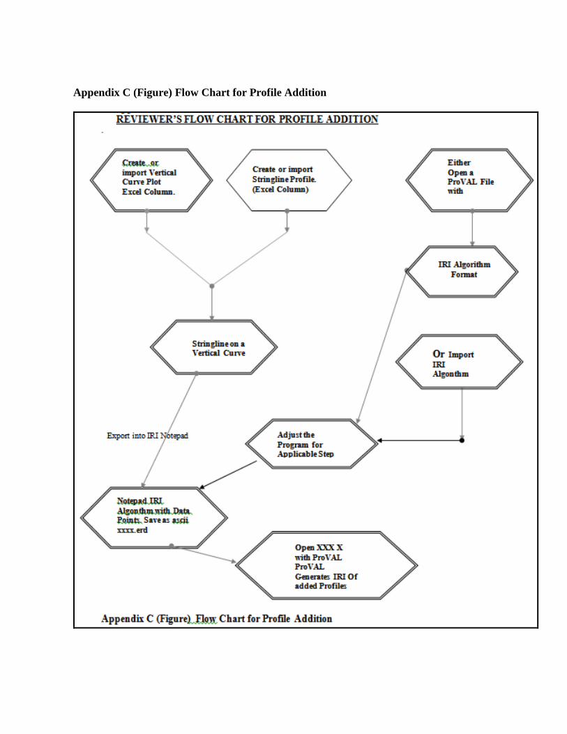
Appendix C (Figure) Flow Chart for Profile Addition