Embed Size (px)
Citation preview

ANALYZING CONSUMER WILLINGNESS TO PAY FOR A PECAN SNACK PRODUCT
by
KATY SWICKARD
(Under the Direction of John McKissick)
ABSTRACT
Demand for pecans has been stagnant over that last seven years, leading pecan producers
to look for new ways of increasing demand. With new storage techniques it may be possible to
produce snack products of pecans similar to that of peanuts. A national survey of 913 people was
performed in order to obtain data on the demographics and buying habits of pecans consumers. A
Tobit model was used to analyze the survey data to determine the mean Willingness to Pay for a
pecan snack product. The mean willingness to pay was estimated to be $0.89 for a snack size
bag of pecans. In addition, the average pecan consumer does not purchase pecans very often,
fewer than three times a year, with most purchasing one pound bags of halves. Almost eight
percent of pecan consumers surveyed indicated that they had had a problem with rancidity in
pecans.
INDEX WORDS: Pecans, Willingness to Pay, Demand, Snacks, Contingent Valuation,
Consumer Survey

ANALYZING CONSUMER WILLINGNESS TO PAY FOR A PECAN SNACK PRODUCT
by
KATY SWICKARD
B.S., Purdue University, 2002
A Thesis Submitted to the Graduate Faculty of The University of Georgia in Partial Fulfillment
of the Requirements for the Degree
MASTER OF SCIENCE
ATHENS, GEORGIA
2005

© 2005
Katy Swickard
All Rights Reserved

ANALYZING CONSUMER WILLINGNESS TO PAY FOR A SNACK PECAN PRODCUT
by
KATY SWICKARD
Major Professor: John McKissick
Committee: Chung Huang Jim Daniels
Electronic Version Approved: Maureen Grasso Dean of the Graduate School The University of Georgia August 2005

iv
ACKNOWLEDGEMENTS
First, I would like to thank my parents for having faith and full support of my decision to
leave behind a home that I knew and loved to a place that was new and unfamiliar. To my mom,
thank you for your love and encouragement to always do what is right for me in terms of my
education, my life, and my happiness. I am deeply thankful for all you have done for me these
past two years while I have been so far from home. I am not sure my time at UGA would have
gone as smoothly if you had not always stayed positive and excited about everything I
participated in. To my dad, thank you for all of your encouragement and love. Thank you for
moving me back and forth across the middle United States.
I am truly grateful to Dr. McKissick for providing me with the assistantship to work with
the Center for Agribusiness and Economic Development while I attended graduate school. Dr.
McKissick, thank you for the opportunity to work with you on several projects that allowed me
to gain experience and a sense of accomplishment. I have enjoyed getting to know all the people
who make up the Center and appreciate all those who have assisted me in some way or another.
Next, I would like to thank Dr. Huang for the hours upon hours he spent with me going
over my model and assisting me with the numerous errors that crept up. Without him I am not
sure if my thesis would even be ready as a rough draft. Dr. Huang has an endless amount of
patience and I appreciate him not putting up a sign and banning me from his office which I
visited more than once a day the last few months!
I would like to thank Dr. Daniels for his assistance and enthusiasm for this project. He
has been extremely helpful in providing me with contacts and pecan samples when I needed
them.

v
The next two people I would like to thank have made the biggest difference in my time
during graduate school; I only wish I had met them earlier. Dr. Kent Wolfe, thank you for all of
your encouragement and remaining optimistic during my time here. You are always smiling and
cheerful and it makes all of those around you smile. Thank you for the opportunity to have the
presentation experience during the Agritourism workshops.
Dr. Michael Best, I could write an entire chapter for you and still not be able to convey
just how much you have helped me and mean to me as a teacher, co-worker, and a friend. You
are almost the single reason I am actually finishing, but I cannot give you that much credit! Just
like Dr. Wolfe, you are always smiling and cheerful about something (usually some 1980’s song
you heard on the radio and cannot figure out who sang it). You have pushed me and at the same
time let me on my own. You have read my thesis probably ten times and have provided me with
suggestions and corrections in order to finish on time (for the second time). No one else here
would have spent as much time with me and my thesis as you have. Thank you for keeping my
spirits up when I become frustrated and overwhelmed. Again, I can babble on and on about how
much you have done for me, but to keep it simple, Thank You.
Last but not least I want to thank all of my grad school buddies I have made here.
Without your support during classes and in general I would still be figuring out how to calculate
Beta hat and flipping through the SAS manual looking for the code for a Do Loop. At least I can
now say I have skills and not just those like bow-staff and num-chuck skills, but real skills like
navigating the Loop, figuring out which Mexican restaurant makes you the least ill, and on game
day you either get there early or you don’t get there at all.
vi
TABLE OF CONTENTS
Page
ACKNOWLEDGEMENTS........................................................................................................... iv
LIST OF TABLES....................................................................................................................... viii
LIST OF FIGURES .........................................................................................................................x
CHAPTER
1 INTRODCUTION .........................................................................................................1
Pecan Production Overview ......................................................................................1
Pecan Market Structure .............................................................................................4
Pecan Import and Export Markets.............................................................................7
Pecan Prices.............................................................................................................10
Pecan Consumption.................................................................................................12
Storing Pecans .........................................................................................................14
Problem Statement ..................................................................................................15
2 LITERATURE REVIEW ............................................................................................17
Contingent Valuation Method and Willingness to Pay ...........................................17
CVM and WTP for Organic, Eco-Labeled, and Country-of-Origin Products ........22
Value Added Produce..............................................................................................25
3 THEORETICAL FRAMEWORK...............................................................................29
Measuring the Economic Value of a Product..........................................................29
Utility and Demand .................................................................................................29

vii
Willingness to Pay...................................................................................................33
Utilizing Contingent Valuation to Determine WTP................................................38
4 Data Collection and Results.........................................................................................41
Survey Design .........................................................................................................42
U.S. and Survey Respondent Characteristics ..........................................................51
Survey Respondent Characteristics of Pecan Snack Consumers ............................53
Additional Demographic Characteristics Analysis .................................................57
Survey Results to Selected Pecan Consumer Questions .........................................63
5 Empirical Results and Analysis ...................................................................................66
Overview of Tobit Model........................................................................................66
Model Results..........................................................................................................70
6 Summary and Conclusions ..........................................................................................78
Conclusions .............................................................................................................78
Limitations and Future Research.............................................................................82
REFERENCES ..............................................................................................................................84
APPENDICES ...............................................................................................................................89
A Consumer Pecan Use Survey 2004..............................................................................89
B Homoscedastic and Heteroscedastic Tobit Model Comparison ................................115
viii
LIST OF TABLES
Page
Table 1.1: Fatty Acid Content of Pecan Oil...................................................................................12
Table 4.1: Reasons for Not Purchasing Pecans in the Past 24 Months and Percentages...............44
Table 4.2 Definition and Summary of Sample Characteristics .....................................................45
Table 4.3: Consumer Pecan Perceptions........................................................................................47
Table 4.4: Descriptive Statistics of Answers to WTP Question ....................................................51
Table 4.5: Frequency of Purchasing Pecans as a Snack ................................................................55
Table 4.6: Places Pecan are Purchased the Most by Region..........................................................57
Table 4.7: WTP for Each Income Level ........................................................................................57
Table 4.8: WTP for Each Region...................................................................................................58
Table 4.9: Mean WTP by Income Levels and Region...................................................................58
Table 4.10: Mean WTP by Region and Where Pecans are Most Often Purchased .......................59
Table 4.11: Mean WTP by Income Level and Where Pecans are Most Often Purchased ............59
Table 4.12: Mean WTP by Income Level and the Size of Bag that Pecans are Most Often
Purchased.......................................................................................................................60
Table 4.13: Percent Likely to Purchase a Raw Pecan Snack by Region .......................................60
Table 4.14: Percent Likely to Purchase a Sugar and Spice Pecan Snack by Region.....................61
Table 4.15: Percent Likely to Purchase a Roasted Pecan Snack by Region..................................61
Table 4.16: Percent Likely to Purchase a Flavored Pecan Snack by Region ................................62
Table 4.17: Percent Likely to Purchase a Salted Pecan Snack by Region.....................................62
ix
Table 4.18: Percent Likely to Purchase a Spicy Pecan Snack by Region......................................63
Table 4.19: Percent Likely to Purchase a Glazed Pecan Snack by Region ...................................63
Table 5.1: Variable Descriptions for Tobit Model.........................................................................71
Table 5.2: Regression Results for the Tobit Model for a Single Serving Snack Size Bag of
Pecans............................................................................................................................74
Table 5.3: Estimated Elasticities of the Heteroscedastic Tobit Model .........................................77

x
LIST OF FIGURES
Page
Figure 1.1: Map f the United States and Mexican Pecan Producing States.....................................3
Figure 1.2: Total United States Utilized Pecan Production .............................................................5
Figure 1.3: Total Value of Pecan Production in $1,000 ..................................................................8
Figure 1.4: Total United States Pecan Supply .................................................................................9
Figure 1.5: United States Pecan Imports and Exports ...................................................................11
Figure 1.6: Pecan, Walnut, and Almond Consumption from 1980-2002 ......................................13
Figure 3.1: Maximum Utility Level Derived by Indifference Curves and Budge Constraints......31
Figure 3.2: Linear “smooth” Demand Curve.................................................................................32
Figure 3.3: Consumer Surplus: Area “A” .....................................................................................34
Figure 3.4: Utility Maximization for WTP....................................................................................37
Figure 3.5:Expected Consumer Surplus from Dichotomous Choice.............................................40
1
Chapter 1
Introduction
The pecan, Carya illinoinensis is the only native tree-nut grown for commercial
production in the United States. According to historians, the word pecan is of Algonquin origin
used to describe any “nut requiring a stone to crack” (Taylor, 2001). It is indigenous to the
Southwestern United States and Mexico, and grows up along the Mississippi River into Indiana
and Illinois. The pecan served as a staple of the Native Americans diet long before the
Europeans arrived. Later, pecans were traded for furs and tobacco (Rosengarten, 1984).
The pecan is a nutritional and tasty nut that appeals to a wide array of people. The
desirable flavor, texture and appearance make pecans attractive as an ingredient in baked goods,
candies, confections, snacks, salad toppings, ice cream, and various meat and vegetable dishes.
The flavor of the pecan is compatible with most foods as they are often eaten sugared, spiced or
raw. The pecan’s texture allows it to be used in halves or pieces (Hubbard et al., 1987). A study
by Park and Florkowski (1999) determined that consumers identified pecans as premium nuts
along with almonds, pistachios, and macadamias.
Pecan Production Overview
Pecans are perennial in growth and production; they begin to bear nuts normally in ten to
twelve years. Pecan trees have an alternate bearing pattern meaning one year a tree will have a
heavy crop while the next year will be lighter. There are two general types of pecans:
native/seedling and improved varieties. The natives and seedlings are harvested from trees that

2
are wild and have not been genetically altered. These generally do not have any variety name.
Improved varieties are produced on trees that have been grafted or budded. In general, improved
varieties produce a more consistent crop with a more desirable quality such as size of kernel and
color. According to Hubbard et al. (1987), Georgia has an initial comparative advantage in the
pecan industry. The orchards are established, producing, and being expanded and renewed.
Growers have been replacing old, traditional varieties with new improved varieties. The newer
varieties are of better quality and better suited for the gift trade industry (Hubbard et al., 1987).
In the southeast more than 80 percent of pecan production comes from improved varieties.
About 37 percent of Georgia pecans are of the new variety (Hall et al., 1998).
Large scale production began in the late 1880’s on the Mississippi Delta and in the early
1900’s; hundreds of thousands of acres were planted in the southeastern states, mostly of Stuart
variety (Taylor, 2001). Production areas in the U.S. are defined into two categories: the
Southeastern area includes Georgia, Alabama, Florida, Mississippi, North Carolina, South
Carolina; and the Southwestern area includes Texas, New Mexico, Arizona, Oklahoma,
Louisiana, Arkansas, and California (Hubbard et al., 1987). Texas accounts for one-third of the
U.S. pecan farms (with almost twice as many trees as Georgia), however Georgia has the greatest
output (USDA, May 2003). The United States produces about 75 percent of the total world
supply of pecans followed by Mexico producing about 20 percent (Johnson, 1998). Figure 1.1 on
page 3 is a map of the United States and Mexican pecan producing states. In addition to Mexico,
pecans are also grown in Australia, Brazil, South Africa, Israel, and a few other countries in
limited quantities.

3
Figure 1.1 Map of the United States and Mexican Pecan Producing States
4
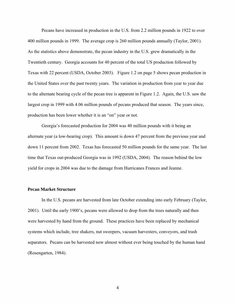
Pecans have increased in production in the U.S. from 2.2 million pounds in 1922 to over
400 million pounds in 1999. The average crop is 260 million pounds annually (Taylor, 2001).
As the statistics above demonstrate, the pecan industry in the U.S. grew dramatically in the
Twentieth century. Georgia accounts for 40 percent of the total US production followed by
Texas with 22 percent (USDA, October 2003). Figure 1.2 on page 5 shows pecan production in
the United States over the past twenty years. The variation in production from year to year due
to the alternate bearing cycle of the pecan tree is apparent in Figure 1.2. Again, the U.S. saw the
largest crop in 1999 with 4.06 million pounds of pecans produced that season. The years since,
production has been lower whether it is an “on” year or not.
Georgia’s forecasted production for 2004 was 40 million pounds with it being an
alternate year (a low-bearing crop). This amount is down 47 percent from the previous year and
down 11 percent from 2002. Texas has forecasted 50 million pounds for the same year. The last
time that Texas out-produced Georgia was in 1992 (USDA, 2004). The reason behind the low
yield for crops in 2004 was due to the damage from Hurricanes Frances and Jeanne.
Pecan Market Structure
In the U.S. pecans are harvested from late October extending into early February (Taylor,
2001). Until the early 1900’s, pecans were allowed to drop from the trees naturally and then
were harvested by hand from the ground. These practices have been replaced by mechanical
systems which include, tree shakers, nut sweepers, vacuum harvesters, conveyors, and trash
separators. Pecans can be harvested now almost without ever being touched by the human hand
(Rosengarten, 1984).

5
Figure 1.2 Total United States Utilized Pecan Production
Source: USDA, 2004
0
50,0
00
100,
000
150,
000
200,
000
250,
000
300,
000
350,
000
400,
000
450,
000
1980
1982
1984
1986
1988
1990
1992
1994
1996
1998
20
0020
02
Seas
on
1,000 pounds
1,00
0 lb
s

6
Once harvested the moisture content must be reduced in order to obtain higher quality
pecan products. The pecans are taken to shellers or sold to accumulators or buyers who then sell
to shellers or wholesalers. Wholesalers, normally resell to retail or industrial outlets, while
shellers are responsible for separating the nutmeat from the shell. After pecans have been
shelled, the nut meat is sized, graded, and packaged. Quality is determined by the percentage of
kernel in shell (amount of nut meat), color (lighter brown being most desired), shell thickness,
and oil content. Improved varieties tend to have more favorable attributes (USDA, May 2003).
(Lillywhite et al., 2003). The size of packages most commonly used for pecan halves and pieces
is either smaller packages of 2 to 12 ounces or 30 pound boxes.
The smaller packages are sold to retail outlets and wholesale distributors, while the larger
boxes are sold to processing companies such as confectioners, bakers, and ice cream
manufacturers (Lillywhite et al., 2003). Bakeries and confectioners are the largest users of
shelled pecans with the lesser quantities going to retailers, ice cream manufacturers, and
wholesalers. Pecans for processing compete with other tree nuts such as almonds, walnuts,
filberts, and hazelnuts. Peanuts do not directly compete with pecans since they are not in the
same price range. Peanuts are usually found in candies and salted mixes, while tree nuts
dominate the bakery and ice cream products (Lillywhite et al., 2003). In recent years there has
also been an increase in demand for pecans due to the gift trade and school fundraisers.
Neither the state nor the federal governments have any influence on the supply or price of
pecans. This makes the industry a competitive-free market (Wood, 2000). At the farm level,
pecans contributed over $275 million dollars to the U.S. economy. The highest valued crop on
record was during the 1999/2000 season at $330 million. This particular season also had the
highest production yield on record. In Georgia, pecans contribute significantly to the economy.

7
In 2003, pecans contributed $69 million in total farm value to the economy as seen in Figure 1.3
on page 8. The farm value of pecans tends to follow a similar pattern to that of total farm
production in the sense that there is a distinction between alternate bearing years of the pecan
tree. Higher production volume correlates to higher value of production.
Pecan Import and Export Markets
About two-thirds of the United States total tree-nut production is exported with the quantity
of pecans exported being less than 20 percent of U.S. production. Pecan exports increased eight
percent from 1980-1990 and have been steadily increasing since 1990. The U.S. exports a
significant amount of pecans to Canada, Mexico, and Europe (Johnson, 1998). Pecan markets in
China have been growing quickly since 2001. In-shell exports were almost non-existent until
2000 and since 2003 China has become the second largest export market for U.S pecans (USDA,
May 2003). The pecan trade relationship between the United States and Mexico is considered
complementary in that exports to Mexico have increased while imports to the U.S. have
increased as well (Peña et al., 2001). It is believed that the higher quality pecans produced in
Mexico are exported to the U.S. to supplement for low production years and lower quality
pecans.
Imports from Mexico boost total supply and stock levels. Imports are about one quarter the
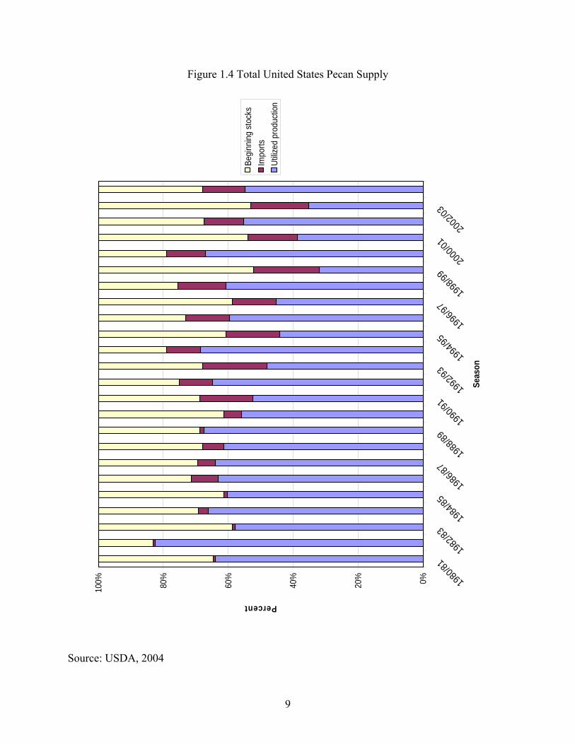
size of the U.S. crop. Figure 1.4 on page 9 illustrates how significant pecan imports have
become as a part of total U.S. pecan supply. The supply of pecans (production + imports +
beginning stocks) has outpaced use or demand (domestic consumption + exports), which has
gradually increased stock levels during the recent years (Johnson, 1998).

8
Figure 1.3 Total U.S. Value of Pecan Production in $1,000
Source: USDA, 2004
0
50,0
00
100,
000
150,
000
200,
000
250,
000
300,
000
350,
000 19
8019
8119
8219
8319
8419
8519
8619
8719
8819
8919
9019
9119
9219
9319
9419
9519
9619
97 19
98 19
9920
0020
0120
0220
03
Seas
on
Dollars ($1,000)
Valu
eG
eorg
ia
9
Figure 1.4 Total United States Pecan Supply
Source: USDA, 2004
0%20%
40%
60%
80%
100% 198
0/81 198
2/83 198
4/85 198
6/87 198
8/89 199
0/91 199
2/93 199
4/95 199
6/97 199
8/99 200
0/01 200
2/03
Seas
on
Percent
Begi
nnin
g st
ocks
Impo
rtsUt
ilized
pro
duct
ion
10
The cyclical nature of the pecan industry can easily be seen in Figure 1.4. Also, beginning
stocks are usually greater following a high production year due to the larger amounts of pecans
being stored.
Imports are greater during low production years and lower during higher production years.
As seen in Figure 1.5 on page 11 the U.S. has become a net importer of pecans. The balance of
trade turned negative as imports began to exceed exports during the 1980’s and since the 1990’s
imports have comprised a large percentage of total U.S. supply. In the mid-1980’s in-shell pecan
imports increased 37 percent which was around the same time that exports began to increase.
After the North America Free Trade Agreement (NAFTA) was implemented in 1994,
imports increased 50 percent. Shelled imports in the U.S. expanded roughly 350 percent before
NAFTA in the mid-1980’s, but only 31 percent afterward (Peña, 2001). Figure 1.4 shows U.S.
total pecan exports and imports over a period of twenty years.
Pecan Prices
Statistically, pecan supply explains only a part of the variation in prices from year to
year. Pecan growers must sell their crop in a short time period where there are relatively few
buyers. There are other economic factors that influence prices such as the size of the Mexican
crop, current availability of improved versus native pecans, stocks, and supplies and prices of
competitive tree-nuts (Johnson, 1998). In addition to the above factors, pecan crop quality can
also be a determinant in prices.
Throughout the 1990’s, pecan prices grew at an average annual rate of 12 percent
(USDA, May 2003). Since 1990, pecan grower prices on a per-pound shelled basis have been
higher than the same for almonds, walnuts and hazelnuts.

11
Figure 1.5 United States Pecan Imports and Exports
Source: USDA, 2004
0
5,00
0
10,0
00
15,0
00
20,0
00
25,0
00
30,0
00
35,0
00
40,0
00
45,0
00
1980
/81 19
82/83
1984
/85 19
86/87
1988
/89 19
90/91
1992
/93 19
94/95
19
96/97
1998
/99
2000
/01 20
02/03
Seas
on
Pounds
Impo
rts
Expo
rts

12
Pecan Consumption
Pecans account for 25 percent of total nut tree-nut consumption on a per pound basis.
This places them directly after almonds and walnuts in terms of consumption. Since the 1980’s,
pecan consumption has been stagnant and has actually trended downward since 1998. The
average annual pecan consumption in the U.S. over the past five years was approximately 0.42
pounds. This is a slight decrease from previous year’s averages. Walnut consumption is closer
to that of pecans with 0.47 pounds per capita consumed annually (USDA, 2004).
As seen in Figure 1.6 on the following page, consumption patterns have been similar for pecans
and walnuts from 1980 until recently. In the past generally, more pecans were consumed than
walnuts. However, since 2002 walnuts have outpaced pecans. The consumption of almonds has
also increased rapidly the past fifteen years compared to pecans and walnuts. The reasons
behind this phenomenon may include crop size, consumer attitudes and preferences towards
certain nuts, and the industries’ marketing strategies.
In recent years, the consumption trend for “heart-healthy fats” has increased. Pecans
contain nearly 65 percent monounsaturated and 28 percent polyunsaturated fats; these are
considered good fats (Taylor, 2001). Table 1.1 below presents the breakdown of fat content of
pecans.
Table 1.1 Fatty Acid Content of Pecan Oil Fatty Acid % Type Palmitic 5 Saturated Stearic 2 Saturated Oleic 65 Monounsaturated Linoleic 26 Polyunsaturated Linolenic 2 Polyunsaturated Source: Pecan Storage, Wagner 1980

13
Figure 1.6 Pecan, Almond, and Walnut Consumption from 1980-2002
Source: USDA, 2004
0.00
0.20
0.40
0.60
0.80
1.00
1.20 19
80/81
1982
/83 19
84/85
1986
/87 19
88/89
1990
/91 19
92/93
1994
/95
1996
/97 19
98/99
20
00/01
2002
/03
Seas
on
Per Capita Consumption
Alm
onds
Wal
nuts
Peca
n
14
Consumers are encouraged to eat foods with these types of fats in place of those high in
saturated fats. The FDA recently approved a claim regarding pecans and other nuts in their roles
in reducing heart disease (ilovepecans.org, 2003). Many tree nut industries have begun to use
these healthy claims in their marketing designs. The pecan industry could benefit from labels or
other such marketing techniques involving this approach to increase pecan consumption.
Storing Pecans
Pecans are semi-perishable, and unless stored properly may become inedible due to
rancidity, mold, and insects. It has been shown that adequate drying, packaging, and
refrigeration are the most important facts in preserving the quality of a shelled pecan. Proper
storage is one of the solutions to the problem of carryover of pecans from heavy crops to lighter
crops the next year (Woodruff, 1979).
Experiments conducted by the Georgia Experiment Station have shown that controlled
refrigerated storage can retard rancidity while preserving the natural color, flavor, and texture.
High moisture in nuts is the most significant cause of deterioration during pecan storage and it
can cause a nut to become inedible within two weeks.
Research has established that storage life of pecans can be extended by the addition of
antioxidants. In the early 1970’s BHA, BHT, and propyl gallate were being used to treat nuts. It
was determined that nut meats treated with TenoxBHA and TenoxBHT used in baked goods had
about twice the shelf life as untreated nuts (Woodruff, 1979). Research has also shown that
shelled pecans stored in vacuum pack bags keep longer than those kept in boxes alone. Pecans in
vacuum-packed bags stored at 32˚F can last for two to three years.
15
Problem Statement
Georgia pecan farmers have experienced highly variable prices and profits. Pecan
producers are examining new ways to market pecans and thus increase pecan consumer demand,
leading to higher farmer prices. The shelf life of pecans is viewed as a problem in the pecan
processing industry. Consumers tend to purchase pecans seasonally, thus making long-term
storage an important issue for Georgia pecan growers. While most other snack nut products are
shelf-stable, pecans on the other hand tend to become rancid and bitter in a relatively short
period of time due to their high oil content. For this reason, pecans are kept in cold storage until
used by the processor.
New technologies are being developed that may give the pecan industry the potential to
develop a shelf-stable pecan snack product. One such technology currently being researched is
the use of supercritical carbon dioxide which infuses pecans with an antioxidant in order to
extend the shelf-life and retard rancidity development. An important research question is
whether or not consumers are willing to purchase products treated to extend shelf-life. Such a
question would have to be answered before producers invest the capital required for this new
technology.
In addition to researching the potential demand for new extended shelf-life products, it is
also important for policy makers and pecan industry leaders to understand the factors affecting
domestic consumption of pecans. This should help determine how the low consumption trend of
the industry could be reversed. For example, the pecan has been an important product during the
winter holiday season of November and December. Producers would like to adjust these
consumption patterns to expand purchases throughout the market year. In order for this to occur,
the reasons why consumers do not purchase pecans throughout the year must be elucidated. In

16
addition, why consumers’ use pecan, what form do they purchase pecans, prices paid, and
consumer profiles may help determine the best way to capture more of the tree nut market. A
national survey of consumers could clarify the importance of these factors.
The major objective of this study is to determine the likelihood of consumer’s willingness
to purchase and how much they are willing to pay for a new single service size pecan snack
product using socio-demographic and attitudinal characteristics. In addition, the study will
evaluate consumers purchasing and consumption practices in regard to the pecan as a snack nut.
This would include their knowledge and uses of pecans.
Specific Objectives are:
1. Determine current consumer uses, and attitudes/perceptions of pecans
2. Determine the demographic profile of potential pecan snack consumer
3. Determine the willingness-to-pay and willingness-to-purchase of a 2.5 ounce single-
serving snack size bag of pecans

17
Chapter 2
Literature Review
Contingent Valuation Method (CVM) has become a useful tool in determining
willingness to pay (WTP) over the past fifteen years. Dasgupta et al. (2000), Loueiro and
Umberger (2002), Blend and van Ravenswaay (1999), Misra et al. (1991), Govindasamy and
Italia (1998), Wessells and Anderson (1995) among others, have performed research in this area.
Recently, WTP and CV have been used to research demand for safer meat products, eco-labeled
foods, and organic products. However, there have been few WTP studies for new, hypothetical
products, and none in the tree nut industry. Most manufactured food companies that provide and
market snack products, including tree nut products, normally conduct field tests to get an idea of
what consumers will pay for a product. In these tests, companies will produce a new item and
choose an area to market the item. By selling the product at different prices and quantities, the
company will be able to analyze the product’s acceptance level and the demand. This chapter
will highlight studies that have utilized the CVM to identify consumer’s WTP for products or
estimate the products value to consumers.
Contingent Valuation Method and Willingness to Pay
Researchers generally find the contingent valuation method the most appropriate for
measuring the value of non-market goods. The CVM is more flexible and has a relatively low
cost compared to other methods such as experimental markets. Questions have been raised about
direct methods such as the CVM, dichotomous choice questioning and experimental markets
reliability as the best methods in determining a mean willingness to pay.
18
One issue is that consumers may not have enough information about the risks and
therefore may give an inaccurate monetary evaluation from risk avoidance. Another problem is
the extension of WTP results to other foods. Within the CVM, most of the analyses are
hypothetical situations in which the consumer may take less seriously than a real one and
therefore tend to overestimate or underestimate their true WTP. This creates unwanted bias
which affects the true mean WTP for a product (Hanemann, 1991).
Researchers have used a variety of models over the years to analyze the WTP and
determine the level of WTP. For example, a study that was conducted by Rimal and Fletcher
(2002) focused on measuring the impacts of nutritional consideration indices and household
socioeconomic characteristics on market participation and purchase levels of snack peanuts. The
authors used data from a household peanut purchasing survey conducted by Gallup in 1997 and
three models were evaluated to test the relationship between nutritional awareness and demand
for a commodity. Snack peanuts account for twenty-five percent of the domestic edible peanut
use. The market share of snack peanuts in the U.S. snack food industry had been declining over
the past several years.
According to Rimal and Fletcher (2002), Cragg’s double hurdle model is more general,
though a consumer must pass two obstacles before determining a positive level of consumption
of peanuts. The consumer must be a potential consumer of snack peanuts and consume some of
the product. They found that this so called “double hurdle” model provided the best
representation of consumer’s purchase level decisions of snack peanuts. The Tobit and
Complete Dominance models underestimated the impact of the explanatory variables on
household’s decision to purchase snack peanuts. Household Income was found to be one the
most important factors in participation and frequency of purchases in the double hurdle model.

19
The variable Race also had an effect on frequency of snack peanut purchases. Nutritional
considerations were found not significant on the decision to participate in the peanuts; however,
they were significant in making purchasing decisions. Residence and gender were insignificant
factors in market participation, though significant for purchasing frequency. Number of children
in a household had a negative effect on the decision of how often the household would purchase
snack peanuts. The authors concluded that peanut producers should separate their products from
the general snack category. In other words, it seems that labeling peanuts as a snack has a
negative effect on purchasing habits. Producers need to expand on the positive nutritional
attributes of peanut products.
Huang (1993) developed a theoretical model to analyze consumer risk perceptions,
attitudes, and behavior intentions regarding pesticide use on agricultural commodities. The
model is a three-equation simultaneous framework in which the three dependent variables are
based on data collected from a Georgia consumer survey. The first variable, consumers’ risk
perception toward the use of pesticide in fresh produce (RP) was constructed from a binary scale.
The second variable ATTI, which defines a consumer’s attitude toward regulatory actions on the
use of pesticides, was also binary. For the last variable, the willingness to pay (WTP) was
measured using a scale from one to five for willing or not willing to pay a higher price for
certified residue free (CRF) produce.
At first each equation was estimated by regressing each dependent variable on all
independent variables. The reduced forms of RP and ATTI were then estimated by the
maximum likelihood Probit model. Ordinary least squares (OLS) was used for the reduced WTP
equation. When estimating the third equation, both RP and ATTI are independent variables used
to evaluate the WTP. Fitted values were then found for each of the dependent variables giving
20
way to new terms RPhat, ATTIhat, WTPhat . In the second stage, the maximum likelihood Probit
and OLS was used to estimate the structural parameters for the fitted terms.
Huang’s (1993) results indicate that attitude was linked to perception and willingness to
pay which then affects consumers’ attitudes toward pesticide use. The study suggests that those
who have used or have knowledge of chemical pesticides for home gardening were less likely to
be worried about the use of pesticides on fresh produce. Another finding was those consumers
who wanted fresh produce tested for residues were willing to pay another three percent than
those who did not.
Huang (1993) found most of the socioeconomic and demographic variables were
statistically significant. Married females with one or more children and are employed have more
concern about the use of pesticides. Income was also found to be a statistically significant
predictor of willingness to pay for certified free of pesticide produce. The negative signs found
on education and household size indicate that respondents with larger families and higher
education are less likely to pay a premium for CRF produce. This may be due to the fact that
they believe the benefits of pesticide use offset potential risks. Huang (1993) suggested that
consumers need more education about nutrition and food safety risks which would help reduce
misinformation and aid in the understanding of health risks carried by some foods.
Mukhopadhaya et al. (2004) estimated consumers’ willingness to pay for a hypothetical
vaccine that would deliver a 1-year, 5-years, and 10-years, or lifetime protection against
Salomenella, E. coli, or Listeria. The contingent valuation method was used to estimate the WTP
that would protect a person from the major food borne pathogens. A survey was conducted and a
dichotomous choice question was used to elicit the WTP. The yes or no responses are translated

21
into mean or median WTP. A Tobit model was used to estimate the dollar amounts that
consumers were willing to pay for the duration of protection.
Respondents were randomly selected for the telephone survey and the bid amounts were
randomly assigned to those respondents. The analysis included some important socioeconomic
variables such as age, income, education, home setting, and current health conditions. The
researchers used a number of dummy variables to indicate if a respondent was a member of a
certain group or not. The empirical analyses were performed using the dollar values for the
willingness to pay as the dependent variable. The results from the Tobit model indicate that
consumers were willing to pay for protection against food borne pathogens. They are willing to
pay more for longer protection time. It was also found that the respondents would pay more for
protection against E. coli compared to the other two diseases. Decision makers can use WTP
studies such as this to set policy that affects both consumers and producers.
Dasgupta et al. (2000) used a Probit model to analyze the results of a telephone survey of
consumers conducted to determine preferences for trout steak and the feasibility of such a
product. At the time the study was conducted, the trout industry had been losing market share.
The survey was used to extract consumer attitudes and purchasing behaviors toward various
seafood and meat products. Trout steaks were the main focus of the survey. The survey was
also intended to extract consumers’ willingness to purchase fresh or frozen trout steaks. They
found that consumers were more receptive to fresh trout steaks than frozen steaks. The
researchers used an ordered Probit regression analysis that identified consumer attributes that
affected their willingness to purchase the trout steaks, fresh or frozen. In this study, ethnicity,
education, income, household size and price perception significantly affected trout-steak
purchasing decisions. The chief implication is the preference of fresh trout steaks by Hispanics,
22
consumers with a large household size, and those who consider trout to be more expensive than
other meats. These results were intended to help the trout industry determine how to market
fresh and frozen trout steaks.
CVM and WTP for Organic, Eco-labeled, and Country-of-Origin Products
There has been a plethora of studies on improved food-safety and labeling of foods.
Most are due to increasing consumer concerns of pesticide use, safety issues, and disease-free
meats.
Loueiro et al. (2002) conducted a WTP and socioeconomic study for Eco-labeled apples.
The objectives of this study were to analyze the impact of factors influencing consumers’ WTP
for eco-labeled apples and estimate a mean WTP for the eco-labeled apples. They surveyed
consumers in grocery store locations where there was a variety of produce offered. From the
survey they obtained information of the consumers’ attitudes about the environment and food
safety, knowledge and perceptions of eco-labels and socio-demographic information. To
estimate the mean WTP, Loueiro et al. (2002) used a double-bounded Logit model because it had
been shown as it was more efficient than a single-bounded model. The researchers conclude that
consumers are willing to pay a small percentage (about 5 percent) above the base price for eco-
labeled apples. They also conclude that the important significant variables were children under
18 years old and being female. In a similar study, Blend and van Ravenswaay (1999) conducted
a telephone survey to determine the consumer demand for eco-labeled apples. The survey was
conducted giving respondents different scenarios with and without eco-labeling. Open-ended
questions were used to determine quantities of eco-labeled apples one would purchase. They
used both a Cragg double hurdle model and Tobit model to estimate demand. They determined

23
over half of the respondents would be willing to purchase eco-labeled apples. As the price
premium increases, the probability of purchasing the eco-labeled apples decreases. Even with a
premium of $0.40, over 40 percent of respondents were still willing to try these apples.
A survey conducted by Misra et al. (1991) allowed them to gather data to determine
consumers’ willingness to pay for fresh produce that is certified as free of pesticide residues. It
had been noted previously that perceptions among Americans about pesticide residue were high
and induced some private markets to do some testing on labeling programs. Questions were
asked on the consumer survey to elicit consumers’ perceptions, attitudes, and concern towards
the use of pesticides in the production of fruit and vegetables. For the willingness to pay section,
consumers were asked if they would pay a higher price for fresh produce that had been certified
as residue-free. If they answered yes, then they were then asked how much more they would pay
with five percent increments. Misra et al. (1991) used the Probit model to estimate the
probabilities of the consumers’ willingness to pay. The results suggested that consumers were
generally not likely to pay a premium for produce certified as free of residues. Most variables
were significant at the 0.1 level. Concern expressed about pesticides, the importance of testing
for pesticide, age and income were all significant variables. The negative sign on income may
imply that consumers in lower income groups will be less likely to pay a premium than
consumers in higher groups. More than half of the respondents either refused to pay a higher
price or were not sure. One factor they noted was that consumers may reason that food safety is
a public good and therefore the government should have a role in ensuring that produce is free of
pesticide residue.
Govindasamy and Italia (1998) estimate consumers’ willingness to purchase integrated
pest management (IPM) labeled produce. IPM is pest control system developed to tackle

24
problems with pests that build immunity to chemical pesticides. It is more cost-effective than
organic production and potentially safer than other agricultural processes. Through the survey,
they found that consumers were receptive to the IPM produce. Two Logit models were used to
determine the effects of sociodemographic factors that influence the willingness to purchase
conventional and IPM grown produce. They chose the Logit model because its “asymptotically
characteristic constrains the predicted probabilities to a range of zero to one” (Govindasamy and
Italia, 1998). The results show that consumers would be willing to purchase IPM labeled
produce and many would be willing to switch grocery stores to purchase IPM produce. Using a
label with IPM could help growers differentiate and add value to their products. Direct market
establishments such as roadside stands and farmers’ markets would work well to introduce IPM
labeled produce. Income, age, suburban or rural locations, and those who have previous
knowledge of IPM affect purchasing decisions. The willingness to purchase IPM produce
increase with Income and decreases with Age with the opposite results for conventionally
produced goods. Educating consumers of IPM produce will increase acceptance and demand.
The results from this study were quite positive, especially for producers interested in IPM
systems on their farms.
Country-of-origin labeling is a method to allow consumers to identify where the foods
that they purchase are produced. Loureiro and Umberger (2002) performed an analysis of
consumers’ preferences and the economic effect of country of origin labels on beef. They also
calculated premiums for U.S. labeled beef versus imported beef. Consumers in grocery stores
were selected randomly to participate in the survey which elicited purchasing behavior, desirable
beef qualities, food safety attitudes, WTP for a tax program to support mandatory country-of-
origin labels and WTP for a U.S. labeled steak and hamburger. For the analysis of the survey

25
they used independent Logit models. WTP estimates were calculated using the “grand constant”
formula (see Giraud et al., 1999). Confidence intervals were constructed using a bootstrapping
technique. Loureiro and Umberger’s (2002) results show that consumers are concerned about
food-safety issues and are willing to pay a premium for the mandatory country-of-origin labeling
program. Also, consumers are willing to pay a premium for U.S. labeled steaks and hamburger.
Education, food safety attitudes, number of children in household, and gender were all
significant variables.
Wessells et al. (1999) created a survey for participants to compare seafood products that
were certified with an eco-label and those without any certification. The Logit model was
applied to the collected data. Results indicate that preferences for eco-labeled fish will differ
across regions and consumer groups. One significant variable is the premium paid for certified
products. The results of this study indicated that as the premiums paid for certified products
increased, consumers are less likely to choose certified products. In general, consumer
preferences affected the probability of choosing certified seafood products. Respondents who
tend to purchase frozen seafood are less likely to choose a certified product. Eco-labels will only
be applicable to those who purchase seafood. Lastly, consumer education about fish stocks will
need to take place in order to have a successful certification program.
Value-Added Produce
Other studies have focused on the demand for domestically labeled products as well as
locally grown foods. Examples of existing labeled products are Vidalia onions, Washington
apples, Idaho potatoes, California raisins and Florida orange juice. There are also statewide
programs that allow consumers to identify where their produce comes from; “Arizona Grown”,

26
“Jersey Fresh”, and “Ohio Proud”. The next two studies center on the impacts of labels for
potatoes and locally grown produce.
Loureiro and Hine (2001) studied the demand for local, organic, and GMO-free potatoes
in Colorado. They have found that farmers have been forced to find new markets for their goods
and one method is value-added marketing. Their goal was to determine the potential for potatoes
in a niche market and find the WTP premiums for a value-added potato that could be labeled as
organic, GMO-free, or Colorado-Grown. Loureiro and Hine (2001) used a consumer survey
involving payment cards at grocery stores around Colorado to elicit sociodemographic
information, preferences for organic, local, and GMO-free foods, as well as their WTP for each
of those types of potatoes. Through the information gained from the payment cards, a Probit
model was utilized to analyze the data obtained and confidence intervals were calculated to
determine the mean WTP. They found that WTP estimates were higher for the locally labeled
potatoes than the organic and GMO-free potatoes. However, consumers who were highly
concerned about freshness were willing to pay more for organic potatoes. Age was negatively
correlated with the WTP for the organic potatoes. Also the variable Children which stands for
the presence of children, had a negative effect on purchase decisions in this study. Age is
negative and statistically significant for GMO-free potatoes. They also concluded that in order
for a locally labeled potato to find a place in the niche market, the potatoes must be of greater
quality in order to gain the higher premiums.
Another survey for marketing local goods was conducted across Indiana to determine the
demographic and perceptions of consumers in purchasing locally grown produce. The
participants were asked to rank their degree of brand loyalty and then rank the importance they
place on the produce freshness when shopping. Jekanowski et al. (2000) analyzed data from the

27
statewide survey using an ordered Probit model. The results indicated a strong WTP to purchase
local produce. They conclude that loyalty to one’s state will play an important factor in
purchasing foods. Also, consumers want to purchase products grown in their home state.
Jekanowski et al. (2000) found that household income was positively related to the probability of
purchasing locally produced goods. Other significant variables were education, gender, and
perception of quality. The information is useful in designing state-sponsored agricultural
promotion programs, which could complement national programs.
Several contingent valuation surveys have been performed with results showing a small
difference between willingness to pay and willingness to accept (WTA). Researchers have had a
difficult time explaining the differences. Hanemann (1991) attempts to explain the differences in
WTP and WTA by “showing that the theoretical presumption of approximate equality between
WTP and WTA is misconceived” (Hanemann, 1991). He discusses two cases of zero and
perfect substitution between public and private goods. By holding income effects constant, the
smaller the substitution effect, the greater the difference between WTP and WTA. The general
awareness of individuals surveyed was that the private goods are imperfect substitutes for the
public good under significance can explain the difference in WTP and WTA.
There have been authors who find that there is a significant difference between the WTP
distributions from the initial and follow-up question responses. Herriges and Shogren (1996)
developed a model of starting point bias using a Monte Carlo simulation to try to explain
possible bias in WTP estimates. Herriges and Shogren (1996) point out that the chief
disadvantage of dichotomous choice surveys is that the outcomes reveal very little about an
individual’s WTP. The follow-up questions are used to try and improve the efficiency of these
surveys. However, they find that the gains associated with the follow-up questions will most

28
likely be reduced. One explanation is that the extra question may be complexing, which would
reduce the efficiency gains by discouraging responses.
There are studies about the bias that can occur with CVM surveys while others discuss
the models used in junction with the surveys to determine WTP for a good or service. Yoo et al.
(1998) compare methods of determining a WTP from a survey using the Tobit model and the
least absolute deviations (LAD). They collected data in Korea concerning a reduction of
greenhouse gases policy. Typically, data from CVM surveys are censored at zero, which makes
the assumptions needed for the Tobit model not appropriate. Heteroscedasticity and normality of
the distribution tend to be violated. Through comparing the two models, Yoo et al. (1998) find
that the LAD estimation is robust under the assumptions listed above. LAD improved the WTP
equation coefficients. It was deemed better than the Tobit model; however, it is not widely used
due to the fact that the estimator cannot be attained in a closed form.
This chapter offers a brief overview of several types of studies that have been conducted
to determine a consumer’s willingness to pay for some specific good or service. Most of the
studies focus on food safety and labeling issues. While a handful of economists have begun to
apply the Vickery auction in a market setting, the majority of researchers use the contingent
valuation method to elicit prices from consumers. The next chapter will focus on the theoretical
background of consumer supply and demand, willingness to pay functions and the contingent
valuation method.
29
Chapter 3
Theoretical Framework
Measuring the Economic Value of a Product
Demand for products comes from consumers’ willingness and ability to purchase those
products. In addition to the ability to purchase a product, this willingness to purchase has its
theoretical underpinnings in utility theory. One of the basic assumptions is that any rational
consumer will always choose a bundle of goods that provides them the most consumer
satisfaction or “utility”. This chapter outlines the role utility plays in demand derivation, the
basis for determining a consumer’s willingness to pay.
Utility and Demand
One problem that economists face is deciding how to determine the value for a
hypothetical good that has some real life market potential. Fleisher et al. (1987) describe utility
as the well-being we obtain from spending our income. When an individual receives benefits or
pleasure from some good or service, those benefits shape the individual’s utility function. From
this, comes the assumption that utility is a measure of consumers’ satisfaction. In theory, utility
can be described by both cardinal and ordinal measures, but in practice it is considered an ordinal
measure of the benefits ensuing to an individual from the consumption of a commodity (Randall,
1987).

30
A mathematical representation of an individual’s utility preferences can be stated in the
form of what is called a utility function. It is important to note that individuals are constrained
by their income as to the level of utility they can attain. Utility is maximized subject to the
individual’s budget constraint which consists of product prices, income, and the quantities of
each good. The general form of a direct utility function can be written as:
Max Ui = U(X1,X2,…,XN) s.t. Yi > Σ(PXXN) 3.1
where X1,X2,…,XN is a vector of commodities that are available for individual i’s consumption
and Ui is total utility, Yi is the individual’s income, and PX is the price of commodity X. (Varian,
1990).
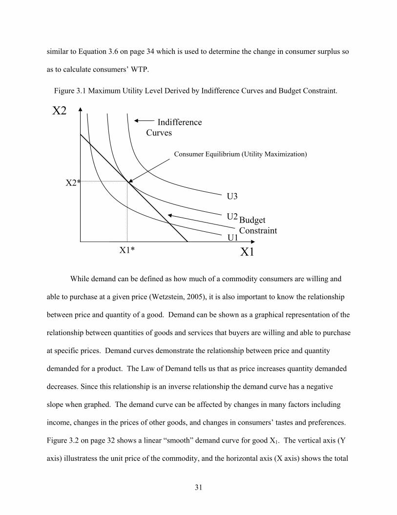
Figure 3.1 on page 31 shows the various combinations of commodity bundles that form
individual i’s indifference curves. Utility is maximized for the consumer when the ratio of the
product prices (X1 and X2) is equal to the marginal utility ratio of the consumer derives from the
products for a given budget constraint. This point is where the slope of the budget constraint is
equal to (tangent to) the slope of the consumer’s indifference curve.
The result from this maximization process yields the Marshallian demand functions
below
xi = h(P, Y) 3.2
By substituting the demand functions into Equation 3.1, the indirect utility function can be
obtained.
vi= f(Yi, PX |Si) 3.3
where Yi is individual i’s income, Si represents a vector of socioeconomic and demographic
variables of individual i, and PX is the vector of prices for XN commodities. Equation 3.3 is
31
similar to Equation 3.6 on page 34 which is used to determine the change in consumer surplus so
as to calculate consumers’ WTP.
While demand can be defined as how much of a commodity consumers are willing and
able to purchase at a given price (Wetzstein, 2005), it is also important to know the relationship
between price and quantity of a good. Demand can be shown as a graphical representation of the
relationship between quantities of goods and services that buyers are willing and able to purchase
at specific prices. Demand curves demonstrate the relationship between price and quantity
demanded for a product. The Law of Demand tells us that as price increases quantity demanded
decreases. Since this relationship is an inverse relationship the demand curve has a negative
slope when graphed. The demand curve can be affected by changes in many factors including
income, changes in the prices of other goods, and changes in consumers’ tastes and preferences.
Figure 3.2 on page 32 shows a linear “smooth” demand curve for good X1. The vertical axis (Y
axis) illustratess the unit price of the commodity, and the horizontal axis (X axis) shows the total
X2
X2*
U2
X1*
U3
U1
Budget Constraint
Indifference Curves
X1
Consumer Equilibrium (Utility Maximization)
Figure 3.1 Maximum Utility Level Derived by Indifference Curves and Budget Constraint.
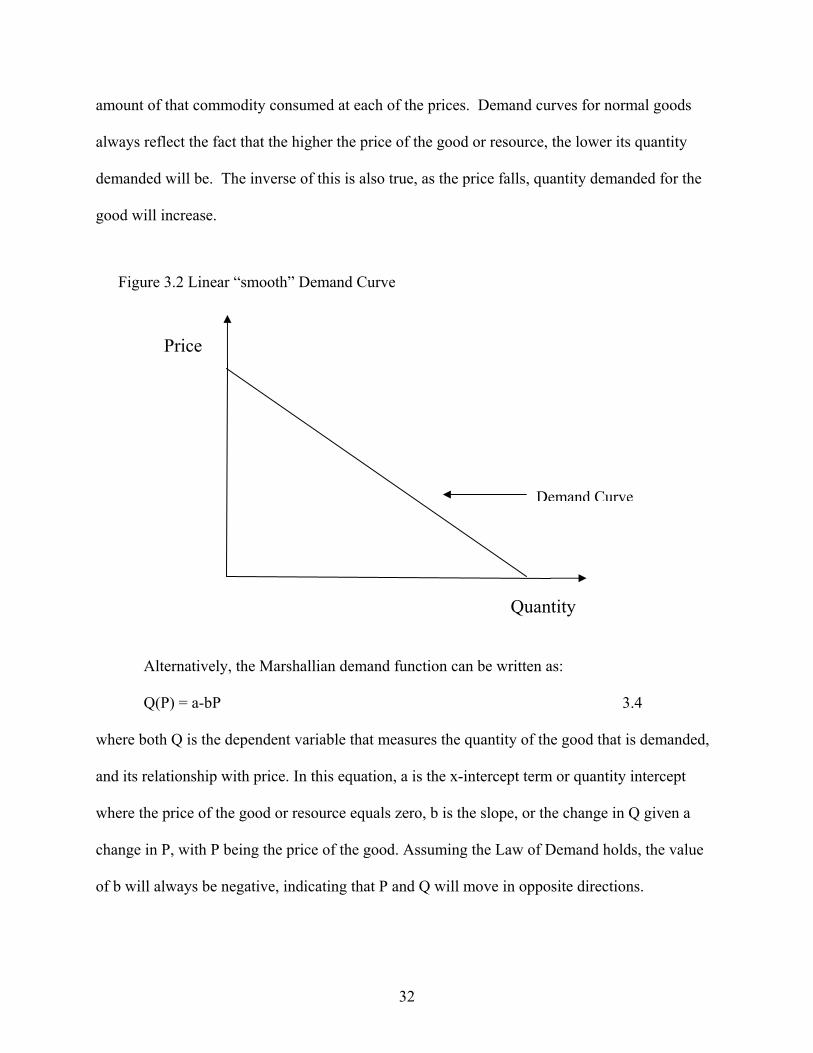
32
amount of that commodity consumed at each of the prices. Demand curves for normal goods
always reflect the fact that the higher the price of the good or resource, the lower its quantity
demanded will be. The inverse of this is also true, as the price falls, quantity demanded for the
good will increase.
Alternatively, the Marshallian demand function can be written as:
Q(P) = a-bP 3.4
where both Q is the dependent variable that measures the quantity of the good that is demanded,
and its relationship with price. In this equation, a is the x-intercept term or quantity intercept
where the price of the good or resource equals zero, b is the slope, or the change in Q given a
change in P, with P being the price of the good. Assuming the Law of Demand holds, the value
of b will always be negative, indicating that P and Q will move in opposite directions.
Price
Quantity
Demand Curve
Figure 3.2 Linear “smooth” Demand Curve

33
In order to determine the value that consumers place on goods or willingness to pay, the
inverse of the demand curve would need to be taken. The inverse demand curve describes P as a
function that is dependent on Q. The function P(Q), which is also linear, is the inverse of the
function Q(P) (www.econtools.com, 2004). The corresponding inverse demand equation is
written as
P(Q) = a-bQ 3.5
where the variables are identical to that of an ordinary demand curve. However, in Equation 3.4,
price, P, is the independent variable with quantity being dependent upon that price. In Equation
3.5, quantity, Q is independent and price is dependent upon that quantity.
Willingness to Pay
Willingness to pay (WTP) is defined as the amount that can be taken away from the
person’s income while keeping his or her utility constant in exchange for providing them a good
or service. It can also be defined as a measurement of the maximum amount of money an
individual is willing to give up to obtain a product with a quality, q or exchange a product with
quality qo for a product with quality q1 (Lusk and Hudson, 2004). Marginal willingness to pay is
another name for the Hicks-compensated inverse demand curve.
Another way of determining consumers’ WTP is to find the level of consumer surplus
associated with the product. Consumer Surplus is a method which compares the value a
consumer places on each unit of a commodity consumed against the price of that commodity.
Since there is no actual method for measuring a consumer’s utility due to the inability to quantify
changes in individual satisfaction due to price changes, consumer welfare is measured as the
difference between the maximum amount a consumer would be willing to pay and what they
34
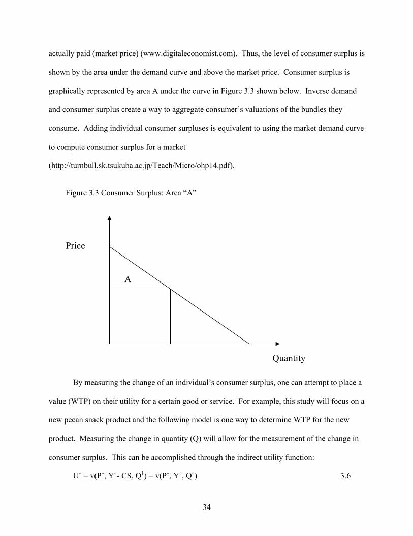
actually paid (market price) (www.digitaleconomist.com). Thus, the level of consumer surplus is
shown by the area under the demand curve and above the market price. Consumer surplus is
graphically represented by area A under the curve in Figure 3.3 shown below. Inverse demand
and consumer surplus create a way to aggregate consumer’s valuations of the bundles they
consume. Adding individual consumer surpluses is equivalent to using the market demand curve
to compute consumer surplus for a market
(http://turnbull.sk.tsukuba.ac.jp/Teach/Micro/ohp14.pdf).
By measuring the change of an individual’s consumer surplus, one can attempt to place a
value (WTP) on their utility for a certain good or service. For example, this study will focus on a
new pecan snack product and the following model is one way to determine WTP for the new
product. Measuring the change in quantity (Q) will allow for the measurement of the change in
consumer surplus. This can be accomplished through the indirect utility function:
U˚ = v(P˚, Y˚- CS, Q1) = v(P˚, Y˚, Q˚) 3.6
Figure 3.3 Consumer Surplus: Area “A”
A
Price
Quantity

35
Where, P˚ is the price of the good or service
Y˚ is the income for the individual
CS is consumer surplus
Q˚ is with no pecan snack products
Q1 is the quantity of pecan snack products.
The measure of CS is calculated by the difference in the income that allows the consumer
to be on the same indifference curve or level of utility as the initial situation. This can be
determined by using an exact welfare measure called compensation surplus. Compensation
surplus can be defined as the amount of money, paid or received, which places an individual at
his or her initial utility level after a change in quantity, where optimizing adjustments are not
allowed (Allen, 2004). By using compensation surplus, economists can determine if the benefits
from a policy change to the gainers outweigh the costs to the losers. This idea is consistent with
Pareto improvements. Individuals should have the right to the initial situation and can be
measured by using the expenditure function. The expenditure function determines the minimum
income needed to provide a general level of utility.
e = e(P, Q, U) 3.7
Where P represents price of the good
Q represents the quantity of the good
U denotes the utility level of the individual
The underlying Hicksian demand function can be defined as:
=dPde h = h(P,U) 3.8
where h is the Hicksian demand function.
36
Based on the expenditure function, the welfare measure or willingness to pay in this case
can be shown as:
WTP = C = {[e(P˚, Q1, U˚) = Y1] – [e(P˚, Q˚, U˚) = Y˚]} 3.9
= |Y1-Y˚|
Where, Q1> Q˚, and
Y˚ > Y1
Compensating surplus is the individual’s willingness to pay for a higher level of Q, or
WTP in the case of an increase in quantity. This is the Hicksian compensating welfare measure.
Compensating surplus is considered an income decrement because the individual states that they
are willing to decrease their income by some amount to remain at the initial level of the
consumption.
According to Champ et al. (2003) the expenditure function is the “ticket to welfare
economics”. The benefit of the Hicksian demand functions is that they take utility into account
whereas the Marshallian demand functions only utilize prices and quantities.
Consumer surplus can be calculated by using the Equivalent Surplus (ES). Freeman
(2003) describes ES as the change in income required, given old prices and consumption level of
a good to make an individual as well off as that person would be with the new price set and
consumption level. This is the same principal as compensating surplus; however it assigns the
rights to the subsequent quantity level, as opposed to the initial quantity level. For an imposed
quantity decrease, ES is an income decrement.
Another method of determining the WTP of a pecan snack product, a market good, is to
determine the Marshallian consumer surplus. Utility is still the basis of determining a price,
though finding the compensating surplus or equivalent surplus will not be necessary. This can be
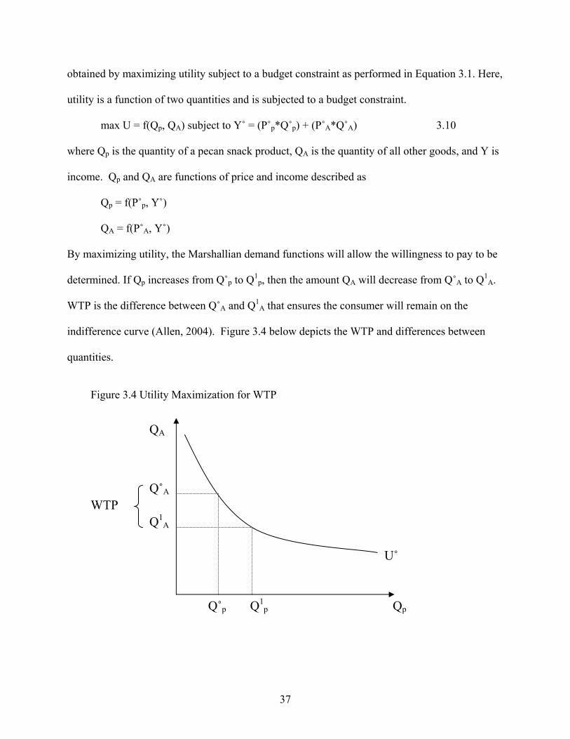
37
obtained by maximizing utility subject to a budget constraint as performed in Equation 3.1. Here,
utility is a function of two quantities and is subjected to a budget constraint.
max U = f(Qp, QA) subject to Y˚ = (P˚p*Q˚p) + (P˚A*Q˚A) 3.10
where Qp is the quantity of a pecan snack product, QA is the quantity of all other goods, and Y is
income. Qp and QA are functions of price and income described as
Qp = f(P˚p, Y˚)
QA = f(P˚A, Y˚)
By maximizing utility, the Marshallian demand functions will allow the willingness to pay to be
determined. If Qp increases from Q˚p to Q1p, then the amount QA will decrease from Q˚A to Q1
A.
WTP is the difference between Q˚A and Q1A that ensures the consumer will remain on the
indifference curve (Allen, 2004). Figure 3.4 below depicts the WTP and differences between
quantities.
Q˚A
Q1A
Qp
QA
Q˚p Q1p
Figure 3.4 Utility Maximization for WTP
U˚
WTP

38
Utilizing Contingent Valuation to Determine WTP
Contingent Valuation (CV) is the most widely used method to measure consumers’
willingness to pay. Contingent valuation is a method of estimating the value that a person places
on a good. The CV approach elicits willingness to pay (WTP) to obtain a specified good, or
willingness to accept (WTA) to give up a good directly from potential consumers rather than
inferring from observed market behaviors.
Telephone, mail surveys, or face-to-face interviews can be used to elicit consumer’s
willingness to pay for some unobservable good, given a hypothetical scenario. Consumers will
give their answers about willingness to pay for a specified level of a good, or a change in the
quality or attribute of some good.
Contingent valuation has been successfully used for commodities that are not exchanged
in regular markets, or when it is difficult to observe market transactions under desired conditions.
According to Barry Field (1994), contingent valuation has been performed most often for
environmental factors such as the value of amenities, preservation of wildlife and land,
recreational opportunities of resources, and others. More recently, however, CV has been used
for commodities available for sale in regular marketplaces such as pesticide-free produce,
certification requirements on beef and seafood, and potential products and services. There are
also many CV surveys found on food safety valuation studies (Buzby et al, 1998; Wessells and
Anderson, 1995; and Boccaletti and Nardella, 2001).
The Contingent Valuation Method is used in this study because of the need to measure
hypothetical pecan product values. Since a measure of the total economic value of pecans is
required, CV is the best option available. The first step in this approach is to calculate the
indirect utility function:

39
Vi = vi(Yi, Z, Px) + ei 3.11
Where: Yi is individual i’s income
Z is the amount of pecan snack product
Px is the price of all other goods
ei = random disturbance
It is assumed that the amount of pecan snacks is fixed at 1, so Z=1. In order to determine the
probability of a yes or no answer to the dichotomous choice questions used in the CV format, the
change in utility with and without the pecan snack product must be determined.
vi(Yi -Pz, 1, Px) :the utility associated with one pecan snack product, Pz is the price
of the pecan snack product
vi(Yi, 0, Px) :the utility associated without the pecan snack product
∆vi = [v(Yi -Pz, 1, Px) + e1] – [v(Yi, 0, Px) + e0]
if ∆vi > 0, then consumer will say ‘yes’ to the bid amount
∆vi < 0, then consumer will say ‘no’ to the bid amount
∆vi = 0, then consumer will be indifferent
In terms of probability, the probability of a YES response is:
Prob[“YES”] = Prob[∆(vi) ≥ ∆(ei)] = F[∆(vi)] 3.12
where F is the cumulative density function, CDF.
The goal of contingent valuation is to measure the compensating or equivalent variation
for some good. Compensating variation is a measure used when the person must purchase a
good. Equivalent variation is used if the person faces a loss of the good. Both variations can be
elicited by asking a person to state a willingness to pay a monetary amount for some good or
service.

40
For standard neoclassical demand theory, demand equations can be derived which
express the quantity of a particular commodity as a function of the price of the commodity,
prices of related commodities, household income and other socioeconomic variables which are
related to a systematic change in preferences (Allen, 2004). An individual’s willingness to pay
for a commodity can be expressed by the bid function:
WTP = f(Bid, Income, Education, Age, Gender, …etc). 3.13
In a contingent market using an open-ended question, maximum WTP is stated directly
by individuals. The amount of WTP is estimated for a given individual utility change. The
individual’s utility change depends upon the estimation of benefits gained from consuming a
single serving snack size bag of pecans. The benefits may vary across individuals because of
differences in income, initial offer price, socioeconomic variables, and preferences. The
equation may be specified in a linear or logarithmic form to estimate WTP for a single serving
snack size bag of pecans and estimated using ordinary least squares (OLS).
Mean WTP = E[CS]
WTP
Pr[YES]
0
Figure 3.5 Expected Consumer Surplus from Dichotomous Choice CVM
E[CSi]

41
Chapter 4
Data Collection and Results
Obtaining primary data on potential consumer purchases of agricultural commodities is
difficult at best. A consumer survey is one of the tools available to gather information about
consumer preferences and attitudes for agricultural products. In this study the contingent
valuation method is used to estimate the willingness to pay (WTP) for a 2.5 ounce single serving
snack size bag of pecans. Both simple statistical analysis and regression analysis is used to
determine the factors associated with consumers’ expected WTP for the pecan snack product. In
this case, the Tobit model was chosen for the regression portion of the analysis as the appropriate
model to analyze the data and will be explained later in the chapter.
Potential consumer purchasing behavior is assumed to be a function of several factors
including perceptions of the quality and value of the product in question, prior shopping
experiences, the consumer’s loyalty for certain nuts, as well as demographic composition of the
household. Consumer perceptions about certain products and food issues tend to be a major
factor in determining the WTP. Other sociodemographic variables such as education, income,
number of children, gender, and age could be important determinants. Residency has the
potential to affect respondents’ decisions to purchase pecan products. This is due to the regional
availability of pecans and regional respondents’ customs.
42
Survey Design
The issue of the relative influence of economic, physical, and other personal factors on a
potential pecan snack product was a question in this study. In order to obtain such data, a
nationwide survey was designed and implemented. This U.S. household survey was used due
the to regionality of pecan production. A nationwide survey allows for a national representation
of consumers. Consumer data was collected to estimate consumer willingness to pay (WTP) for a
2.5 single serving snack size bag of pecans. The survey was created and designed using the
contingent valuation method format. The CVM with a willingness to pay construction was
deemed the most efficient way to measure these values.
The data was collected by the Survey Research Center of The University of Georgia
using a computer assisted telephone interview (CATI) system. The telephone interview method
that the Survey Research Center used was a random digit dialing method. When conducting
these interviews, the selection of whom to contact in each household was done based on the
“youngest male, oldest female” technique. Essentially, the interviewer calls a phone number and
asks to speak to the youngest male, 18 years of age or older, who lives in the household. If not
available, they will then ask to speak with the oldest female who lives in the household. This
procedure tends to generate more male respondents, which are typically under represented in
sample surveys. The Survey Research Center conducted the survey during December 2004 and
January 2005 using the random digit dialing sample that yielded 913 interviews.
The survey was designed to allow only those who answered “yes” to “Have you
purchased pecans in the last 24 months?” to continue and complete the rest of the survey. If the
respondent had not purchased pecans, then the question, “Why have you not purchased pecans in
the last 24 months?” was asked and the survey ended for that particular respondent. By using this

43
format, some information about general nut consumption was obtained and more obtained for
those who had actually purchased pecans in the last two years. The Survey Research Center was
asked to obtain 500 completed surveys of those who answered “yes” to Question 4.
Since it would be expensive and very nearly impossible to have every consumer in the
United States be given the survey instrument, a sample must be taken. As the survey sample size
increases, the ability of that sample to accurately represent the population increases as well. The
rationale for asking that 500 surveys be completed was that it would set the confidence level for
the inferences made from the survey at 95 percent. To have a confidence level of 95 percent
means that the inferences made from this sample would be consistent with the population 19
times out of 20. In order for the inferences to be statistically significant at the 0.95 confidence
level, it was determined that a minimum of 480 surveys would need to be completed.
Of those 500 surveys that were requested, only 474 were useable. Once the survey results
were reviewed, an additional 136 surveys were deleted due to incomplete answers for household
income. This reduced the number of observations to 338, decreasing the overall confidence level
for the inference to 0.94. Although most researchers seem to strive for at least 95 percent
confidence, the confidence level of 94 percent attributed to this sample size is still sufficient.
Table 4.1 below shows the reasons respondents gave for not having purchased pecans in
the last 24 months. For those respondents who do not purchase pecans, 50 percent said it is due
to the fact that they just do not like the taste of pecans. Fifteen percent reported either having a
pecans tree or having friends who have trees and therefore do not need to purchase pecans.
Thirteen percent indicated being allergic or having some other medical reason. Other reasons
included the lack of availability (seven percent), pecans are too expensive (five percent), and
‘other’ (three percent).
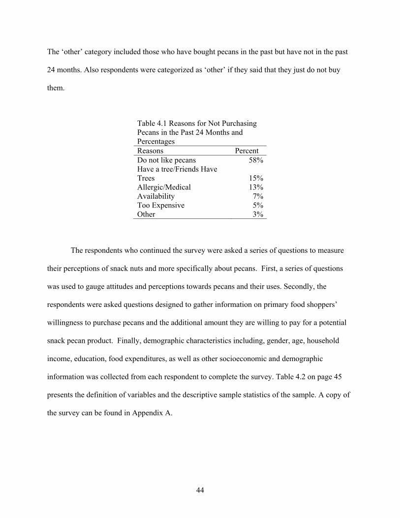
44
The ‘other’ category included those who have bought pecans in the past but have not in the past
24 months. Also respondents were categorized as ‘other’ if they said that they just do not buy
them.
The respondents who continued the survey were asked a series of questions to measure
their perceptions of snack nuts and more specifically about pecans. First, a series of questions
was used to gauge attitudes and perceptions towards pecans and their uses. Secondly, the
respondents were asked questions designed to gather information on primary food shoppers’
willingness to purchase pecans and the additional amount they are willing to pay for a potential
snack pecan product. Finally, demographic characteristics including, gender, age, household
income, education, food expenditures, as well as other socioeconomic and demographic
information was collected from each respondent to complete the survey. Table 4.2 on page 45
presents the definition of variables and the descriptive sample statistics of the sample. A copy of
the survey can be found in Appendix A.
Table 4.1 Reasons for Not Purchasing Pecans in the Past 24 Months and Percentages Reasons Percent Do not like pecans 58%Have a tree/Friends Have Trees 15%Allergic/Medical 13%Availability 7%Too Expensive 5%Other 3%
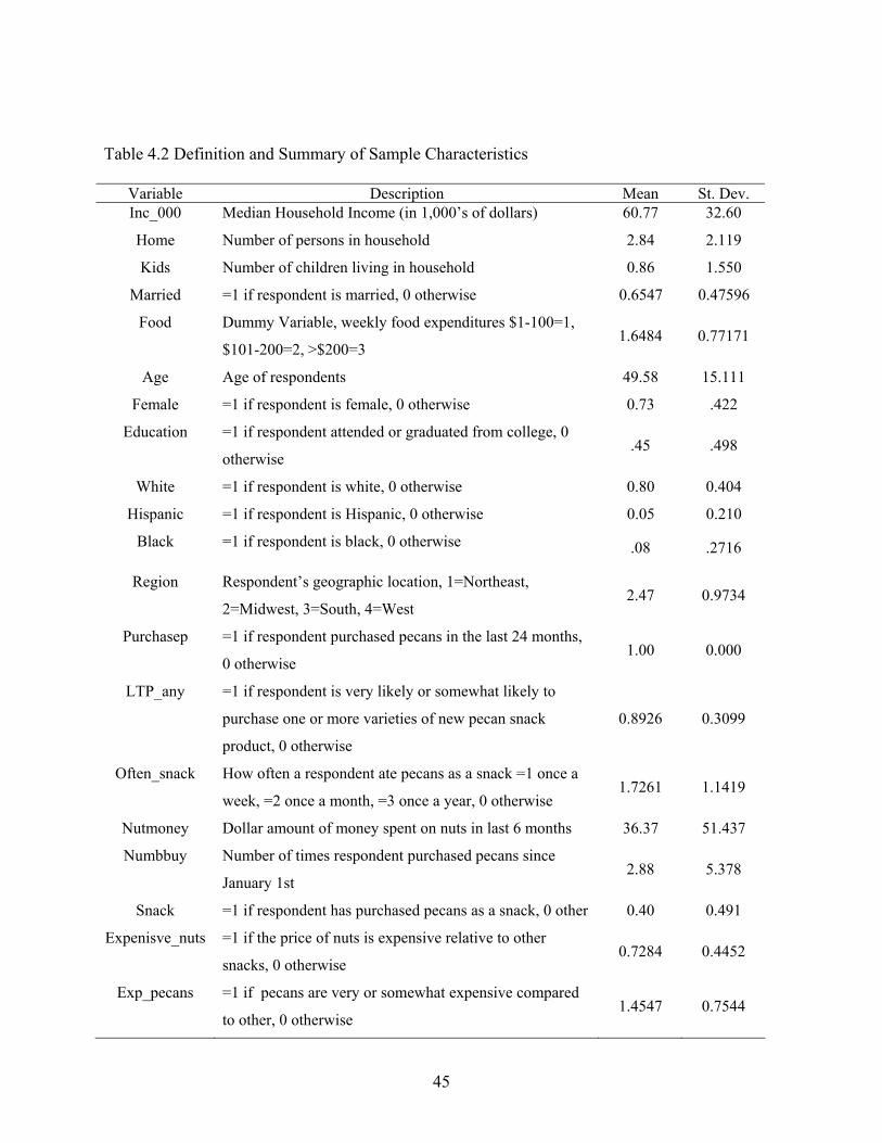
45
Table 4.2 Definition and Summary of Sample Characteristics
Variable Description Mean St. Dev. Inc_000 Median Household Income (in 1,000’s of dollars) 60.77 32.60
Home Number of persons in household 2.84 2.119
Kids Number of children living in household 0.86 1.550
Married =1 if respondent is married, 0 otherwise 0.6547 0.47596
Food Dummy Variable, weekly food expenditures $1-100=1,
$101-200=2, >$200=3 1.6484 0.77171
Age Age of respondents 49.58 15.111
Female =1 if respondent is female, 0 otherwise 0.73 .422
Education =1 if respondent attended or graduated from college, 0
otherwise .45 .498
White =1 if respondent is white, 0 otherwise 0.80 0.404
Hispanic =1 if respondent is Hispanic, 0 otherwise 0.05 0.210
Black =1 if respondent is black, 0 otherwise .08 .2716
Region Respondent’s geographic location, 1=Northeast,
2=Midwest, 3=South, 4=West 2.47 0.9734
Purchasep =1 if respondent purchased pecans in the last 24 months,
0 otherwise 1.00 0.000
LTP_any =1 if respondent is very likely or somewhat likely to
purchase one or more varieties of new pecan snack
product, 0 otherwise
0.8926 0.3099
Often_snack How often a respondent ate pecans as a snack =1 once a
week, =2 once a month, =3 once a year, 0 otherwise 1.7261 1.1419
Nutmoney Dollar amount of money spent on nuts in last 6 months 36.37 51.437
Numbbuy Number of times respondent purchased pecans since
January 1st 2.88 5.378
Snack =1 if respondent has purchased pecans as a snack, 0 other 0.40 0.491
Expenisve_nuts =1 if the price of nuts is expensive relative to other
snacks, 0 otherwise 0.7284 0.4452
Exp_pecans =1 if pecans are very or somewhat expensive compared
to other, 0 otherwise 1.4547 0.7544
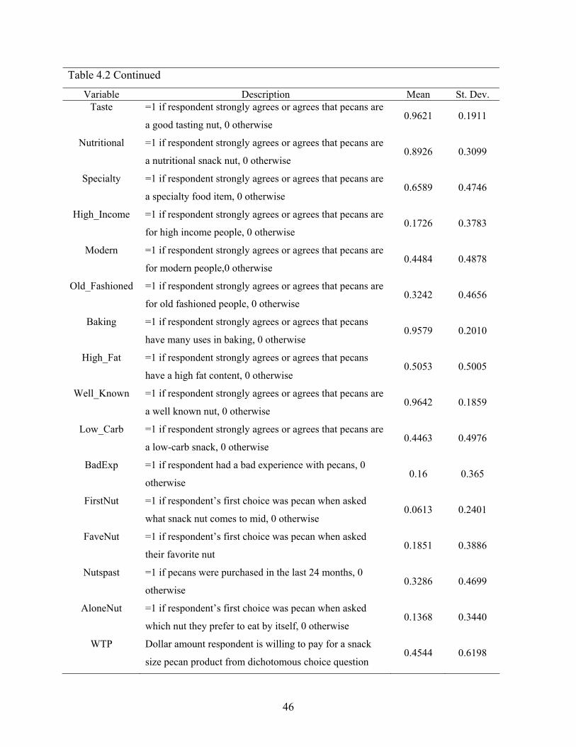
46
Table 4.2 Continued
Variable Description Mean St. Dev. Taste =1 if respondent strongly agrees or agrees that pecans are
a good tasting nut, 0 otherwise 0.9621 0.1911
Nutritional =1 if respondent strongly agrees or agrees that pecans are
a nutritional snack nut, 0 otherwise 0.8926 0.3099
Specialty =1 if respondent strongly agrees or agrees that pecans are
a specialty food item, 0 otherwise 0.6589 0.4746
High_Income =1 if respondent strongly agrees or agrees that pecans are
for high income people, 0 otherwise 0.1726 0.3783
Modern =1 if respondent strongly agrees or agrees that pecans are
for modern people,0 otherwise 0.4484 0.4878
Old_Fashioned =1 if respondent strongly agrees or agrees that pecans are
for old fashioned people, 0 otherwise 0.3242 0.4656
Baking =1 if respondent strongly agrees or agrees that pecans
have many uses in baking, 0 otherwise 0.9579 0.2010
High_Fat =1 if respondent strongly agrees or agrees that pecans
have a high fat content, 0 otherwise 0.5053 0.5005
Well_Known =1 if respondent strongly agrees or agrees that pecans are
a well known nut, 0 otherwise 0.9642 0.1859
Low_Carb =1 if respondent strongly agrees or agrees that pecans are
a low-carb snack, 0 otherwise 0.4463 0.4976
BadExp =1 if respondent had a bad experience with pecans, 0
otherwise 0.16 0.365
FirstNut =1 if respondent’s first choice was pecan when asked
what snack nut comes to mid, 0 otherwise 0.0613 0.2401
FaveNut =1 if respondent’s first choice was pecan when asked
their favorite nut 0.1851 0.3886
Nutspast =1 if pecans were purchased in the last 24 months, 0
otherwise 0.3286 0.4699
AloneNut =1 if respondent’s first choice was pecan when asked
which nut they prefer to eat by itself, 0 otherwise 0.1368 0.3440
WTP Dollar amount respondent is willing to pay for a snack
size pecan product from dichotomous choice question 0.4544 0.6198
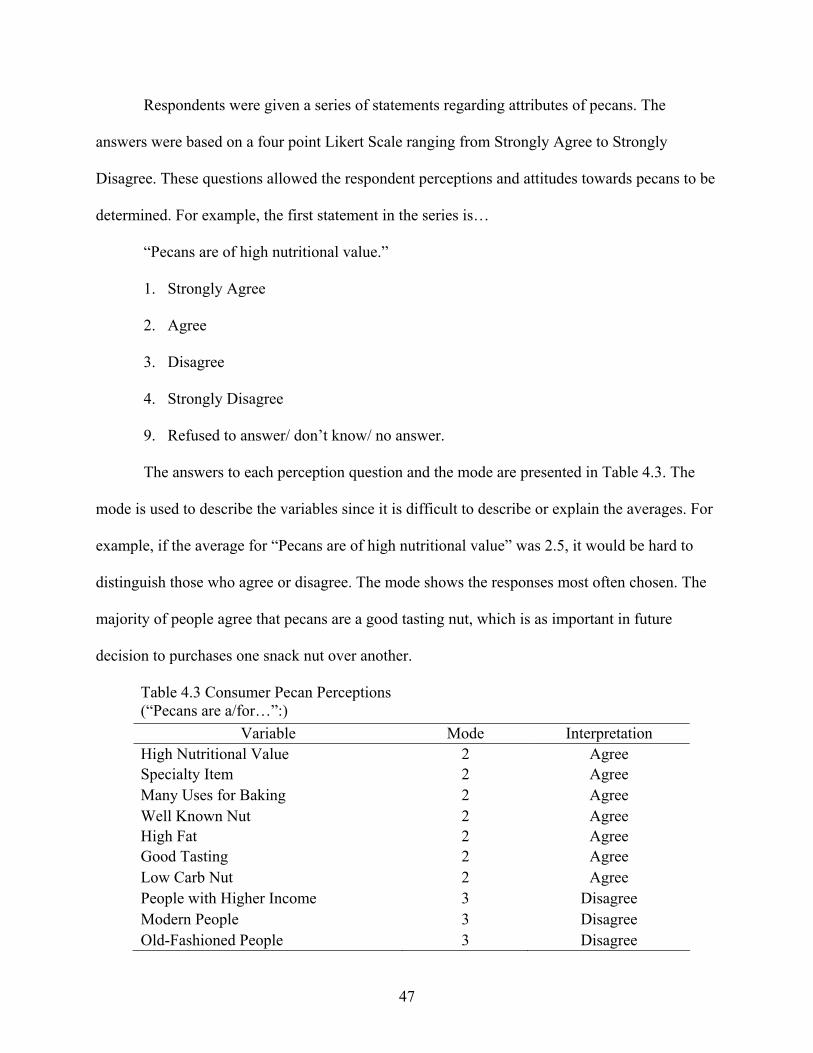
47
Respondents were given a series of statements regarding attributes of pecans. The
answers were based on a four point Likert Scale ranging from Strongly Agree to Strongly
Disagree. These questions allowed the respondent perceptions and attitudes towards pecans to be
determined. For example, the first statement in the series is…
“Pecans are of high nutritional value.”
1. Strongly Agree
2. Agree
3. Disagree
4. Strongly Disagree
9. Refused to answer/ don’t know/ no answer.
The answers to each perception question and the mode are presented in Table 4.3. The
mode is used to describe the variables since it is difficult to describe or explain the averages. For
example, if the average for “Pecans are of high nutritional value” was 2.5, it would be hard to
distinguish those who agree or disagree. The mode shows the responses most often chosen. The
majority of people agree that pecans are a good tasting nut, which is as important in future
decision to purchases one snack nut over another.
Table 4.3 Consumer Pecan Perceptions (“Pecans are a/for…”:)
Variable Mode Interpretation High Nutritional Value 2 Agree Specialty Item 2 Agree Many Uses for Baking 2 Agree Well Known Nut 2 Agree High Fat 2 Agree Good Tasting 2 Agree Low Carb Nut 2 Agree People with Higher Income 3 Disagree Modern People 3 Disagree Old-Fashioned People 3 Disagree
48
Some explanation of the variables used in this study and expectations of results are useful
before examining the results of them. A number of dummy variables needed to be created.
Dummy variables are useful in order to indicate the absence or presence of a quality or attribute
such as female/male, race, religion and other nominal scale variables (Gujarati, 2003). In general,
gender should not affect WTP (Mukhopadhaya et al., 2004). Although, eating behaviors of males
and females can be quite different. Females often times are more involved in the purchasing and
handling of food products. Therefore, the female consumption and purchasing of snacks may be
different from that of males. Food purchases and consumption can also be closely related to
ethnicity, race, and culture of respondents.
AGE was considered to be an important factor and was computed based on the
participant’s response to a question asking the respondent to specify their age, in years. From
Rimal and Fletcher’s (2002) study on snack peanuts it can be expected that as the respondent’s
age increases, the amount she/he is willing to pay will increase.
The household income variable, INC_000, represents the respondent’s self-reported
household income (before taxes) category levels in 2003. The variable was recorded from eleven
ranges of income. The ranges were then grouped into four smaller ranges and the mid point was
taken for each group. This allows one to use an actual dollar amount rather than the range which
is preferred by economists to be able to explain the effects of income on the dependent variable.
These numbers were then divided by 1,000 to reduce the magnitude between variables and allow
the coefficients to be more manageable. It is expected that respondents with higher income will
pay more for a snack size bag of pecans.
The survey recorded the state that each respondent resided in and was then grouped into
regions. These regions were coded as follow: 1=Northeast, 2= Midwest, 3=South and 4=West. It

49
is thought that those residing in regions further away from where pecans are produced and
readily available may be willing to pay more for the snack product.
A weekly food expenditure variable, FOOD, was created in order to determine if those
households who spend more on weekly food purchases will be willing to pay more for a snack
product. Other studies have found that those with more members in the household may not
necessarily be willing to pay more for an item due to the amount of money spent per person on
food (see Govindasamy and Italia, 1998).
Several dummy variables were included to account for respondents’ attitudes and
perceptions towards nuts and pecans in particular. For example, if a person believes that pecans
are a good tasting nut, they may be more likely to purchase a snack size bag of pecans. If pecans
are their favorite nut, they may be willing to pay more for the snack product. FAVENUT is a
dummy variable that assigns a one to those who said that pecans were one of their favorite nuts.
The survey also asked the respondents how many times since January 1st they have purchased
pecans, NUMBBUY. Those who purchase pecans more often throughout the year may be willing
to pay more.
A series of questions were asked in similar fashion to the ones that used the Likert Scale
discussed earlier. These questions consisted of various flavors and coatings of pecans that could
potentially be offered in a snack size bag. Each respondent was asked how likely they would be
to purchases each of these types of pecans: flavored such as chocolate or honey mustard, salted,
spicy, roasted, glazed, sugar and spice, or raw. They were asked if they would be very likely,
somewhat likely, unlikely, or very unlikely. If a respondent answered “very likely” or
“somewhat likely,” then the respondent is considered likely to buy at least one of the varieties of
50
pecan snack products. For those individuals a dummy variable, LTP_ANY, is assigned a value of
1, and would receive a 0 for any other response.
Empirical analyses were performed using the dollar values for the willingness to pay
dependent variable. The dependent variable is considered to be a censored variable. It is
considered censored data because the actual WTP for a person who did not accept any bid was
not asked. Those respondents were assigned a zero, when in fact they may have been willing to
pay some price other then the choices offered. The question that was not asked was: how much
more are you willing to pay over the specified bid amount? The censoring limits differ by
individuals, and a Tobit regression model was estimated to take into account this censoring to
avoid biased and inconsistent estimates of the parameters in the model.
Willingness to pay was elicited by using the dichotomous choice format. Beginning
values were randomly assigned to each respondent and are as follows: $0.79, $0.99, $1.19,
$1.39, $1.59. Using $0.99 as an example, the respondent was asked “Would you be willing to
pay $0.99 for a 2.5 ounce single serving snack pecan product?” A second question is then asked
in regards to the answer to the first question. If the respondent answered “yes” to the first price,
they were then asked if they would be willing to pay a predetermined 25 percent price increase.
In this case the person would be asked if they would be willing to pay $1.24; the answer is
recorded and the surveyor moves on to the next question. If the answer to the first question
asking the person if they would pay $0.99 is “no”, the respondent is asked if they would be
willing to pay a predetermined 25 percent price decrease. In this case, the person would be asked
if they would be willing to pay $0.74 for the single serving snack bag of pecans. Again, the
response is recorded and the questioner moves on to the next question. Table 4.4 on the next
page presents the descriptive statistics of the willingness to pay questions.
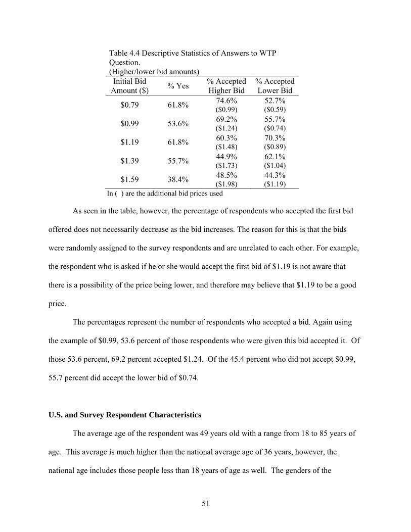
51
Table 4.4 Descriptive Statistics of Answers to WTP Question. (Higher/lower bid amounts)
Initial Bid Amount ($) % Yes % Accepted
Higher Bid % Accepted Lower Bid
$0.79 61.8% 74.6% ($0.99)
52.7% ($0.59)
$0.99 53.6% 69.2% ($1.24)
55.7% ($0.74)
$1.19 61.8% 60.3% ($1.48)
70.3% ($0.89)
$1.39 55.7% 44.9% ($1.73)
62.1% ($1.04)
$1.59 38.4% 48.5% ($1.98)
44.3% ($1.19)
In ( ) are the additional bid prices used
As seen in the table, however, the percentage of respondents who accepted the first bid
offered does not necessarily decrease as the bid increases. The reason for this is that the bids
were randomly assigned to the survey respondents and are unrelated to each other. For example,
the respondent who is asked if he or she would accept the first bid of $1.19 is not aware that
there is a possibility of the price being lower, and therefore may believe that $1.19 to be a good
price.
The percentages represent the number of respondents who accepted a bid. Again using
the example of $0.99, 53.6 percent of those respondents who were given this bid accepted it. Of
those 53.6 percent, 69.2 percent accepted $1.24. Of the 45.4 percent who did not accept $0.99,
55.7 percent did accept the lower bid of $0.74.
U.S. and Survey Respondent Characteristics
The average age of the respondent was 49 years old with a range from 18 to 85 years of
age. This average is much higher than the national average age of 36 years, however, the
national age includes those people less than 18 years of age as well. The genders of the
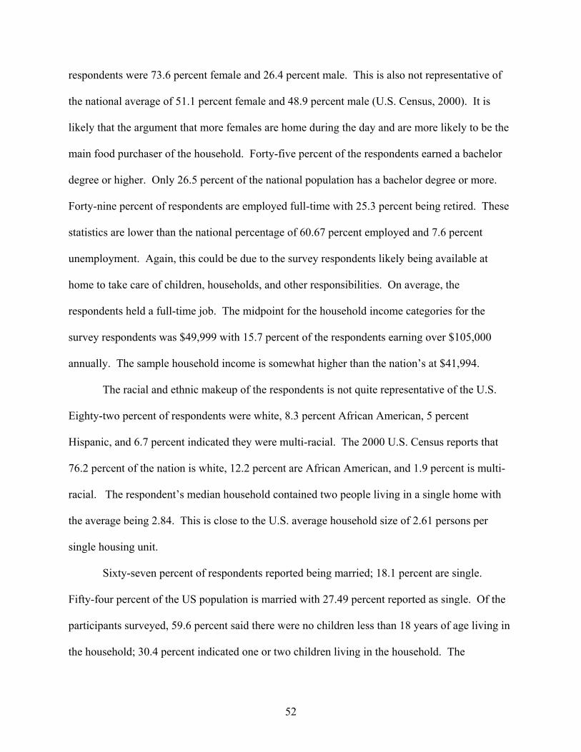
52
respondents were 73.6 percent female and 26.4 percent male. This is also not representative of
the national average of 51.1 percent female and 48.9 percent male (U.S. Census, 2000). It is
likely that the argument that more females are home during the day and are more likely to be the
main food purchaser of the household. Forty-five percent of the respondents earned a bachelor
degree or higher. Only 26.5 percent of the national population has a bachelor degree or more.
Forty-nine percent of respondents are employed full-time with 25.3 percent being retired. These
statistics are lower than the national percentage of 60.67 percent employed and 7.6 percent
unemployment. Again, this could be due to the survey respondents likely being available at
home to take care of children, households, and other responsibilities. On average, the
respondents held a full-time job. The midpoint for the household income categories for the
survey respondents was $49,999 with 15.7 percent of the respondents earning over $105,000
annually. The sample household income is somewhat higher than the nation’s at $41,994.
The racial and ethnic makeup of the respondents is not quite representative of the U.S.
Eighty-two percent of respondents were white, 8.3 percent African American, 5 percent
Hispanic, and 6.7 percent indicated they were multi-racial. The 2000 U.S. Census reports that
76.2 percent of the nation is white, 12.2 percent are African American, and 1.9 percent is multi-
racial. The respondent’s median household contained two people living in a single home with
the average being 2.84. This is close to the U.S. average household size of 2.61 persons per
single housing unit.
Sixty-seven percent of respondents reported being married; 18.1 percent are single.
Fifty-four percent of the US population is married with 27.49 percent reported as single. Of the
participants surveyed, 59.6 percent said there were no children less than 18 years of age living in
the household; 30.4 percent indicated one or two children living in the household. The

53
percentage of the US households reporting at least one child less than 18 years of age in a
household is 35.44 percent. Food expenditures for households were requested and 23.3 percent
of respondents spend between $76 and $100 weekly for food.
The survey was administered to a national sample, and was broken down into four
regions: West, Northeast, Midwest, and South. The percentage of respondents from the groups
above are listed, respectively 19.6 percent, 28 percent, 36.2 percent, and 14.7 percent. For the
narrowed population of 343 respondents who were asked to continue the survey, the
representations of the four regions are a bit skewed to the South. This could be due to the
availability of pecans in the South creating greater Southern consumer access to purchases.
Fourteen percent, 18.4 percent, 28.6 percent, and 39.1 percent of the participants live in the
West, Northeast, Midwest, and the South respectively.
One of the objectives of this thesis is to construct a demographic profile of pecan
consumers. The survey was designed to screen out respondents that have not purchased pecans
during the previous 24 months. The reason for screening out these individuals was they could not
provide the types of information we were looking to collect since they do not purchase or eat
pecans regularly. The survey instrument included a number of demographic questions that can
be compared against the U.S. population to determine whether the two populations are
demographically similar.
Survey Respondent Characteristics of Pecan Snack Consumers
The survey methodology was designed to incorporate a random sampling procedure to
ensure a random sample of the U.S. population. The random sampling procedure ensures that
every person in the United States with a phone number has an equal chance of being contacted

54
for the survey. This allows one to look for differences in the characteristics of those respondents
who consume pecans on a regular basis to the rest of the general population. These differences
would enable a pecan processor to target consumers that fit a specific demographic profile.
Table 4.5 on the following page, provides a demographic profile of consumers who
indicated they eat pecans as a snack, once a month or more. This is a sub-sample of 206
respondents from those who indicated they have purchased pecans in the last 24 months. The
demographic information collected on these individuals are compiled and then compared to
corresponding 2000 U.S. Census data. The survey collected information on consumers who have
purchased pecans over the last year; however, there is a core group of consumers that eat pecans
on a regular basis. These consumers who purchase pecans frequently are more likely to purchase
new pecan snack products.
The frequent pecan consumer is older than the average American being somewhere
between 35-54 years old, with the median being 52 years old which is significantly older than the
U.S. population median age of 35 years. Female pecan snack consumers comprise 72 percent of
the respondents. This is not surprising given that females are more likely to purchase groceries
than are males. However, it is important when marketing products to take into account female
perceptions of the new snack product as they appear to be the gate keeper to the family.
The midpoint of the household income categories of the frequent pecan snack consumer
is $49,999 which is noticeably higher than the median for the U.S., $41,994. The income data
suggests that consumers whose household income is less than $15,000 annually are not as likely
to purchase pecans as a snack as are more affluent consumers. The income data also suggest that
affluent consumers, those whose annual household income exceeds $105,000 are more likely to
purchase pecans for a snack.

55
Table 4.5 Frequency of Purchasing Pecans as a Snack (206 Respondents)
Demographic Variables Eat Pecans More than Once a Month US Population
Age 18-19 4% 7.4% * 20-34 13% 16% 35-54 42% 34% 55-64 21% 10% 65+ 23% 12%
Mean 52 years 35 years Gender
Male 28% 49% Female 72% 51%
Household Income Less than $15,000 3% 16% $15,000 - $24,999 11% 13% $25,000 - $34,999 10% 13% $35,000 - $44,999 18% 17% ($35-$49K) $45,000 - $54,999 13% -- $55,000 - $64,999 9% -- $65,000 - $74,999 6% 20% ($50-$75K) $75,000 - $84,999 6% -- $85,000 - $94,999 4% -- $95,000 - $104,999 3% 10% ($75-99K) $105,000 or more 18% 12% (>$100K)
Median $49,999 $41,994 Education
Less than high school degree 3% 20%** High school diploma/GED 22% 29% Some college/technical school 29% 21% College graduate 35% 22% Post-graduate degree 10% 9%
Race/Ethnicity White 74% 75% Black 11% 12% Asian 1% 4% American Indian 4% 1% Multi-racial 6% 2% Hispanic 5% 5%
Marital Status Married 61% 54%*** Divorced 9% 10% Separated 0% 2% Widowed 10% 7% Single 20% 27%

56
Table 4.5 Frequency of Purchasing Pecans as a Snack
Demographic Variables Eat Pecans More than Once a Month US Average
Region Northeast 18% 22% Midwest 21% 22% South 44% 31% West 17% 25%
*this percentage is for ages 15-19, only data available ** Ages 25 and older ***Ages 15 and older
Examining the educational attainment data reveals that frequent pecan snack consumers
are more educated than the U.S. population as whole. Frequent pecan snack consumers are
significantly more likely to have attained a degree in higher education, 45 percent, than U.S.
population where only 31 percent have a bachelor’s degree.
In terms of race and ethnicity, the White, Black, and Hispanic populations are similar to
those of the national average. According to the responses, Asians are less likely to purchase
pecans and Native Americans and people of Multi-racial backgrounds are more likely to
purchase pecans. Married and Widowed people are more likely to purchase pecans as a snack
while Single and Separated people are less likely. Northeasterners and Westerners are not as
likely to purchase pecans as are Southerners.
From analyzing the demographic data of the frequent pecan purchasers one can conclude
that the average consumer is older, more affluent and educated. This is a good profile and
suggests that pecans are not being consumed by younger Americans. It would be appropriate for
the pecan industry to focus on marketing strategies to younger consumers to increase the demand
for pecans. Also, pecan snacks need to be heavily marketed and promoted in the Northeast and
Western U.S. as they are less likely than Southerners to eat pecans on a regular basis.

57
Additional Demographic Characteristic Analysis
In addition to the above demographic profile, more information can be gleaned from the
survey results using cross tabular analysis. Table 4.6 on below shows the results from the type
of store or where pecans are purchased by the regions where the consumers live. From this table
it can be seen that most individuals across the United States tend to buy most of there pecans at
the grocery store. Eighteen percent of the consumers in the South said that they purchase pecan
at some other place than the five locations that were given as possible places.
Table 4.6 Places Pecans are Purchased the most By Region Northeast Midwest South West Grocery store 83% 80% 69% 76% Catalog order 0% 0% 1% 0% Specialty store 5% 5% 5% 9% Through a fund-raiser 2% 3% 4% 0% Road side stand 0% 4% 4% 1% Other 10% 8% 18% 14%
Table 4.7 shows the consumers’ mean willingness to pay for a 2.5 ounce snack pack of
pecans at the four different income categories. The willingness to pay was highest for the
income level of $49,999.50 at $0.95, with the lowest being for both the highest and lowest
income levels at $0.91.
Table 4.7 WTP for each Income Level Income Level WTP $17,499.49 $ 0.91 $49,999.50 $ 0.95 $79,999.50 $ 0.94 $109,999.50 $ 0.91
It was thought that the region that a consumer lived in would also have an effect on their
mean willingness to pay for a pecan snack product. According to the results shown in Table 4.8,
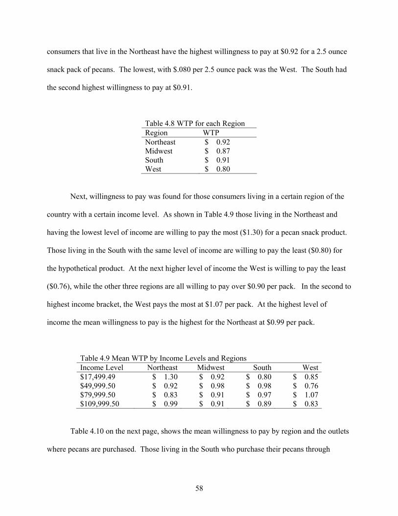
58
consumers that live in the Northeast have the highest willingness to pay at $0.92 for a 2.5 ounce
snack pack of pecans. The lowest, with $.080 per 2.5 ounce pack was the West. The South had
the second highest willingness to pay at $0.91.
Table 4.8 WTP for each Region Region WTP Northeast $ 0.92 Midwest $ 0.87 South $ 0.91 West $ 0.80
Next, willingness to pay was found for those consumers living in a certain region of the
country with a certain income level. As shown in Table 4.9 those living in the Northeast and
having the lowest level of income are willing to pay the most ($1.30) for a pecan snack product.
Those living in the South with the same level of income are willing to pay the least ($0.80) for
the hypothetical product. At the next higher level of income the West is willing to pay the least
($0.76), while the other three regions are all willing to pay over $0.90 per pack. In the second to
highest income bracket, the West pays the most at $1.07 per pack. At the highest level of
income the mean willingness to pay is the highest for the Northeast at $0.99 per pack.
Table 4.9 Mean WTP by Income Levels and Regions Income Level Northeast Midwest South West $17,499.49 $ 1.30 $ 0.92 $ 0.80 $ 0.85 $49,999.50 $ 0.92 $ 0.98 $ 0.98 $ 0.76 $79,999.50 $ 0.83 $ 0.91 $ 0.97 $ 1.07 $109,999.50 $ 0.99 $ 0.91 $ 0.89 $ 0.83
Table 4.10 on the next page, shows the mean willingness to pay by region and the outlets
where pecans are purchased. Those living in the South who purchase their pecans through

59
Table 4.10 Mean WTP by Region and Where Pecans Most Often Purchased Northeast Midwest South West Grocery Store $ 0.94 $ 0.92 $ 0.97 $ 0.90 Specialty Store $ 0.58 $ - $ 0.84 $ 0.72 Fund-Raiser $ 0.37 $ 0.98 $ 1.22 $ - Roadside Stand $ - $ 0.73 $ 0.99 $ - Other $ 1.09 $ 1.00 $ 0.67 $ -
fundraisers tend to be willing to pay more ($1.22) per pack. According to the table, there is not
much difference between regions when looking at the willingness to pay for a pecan snack
product and those who purchase pecans at grocery stores.
The following table is similar to Table 4.10 except that region has been replaced with
income level. According to Table 4.11, those consumers with an income level of $49,999.50
who purchase pecans through fundraisers would be willing to pay the most for a pecan snack
product. Their mean willingness to pay was estimated to be $1.39 per pack. Consumers who
purchase pecans at roadside stands and through fund-raisers in the mid-income groups may be a
target market due to their higher mean willingness to pay.
Table 4.11 Mean WTP by Income Level and Where Pecans Most Often Purchased $17,499.49 $49,999.50 $79,999.50 $109,999.50 Grocery Store $ 1.05 $ 0.98 $ 1.00 $ 0.88 Specialty Store $ - $ - $ - $ 0.97 Fund-Raiser $ 0.99 $ 1.39 $ 1.29 $ 1.23 Roadside Stand $ - $ 1.17 $ 1.24 $ 0.62 Other $ 0.86 $ - $ 0.78 $ 0.91
Table 4.12 on the following page shows the mean willingness to pay for a pecan snack
product by the level of income and size of packaging most often purchased. Those who purchase
a quarter pound bag of pecans and whose income level is $49,999.50 have the highest mean
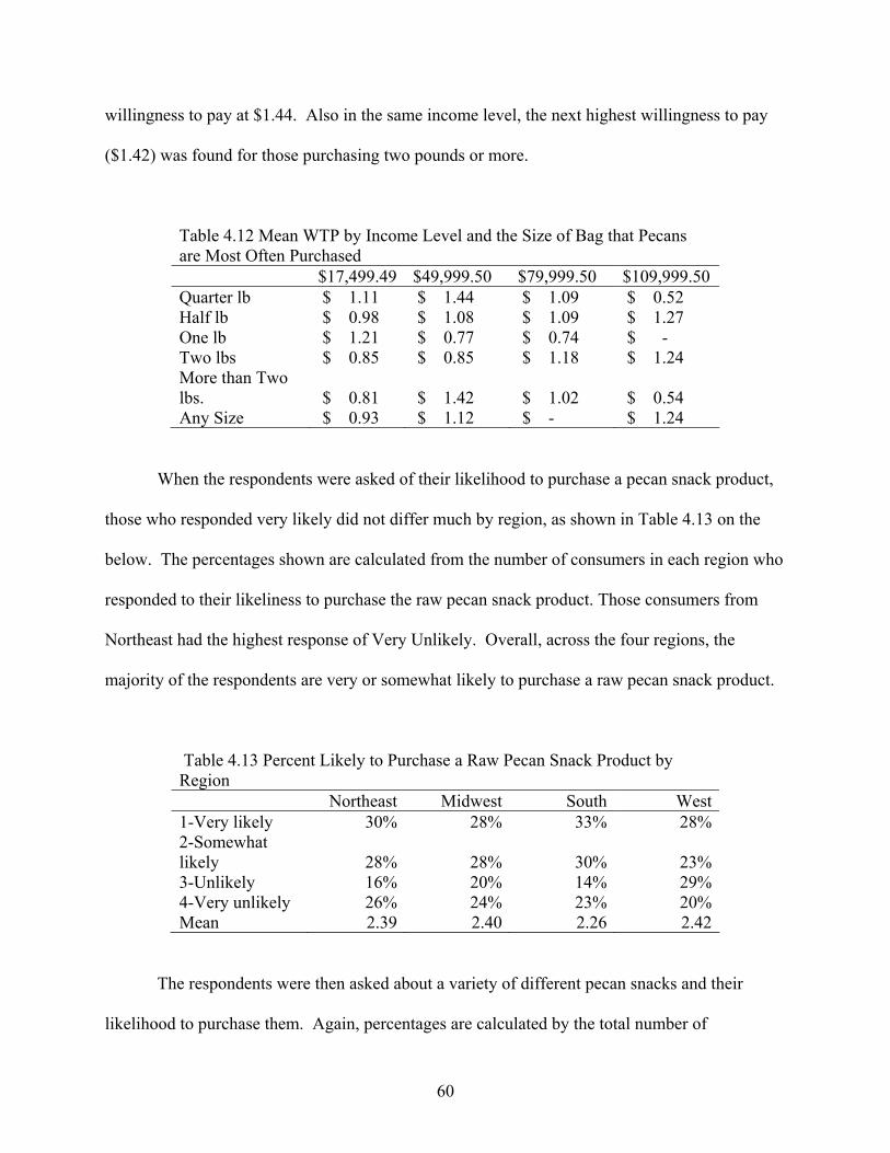
60
willingness to pay at $1.44. Also in the same income level, the next highest willingness to pay
($1.42) was found for those purchasing two pounds or more.
Table 4.12 Mean WTP by Income Level and the Size of Bag that Pecans are Most Often Purchased $17,499.49 $49,999.50 $79,999.50 $109,999.50 Quarter lb $ 1.11 $ 1.44 $ 1.09 $ 0.52 Half lb $ 0.98 $ 1.08 $ 1.09 $ 1.27 One lb $ 1.21 $ 0.77 $ 0.74 $ - Two lbs $ 0.85 $ 0.85 $ 1.18 $ 1.24 More than Two lbs. $ 0.81 $ 1.42 $ 1.02 $ 0.54 Any Size $ 0.93 $ 1.12 $ - $ 1.24
When the respondents were asked of their likelihood to purchase a pecan snack product,
those who responded very likely did not differ much by region, as shown in Table 4.13 on the
below. The percentages shown are calculated from the number of consumers in each region who
responded to their likeliness to purchase the raw pecan snack product. Those consumers from
Northeast had the highest response of Very Unlikely. Overall, across the four regions, the
majority of the respondents are very or somewhat likely to purchase a raw pecan snack product.
Table 4.13 Percent Likely to Purchase a Raw Pecan Snack Product by Region Northeast Midwest South West 1-Very likely 30% 28% 33% 28% 2-Somewhat likely 28% 28% 30% 23% 3-Unlikely 16% 20% 14% 29% 4-Very unlikely 26% 24% 23% 20% Mean 2.39 2.40 2.26 2.42
The respondents were then asked about a variety of different pecan snacks and their
likelihood to purchase them. Again, percentages are calculated by the total number of

61
respondents in each region and according to their likeliness to purchase each variety of pecan
snack product. Tables 4.14 through 4.19 show the results. Table 4.14 shows that a small
proportion of respondents were not very likely to purchase a sugar and spice pecan snack
product. These responses were not different by region as well. A larger proportion of the
respondent in all regions stated that they were more unlikely to purchase this pecan snack than
likely.
Table 4.14 Percent Likely to Purchase a Sugar and Spice Pecan Snack Product by Region Northeast Midwest South West 1-Very likely 15% 14% 17% 15% 2-Somewhat likely 29% 22% 28% 22% 3-Unlikely 22% 34% 25% 33% 4-Very unlikely 34% 30% 30% 30% Mean 2.75 2.81 2.67 2.78
The percentages in Table 4.15 show that across all regions, the majority of consumers are
very or somewhat likely to purchase a roasted pecan snack product. Thirty-five percent of those
living in the South have the highest percentage of those very likely to purchase this particular
variety.
Table 4.15 Percent Likely to Purchase a Roasted Pecan Snack Product by Region Northeast Midwest South West 1-Very likely 26% 29% 35% 30% 2-Somewhat likely 42% 43% 44% 45% 3-Unlikely 14% 12% 9% 16% 4-Very unlikely 18% 16% 12% 9% Mean 2.24 2.14 1.98 2.04

62
The next table describes the percentage of respondents who are likely to purchase a
flavored pecans snack product such as chocolate covered or honey mustard. According to Table
4.16, those living in the Northeast are evenly divided in their likelihood to purchase a flavored
pecans snack product. The highest mean WTP belongs in the category of those living in the
South and reporting they are somewhat likely to purchase a flavored product.
Table 4.16 Percent Likely to Purchase a Flavored Pecan Snack Product by Region Northeast Midwest South West 1-Very likely 20% 16% 20% 17% 2-Somewhat likely 33% 38% 39% 26% 3-Unlikely 25% 18% 19% 27% 4-Very unlikely 22% 28% 22% 30% Mean 2.48 2.59 2.43 2.71
Table 4.17 below represents the percentage of pecan consumers’ likelihood to purchase a
salted pecan snack product. The percentages are similarly dispersed among each region with the
majority likely to purchase the salted variety.
Table 4.17 Percent Likely to Purchase a Salted Pecan Snack Product by Region Northeast Midwest South West 1-Very likely 19% 21% 26% 23% 2-Somewhat likely 37% 34% 37% 34% 3-Unlikely 22% 19% 20% 23% 4-Very unlikely 22% 26% 17% 20% Mean 2.47 2.50 2.29 2.40
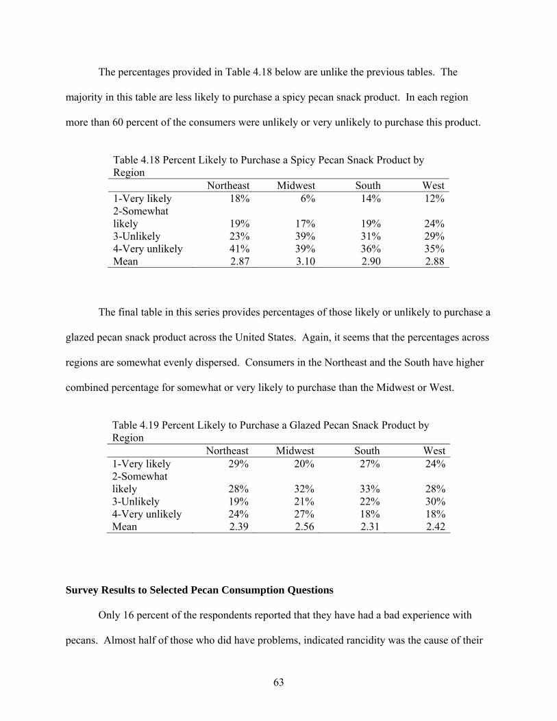
63
The percentages provided in Table 4.18 below are unlike the previous tables. The
majority in this table are less likely to purchase a spicy pecan snack product. In each region
more than 60 percent of the consumers were unlikely or very unlikely to purchase this product.
Table 4.18 Percent Likely to Purchase a Spicy Pecan Snack Product by Region Northeast Midwest South West 1-Very likely 18% 6% 14% 12% 2-Somewhat likely 19% 17% 19% 24% 3-Unlikely 23% 39% 31% 29% 4-Very unlikely 41% 39% 36% 35% Mean 2.87 3.10 2.90 2.88
The final table in this series provides percentages of those likely or unlikely to purchase a
glazed pecan snack product across the United States. Again, it seems that the percentages across
regions are somewhat evenly dispersed. Consumers in the Northeast and the South have higher
combined percentage for somewhat or very likely to purchase than the Midwest or West.
Table 4.19 Percent Likely to Purchase a Glazed Pecan Snack Product by Region Northeast Midwest South West 1-Very likely 29% 20% 27% 24% 2-Somewhat likely 28% 32% 33% 28% 3-Unlikely 19% 21% 22% 30% 4-Very unlikely 24% 27% 18% 18% Mean 2.39 2.56 2.31 2.42
Survey Results to Selected Pecan Consumption Questions
Only 16 percent of the respondents reported that they have had a bad experience with
pecans. Almost half of those who did have problems, indicated rancidity was the cause of their

64
bad experience (45.9 percent). Other reasons included a flavor different than expected (20.3
percent); piece of shell in pecans (14.9 percent), color was different than expected (1.4 percent),
and smaller than expected (4.1 percent).
Eighty-nine percent of the survey participants indicated they would be likely to purchase
some form of pecan snack product. As discussed previously in the chapter, a dummy variable
was used to describe those who are likely to purchase a pecan snack product.
During the survey interview, participants were asked if they have purchased pecans for a
gift, for a snack, or for cooking or baking. A follow up question was then asked as to which
form of pecans they purchase for each purpose. Only 8.4 percent indicated they have purchased
pecans as a gift. Less than 11 percent reported purchasing pecans as a snack and 22.5 percent for
cooking and baking purposes. The majority of respondents indicated they purchase pecan halves
for each use.
Survey respondents were asked several questions about how much they pay, where they
purchase their pecans, and how they store them. The average price per pound of pecan halves
reported was $4.50. This reported price was much lower than the average retail price of $9.00
per pound in 2005. The following statistics include all forms of pecans. Eighteen percent prefer
to purchase pecan halves opposed to in-shell, pieces, or granules. Seventy-six percent prefer to
purchase their pecans from the grocery store, and 41.6 percent reported only purchasing pecans
during the holidays (Thanksgiving, Christmas, and New Years) and special occasions. Thirty-
three percent responded to purchasing pecans on a regular basis throughout the year. These
statistics include all forms of pecans.
Survey participants were also queried on their purchase decision on snacks and snack
nuts. When asked if the respondent has ever purchased a single serving snack size bag of nuts,

65
31.4 percent have said they have purchased almonds. Cashews were second with 22.5 percent,
peanuts follow with 15.7 percent, pecans and macadamia nuts were close with 2.3 percent and
2.1 percent receptively. Other nuts mentioned were purchased at one percent or less.
Respondents were also asked how they perceived the price of snack nuts compared to
other snack foods such as chips, cookies, etc. Forty-six percent felt that snack nuts were
somewhat more expensive compared to other snack products. Twenty-nine percent believe that
snack nuts are expensive or very expensive compared to other snack products. Survey
respondents were also asked what they believed the price of pecans was compared to other snack
nuts. Nearly half, 46.2 percent, of respondents felt that pecans were priced about the same as
other snack nuts, with 40 percent and 6.5 percent believing they are more expensive or less
expensive respectively. During the survey interview the respondents were asked where they
most often purchased snack nuts. The response was a majority purchase them at the grocery
store, 58.5 percent. Other responses included convenience stores, gas stations, and vending
machines with the following respective percentages 22.4, 9.0, and 4.9.
When asked how often the respondents eat pecans as a snack, 35.3 percent replied they
eat pecans as a snack about once a year. Only 16.8 percent said they eat pecans once a week as a
snack. Fifty-seven percent reported eating roughly one handful of pecans in one sitting. An
average handful was determined to be about two ounces of pecans or about ten pecan halves.

66
Chapter 5
Empirical Results and Analysis
Overview of the Tobit Model
The Tobit model, named after James Tobin, is an extension of the Probit model and is
one approach to dealing with censored data. Censored data as defined by Gujarati (2003) is “a
sample in which information on the regressand is available only for some observations”. In other
words, y = y* if y* falls in some range and y = some limit values otherwise. The Tobit model
assumes observed consumption of a good by household i, yi, is determined by a latent variable,
y *i , that can be modeled as a linear function of a vector of independent variables Xi, a vector of
coefficients β, and an error ei, which has the normal distribution N(0, σ2). Observed consumption
can be described as follows:
yi = y *i = X `
i β + ei if X `i β > - ei
yi = 0 if X `i β ≤ - ei i = 1,2,…,N 5.1
This is a censored regression model because it is possible to view the problem as one
where observations of y* at or below zero are censored (Johnston and DiNardo, 1997).
According to McDonald and Moffitt (1980), the model assumes there is an underlying stochastic
index equal to X `i β + ei which is observed only when it is positive. Therefore, McDonald and
Moffitt (1980) believe this qualifies as an unobserved latent variable. The expected value of y in
the model is
E[y] = X `i βФ+ σф 5.2
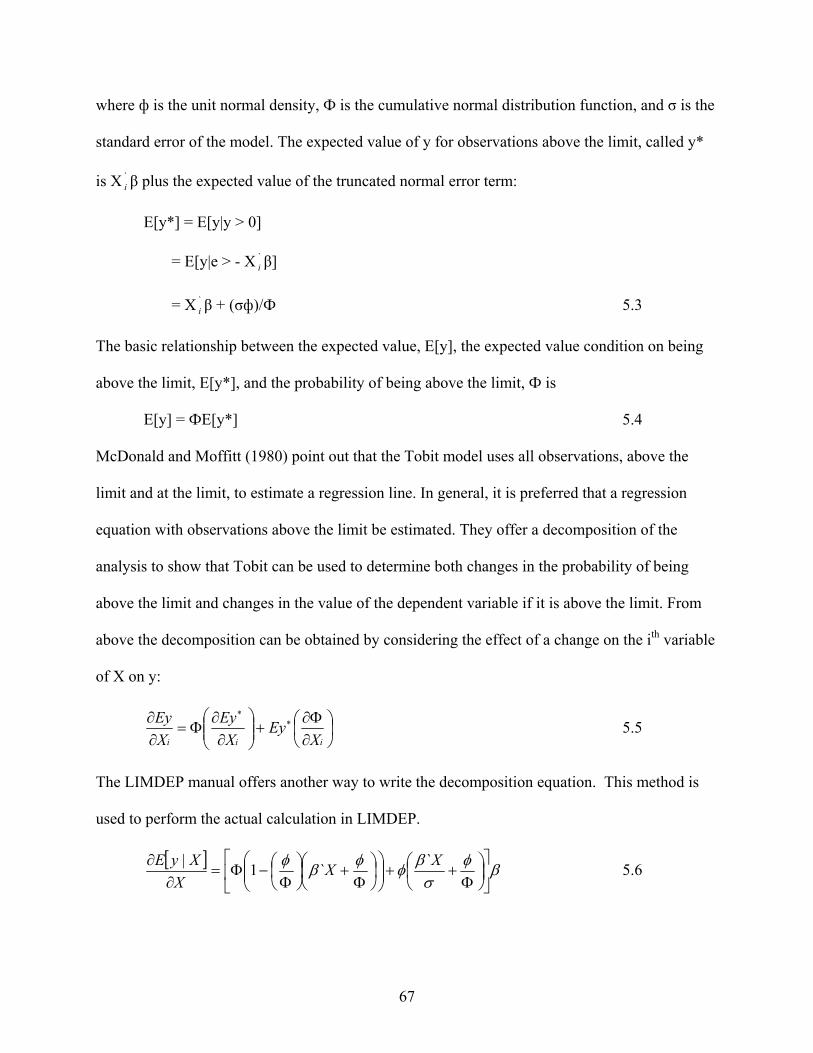
67
where ф is the unit normal density, Ф is the cumulative normal distribution function, and σ is the
standard error of the model. The expected value of y for observations above the limit, called y*
is X `i β plus the expected value of the truncated normal error term:
E[y*] = E[y|y > 0]
= E[y|e > - X `i β]
= X `i β + (σф)/Ф 5.3
The basic relationship between the expected value, E[y], the expected value condition on being
above the limit, E[y*], and the probability of being above the limit, Ф is
E[y] = ФE[y*] 5.4
McDonald and Moffitt (1980) point out that the Tobit model uses all observations, above the
limit and at the limit, to estimate a regression line. In general, it is preferred that a regression
equation with observations above the limit be estimated. They offer a decomposition of the
analysis to show that Tobit can be used to determine both changes in the probability of being
above the limit and changes in the value of the dependent variable if it is above the limit. From
above the decomposition can be obtained by considering the effect of a change on the ith variable
of X on y:
⎟⎠⎞
⎜⎝⎛∂Φ∂
+⎟⎟⎠
⎞⎜⎜⎝
⎛∂∂
Φ=∂∂ ∗
∗
iii XEy
XEy
XEy 5.5
The LIMDEP manual offers another way to write the decomposition equation. This method is
used to perform the actual calculation in LIMDEP.
[ ] βφσβφφβφ
⎥⎦
⎤⎢⎣
⎡⎟⎠⎞
⎜⎝⎛
Φ++⎟⎟
⎠
⎞⎜⎜⎝
⎛⎟⎠⎞
⎜⎝⎛
Φ+⎟
⎠⎞
⎜⎝⎛Φ
−Φ=∂
∂ XXX
XyE ``1| 5.6

68
The total change in y can be broken into two parts, the change in y of those observations above
the limit, weighted by the probability of being above the limit, in this case zero; and the change
in the probability of being above the limit, weighted by the expected value of y if above the limit
(McDonald and Moffitt, 1980).
With both market participation and consumption levels determined by the same equation,
zero consumption observations in the Tobit model are assumed to result from a corner solution to
the utility maximization problem. These zero observations may occur because pecan prices are
too high or other factors that limit market participation such as supply constraints, high
transaction costs, or consumer characteristics, and seasonality of product (Fuller et al, 2004).
Recall in Chapter 3 that we defined willingness to pay by the equality of indirect utility functions
and can be represented in terms of WTP:
U((I - WTP), S1, D) = U(I, S0, D) 5.7
where U represents the indirect utility function, I is income, D represents a set of demographic
and socioeconomic characteristics, and S1 and S0 indicate pecans purchased in the last 24 months
or not. In the case of the dichotomous (yes or no) response question, WTP is not directly
observable. Let z be the observable portion of the indirect utility function U. An individual will
responsd “yes” to the random bid if:
z(( I - Bid), S1, D) + e1 ≥ z(I, S0, D) + e0 5.8
Where e1 and e0 are identically and independently distributed random variables with zero means.
The above equation can be rewritten by specifying z as the functional form of a statistical model,
α1 + β(I - Bid) +e1 ≥ α0 + β*I + e0 5.9
where α1, α0, and β are functions of D. Therefore,
PR(‘yes’) = Pr(α1 + β(I - Bid) + e1 ≥ α0 + β*I + e0) 5.10

69
= Pr(e0- e1 ≤ α1 - α0 – β*Bid) 5.11
= Pr(e ≤ α1- α0 – β*Bid) where e = e0- e1 is the error term.
The Tobit formulation in the study is as follows:
WTPi = WTP *i if WTP *
i < Bidi
= Bidi if WTP *i ≥ Bidi, 5.12
where WTPi is the stated WTP of respondent i and WTP *i is the corresponding latent variable
that is observed for values less than Bidi and is censored for values greater than or equal to Bidi.
The estimation of the Tobit model assumes that the errors are normal and homoscedastic (Long,
1997).
According to demand theory, factors that determine demand are income, own product
price, prices of related goods (substitutes and complements), and tastes and preferences. The
regressors that were chosen for this model theoretically should demonstrate these variables by
displaying a significant level of decision–making power for the respondent to accept or reject the
bid amount. The functional relationship for the willingness to pay curve is expressed as:
WTPi = β0 + β1INC + β2AGE + β3FEMALE + β4KIDS + β5WHITE + β6REGION +
β7EXPENSIVE + β8HIGH_FAT + β9TASTE + β10FAVENUT
+ β11LTP_ANY + β12NUTSPAST + µ 5.13
where:
WTPi = survey respondent’s willingness to pay (in dollars)
INC= household income level (in 1000’s of dollars)
AGE= respondent’s age in years
FEMALE= gender of respondent
(1 = Female, 0= Male)
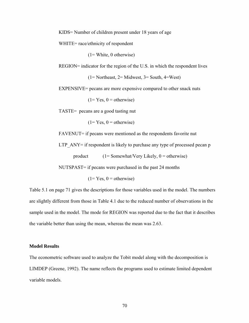
70
KIDS= Number of children present under 18 years of age
WHITE= race/ethnicity of respondent
(1= White, 0 otherwise)
REGION= indicator for the region of the U.S. in which the respondent lives
(1= Northeast, 2= Midwest, 3= South, 4=West)
EXPENSIVE= pecans are more expensive compared to other snack nuts
(1= Yes, 0 = otherwise)
TASTE= pecans are a good tasting nut
(1= Yes, 0 = otherwise)
FAVENUT= if pecans were mentioned as the respondents favorite nut
LTP_ANY= if respondent is likely to purchase any type of processed pecan p
product (1= Somewhat/Very Likely, 0 = otherwise)
NUTSPAST= if pecans were purchased in the past 24 months
(1= Yes, 0 = otherwise)
Table 5.1 on page 71 gives the descriptions for those variables used in the model. The numbers
are slightly different from those in Table 4.1 due to the reduced number of observations in the
sample used in the model. The mode for REGION was reported due to the fact that it describes
the variable better than using the mean, whereas the mean was 2.63.
Model Results
The econometric software used to analyze the Tobit model along with the decomposition is
LIMDEP (Greene, 1992). The name reflects the programs used to estimate limited dependent
variable models.

71
Greene (1992) designed the software, LIMDEP, to be flexible for estimating regression models
most frequently analyzed with cross section data.
After running the model, it was suspected that heteroscedasticity may be present. Recall
that the Tobit assumes the error terms to be normal and homoscedastic. With heteroscedasticity,
the variances among observations are not the same. This means the specific ∧
β is no longer the
Best Linear Unbiased Estimator or BLUE. It remains unbiased and consistent; however the
Table 5.1 Variable Descriptions for Tobit Model
Variable Description Mean Standard Deviation
Income Household Income (divided by 1,000) 60.772 32.606
Age Age of Respondent 48.43 14.229
Female =1 if Female, 0 Male 0.73 0.444
Kids Number of children living in household 0.91 1.241
White =1 if White, 0 otherwise 0.80 0.401
Region Respondent’s geographic location, 1= Northeast, 2= Midwest, 3= South, 4=West
2.48 0.948
Expensive =1 if the price of nuts is expensive relative to other snacks, 0 otherwise 0.91 0.293
High_Fat =1 if respondent strongly agrees or agrees that pecans have a high fat content, 0 otherwise
0.76 0.429
Taste =1 if the respondent strongly agrees or agrees that pecans are a good tasting nut, 0 otherwise
0.97 0.178
Favenut =1 if respondent’s first choice to their favorite nut was pecans, 0 otherwise 0.50 0.501
LTP_Any =1 if respondent is very likely or likely to purchase one or more varieties of new snack pecan product, 0 otherwise
0.31 0.465
Nutspast =1 if pecans were purchased in the last 24 months, 0 otherwise 0.62 0.485
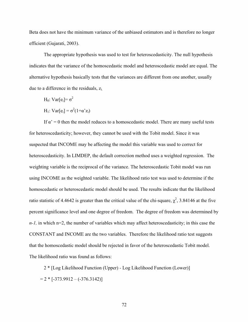
72
Beta does not have the minimum variance of the unbiased estimators and is therefore no longer
efficient (Gujarati, 2003).
The appropriate hypothesis was used to test for heteroscedasticity. The null hypothesis
indicates that the variance of the homoscedastic model and heteroscedastic model are equal. The
alternative hypothesis basically tests that the variances are different from one another, usually
due to a difference in the residuals, zi.
H0: Var[ei]= σ2
H1: Var[ei] = σ2(1+α’zi)
If α’ = 0 then the model reduces to a homoscedastic model. There are many useful tests
for heteroscedasticity; however, they cannot be used with the Tobit model. Since it was
suspected that INCOME may be affecting the model this variable was used to correct for
heteroscedasticity. In LIMDEP, the default correction method uses a weighted regression. The
weighting variable is the reciprocal of the variance. The heteroscedastic Tobit model was run
using INCOME as the weighted variable. The likelihood ratio test was used to determine if the
homoscedastic or heteroscedastic model should be used. The results indicate that the likelihood
ratio statistic of 4.4642 is greater than the critical value of the chi-square, χ2, 3.84146 at the five
percent significance level and one degree of freedom. The degree of freedom was determined by
n-1, in which n=2, the number of variables which may affect heteroscedasticity; in this case the
CONSTANT and INCOME are the two variables. Therefore the likelihood ratio test suggests
that the homoscedastic model should be rejected in favor of the heteroscedastic Tobit model.
The likelihood ratio was found as follows:
2 * [Log Likelihood Function (Upper) - Log Likelihood Function (Lower)]
= 2 * [-373.9912 – (-376.3142)]
73
= 4.6462
The results of the heteroscedastic model are similar to those of the homoscedastic model.
All the signs are consistent and the estimated coefficients are similar between the two models.
Most importantly, the results suggest that the heteroscedastic estimator is more efficient than the
homoscedastic estimator. The majority of the t-values associated with coefficients in the
heteroscedastic model are greater than those in the homoscedastic model. For a comparison
between the homoscedastic and heteroscedastic model, please refer to Appendix B.
Table 5.2 on page 74 provides the estimated coefficients, t-statistic, and p-values from the
effects of the heteroscedastic Tobit model. For the demand equation, coefficients associated with
FAVENUT and FEMALE are significantly different from zero at the ten percent level.
Coefficients associated with AGE, EXPENSIVE, and HIGH_FAT are all significant from zero at
the five percent level. Only one variable is significant at the one percent level and that is
LTP_ANY. The estimated heteroscedastic Tobit model is as follows
WTP = 0.2180 + 0.0013(INCOME) – 0.0072(AGE) + 0.1701(FEMALE)
– 0.0346(KIDS) – 0.0851(WHITE) – 0.0176(REGION)
+ 0.2189(EXPENSIVE) – 0.2067(HIGH_FAT) + 0.2747(TASTE)
+ 0.2020(FAVENUT) + 0.6785(LTP_ANY) – 0.1466(NUTSPAST)
= 0.8908
The mean willingness to pay for a 2.5 ounce single serving snack size bag of pecans is
$0.89 when evaluated at the variables’ mean. This amount was computed by the Tobit regression
and is similar to the mean of the dependent variable WTP which is $0.93. The difference
between the two numbers is due to rounding during the regression. The mean WTP is much

74
lower than the expected WTP, $1.23. The expected WTP was found by taking the mean of those
respondents with bids greater than zero.
As expected, the sign associated with those who believe that pecans are high in fat is
negative; the results suggest that respondent’s who find pecans to be higher in fat are willing to
pay less for a snack size bag of pecans. Although the sign associated with the household income
was positive as expected due to pecans being a normal good, the results suggest that the impact
Table 5.2 Regression Results for the Tobit Model for a Single Serving Snack Size Bag of Pecans
Variable Heteroscedastic Model P-value
Constant 0.2180 (0.702) 0.4824
INC 0.0012 (0.864) 0.3878
Age -0.0072** (-2.114) 0.0345
Female 0.1701* (1.757) 0.0789
Kids -0.0346 (-0.856) 0.3923
White -0.0851 (-0.760) 0.4473
Region -0.1759 (-0.394) 0.6935
Expensive 0.2189** (2.281) 0.0225
High_Fat -0.2067** (-2.172) 0.0298
Taste 0.2778 (1.357) 0.1747
Favenut 0.2020* (1.832) 0.0670
LTP_Any 0.6785*** (4.774) 0.0000
Nutspast -0.1466 (-1.536) 0.1246
*** Indicates significance at the 0.01 level ** Indicates significance at the 0.05 level * Indicates significance at the 0.10 level a Values in parentheses are the t-statsitc for each coefficient

75
of income on willingness to pay was not statistically significant. It is surprising that income did
not play a significant role in this study. Similarly the results indicate that the number of children
under the age of 18 in the household, the region the households are located, and race of the
respondent do not have any significant impact on the willingness to pay for a single serving
snack size bag of pecans.
The model results indicate that females are more willing to pay for a single serving snack
size bag of pecans. As the number of females indicating they would pay for the snack bag of
pecans increases the mean willingness to pay increases by 0.1701. Another significant variable is
AGE. As the age of the respondent increases, the willingness to pay decreases by .0072. The
variable LTP_ANY is significant at the one percent level. As more respondents are likely to
purchase any variety of pecan snack product, the willingness to pay increases by .6785. Again
the varieties of pecan snacks offered to the respondents were raw, sugar and spice, flavored,
roasted, spicy, and salted. The variable EXPENSIVE is significant at the five percent level,
though the sign on the coefficient is somewhat unexpected. One would assume if a person finds
nuts to be more expensive than other snacks, their willingness to pay for pecans snacks would
decrease. However, the sign on this variable’s coefficient is positive indicating that they would
pay more for a snack size bag of pecans.
Two more variables, FAVENUT and NUTSPAST, were thought to have a significant
impact on a person’s WTP for a pecan snack product. From the results it can be seen that only
FAVENUT had any significant effect. Therefore, if a person chose pecans as his or her favorite
snack nut, he or she would be willing to pay more for a pecan snack product. The sign on
NUTSPAST is opposite of what one may have expected to find, but the variable is found to be
insignificant.

76
It was assumed that the more people found pecans to be a good tasting nut, the more they
would be willing to pay for a single serving snack size bag of pecans. However, the variable did
not turn out to have a significant impact on the willingness to pay for the snack pack.
The regression parameters in Table 5.2 cannot be directly interpreted in the same manner
as those obtained from OLS. It is the case that the expected value of y is no longer Xβ as in the
case of OLS regression. To assess the marginal effects of the independent variables on the
dependent variable, WTP, the partial derivatives of Equation 5.5 must be evaluated. The
magnitudes not only depend on whether on the level that the dependent variable is greater than
zero but also the probability that it is greater than zero. The effect of a given change of an
independent variable on the willingness to pay for a single serving snack size bag of pecans is
affected by both the level of positive bids and the probability that the bid levels are greater than
zero, or the probability of market entry.
The elasticities for each variable are computed for the heteroscedastic Tobit model and
presented in Table 5.3 on page 77. The elasticities are decomposed into two components
representing the conditional and market entry elasticities. This is the McDonald and Moffitt
Decomposition discussed earlier in this chapter. The conditional elasticity indicates the change
in conditional expected value given that the probability of purchasing a pecan snack product is
positive. The market entry elasticity indicates the change in probability of purchasing a pecan
snack product given that the conditional expected value is positive. In general, the
decomposition disaggregates Tobit effects into (1) effects on the probability of being above zero
and (2) effects conditional upon being above zero.

77
The results shown in Table 5.3 suggest that the conditional elasticity and the market entry
elasticity equally account for the effect of change in socioeconomic and consumer characteristics
on the willingness to pay for a snack size bag of pecans. The elasticities describe the percent
change in each variable as it relates to the level or probability of the WTP. A one percent
increase in age will result in a .25 percent decrease in the probability of market entry. The level
of WTP is affected by the positive amounts. Another way to look at these elasticities is that if
there is an increase in age, then 0.25 percent of the population will drop out of the market
completely. The variable that has the highest effect on market entry is FEMALE followed by
TASTE, though TASTE was found to be insignificant.
Table 5.3 Estimated Elasticitiesa of the Heteroscedastic Tobit Model Variable Total Conditional Market Entry
Constant 0.1743 0.0876 0.0867 Inc_000 0.0604 0.0304 0.0300 Age -0.0052 -0.0026 -0.0025 Femaleb 6.5774 3.3136 3.2638 Kids -0.0201 -0.0101 -0.0100 Whiteb -0.0543 -0.0273 -0.0270 Region -0.0355 -0.0176 -0.0174 Expensiveb 0.1585 0.0797 0.0787 High_Fatb -0.1252 -0.0629 -0.0622 Tasteb 0.2125 0.1069 0.1056 Favenutb 0.0802 0.0403 0.0399 LTP_Anyb 0.1701 0.0855 0.0845 Nutspastb -0.0731 -0.0368 -0.0363 a Elasticities calculated at the mean level b Due to binary responses, percent changes do not have the same meaning
78
Chapter 6
Summary and Conclusions
Conclusions
Pecan production occurs in the Southeastern and Southwestern United States down
through the northern Mexican states. The majority of pecans are grown in Georgia while Texas
actually has more pecan trees. Georgia pecan trees tend to be older and have been in production
for many years, while other states have newer, younger trees which may take longer to provide
higher volumes. As consumption increases, imports have been slowly increasing. The U.S.
imports high quality pecans from Mexico to supplement low production years. Also, exports
have been slowly increasing in the past few years due to increased overseas consumption China
looks to be an up and coming important importer.
Since pecans have an alternate bearing pattern which yields greater quantities of pecans
one year with a lower quantity the following year, storage becomes an important issue for
growers and shellers. The variation in production leads to variation of prices from year to year
which often makes it difficult for producers, shellers, and wholesalers to market their crop
without storage. New technologies in storage that would decrease costs of storage and improve
the quality could help the industry be more profitable and could also lead to the opportunity to
market a snack product more easily.
Currently pecans tend to be a seasonal item purchases widely during the November
through January holidays. The Georgia Pecan Growers Association consists of pecan growers
throughout the state of Georgia who are trying to find new ways to market pecans and increase
79
the demand throughout the year. One option examined is to create a snack size bag of pecans
that one may find in the snack aisle at the local grocery or conveniences store or even the gas
station.
In this study, phone survey results about consumers’ purchasing behaviors, preferences,
and attitudes towards pecans were analyzed using simple statistical procedures and regression
analysis. The survey was conducted on a national level in hopes of providing a national
representation of pecan consumers. The first objective was to determine from the survey,
current consumption patterns and the demographic makeup of the potential snack pecan
consumer. Currently the majority of pecan consumption occurs during November through early
March and is when pecans are available fresh. Almost one-third of the respondents who
indicated purchasing pecans in the past 24 months live in the Southern portion of the United
States. The survey results show that out of the pecan consumer survey, 16.8 percent eat pecans
more than once a week as a snack. In addition, a little less than half of the survey respondents
have purchased pecans as a snack.
The survey results also show that the average pecan consumer does not purchase them
very often, fewer than three times a year, with most purchasing one pound bags of halves. A six
month average of the dollar amount spent on pecans is $36.37.
Early in the survey, consumers were asked if they had purchased pecans in the past 24
months. The complete survey was not administered for those consumers who answered ‘no’ to
this question. However, they were then asked one additional question, “Why have you not
purchased pecans in the past 24 months?” There were several major reasons consumers gave for
not purchasing pecans. Over 50 percent indicated they do not consume pecans because they do
not like the taste of them. Other reasons included, owning a pecan tree or have friends that own

80
a tree, have an allergy or some other medical reason, not readily available to them, or they
consider pecans too expensive. Some respondents were categorized as ‘other’ which contained
reasons such as they may purchase pecans for baking but have not done so in the last 24 months
and just do not purchase them.
The second objective in this study was to determine the demographic profile of a pecan
snack consumer. The demographic profile of a pecan snack consumer can be determined by
analyzing the responses that are specific to a pecan consumer who indicated they eat pecans as a
snack once a month or more. The results indicate that the household income of a pecan snack
consumer is considerably higher than that of the average American. Also, those consumers
earning more than $105,000 annually are more likely to purchase pecans as a snack. Forty-five
percent of those respondents have obtained a bachelor’s degree or higher as compared to 31
percent for the national average. Seventy-two percent of the respondents who indicated they
purchase pecans as a snack once a month or more were female, which is much greater than the
U.S. female population average of 51 percent. The median age of the typical pecan snack
consumer is 52 years of age compared to the U.S. median age of 35 years. The results seem to
indicate that that the average pecan snack consumer would be older, more affluent and educated.
It would be appropriate for the pecan industry to focus on marketing strategies to younger
consumers to increase the demand for pecans. Also, pecan snacks need to be heavily marketed
and promoted in the Northeast and Western U.S. as they are less likely than Southerners to eat
pecans on a regular basis.
Statistical analysis revealed that the majority of pecan consumers purchase their pecans at
the grocery store. This has implications when the industry begins to focus on where to market the
snack products. The next largest percentage of places where people purchase pecans was the

81
‘other’ category. There were more responses for the category ‘other’ than for roadside stand,
fundraiser, catalog orders, or specialty.
The mean willingness to pay was calculated for several categories such as income level,
region, where pecans are purchased, and bag size most often purchased to determine if there are
differences among these characteristics. When comparing across income levels, the mean WTP
was found to be similar in all categories. The mean WTP was consistent across regions in the
Untied States. However, those living in the Northeast and the South have a slightly higher mean
WTP than those in the Midwest and West.
Using cross-tabular analysis, those living in the Northeast and having the lowest level of
income are willing to pay the most ($1.30) for a pecan snack product. Additionally, those living
in the South with the same level of income are willing to pay the least ($0.80) for the
hypothetical product. At the income level of $49,999.50, the West is willing to pay the least
($0.76), while the other three regions are all willing to pay over $0.90 per pack.
Consumers were also questioned about their likelihood to purchase different varieties of
pecan snack products. From the results it appears that roasted pecans have the potential to be a
successful product with the majority of the people stating that they would be likely to purchase
the product. This was consistent across all regions of the U.S. Over 50 percent of the consumers
questioned stated that they were somewhat or very likely to purchase a raw pecan snack product.
The South had the highest percentage at 63 percent. Although the percentage did not change
across regions, the South had the highest percentage of likeliness to purchase a raw pecans snack
product.
A glazed pecan snack product had around 50 percent of consumer responding that they
would be somewhat or very likely to purchase. The Northeast had the highest percent of very
82
likely responses for this product with 29 percent, which was much higher than the Midwest 20
percent. The only variety of pecan snack product, with an overwhelming response of unlikely or
very unlikely to purchase was spicy. Seventy-eight percent of those in the Midwest stated that
they were unlikely or very unlikely to purchase a spicy pecan snack product. Northeasterners
had the highest percentages of somewhat or very likely to purchase with 37 percent.
The third objective of the study was to determine consumers’ mean willingness to pay for
a 2.5 ounce single serving snack size bag of pecans using the data from the survey analysis. The
Tobit procedure was used to determine the mean WTP for a 2.5 ounce snack size bag of pecans.
From the Tobit model, the mean WTP was estimated to be $0.89 per 2.5 ounce single serving
snack size bag of pecans. This price is less than the expected WTP, $1.23.
The results of the survey analysis may provide a start to developing a marketing plan for
pecan products. Pecan producers and processors need to be able to increase the frequency of
pecan purchases, leading to an increase in overall demand. By directing efforts toward
marketing to people more likely to purchase pecans; their time and capital may be better spent.
This analysis can provide producers with a product price which will be useful in determining the
feasibility for new snack product markets.
Limitations and Future Research
Though the phone survey results provided a pecan consumer profile and a WTP, test
marketing may be more suitable to determine the actual willingness to pay for a pecan snack
product. Providing a consumer with the actual product should enhance the quality of the results.
Combining a supermarket situation with a taste test will also provide more insight as to how
much a person would be willing to pay for a single serving snack size bag of pecans. In this
83
study, the consumer is not actually in the position to purchase the product which therefore may
inflate their stated willingness to pay.
Since the mean WTP was estimated to be a relatively low price of $0.89, additional
research could be conducted to determine what consumers are actually willing to pay if interest
is present for such products. It is uncertain that the pecan industry will benefit from producing
and marketing this pecan snack product at a price this low. By producing the product and
performing a test market, the willingness to pay can be better observed through actual purchases.
However, this does require a pecan processor to create the single serving snack size bag of
pecans. Having the option to purchase the actual product in a market setting may give more
realistic prices than from the survey. The surveyors could also set up a taste panel and test which
flavors or forms of pecans are preferred. One additional option would be place the product on
store shelves and monitor purchases through these stores with the pecans being sold at different
price levels. This will allow one to observe quantities and frequencies of the pecan snack
products purchased. The industry may want to start their test marketing of a pecan snack
product, focusing on those groups who have the highest mean WTP such as the group of
participants with an income level of $17,499.49 and residing in the Northeast ($1.30).
However, if a follow-up survey were conducted instead or addition to the test marketing,
it should include a price-quantity question. The particular question could ask the respondent
how much of the snack pecan product they would be willing to purchase at their stated price.
This would allow for a hypothetical demand curve to be formatted. Such a survey could also be
phrased to determine how many times a week/month would one purchase a snack size bag of
pecans.
84
REFERENCES
Allen, Christopher. Measuring Values for Wetlands Protection in a Developing Country from Domestic and International Citizen Groups. Master’s Thesis, University of Georgia, Dept. of Agricultural and Applied Economics. 2004.
Blend, Jeffrey R. and Eileen O. van Ravenswaay. “Measuring Consumer Demand for Ecolabeled
Apples.” American Journal of Agriclutral Economics. 81(5): 1072-1077, 1999. Boccaletti, Stefano and Michele Nardella. “Consumer Willingness to Pay for Pesticide-Free
Fresh Fruit and Vegetables in Italy.” International Food and Agribusiness Management Review. Vol 3. p.297-310, 2001.
Buzby, Jean C., John A. Fox, Richard C. Ready, and Stephen R. Crutchfield. “Measuring
Consumer Benefits of Food Safety Risk Reductions.” Journal of Agricultural and Applied Economics. 30(1): 69-82, 1998.
Champ, Patricia A, Kevin J. Boyle, and Thomas C. Brown. A Primer on Non-Market Valuation.
Kluwer Academic Publishers, 2003. Dasgupta, Siddhartha, John Foltz, and Bonnie Jacobsen. “Trout Steaks: Consumer Perceptions of
a New Food Item.” Journal of Food Distribution. 31(3):37-48, November 2000. Field, Barry C. Environmental Economics: An Introduction. McGraw-Hill, Inc, 1994. Fleisher, Belton M., Edward J Ray, and Thomas J. Kneisner. Principles of Economics. Wm. C.
Brown. 1987. Freeman III, A. Myrick. The Measurement of Environmental and Resource Values. Resources
for the Future, Washington D.C. 2003. Fuller, Frank H., John C. Beghin, and Scott Rozelle. “Urban Demand for Dairy Products in
China: Evidence from New Survey Data.” Working Paper 04-WP 380. Iowa State University, 2004.
Giraud, Kelly, John Loomis, and Richard Johnson. “Two Valuation Questions in One Survey: Is
it a Recipe for Sequencing and Instrument Context Effects.” Applied Economics. 31:957-964, 1999.
Green, William H. LIMDEP: User’s Manual and Reference Guide. Version 6.0. Econometric
Software, Inc, 1992. Govindasamy, Ramu and John Italia. “A WIllingess-to-Purchase Comparison of Integrated Pest
Management and Conventional Produce.” Agribusiness. 14(5):403-414, 1998.
85
Gujarati, Damodar N. Basic Econometrics. Fourth Edition. McGraw Hill, 2003. Hall, Charles R., Carl E. Shafer, Lance D. Pate, and Corey S. Anderson. Characteristics and
Marketing Practices of Texas Pecan Shellers. Texas A & M University Faculty Paper Series 98-12, May 1998.
Hanemann, W. Michael. “Willingness to Pay and Willingness to Accept: How Much Can they
Differ?” The American Economic Review. 81(3):635-647, 1991. Heckman, James J. “Sample Selection Bias as a Specification Error.” Econometrica. 47(1):153-
162, 1979. Herriges, Joseph A and Jason F. Shogren. “Starting Point Bias in Dichotomous Choice Valutaion
with Follow-Up Questioning.” Journal of Environmental Economics and Management. 30(8): 112-131, 1996.
Huang, Chung L. “Simultaneous-Equation Model for Estimating Consumer Risk Perceptions,
Attitudes, and Willingness-to-Pay for Residue-Free Produce.” The Journal of Consumer Affairs. 27(2):377-396, 1993.
Hubbard, Eugene E., Joseph C. Purcell, and Stephen L. Ott. “Purchasing and Marketing
Practices of Georgia Pecan Accumulators and Shellers.” The Georgia Agricultural Experiment Station Research Report544, December 1987.
Jekanowski, Mark D., Daniel R. Williams II, and William A. Scheik. “Consumer’s Willingness
to Purchase Locally Produced Agricultural Products: An Analysis of an Indiana Survey.” Agricultural and Resource Economics Review. 29(8): 43-53, April 2000.
Johnson, Doyle C. “Economic Trends in the U.S. Pecan Market with an Overview of The U.S.
and World Tree Nut Complex.” United States Department of Agriculture, Economic Research Service. Fruit and Tree Nuts Outlook Report: Special Article. FTS-282. Washington D.C. March 1998.
Johnston, Jack and John DiNardo. Econometric Methods. McGraw-Hill, 1997. Lillywhite, Jay M., Ereney Hadjigeorgalis, and Esteban Herrera. Marketing Channels for
Pecans. Guide Z-307. Las Cruces, NM: New Mexico State University, Coop. Ext. Ser., 2003.
Long, J.S. Regression Models for Categorical and Limited Dependent Variables. Thousand
Oaks, CA. Sage. 1997
86
Loureiro, Mary J. and Wendy J. Umberger. “Estimating Consumer Willingness-to-Pay for Country-of-Origin Labels for Beef Products.” Paper selected for 2002 American Agricultural Economics Association Annual Meetings, Long Beach, CA July 28-31. 2002.
Loureiro, Maria L., Jill J. McCluskey, and Ron C. Mittelhammer. “Will Consumers Pay a
Premium for Eco-Labeled Apples?” The Journal of Consumer Affairs. 36(2): 203-219, 2002.
Loureiro, Maria L. and Susan Hine. : Discovering Niche Markets: A Comparison of Consumer
Willingness to Pay for a Local(Colorado-Grown), Organic, and GMO-free Product.” Paper selected for the 2001 American Agricultural Economics Association Annual Meeting.
Luck, Jayon L. and Darren Hudson. “Willingness-to-Pay Estimates and Their Relevance to
Agribusiness Decision Making.” Review of Agricultural Economics. 26(2): 152-169, 2004.
McDonald, John F. and Robert A. Moffitt. “The Uses of the Tobit Analysis.” The Review of
Economics and Statistics. 62:318-321, 1980. Misra, Sukant K., Chung L. Huang, and Stephen L. Ott. “Consumer Willingness to Pay for
Pesticide-Free Fresh Produce.” Western Journal of Agricultural Economics. 16(2): 218-227, December 1991.
Mukhopadhaya, Kaushik, Bishwa Adhikari, Gerald Mumma, and Mario Teisl. “Consumer’s
Willingness to Pay for Food Safety: A Pathogen Specific Analysis.” Paper prepared for presentation at the American Agricultural Economics Association Annual Meeting, Denver, CO, August 2004.
National Pecan Growers Association, http:/www.ilovepecans.org/. NIST/SEMATECH e-Handbook of Statistical Methods. “Related Distributions.” 1.3.6.2
http://www.itl.nist.gov/div898/handbook/eda/section3/eda362.htm#CDF /, 2005. Park, John L. and Oral Capps Jr. “Demand for Prepared Meals by US. Households.” American
Journal of Agricultural Economics. 79(3):814-824, 1997. Park, Timothy A., and Wojciech Florkowski. “Demand and Quality Uncertainty in Pecan
Purchasing Decisions.” J. of Agricultural and Applied Economics. 31(1):29-39 April 1999.
Peña, Jose G., Parr Rosson III, and Flynn J. Adcock. U.S. Pecan Imports and Exports and the
Effect on Trade. Texas A & M University, Extension Agricultural Economics Faculty Paper Series. March 6, 2001.

87
Randall, Alan. Resource Economics: an Economic Approach to Natural Resources and Environmental Policy. New York: Wiley. 1987.
Rimal, Arbindra P. and Stanley M. Fletcher. “Snack Peanuts Purchase Pattern: Effects of
Nutritional Considerations and Household Characteristics.” Journal of Agricultural and Applied Economics. 34(1): 51-65, April 2002.
Rosengarten Jr, Frederic. Book of Edible Nuts. Walker Publishing Co, Inc 1984. Sales, Anne E., Mary E. Plomondon, David J. Magid, John A. Spertus, and John S. Rumsfield.
“Assessing Response Bias from Missing Quality of Life Data: The Heckman Method.” Health and Quality of Life Outcomes. Online 2(49), September 16, 2004.
Taylor, Susan. “Pecans in Bakery Foods” National Pecan Shellers Association Technical
Bulletin 23(8) August 2001. Turnbull, Stephen J. “MBA: Microeconomics” Class Lecture Notes.
http://turnbull.sk.tsukuba.ac.jp/Teach/Micro/ohp14.pdf United States Census Bureau. 2000. United States Department of Agriculture, Economic Research Service. Fruit and Tree Nuts
Outlook Report: Commodity Highlight. FTS-304. Washington D.C. May 2003. United States Department of Agriculture, Economic Research Service. Fruit and Tree Nuts
Outlook Report: Commodity Highlight. FTS-2003. Washington D.C. October 2003. United States Department of Agriculture, Economic Research Service. Fruit and Tree Nuts
Outlook Report: Commodity Highlight. FTS-2004. Washington D.C. October 2004 Varian, Hal R. Intermediate Microeconomics: A Modern Approach. W.W> Norton and
Company, New York. 1996. Wagner, Al. “Pecan Storage: An Important Post-Harvest Practice in Preventing Nut Damage.”
Pecan South. p. 40-43 September 1980. Wessells, Cathy R., Robert J. Johnston, and Holger Donath. “Assessing Consumer Preferences
for Ecolabled Seafood: The Influence of Species, Certifier, and Household Attributes.” American Journal of Agricultural Economics. 81(5): 1084-1090, 1999.
Wessells, Cathy R. and Hoan G. Anderson. “Consumer Willingness to Pay for Seafood Safety
Assurances.” Journal of Consumer Affairs. 29(1): 85-108, 1995. Wetzstein, Michael J. Microeconomic Theory. South-Western, 2005.
88
Wood, B.W. “Price: Production Relationship and Production Characteristics of U.S. Pecan Industry.” Proceedings of the 92nd Southeastern Pecan Growers Association Annual Convention, March 14-16, (2000): 117-132.
Woodruff, Jasper Guy. Tree Nuts: Production, Processing, Products. University of Georgia.
1979. www.digitaleconomist.com www.econtools.com http://turnbull.sk.tsukuba.ac.jp/Teach/Micro/ohp14.pdf Yoo, Seung-Hoon, Seung-Jun Kwak, and Tai-Yoo Kim. “Modeling Willingness to Pay for
Responses from Dichotomous Choice Contingent Valuation Surveys with Zero Observations.” Applied Economics. 33(4):523-29, 1998.
89
APPENDICES
Appendix A:
Consumer Pecan Use Survey 2004
CATI Format

90
Consumer Pecan Use Survey 2004
Hi, I’m [NAME] from the University of Georgia Survey Research Center, calling for the UGA Center for Agribusiness and Economic Development. We are conducting a short study of food preferences. Do you have a few minutes right now to answer a few questions? [INTERVIEWER: THE SURVEY SHOULD LAST ABOUT 15 MINUTES] In order for the results of the survey to be representative of the state's population, I need to speak with the youngest male, 18 years of age or older, who lives in the household. Would that be you?
1. Yes [CONTINUE] 2. No [MAY I SPEAK TO THE OLDEST FEMALE 18 OR OLDER?]
[REINTRODUCE YOURSELF AND THE STUDY OR ARRANGE TIME FOR CALL-BACK AND GET THE RESPONDENT'S FIRST NAME]
Thank you. Before we begin, let me assure you that all of the information that you provide will be kept strictly confidential. We are interviewing a number of people like you, and all the information we collect will be combined and reported together. The interview is voluntary, and if you don't want to answer any particular question, just tell me and we'll skip to the next one. Also, my Supervisor may listen to part of the interview for quality control purposes. Thank you for agreeing to complete this survey for the Center for Agribusiness and Economic Development of the University of Georgia Extension Service. Q1. To begin, when you think of snack nuts, what first comes to mind?
[INTERVIEWER NOTE: CHOOSE ALL MENTIONED, PROMPT IF NECESSARY]
[PROGRAMMER NOTE: ORDERED]
1. Almonds 2. Brazil nuts 3. Cashews 4. Hazelnuts 5. Macadamia 6. Peanuts 7. Pecans 8. Pistachios 9. Walnuts 10. Other (please specify):___________________________________ 11. Ref/DK/NA 12. Exit

91
Q2. Thinking about the various snack nuts, which, if any, is your favorite nut? What is your next favorite?
[INTERVIEWER NOTE: CHOOSE ALL MENTIONED, PROMPT IF NECESSARY]
[PROGRAMMER NOTE: ORDERED]
1. Almonds 2. Brazil nuts 3. Cashews 4. Hazelnuts 5. Macadamia 6. Peanuts 7. Pecans 8. Pistachios 9. Walnuts 10. Other (please specify):___________________________________ 11. No favorites 12. Ref/DK/NA 13. Exit
Q3. Which nuts have you purchased in the past 24 months?
[INTERVIEWER NOTE: CHOOSE ALL MENTIONED, PROMPT IF NECESSARY]
[PROGRAMMER NOTE: ORDERED]
1. Almonds 2. Brazil nuts 3. Cashews 4. Hazelnuts 5. Macadamia 6. Peanuts 7. Pecans 8. Pistachios 9. Walnuts 10. Other (please specify):___________________________________ 11. None 12. Ref/DK/NA 13. Exit
[PROGRAMMER NOTE: IF Q3 DOES NOT EQUAL 7, ASK Q4 AND Q5, OTHERWISE SKIP TO Q6] Q4. Have you purchased pecans in the last 24 months?
1. Yes [SKIP TO Q6] 2. No

92
9. Ref/DK/NA
Q5. Why have you not purchased any pecans in the last 24 months?
_____________________________________________________________________
[PROGRAMMER NOTE: END SURVEY AND CODE 1110—COMPLETE, NO PECANS (SAVE DATA)]
Q6. Are you familiar with any of the following nuts?
[INTERVIEWER NOTE: CHOOSE ALL THAT APPLY] [PROGRAMMER NOTE: YES/NO TOGGLE]
1. Almonds 2. Brazil nuts 3. Cashews 4. Hazelnuts 5. Macadamia 6. Peanuts 7. Pecans 8. Pistachios 9. Walnuts 10. Other (please specify):___________________________________ 11. None 12. Ref/DK/NA 13. Exit
Q7 Which snack nuts do you eat most often by themselves? [INTERVIEWER NOTE: CHOOSE ALL THAT APPLY, PROMPT WITH, “WHAT OTHERS?”] [PROGRAMMER NOTE: ORDERED]
1. Almonds 2. Brazil nuts 3. Cashews 4. Hazelnuts 5. Macadamia 6. Peanuts 7. Pecans 8. Pistachios 9. Walnuts
10. Other (please specify):___________________________________

93
11. None 12. Ref/DK/NA 13. Exit
Q8. Please estimate the amount of money you spent on nuts and nut products such as raw nuts for baking, chocolate covered nuts, salted mixes, etc. in the last 6 months.
____________ dollars 999 – Ref/DK/NA [RANGE: 0 – 999] Q9. How many times have you bought pecans since January 1st? __________ times 999 – Ref/DK/NA [RANGE: 0 – 999] [PROGRAMMER NOTE: IF Q9 = 0 OR 999, SKP TO Q13] Q10.1 Did you buy pecans as a gift?
1. Yes 2. No [SKIP TO Q10.3] 9. Ref/DK/NA [SKIP TO Q10.3]
Q10.2 In what form do you generally buy pecans for a gift? [INTERVIEWER NOTE: CHOOSE ALL THAT APPLY] [PROGRAMMER NOTE: YES/NO TOGGLE]
1. In-shell 2. Pecan halves 3. Pecan pieces 4. Do not buy pecans for gifts 5. Ref/DK/NA 6. Exit
Q10.3 Did you buy pecans to eat as a snack?
1. Yes 2. No [SKIP TO Q10.5] 9. Ref/DK/NA [SKIP TO Q10.5]

94
Q10.4 In what form do you generally buy pecans to eat as a snack? [INTERVIEWER NOTE: CHOOSE ALL THAT APPLY] [PROGRAMMER NOTE: YES/NO TOGGLE]
1. In-shell 2. Pecan halves 3. Pecan pieces 4. Do not buy pecans for snacks 5. Ref/DK/NA 6. Exit
Q10.5 Did you buy pecans for cooking or baking?
1. Yes 2. No [SKIP TO Q10.7] 9. Ref/DK/NA [SKIP TO Q10.7]
Q10.6 In what form do you generally buy pecans for cooking or baking? [INTERVIEWER NOTE: CHOOSE ALL THAT APPLY] [PROGRAMMER NOTE: YES/NO TOGGLE]
1. In-shell 2. Pecan halves 3. Pecan pieces 4. Do not buy pecans for cooking or baking 5. Ref/DK/NA 6. Exit
Q10.7 Did you buy pecans for some other reason that we haven’t mentioned? 1. Yes 2. No [SKIP TO Q11a - e] 9. Ref/DK/NA [SKIP TO Q11a - e]
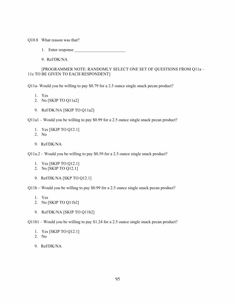
95
Q10.8 What reason was that? 1. Enter response ________________________ 9. Ref/DK/NA
[PROGRAMMER NOTE: RANDOMLY SELECT ONE SET OF QUESTIONS FROM Q11a – 11e TO BE GIVEN TO EACH RESPONDENT]
Q11a- Would you be willing to pay $0.79 for a 2.5 ounce single snack pecan product?
1. Yes 2. No [SKIP TO Q11a2] 9. Ref/DK/NA [SKIP TO Q11a2]
Q11a1 – Would you be willing to pay $0.99 for a 2.5 ounce single snack pecan product?
1. Yes [SKIP TO Q12.1] 2. No 9. Ref/DK/NA
Q11a.2 – Would you be willing to pay $0.59 for a 2.5 ounce single snack product?
1. Yes [SKIP TO Q12.1] 2. No [SKIP TO Q12.1] 9. Ref/DK/NA [SKP TO Q12.1]
Q11b – Would you be willing to pay $0.99 for a 2.5 ounce single snack pecan product?
1. Yes 2. No [SKIP TO Q11b2] 9. Ref/DK/NA [SKIP TO Q11b2]
Q11b1 – Would you be willing to pay $1.24 for a 2.5 ounce single snack pecan product?
1. Yes [SKIP TO Q12.1] 2. No 9. Ref/DK/NA

96
Q11b2 – Would you be willing to pay $0.74 for a 2.5 ounce single snack pecan product?
1. Yes [SKIP TO Q12.1] 2. No [SKIP TO Q12.1] 9. Ref/DK/NA [SKIP TO Q12.1]
Q11c – Would you be willing to pay $1.19 for a 2.5 ounce single snack pecan product?
1. Yes 2. No [SKIP TO Q11c2] 9. Ref/DK/NA [SKIP TO Q11c2]
Q11c1 – Would you be willing to pay $1.48 for a 2.5 ounce single snack pecan product?
1. Yes [SKIP TO Q12.1] 2. No 9. Ref/DK/NA
Q11c2 – Would you be willing to pay $0.89 for a 2.5 ounce single snack pecan product?
1. Yes [SKIP TO Q12.1] 2. No [SKIP TO Q12.1] 9. Ref/DK/NA [SKIP TO Q12.1]
Q11d – Would you be willing to pay $1.39 for a 2.5 ounce single snack pecan product?
1. Yes 2. No [SKIP TO Q11d2] 9. Ref/DK/NA [SKIP TO Q11d2]
Q11d1 – Would you be willing to pay $1.73 for a 2.5 ounce single snack pecan product?
1. Yes [SKIP TO Q12.1] 2. No 9. Ref/DK/NA
Q11d2 – Would you be willing to pay $1.04 for a 2.5 ounce single snack pecan product?
1. Yes [SKIP TO Q12.1] 2. No[SKIP TO Q12.1] 9. Ref/DK/NA [SKIP TO Q12.1]
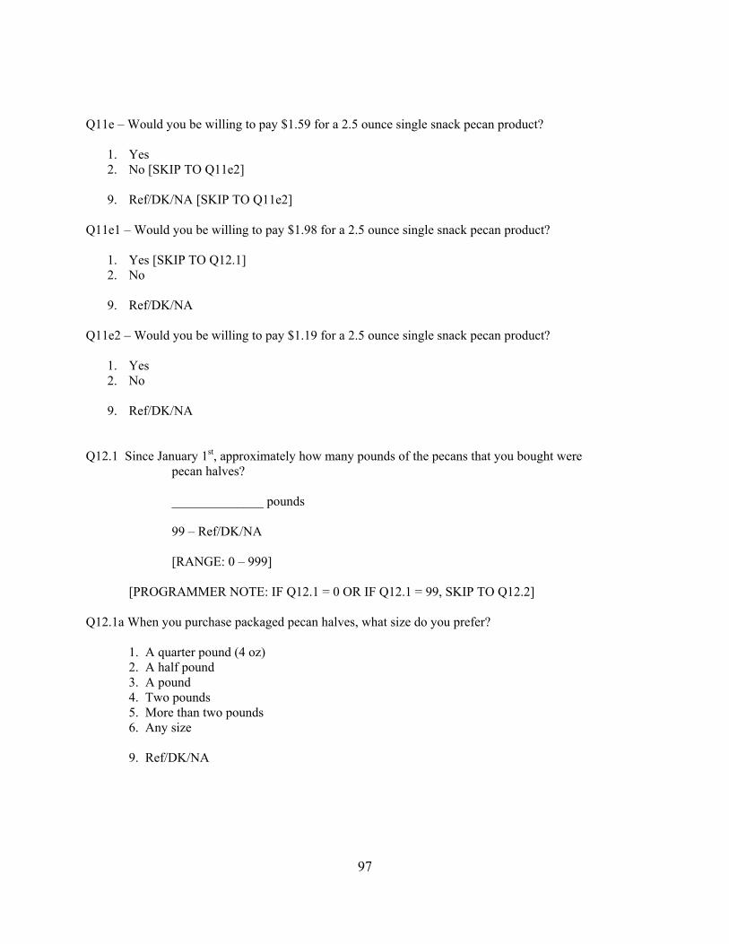
97
Q11e – Would you be willing to pay $1.59 for a 2.5 ounce single snack pecan product?
1. Yes 2. No [SKIP TO Q11e2] 9. Ref/DK/NA [SKIP TO Q11e2]
Q11e1 – Would you be willing to pay $1.98 for a 2.5 ounce single snack pecan product?
1. Yes [SKIP TO Q12.1] 2. No 9. Ref/DK/NA
Q11e2 – Would you be willing to pay $1.19 for a 2.5 ounce single snack pecan product?
1. Yes 2. No 9. Ref/DK/NA
Q12.1 Since January 1st, approximately how many pounds of the pecans that you bought were pecan halves?
______________ pounds 99 – Ref/DK/NA [RANGE: 0 – 999]
[PROGRAMMER NOTE: IF Q12.1 = 0 OR IF Q12.1 = 99, SKIP TO Q12.2] Q12.1a When you purchase packaged pecan halves, what size do you prefer? 1. A quarter pound (4 oz) 2. A half pound 3. A pound 4. Two pounds 5. More than two pounds 6. Any size 9. Ref/DK/NA

98
Q12.1b Typically, how much do you pay per pound for pecan halves? [INTERVIEWER NOTE: ENTER EXACT AMOUNT] _____________ dollars 99.99 – Ref/DK/NA [RANGE: 00.00 – 99.99] Q12.1c. How do you store your pecan halves? [INTERVIEWER NOTE: CHOOSE ALL THAT APPLY] [PROGRAMMER NOTE: ORDERED] 1. Store them in the refrigerator 2. Keep them in the pantry 3. Store them in the freezer 4. Keep them on the counter
5. Other (Specify)________________________________ 6. Ref/DK/NA 7. Exit Q12.2 Since January 1st, approximately how many pounds of the pecans that you bought were pecan
pieces?
_____________ pounds 99 – Ref/DK/NA [RANGE: 0 – 99]
[PROGRAMMER NOTE: IF Q12.2 = 0 OR IF Q12.2 = 99, SKIP TO Q12.3] Q12.2a When you purchase packaged pecan pieces, what size do you prefer? 1. A quarter pound (4 oz) 2. A half pound 3. A pound 4. Two pounds 5. More than two pounds 6. Any size 9. Ref/DK/NA

99
Q12.2b Typically, how much do you pay per pound for pecan pieces?
[INTERVIEWER NOTE: ENTER EXACT PRICE. PECAN PIECES ON OVERAGE COST $7.29 PER POUND]
_____________ dollars 99.99 – Ref/DK/NA [RANGE: 00.00 – 99.99] Q12.2c. How do you store your pecan pieces? [INTERVIEWER NOTE: CHOOSE ALL THAT APPLY] [PROGRAMMER NOTE: ORDERED] 1. Store them in the refrigerator 2. Keep them in the pantry 3. Store them in the freezer 4. Keep them on the counter
5. Other (Specify)________________________________ 6. Ref/DK/NA 7. Exit [PROGRAMMER NOTE: PECAN MEAL AND PECAN GRANULE QUESTIONS WERE DELETED] Q12.3 Since Jaunary 1st, how many pounds that you bought were in-shell pecans?
________________pounds 99 – Ref/DK/NA [RANGE: 0 – 99] [PROGRAMMER NOTE: IF Q12.3 = 0 OR IF Q12.3 = 99, SKIP TO Q13] Q12.3a When you purchase packaged in-shell pecans, what size do you prefer? 1. A quarter pound (4 oz) 2. A half pound 3. A pound 4. Two pounds 5. More than two pounds 6. Any size 9. Ref/DK/NA

100
Q12.3b Typically, how much do you pay per pound for in-shell pecans?
[INTERVIEWER NOTE: ENTER EXACT PRICE. IN-SHELL PECANS ON AVERAGE COST ABOUT $4.00 PER POUND]
_____________ dollars 99.99 – Ref/DK/NA [RANGE: 00.00 – 99.99] Q12.3c. How do you store your in-shell pecans? [INTERVIEWER NOTE: CHOOSE ALL THAT APPLY] [PROGRAMMER NOTE: ORDERED] 1. Store them in the refrigerator 2. Keep them in the pantry 3. Store them in the freezer 4. Keep them on the counter
5. Other (Specify)________________________________ 6. Ref/DK/NA 7. Exit Q13. Where do you generally purchase your pecans? [INTERVIEWER NOTE: CHOOSE ALL THAT APPLY, PROMPT WITH, “WHERE ELSE?”] [PROGRAMMER NOTE: ORDERED]
1. Grocery Store 2. Internet Order 3. Catalog Order 4. Specialty Store 5. Through a fund raiser 6. Road side stand 7. Other (Please specify) _________________ 8. Ref/DK/NA 9. Exit

101
Q14. How often do you typically purchase pecans? [INTERVIEWER NOTE: CHOOSE ALL THAT APPLY, PROMPT WITH, “ANY OTHER TIMES?”] [PROGRAMMER NOTE: ORDERED]
1. On a regular basis 2. Only during harvest 3. Only during holidays (Which ones?) __________________________ 4. On special occasions other than holiday (Which ones?) ________________ 5. Other (Please specify) ______________________________________ 6. Ref/DK/NA 7. Exit
Q15 Have you ever purchased a single serving snack size bag of any of the following nuts? [INTERVIEWER NOTE: READ RESPONSES, CHOOSE ALL THAT APPLY] [PROGRAMMER NOTE: ORDERED] 1. Almonds 2. Brazil nuts 3. Cashews 4. Hazelnuts 5. Macadamia 6. Peanuts 7. Pecans 8. Pistachios 9. Walnuts 10. Other (please specify):___________________________________ 11. None purchased 12. Ref/DK/NA 13. Exit
Q16. When you buy single serving size bags of snack nuts where do you typically buy them? [INTERVIEWER NOTE: PROBE FOR ALL SOURCES]
1. Enter response ___________________________ 9. Ref/DK/NA

102
Q17. When you think about single serving snack food products such as chips or cookies, which one of the following closest describes how you feel about nuts? Would it be . . . ? [INTERVIEWER NOTE: CHOOSE ONLY ONE]
1. Very Expensive 2. Expensive 3. Somewhat expensive 4. Inexpensive 5. Very Inexpensive 6. Don’t know
9. Ref/NA [PROGRAMMER NOTE: FORMER Q17 DELETED] Q18.1 Thinking about potential new flavored pecan snack products, how likely would you be to
purchase flavored pecan snacks, such as chocolate or honey mustard?
1. Very Likely 2. Somewhat Likely 3. Don’t Know 4. Unlikely 5. Very unlikely 9. Ref/NA
Q18.2 How likely would you be to purchase salted pecan snacks?
1. Very Likely 2. Somewhat Likely 3. Don’t Know 4. Unlikely 5. Very unlikely 9. Ref/NA
Q18.3 How likely would you be to purchase spicy pecan snacks?
1. Very Likely 2. Somewhat Likely 3. Don’t Know 4. Unlikely 5. Very unlikely 9. Ref/NA

103
Q18.4 How likely would you be to purchase roasted pecan snacks?
1. Very Likely 2. Somewhat Likely 3. Don’t Know 4. Unlikely 5. Very unlikely 9. Ref/NA
Q18.5 And how likely would you be to purchase glazed pecan snacks
1. Very Likely 2. Somewhat Likely 3. Don’t Know 4. Unlikely 5. Very unlikely 9. Ref/NA
Q18.6 How about sugar and spice pecan snacks?
1. Very Likely 2. Somewhat Likely 3. Don’t Know 4. Unlikely 5. Very unlikely 9. Ref/NA
Q18.7 How likely would you be to purchase raw pecan snacks?
1. Very Likely 2. Somewhat Likely 3. Don’t Know 4. Unlikely 5. Very unlikely 9. Ref/NA
Q18.8 Are there any other types of pecan snacks that you might consider buying? 1. Yes (Specify) ______________________ 2. No 9. Ref/DK/NA

104
Q19. Thinking about snack foods you may have purchased, what types of products do you purchase that contain pecans? Things such as pies, candy coated, other baked goods and anything else that you can think of?
[INTERVIEWER NOTE: CHOOSE ALL MENTIONED, PROMPT IF NECESSARY] [PROGRAMMER NOTE: ORDERED]
1. Chocolate covered 2. Pecan Ice cream 3. Cookies with pecans 4. In mixed nuts 5. Pecan pies 6. Roasted and salted 7. Sticky buns (rolls) 8. Candies 9. Cakes 10. Other (please specify):___________________________________ 11. None 12. Ref/DK/NA 13. Exit
Q20. I am going to read you a list of pecan products and would like you to indicate how often if at all, you eat each product. Q20.1 How often do you eat pecans as a snack?
1. Once a week 2. Once a month 3. Once a year 4. Never 9. Ref/DK/NA
Q20.2 How often do you eat pecans in salads?
1. Once a week 2. Once a month 3. Once a year 4. Never 9. Ref/DK/NA

105
Q20.3 How often do you eat pecans in cookies? 1. Once a week 2. Once a month 3. Once a year 4. Never 9. Ref/DK/NA Q20.4 How often do you eat pecans in chocolate candies?
1. Once a week 2. Once a month 3. Once a year 4. Never 9. Ref/DK/NA
Q20.5 How often do you eat pecans with ice cream? 1. Once a week 2. Once a month 3. Once a year 4. Never 9. Ref/DK/NA Q20.6 How often do you eat pecans with meat dishes? 1. Once a week 2. Once a month 3. Once a year 4. Never 9. Ref/DK/NA Q20.7 How often do you eat salted pecans? 1. Once a week 2. Once a month 3. Once a year 4. Never 9. Ref/DK/NA

106
Q20.8 How often do you eat unsalted pecans? 1. Once a week 2. Once a month 3. Once a year 4. Never 9. Ref/DK/NA [PROGRAMMER NOTE: FORMER Q20.9 DELETED]
Q20.9 How much would you say you eat in one sitting?
1. Handful (1 oz) 2. ½ cup 3. 1 cup 4. 1 ½ cups 5. 2 or more cups 6. Don’t know 9. Ref/NA
Q21. Do you use nuts in cooking/baking?
1. Yes 2. No [SKIP TO Q27] 9. Ref/DK/NA [SKIP TO Q27]
Q22. What type of nuts do you use most often in cooking and/or baking?
1. Enter response ___________________________ 9. Ref/DK/NA

107
Q23. How frequently do you use nuts in cooking and/or baking?
1. Enter response _________________________ 9. Ref/DK/NA
Q24. Now thinking specifically about pecans, do you use PECANS in cooking and/or baking?
1. Yes 2. No [SKIP TO Q27] 9. Ref/DK/NA [SKIP TO Q27]

108
Q25. What form of pecans do you purchase for cooking? [INTERVIEWER NOTE: CHOOSE ALL MENTIONED] [PROGRAMMER NOTE: YES/NO TOGGLE]
1. In-shell 2. Halves 3. Chopped 4. Other (Specify) __________________ 5. Ref/DK/NA 6. Exit
Q26. When baking with nuts, do you prefer to crush/chop nuts yourself or purchase bagged
chopped nuts?
1. Crush myself 2. Purchase bagged chopped nuts 9. Ref/DK/NA
Q27 When thinking about the prices of pecans relative to other nuts do you consider them to be more
or less expensive or similarly prices than other nuts?
1. More 2. Same 3. Less 4. Don’t Know 9. Ref/DK/NA
Q28. The following statements are about PECANS. Please tell me if you strongly agree, agree, disagree or strongly disagree.
Q28.1 Pecans are of high nutritional value.
1. Strongly agree 2. Agree 3. Disagree 4. Strongly disagree 9. Ref/DK/NA

109
Q28.2 Pecans are a specialty item
1. Strongly agree 2. Agree 3. Disagree 4. Strongly disagree 9. Ref/DK/NA Q28.3 Pecans are for those of a higher income.
1. Strongly agree 2. Agree 3. Disagree 4. Strongly disagree 9. Ref/DK/NA Q28.4 Pecans are for modern people
1. Strongly agree 2. Agree 3. Disagree 4. Strongly disagree 9. Ref/DK/NA Q28.5 Pecans are for old-fashioned people,
1. Strongly agree 2. Agree 3. Disagree 4. Strongly disagree 9. Ref/DK/NA Q28.6 Pecans have many uses in baking.
1. Strongly agree 2. Agree 3. Disagree 4. Strongly disagree 9. Ref/DK/NA

110
Q28.7 Pecans are a well-known nut.
1. Strongly agree 2. Agree 3. Disagree 4. Strongly disagree 9. Ref/DK/NA Q28.8 Pecans have a high fat content.
1. Strongly agree 2. Agree 3. Disagree 4. Strongly disagree 9. Ref/DK/NA Q28.9 Pecans are a good-tasting nut.
1. Strongly agree 2. Agree 3. Disagree 4. Strongly disagree 9. Ref/DK/NA Q28.10 Pecans are a low-carb snack.
1. Strongly agree 2. Agree 3. Disagree 4. Strongly disagree 9. Ref/DK/NA Q29. Have you had a bad experience with pecans? 1. Yes 2. No [SKIP TO Q31] 9. Ref/DK/NA [SKIP TO Q31]

111
Q30 What was the nature of the problem? Was it . . .?
1. A piece of shell 2. Rancidity 3. Size smaller than I expected 4. Color was different than I expected 5. Flavor was different than I expected 6. Other_________________________ 9. Ref/DK/NA
We’re almost through now, and I want to thank you for your time and patience. I have just a few more questions to ask about you, only so we can compare your answers to others. I want to remind you of the confidentiality of the information you give me. Q31 First, what is your age? _________ years 99 – Ref/DK/NA [RANGE: 18 – 99] Q32 Gender (Ask only if necessary)
1. Male 2. Female 9. Not ascertained
Q33 What is the highest level of education you have completed?
1. Less than high school degree 2. High school diploma/GED 3. Some college/technical school 4. College graduate 5. Post-graduate degree
9. Ref/DK/NA

112
Q34 What category best describes your annual HOUSEHOLD income before taxes?
1. Less than $15,000 2. $15,000 - $24,999 3. $25,000 - $34,999 4. $35,000 - $44,999 5. $45,000 - $54,999 6. $55,000 - $64,999 7. $65,000 – $74,999 8. $75,000 - $84,999 9. $85,000 - $94,999 10. $95,000 - $104,999 11. $105,000 or more 12. Ref/DK/NA
Q35 Are you of Hispanic origin?
1. Yes 2. No 9. Ref/DK/NA
Q36 What race do you consider yourself?
1. White 2. Black 3. Asian 4. American Indian 5. Multi-racial [SPECIFY ___________________]
9. Ref/DK/NA
Q37 What is your 5-digit zip code? ____________ zip code [RANGE: 00000 – 99999] Q38 And in what state do you live?
1. Alabama 2. Arizona 3. Arkansas 4. California 5. Colorado 6. Connecticut 7. Delaware 8. District of Columbia 9. Florida 10. Georgia 11. Idaho

113
12. Illinois 13. Indiana 14. Iowa 15. Kansas 16. Kentucky 17. Louisiana 18. Maine 19. Maryland 20. Massachusetts 21. Michigan 22. Minnesota 23. Mississippi 24. Missouri 25. Montana 26. Nebraska 27. Nevada 28. New Hampshire 29. New Jersey 30. New Mexico 31. New York 32. North Carolina 33. North Dakota 34. Ohio 35. Oklahoma 36. Oregon 37. Pennsylvania 38. Rhode Island 39. South Carolina 40. South Dakota 41. Tennessee 42. Texas 43. Utah 44. Vermont 45. Virginia 46. Washington 47. West Virginia 48. Wisconsin 49. Wyoming 99. Ref/DK/NA
Q39 – What is your marital status? Are you . . . ?
1. Married 2. Divorced 3. Separated 4. Widowed 5. Single 9. Ref/DK/NA

114
Q40 – How many persons live in your household? ___________ people 99 – Ref/DK/NA [RANGE: 1 – 99] Q41 – How many children live in your household? ___________ children 99 – Ref/DK/NA [RANGE: 0 – 99] Q42 – What is your employment status?
1. Employed full time 2. Employed part time 3. Retired 4. Full time student 5. Homemaker 6. Unemployed 9. Ref/DK/NA
Q43 – And finally, what do you spend, on average, per week for food?
1. $1 - $25 2. $26 – 50 3. $51 – 75 4. $76 - $100 5. $101 - $125 6. $126 - $150 7. $151 - $175 8. $176 - $200 9. $201 + 10. Ref/DK/NA
That’s all the questions we have for you tonight. Thank you so much for completing our survey! [PROGRAMMER NOTE: IMPORT MSA-NON-MSA IMPORT FIPS]

115
Appendix B:
Homoscedastic and Heteroscedastic Tobit Model Comparison
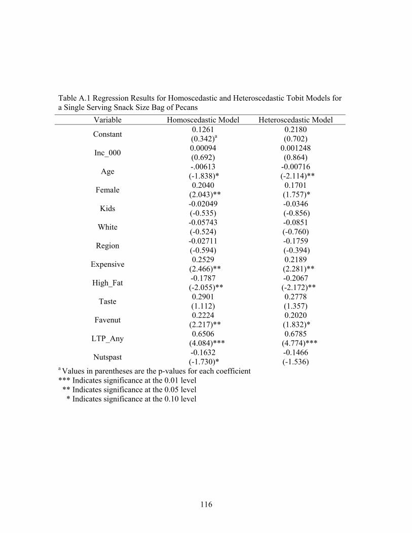
116
Table A.1 Regression Results for Homoscedastic and Heteroscedastic Tobit Models for a Single Serving Snack Size Bag of Pecans
Variable Homoscedastic Model Heteroscedastic Model
Constant 0.1261 (0.342)a
0.2180 (0.702)
Inc_000 0.00094 (0.692)
0.001248 (0.864)
Age -.00613 (-1.838)*
-0.00716 (-2.114)**
Female 0.2040 (2.043)**
0.1701 (1.757)*
Kids -0.02049 (-0.535)
-0.0346 (-0.856)
White -0.05743 (-0.524)
-0.0851 (-0.760)
Region -0.02711 (-0.594)
-0.1759 (-0.394)
Expensive 0.2529 (2.466)**
0.2189 (2.281)**
High_Fat -0.1787 (-2.055)**
-0.2067 (-2.172)**
Taste 0.2901 (1.112)
0.2778 (1.357)
Favenut 0.2224 (2.217)**
0.2020 (1.832)*
LTP_Any 0.6506 (4.084)***
0.6785 (4.774)***
Nutspast -0.1632 (-1.730)*
-0.1466 (-1.536)
a Values in parentheses are the p-values for each coefficient *** Indicates significance at the 0.01 level ** Indicates significance at the 0.05 level * Indicates significance at the 0.10 level