Embed Size (px)
Citation preview

Pumped well
Analytical Versus Numerical Estimates of Water-Level Declines Caused by Pumping,and a Case Study of the Iao Aquifer, Maui, Hawaii
U.S. Department of the InteriorU.S. Geological Survey
Water-Resources Investigations Report 00-4244
Water table with no ppuumping Water table with no pumping
Water table from analytical model with pumping
Water table from 2-D numerical model with pumping
Water table from analytical model with pumping
Water table from 2-D numerical model with pumping

Analytical Versus Numerical Estimates of Water-Level Declines Caused by Pumping, and a CaseStudy of the Iao Aquifer, Maui, Hawaii
By Delwyn S. Oki and William Meyer
U.S. GEOLOGICAL SURVEY
Water-Resources Investigations Report 00-4244
Honolulu, Hawaii2001

U.S. DEPARTMENT OF THE INTERIOR
BRUCE BABBITT, Secretary
U.S. GEOLOGICAL SURVEY
Charles G. Groat, Director
The use of firm, trade, and brand names in this report is for identification purposesonly and does not constitute endorsement by the U.S. Geological Survey.
For additional information write to: Copies of this report can be purchasedfrom:
District Chief U.S. Geological SurveyU.S. Geological Survey Branch of Information Services677 Ala Moana Blvd., Suite 415 Box 25286Honolulu, HI 96813 Denver, CO 80225-0286

Contents iii
CONTENTS
Abstract . . . . . . . . . . . . . . . . . . . . . . . . . . . . . . . . . . . . . . . . . . . . . . . . . . . . . . . . . . . . . . . . . . . . . . . . . . . . . . . . . . . . . . . . . . 1
Introduction . . . . . . . . . . . . . . . . . . . . . . . . . . . . . . . . . . . . . . . . . . . . . . . . . . . . . . . . . . . . . . . . . . . . . . . . . . . . . . . . . . . . . . . 2
Geohydrologic Setting of the Hawaiian Islands . . . . . . . . . . . . . . . . . . . . . . . . . . . . . . . . . . . . . . . . . . . . . . . . . . . . . . . . . . . 3
Hydrologic Effects of Withdrawal From a Ground-Water System . . . . . . . . . . . . . . . . . . . . . . . . . . . . . . . . . . . . . . . . . . . . . 3
Calculation of Sustainable Yield Using the Robust Analytical Model (RAM) . . . . . . . . . . . . . . . . . . . . . . . . . . . . . . . . . . . 6
Comparisons Between RAM and One-Dimensional Numerical Models . . . . . . . . . . . . . . . . . . . . . . . . . . . . . . . . . . . . . . . . 7
Zero Ground-Water Withdrawals . . . . . . . . . . . . . . . . . . . . . . . . . . . . . . . . . . . . . . . . . . . . . . . . . . . . . . . . . . . . . . . . . 8
Ground-Water Withdrawals . . . . . . . . . . . . . . . . . . . . . . . . . . . . . . . . . . . . . . . . . . . . . . . . . . . . . . . . . . . . . . . . . . . . . 10
Comparisons Between RAM and Two-Dimensional Numerical Models . . . . . . . . . . . . . . . . . . . . . . . . . . . . . . . . . . . . . . . . 14
Zero Ground-Water Withdrawals . . . . . . . . . . . . . . . . . . . . . . . . . . . . . . . . . . . . . . . . . . . . . . . . . . . . . . . . . . . . . . . . . 15
Ground-Water Withdrawals . . . . . . . . . . . . . . . . . . . . . . . . . . . . . . . . . . . . . . . . . . . . . . . . . . . . . . . . . . . . . . . . . . . . . 15
Case Study of the Iao Aquifer, Maui. . . . . . . . . . . . . . . . . . . . . . . . . . . . . . . . . . . . . . . . . . . . . . . . . . . . . . . . . . . . . . . . . . . . 19
Geohydrologic Setting . . . . . . . . . . . . . . . . . . . . . . . . . . . . . . . . . . . . . . . . . . . . . . . . . . . . . . . . . . . . . . . . . . . . . . . . . 19
Ground-Water Withdrawals . . . . . . . . . . . . . . . . . . . . . . . . . . . . . . . . . . . . . . . . . . . . . . . . . . . . . . . . . . . . . . . . . . . . . 19
Measured Water Levels and Comparisons with RAM-Predicted Equilibrium Heads . . . . . . . . . . . . . . . . . . . . . . . . . 19
Summary . . . . . . . . . . . . . . . . . . . . . . . . . . . . . . . . . . . . . . . . . . . . . . . . . . . . . . . . . . . . . . . . . . . . . . . . . . . . . . . . . . . . . . . . . 28
References Cited . . . . . . . . . . . . . . . . . . . . . . . . . . . . . . . . . . . . . . . . . . . . . . . . . . . . . . . . . . . . . . . . . . . . . . . . . . . . . . . . . . . 29
Appendix: Description of RAM . . . . . . . . . . . . . . . . . . . . . . . . . . . . . . . . . . . . . . . . . . . . . . . . . . . . . . . . . . . . . . . . . . . . . . . 30
Dupuit Assumption . . . . . . . . . . . . . . . . . . . . . . . . . . . . . . . . . . . . . . . . . . . . . . . . . . . . . . . . . . . . . . . . . . . . . . . . . . . 30
Ghyben-Herzberg Relation. . . . . . . . . . . . . . . . . . . . . . . . . . . . . . . . . . . . . . . . . . . . . . . . . . . . . . . . . . . . . . . . . . . . . . 30
One-Dimensional Analytical Equation . . . . . . . . . . . . . . . . . . . . . . . . . . . . . . . . . . . . . . . . . . . . . . . . . . . . . . . . . . . . 31
FIGURES
1. Schematic cross section of the regional ground-water flow system of the Iao aquifer, Maui, Hawaii . . . . . . . 4
2–7. Diagrams showing:
2. Vertical cross section of the one- and two-dimensional numerical-model grids . . . . . . . . . . . . . . . . . . . . 9
3. Model-calculated steady-state water levels from an analytical model (RAM) and from one-dimensionalnumerical models for conditions of zero withdrawal and withdrawal of 50 percent of the total rechargeto the aquifer for selected caprock confining unit vertical hydraulic-conductivity values:(A) 15 feet per day; (B) 0.15 feet per day; (C) 0.075 feet per day. . . . . . . . . . . . . . . . . . . . . . . . . . . . . . 11
4. Model-calculated steady-state water levels from an analytical model (RAM) and from one-dimensionalnumerical models for conditions of zero withdrawal and withdrawal of 75 percent of the total rechargeto the aquifer for selected caprock confining unit vertical hydraulic-conductivity values:(A) 15 feet per day; (B) 0.15 feet per day; (C) 0.075 feet per day . . . . . . . . . . . . . . . . . . . . . . . . . . . . . 12
5. Model-calculated ratios (from a two-dimensional numerical ground-water flow model) of steady-statewater levels for withdrawal conditions (he) to steady-state predevelopment water levels (h0) in theunconfined part of the aquifer for the case of withdrawing, from a well near the inland extent of theaquifer, 50 percent of the total ground-water recharge . . . . . . . . . . . . . . . . . . . . . . . . . . . . . . . . . . . . . . 16
6. Model-calculated ratios (from a two-dimensional numerical ground-water flow model) of steady-statewater levels for withdrawal conditions (he) to steady-state predevelopment water levels (h0) in theunconfined part of the aquifer for the case of withdrawing, from a well near the middle of theunconfined part of the aquifer, 50 percent of the total ground-water recharge . . . . . . . . . . . . . . . . . . . . 17

iv Analytical Versus Numerical Estimates of Water-Level Declines, and a Case Study of the Iao Aquifer, Maui, Hawaii
7. Model-calculated ratios (from a two-dimensional numerical ground-water flow model) of steady-statewater levels for withdrawal conditions (he) to steady-state predevelopment water levels (h0) in theunconfined part of the aquifer for the case of withdrawing, from a well near the seaward extentof the unconfined part of the aquifer, 50 percent of the total ground-water recharge . . . . . . . . . . . . . . . 18
8–9. Maps showing:
8. Selected wells in the Iao aquifer, Maui, Hawaii . . . . . . . . . . . . . . . . . . . . . . . . . . . . . . . . . . . . . . . . . . . . . 20
9. Surficial geology of the Iao aquifer area, Maui, Hawaii . . . . . . . . . . . . . . . . . . . . . . . . . . . . . . . . . . . . . . . 21
10–12. Graphs of:
10. Water levels at shaft 33 during 1996–98, Iao aquifer, Maui, Hawaii . . . . . . . . . . . . . . . . . . . . . . . . . . . . . 24
11. Water levels at Mokuhau well field, Iao aquifer, Maui, Hawaii . . . . . . . . . . . . . . . . . . . . . . . . . . . . . . . . . 24
12. Water levels at Waiehu deep monitor well and test holes B and E, departure of backward-looking12-month moving average rainfall from the long-term average rainfall for Waiehu Camp rain gage,and monthly mean total withdrawal from the Iao aquifer prior to 1999, Maui, Hawaii . . . . . . . . . . . . . 25
13. Map showing water-level declines in the flank flows of Wailuku Basalt between April 1977 and April1997 for the northern part of the Iao aquifer, Maui, Hawaii . . . . . . . . . . . . . . . . . . . . . . . . . . . . . . . . . . . . . 26
TABLES
1. Ratios of sustainable yield to recharge used by the State of Hawaii Commission on Water ResourceManagement for aquifers in Hawaii . . . . . . . . . . . . . . . . . . . . . . . . . . . . . . . . . . . . . . . . . . . . . . . . . . . . . . . . . . 7
2. Values of leakance for coastal discharge areas in Hawaii . . . . . . . . . . . . . . . . . . . . . . . . . . . . . . . . . . . . . . . . . . . . 103. Differences between model-calculated water levels from RAM and the numerical models at selected sites . . . . . 144. State numbers and names of selected wells in the Iao aquifer, Maui, Hawaii . . . . . . . . . . . . . . . . . . . . . . . . . . . . 225. Annual ground-water withdrawal from the Iao aquifer, Maui, Hawaii . . . . . . . . . . . . . . . . . . . . . . . . . . . . . . . . . . 236. Measured water levels and RAM-predicted equilibrium head (he) at selected wells, Iao aquifer, Maui, Hawaii . 28
Conversion Factors
Multiply By To obtain
foot (ft) 0.3048 meterfoot per day (ft/d) 0.3048 meter per day
million gallons per day (Mgal/d) 0.04381 cubic meter per second

Abstract 1
Abstract
Comparisons were made between model-calculated water levels from a one-dimensionalanalytical model referred to as RAM (Robust Ana-lytical Model) and those from numerical ground-water flow models using a sharp-interface modelcode. RAM incorporates the horizontal-flowassumption and the Ghyben-Herzberg relation torepresent flow in a one-dimensional unconfinedaquifer that contains a body of freshwater floatingon denser saltwater. RAM does not account for thepresence of a low-permeability coastal confiningunit (caprock), which impedes the discharge offresh ground water from the aquifer to the ocean,nor for the spatial distribution of ground-waterwithdrawals from wells, which is significantbecause water-level declines are greatest in thevicinity of withdrawal wells. Numerical ground-water flow models can readily account for dis-charge through a coastal confining unit and for thespatial distribution of ground-water withdrawalsfrom wells.
For a given aquifer hydraulic-conductivityvalue, recharge rate, and withdrawal rate, model-calculated steady-state water-level declines fromRAM can be significantly less than those fromnumerical ground-water flow models. The differ-ences between model-calculated water-leveldeclines from RAM and those from numericalmodels are partly dependent on the hydraulic prop-erties of the aquifer system and the spatial distribu-tion of ground-water withdrawals from wells.RAM invariably predicts the greatest water-level
declines at the inland extent of the aquifer wherethe freshwater body is thickest and the potential forsaltwater intrusion is lowest. For cases in which alow-permeability confining unit overlies the aqui-fer near the coast, however, water-level declinescalculated from numerical models may exceedthose from RAM even at the inland extent of theaquifer.
Since 1990, RAM has been used by the Stateof Hawaii Commission on Water Resource Man-agement for establishing sustainable-yield valuesfor the State’s aquifers. Data from the Iao aquifer,which lies on the northeastern flank of the WestMaui Volcano and which is confined near the coastby caprock, are now available to evaluate the pre-dictive capability of RAM for this system. In 1995and 1996, withdrawal from the Iao aquifer reachedthe 20 million gallon per day sustainable-yieldvalue derived using RAM. However, even before1996, water levels in the aquifer had declined sig-nificantly below those predicted by RAM, and con-tinued to decline in 1997. To halt the decline ofwater levels and to preclude the intrusion of salt-water into the four major well fields in the aquifer,it was necessary to reduce withdrawal from theaquifer system below the sustainable-yield valuederived using RAM.
In the Iao aquifer, the decline of measuredwater levels below those predicted by RAM is con-sistent with the results of the numerical model ana-lysis. Relative to model-calculated water-leveldeclines from numerical ground-water flow mod-els, (1) RAM underestimates water-level declines
Analytical Versus Numerical Estimates of Water-LevelDeclines Caused by Pumping, and a Case Study of theIao Aquifer, Maui, Hawaii
By Delwyn S. Oki and William Meyer

2 Analytical Versus Numerical Estimates of Water-Level Declines, and a Case Study of the Iao Aquifer, Maui, Hawaii
in areas where a low-permeability confining unitexists, and (2) RAM underestimates water-leveldeclines in the vicinity of withdrawal wells.
INTRODUCTION
A one-dimensional analytical model of ground-water flow, known as the Robust Analytical Model(RAM) (Mink, 1980), is a commonly used tool for esti-mating sustainable-yield values for aquifer systems inHawaii. Sustainable yield, as defined by the State ofHawaii, refers to “the maximum rate at which watermay be withdrawn from a water source without impair-ing the utility or quality of the water source...” (State ofHawaii, 1987). The definition “unequivocally incorpo-rates infinite time as a fundamental condition” of thesustainable-yield estimate (State of Hawaii, 1992,p. 98). In Hawaii, the most common limitation on therate of withdrawal from an aquifer is the upward move-ment (into wells) of the brackish-water transition zonebetween freshwater and saltwater. To preclude salt-water intrusion at a given location, it is necessary tomaintain a sufficient water level at that location. Esti-mates of sustainable yield, therefore, require accurateestimates of the water levels in a ground-water systemfor a given distribution and rate of ground-water with-drawal.
To estimate the amount of water available from aground-water system on a long-term basis, water-leveldeclines and the changes in the magnitude and distribu-tion of recharge or discharge within the system causedby withdrawals need to be estimated. These factors are,in turn, dependent on: (1) the hydraulic properties of thesystem, (2) boundary conditions (hydrogeologic fea-tures at the physical limits of the system), and (3) thepositioning of development (wells) within the system(Bredehoeft and others, 1982).
RAM does not account for aquifer boundary con-ditions that commonly exist in Hawaii, nor for the spa-tial distribution of ground-water withdrawals fromwells (RAM is one dimensional). Implicit in the use ofRAM are the assumptions that (1) sustainable yield canbe estimated without accounting for aquifer boundaryconditions, aquifer geometry, and the spatial distribu-tion of hydraulic properties of the system, and (2) sus-tainable yield is an intrinsic property of an aquifer
independent of the locations of wells and rates of with-drawal from wells.
One of the more important boundary conditionsthat RAM cannot represent is a low-permeability con-fining unit that exists over the volcanic-rock aquifersnear and beyond the shoreline in many areas of the State(see, for example, Hunt, 1996; Meyer and Presley,2000). Among the volcanic-rock aquifers that are over-lain by a low-permeability confining unit are the twomost important aquifers in the State, the Pearl Harboraquifer on Oahu and the Iao aquifer on Maui. [For thepurposes of this report, the Iao aquifer system, as delin-eated by State Commission on Water Resource Man-agement (CWRM), is referred to as the Iao aquiferalthough it is recognized that the Iao aquifer system ispart of a regional ground-water flow system.] The con-fining unit is formed by a wedge-shaped layer of terres-trial or marine sediments of relatively low permeabilityand is referred to as caprock in Hawaii. A caprockimpedes the discharge of freshwater from the aquifer tothe ocean and is an important control on the ultimatewater-level decline caused by ground-water withdraw-als from the aquifer.
In 1995 and 1996, withdrawal from the Iao aquiferreached the sustainable-yield value derived usingRAM. However, even before 1996, water levels in theaquifer had declined significantly below those predictedby RAM, and were still declining in 1997. As a result,withdrawal from the aquifer was reduced below thesustainable-yield value derived using RAM to halt thedecline of water levels and preclude the intrusion ofsaltwater into the four major well fields in the aquifer.
Purpose and scope.--The purpose of this report isto describe (1) comparisons between model-calculatedwater levels from RAM and those from numericalground-water flow models that account for appropriateaquifer boundary conditions and spatially distributedwithdrawals, and (2) a case study of the Iao aquifer,Maui, where water levels have declined below altitudespredicted by RAM. A site-specific numerical ground-water flow model of the Iao aquifer was not developedfor this study. Rather, generic one- and two-dimen-sional numerical ground-water flow models were usedto simulate water-level declines for highly permeableaquifers overlain by caprock near the coast. All numer-ical models used a sharp-interface code (Essaid, 1990)that simulates flow in ground-water systems containingfreshwater and saltwater.

Geohydrologic Setting of the Hawaiian Islands 3
GEOHYDROLOGIC SETTING OF THEHAWAIIAN ISLANDS
The main islands of Hawaii consist of one or morevolcanoes that were formed by submarine and subaerialeruptions. During the principal stage of volcano build-ing, called the shield stage, thousands of lava flowsemanate from a central caldera and from two to three riftzones that extend outward from the caldera. Magmamay cool and solidify beneath the surface of the volcanoand form thin, dense, massive, nearly vertical sheets ofintrusive rock known as dikes. Within and near thecaldera and rift zones, lava flows are intruded bynumerous dikes. Outside the zone containing dikes, lavaflows extend to the ocean without intrusions. These lat-ter flows are commonly referred to as flank flows inHawaii. In many coastal areas of the State, lava flowsare overlain by sedimentary deposits that form a confin-ing unit, called caprock, above the volcanic-rock aqui-fer.
In qualitative terms, permeability describes theease with which fluid can move through a porous rock(see, for example, Domenico and Schwartz, 1990). Per-meability of dike-free volcanic rocks in Hawaii ishighly variable, depending to some degree on the thick-ness of individual lava flows and the extent of weather-ing that individual flows have undergone. Hydraulicconductivity is a quantitative measure of the capacity ofa rock to transmit water. The horizontal hydraulic con-ductivity of the dike-free volcanic rocks of central Oahuand western Hawaii generally is high (on the order of1,000 ft/d or more) (Hunt, 1996; Oki, 1999), whereasthe horizontal hydraulic conductivity of the volcanicrocks of eastern Kauai and northeastern Maui generallyis low (on the order of 1 ft/d or less) (Izuka and Ginger-ich, 1998; Gingerich, 1998; Gingerich, 1999). The lowhydraulic conductivity of volcanic rocks of easternKauai and northeastern Maui may partly be caused bythe presence of dikes.
Ground-water recharge rates in Hawaii varygreatly and are dependent on factors such as soil prop-erties, land cover, and rates of rainfall, evaporation, andrunoff. In southern Oahu, recharge has been estimatedto range from about 16 to 21 Mgal/d per mile of aquiferwidth (measured parallel to the coast), depending onland-use conditions (Giambelluca, 1986). In drier areas,such as the western part of the island of Hawaii (Oki andothers, 1999), recharge may be as low as 3 Mgal/d permile of aquifer width.
Fresh ground water in the Hawaiian islands isfound mainly as: (1) a freshwater-lens system (withwater levels commonly less than a few tens of feetabove sea level) consisting of a lens-shaped body offreshwater floating on and displacing saltwater withindike-free volcanic rocks, (2) dike-impounded water(with water levels that are tens to thousands of feetabove sea level) where overall permeability is low dueto the presence of dikes, and (3) as perched water. Theprincipal source of fresh ground water for domestic usein the Hawaiian islands is from freshwater-lens systemswithin the highly permeable dike-free parts of volcanic-rock aquifers, such as the Pearl Harbor aquifer on Oahuand the Iao aquifer on Maui.
Where the permeability of dike-free volcanic rocksis relatively high (hydraulic-conductivity values greaterthan about 1,000 ft/d), predevelopment water levels inthe freshwater-lens system generally are less than 50 ftabove sea level. Where the permeability of the dike-freevolcanic rocks is relatively low (hydraulic-conductivityvalues less than about 1 ft/d), predevelopment waterlevels can range from several hundred to several thou-sands of feet above sea level, forming a vertically exten-sive freshwater-lens system.
The general movement of fresh ground water isfrom mountainous interior areas to coastal dischargeareas (fig. 1). Ground water discharges into the ocean orstreams or by evapotranspiration near the shoreline.Near coastal discharge areas, movement of fresh groundwater in a freshwater-lens system is predominantlyupward and across the layered sequence of lava flowsand the caprock, where it exists.
HYDROLOGIC EFFECTS OFWITHDRAWAL FROM A GROUND-WATERSYSTEM
The effects of withdrawal on water levels and dis-charge can be understood most readily by considering asimple, finite ground-water flow system in which theonly source of recharge is from precipitation and all dis-charge is to the ocean. If the rate of recharge to thisground-water system remains unchanged over time, andif there are no ground-water withdrawals, a predevelop-ment equilibrium or steady-state condition will eventu-ally be reached in which ground-water levels do notvary with time and the rate of discharge from the systemis equal to the rate of recharge.

4 Analytical Versus Numerical Estimates of Water-Level Declines, and a Case Study of the Iao Aquifer, Maui, Hawaii
02,
000
4x V
ER
TIC
AL
EX
AG
GE
RA
TIO
N
4,00
0 F
EE
T
4,00
0
FE
ET
3,50
0
3,00
0
2,50
0
2,00
0
1,50
0
1,00
0
500
SE
ALE
VE
L
-500
-1,0
00
-1,5
00
VO
LCA
NIC
RO
CK
S
SE
DIM
EN
TA
RY
DE
PO
SIT
S
GE
NE
RA
LIZ
ED
DIR
EC
TIO
N O
F G
RO
UN
D-W
AT
ER
F
LOW
WA
TE
R T
AB
LE
DIK
ES
Oce
an
saltw
ater
saltw
ater
fres
hwat
erfr
eshw
ater
tran
sitio
n zo
ne
tran
sitio
n zo
ne
EX
PLA
NAT
ION
Dik
e-im
poun
ded
grou
nd w
ater
Boundary between dike-impounded
ground water and freshwater-lens system
Fig
ure
1. S
chem
atic
cro
ss s
ectio
n of
the
regi
onal
gro
und-
wat
er fl
ow s
yste
m o
f the
Iao
aqui
fer,
Mau
i, H
awai
i.

Hydrologic Effects of Withdrawal From a Ground-Water System 5
When withdrawal from a well begins, water is ini-tially removed from aquifer storage in the vicinity of thewell, and water levels in the vicinity of the well begin todecline. If withdrawal from the well continues at a con-stant rate, the zone over which water levels declineexpands outward from the well as additional water isremoved from storage. Water-level decline is greatest atthe withdrawal site and decreases outward from the wellforming what is known as a cone of depression. Thecone of depression eventually reaches an area wherewater is discharging to the ocean. As water levelsdecline near the discharge area, the rate of discharge tothe ocean decreases. If and when the reduction of dis-charge rate to the ocean is equal to the rate of with-drawal, a new steady-state condition is reached andwater levels cease to decline further. The magnitude ofthe ultimate water-level decline caused by withdrawal isaffected by factors including (1) the rate of withdrawal,(2) the hydraulic properties of the aquifer system, and(3) the location of the withdrawal site relative to the dis-charge boundary of the system. These factors are brieflydescribed in the following paragraphs.
Rate of withdrawal.--All other factors being equal,higher rates of withdrawal cause greater water-leveldeclines than lower rates of withdrawal. This is intu-itively clear considering that for a withdrawal rate ofzero water levels will not decline, and that for a smallbut positive withdrawal rate water levels will decline tosome extent.
Hydraulic properties of the aquifer system.--Thehydraulic properties at the discharge boundary of thesystem have an effect on the magnitude of the ultimatewater-level decline caused by withdrawal. The lowerthe permeability of the coastal confining unit, thegreater is the water-level decline at the dischargeboundary necessary to reduce an equal amount of dis-charge from the system. This is explained by first con-sidering the case of injecting rather than withdrawingwater from a system. Assuming that water is injected ata steady rate for a period sufficiently long to reachsteady-state conditions, water levels at the dischargeboundary increase to a greater extent (relative to thepre-injection, steady-state condition) the lower the per-meability of the confining unit at the discharge bound-ary because greater hydraulic head is required to forcean equal amount of discharge through a low-permeabil-ity confining unit than a high-permeability unit.(Hydraulic head at a given point is commonly measuredby water levels in wells that are open to the aquifer only
at that point.) Thus, to return back to the original, pre-injection, steady-state condition following the cessationof injection, the lower the permeability of the confiningunit the greater is the water-level decline at the dis-charge boundary necessary to reduce an equal amountof discharge from the system.
Location of the withdrawal site.--The location ofthe withdrawal site relative to the discharge boundaryhas an effect on the magnitude of the water-leveldecline at the withdrawal site. Consider the case of aone-dimensional, finite aquifer system that is in asteady-state condition prior to any withdrawal. Steadywithdrawal from a well at the inland extent of the dis-charge boundary will cause water levels to decline to anew steady-state level at which the reduction of dis-charge rate is equal to the withdrawal rate. Because thecone of depression caused by withdrawal from a well isdeepest at the well, water-level declines decrease inlandfrom the well. Consider next the case of a well with-drawing at the same rate as in the previous case butlocated at the inland extent of an identical one-dimen-sional aquifer system. All other factors being equal,withdrawal from a well at the inland extent of the aqui-fer will cause water levels to decline at the dischargeboundary, and at the inland extent of the dischargeboundary, to the same level as in the previous casebecause steady-state discharge to the ocean is the samein both cases. As in the previous case, water-leveldeclines are greatest at the withdrawal site and, there-fore, water-level declines increase from the inlandextent of the discharge boundary toward the well. Thus,the water-level decline at an inland withdrawal site isgreater than the water-level decline at a withdrawal sitenear the discharge boundary, all other factors beingequal.
In most situations, the source of water derivedfrom wells is from decreased ground-water storage anddecreased ground-water discharge. In the above discus-sion, ground-water discharge was limited to the ocean,which is sometimes the case in Hawaii. However, insome ground-water systems (including those inHawaii), discharge may be to streams and surface-waterbodies other than the ocean, or by evapotranspirationfrom plants that have roots extending to ground water.Thus, withdrawal from a well may cause a reduction ofdischarge to streams and other surface-water bodies, ordecreased evapotranspiration by plants if the water tableis lowered below the level of the roots. In addition, thesource of water derived from wells may be from

6 Analytical Versus Numerical Estimates of Water-Level Declines, and a Case Study of the Iao Aquifer, Maui, Hawaii
increased recharge. For example, reduction of ground-water levels by withdrawal may induce flow from astream into the ground-water system or may increaserecharge by capturing water that was originally runoffwhen water levels were at or near the surface.
The hydrologic analysis of a ground-water systemgenerally requires construction of a numerical ground-water flow model. If appropriately constructed, anumerical model can represent the complex relationsamong the inflows, outflows, changes in storage, move-ment of water in the system, and other important fea-tures.
CALCULATION OF SUSTAINABLE YIELDUSING THE ROBUST ANALYTICALMODEL (RAM)
The one-dimensional RAM used by CWRM toestimate sustainable yield in Hawaii incorporates thehorizontal-flow assumption (see, for example, Bear,1972) and the Ghyben-Herzberg relation and isdescribed in detail in the appendix. By the assumptionsused to derive RAM (Mink, 1980), for any location inthe aquifer, the ratio of the hydraulic head squared to thetotal flow rate through the aquifer is constant. Thus, thefollowing relation is assumed to be true:
h02/Q0 = he
2/Qe, (1)
where, h0 = hydraulic head [L], relative to mean sealevel, at locationx for flow rateQ0,
Q0 = steady-state rate of flow through aquiferfor predevelopment conditions[L3/T],
he = hydraulic head [L], relative to mean sealevel, at locationx for flow rateQe,
Qe = steady-state rate of flow (lesswithdrawals from wells or shafts)through aquifer for developmentconditions [L3/T], and
x = Cartesian coordinate [L].
Calculation of sustainable yield using RAMinvolves pre-selection of the steady-state water levelthat will occur if ground water is withdrawn at a rateequal to the sustainable yield. This water level isreferred to as the equilibrium head (he). For the desiredequilibrium head,he, CWRM defines the sustainableyield,D, as the difference between the predevelopment
rate of flow through the aquifer minus the reduced rateof flow through the aquifer following development:
D = Q0 − Qe. (2)
Combining equations (1) and (2), and definingI tobe equal toQ0 yields:
D/I = 1− (he/h0)2. (3)
Equation (3) represents the model (RAM) com-monly used to set sustainable yield in Hawaii. To applythis equation, predevelopment values forh0 andI mustbe known or estimated, and some desired minimumequilibrium head,he, must be established. In manyareas, values forh0 are poorly known and must there-fore be estimated. The value forI is generally equatedto the recharge from a water budget of predevelopmentconditions. The value forhe is selected to preserve thequality of water produced at steady-state conditions(State of Hawaii, 1992, p. B3).
In Hawaii, RAM is used for all freshwater-lenssystems and in areas where dike-impounded water isdominant or extends to the coast (State of Hawaii, 1992,p. 120). According to the State Water Resources Protec-tion Plan, where the initial head,h0, in the aquifer waslow, the ratiohe:h0 must be large and the ratioD:I mustbe small (State of Hawaii, 1992, p. B3). Also accordingto the State Water Resources Protection Plan, the ratiohe:h0 “used to obtain sustainable yield is based on expe-rience with known aquifers, such as those of Honoluluand southern Oahu” (State of Hawaii, 1992, p. B4). Val-ues ofhe:h0 andD:I used by CWRM for given values ofh0 are shown in table 1.
Limitations of RAM.--One of the major limita-tions of RAM for use in estimating sustainable yield inHawaii is the inability of the model to account for thecaprock, which creates resistance to vertical dischargeof ground water from the aquifer to the ocean. The over-all vertical hydraulic conductivity of dike-free volcanicrocks (including weathered zones) and the caprock isgenerally one to four orders of magnitude less than thehorizontal hydraulic conductivity of the dike-free vol-canic rocks. Thus, the resistance to vertical discharge ofground water to the ocean is much greater per unit areathan the resistance to horizontal ground-water flow inthe aquifer. The rate of vertical discharge is propor-tional to the overall vertical hydraulic conductivity ofthe volcanic rocks and caprock divided by the thickness

Comparisons Between RAM and One-Dimensional Numerical Models 7
of these two rock units. The ratio of vertical hydraulicconductivity to thickness is known as leakance:
L = Kv /B (4)
where, L = leakance [1/T],Kv = overall vertical hydraulic conductivity of
the rocks where vertical dischargeoccurs [L/T], and
B= overall rock thickness over whichvertical discharge occurs [L].
RAM does not account for the concept of leakancealthough leakance is “all important” in controlling theresponse of ground-water systems to stresses (Brede-hoeft and Hall, 1995). Leakance is important becausefor withdrawal to be sustained in most areas of Hawaii,natural discharge into the ocean must be reduced by anamount equal or nearly equal to withdrawal. Thesmaller the value of leakance (or the greater the resis-tance to the diversion of water to wells), the greater isthe water-level decline necessary to reduce an equalamount of natural discharge, and the greater the water-level decline in the well or wells. Because RAM doesnot account for the presence of a caprock and the con-cept of leakance, RAM cannot accurately predict water-level declines associated with withdrawals in manyHawaiian ground-water systems due to this limitationalone.
In addition to its inability to represent a caprock,RAM cannot account for spatially distributed with-drawals from wells and the spatial distribution of water-level declines, which are greatest in the vicinity of with-drawal wells. As will be shown in the following sec-tions, the one-dimensional RAM invariably predicts thegreatest water-level declines at the inland extent of theaquifer where the freshwater lens is thickest and thepotential for saltwater intrusion is lowest.
Because RAM is a one-dimensional model, it can-not accurately account for the spatial distribution ofrecharge. RAM assumes that all recharge enters theground-water flow system at the inland extent of thesystem. Furthermore, because RAM is a one-dimen-sional model, it cannot adequately account for thegeometry of the ground-water flow system. RAM alsocannot account for the spatial variability of aquiferhydraulic properties, which affects the distribution ofwater-level declines caused by withdrawals.
In the following sections of this report, model-calculated water-level declines from RAM are com-pared with model-calculated water-level declines fromone- and two-dimensional numerical ground-waterflow models. One-dimensional numerical models areused to demonstrate the importance of the caprock onthe hydrologic response of the ground-water system towithdrawals, and two-dimensional (areal) numericalmodels are used to demonstrate the importance of rep-resenting the spatial distribution of ground-water with-drawals from wells. (By addressing the spatialdistribution of withdrawals, the two-dimensional mod-els also indirectly address the importance of properlyrepresenting the spatial distribution of recharge.)
COMPARISONS BETWEEN RAM ANDONE-DIMENSIONAL NUMERICALMODELS
A simple one-dimensional ground-water flow sys-tem was used to compare model-calculated water levelsfrom RAM with steady-state water levels from sharp-interface numerical ground-water flow models. Thenumerical code used was SHARP (Essaid, 1990), whichsimulates flow in ground-water systems containingfreshwater and saltwater and treats freshwater and salt-water as immiscible fluids separated by a sharp inter-
Table 1. Ratios of sustainable yield to recharge used by the State of Hawaii Commission on Water ResourceManagement for aquifers in Hawaii (State of Hawaii, 1990)
Initial head, h0,in feet above sea level
Ratio of equilibrium head toinitial head, he:h0
Ratio of sustainable yield torecharge, D:I
4–10 0.75 0.4411–15 0.70 0.5116–20 0.65 0.5821–25 0.60 0.64
>26 0.50 0.75

8 Analytical Versus Numerical Estimates of Water-Level Declines, and a Case Study of the Iao Aquifer, Maui, Hawaii
face. The ground-water flow system was assumed toconsist of an aquifer that is unconfined inland and thatis confined by a caprock near the shore and offshore.The numerical model grid used to represent the flowsystem consists of 44 cells; each cell is 2,000 ft long andextends to a depth of 6,000 ft below sea level (fig. 2).
Recharge to the system was assumed to be a con-stant value of 20 Mgal/d per mile of aquifer width andenter the system at the inland extent of the aquifer. Therestriction that recharge enter the system at the inlandextent of the aquifer is necessary because RAM cannotrepresent spatially varying recharge.
The horizontal hydraulic conductivity of the aqui-fer was assumed to be a constant value of 1,500 ft/d,corresponding to a highly permeable volcanic-rockaquifer. The analysis was restricted to highly permeablevolcanic-rock aquifers because vertical head gradientsare expected to be small in magnitude relative to verti-cal head gradients in poorly permeable aquifers. BothRAM and the numerical models used in this studyassume that flow is horizontal, a condition which is lesslikely to occur in poorly permeable aquifers.
The confining unit that overlies the aquifer near thecoast is represented in the numerical models as a sea-ward-thickening wedge of coastal sedimentary depositsthat is 40 ft thick at the inland extent of the confiningunit and 1,000 ft thick at the shore (fig. 2). Offshore, thecaprock is assumed to have a constant thickness of1,000 ft. Discharge through the caprock is assumed tobe in the vertical direction. Three different values ofcaprock vertical hydraulic conductivity were testedwith numerical models: 15, 0.15, and 0.075 ft/d. Thevertical hydraulic-conductivity value of 0.15 ft/d is rep-resentative of the Pearl Harbor aquifer of southern Oahu(Souza and Voss, 1987). The range of leakance valuesrepresented in the one-dimensional numerical models isabout 0.000075 (=0.075/1,000) to 0.375 (=15/40) feetper day per foot. The range of leakance values tested isconsistent with the range of values estimated for Hawai-ian ground-water flow systems (table 2).
Discharge from the aquifer to the ocean was mod-eled as a head-dependent discharge boundary condition.The rate of freshwater discharge is assumed to be lin-early related to the leakance and head in the aquiferaccording to the equation:
Q = LAc(h − h′) (5)
where, Q = rate of discharge from the aquifer [L3/T],L = confining unit leakance, [1/T],
Ac = plan area of confining unit [L2],h = hydraulic head in the aquifer [L], relative
to mean sea level, at the dischargeboundary, and
h′ = hydraulic head above the confining unit[L], relative to mean sea level.
For onshore areas,h′ was assumed to be equal tozero. For offshore areas,h′ was assigned a value corre-sponding to the freshwater-equivalent head of the salt-water column overlying the ocean floor within the cell.The freshwater-equivalent head, measured relative to amean sea level datum, was computed from the equation:
h′ = –Z/40, (6)
whereZ is the altitude of the ocean floor.
Zero Ground-Water Withdrawals
For zero ground-water withdrawals, model-calcu-lated steady-state water levels from the numerical mod-els were 6.3, 30.6, and 52.5 ft above sea level at theseaward extent of the unconfined part of the system forcaprock vertical hydraulic-conductivity values of 15,0.15, and 0.075 ft/d, respectively (figs. 3 and 4). Lowervertical hydraulic-conductivity values for the caprockresult in a greater resistance to discharge and higherwater levels.
In the absence of ground-water withdrawals, ananalytical equation (see equation a4 in the appendix)that forms the basis of RAM can be used to compute thesteady-state water-table profile in a one-dimensionalaquifer if the water level is known at the seaward extentof the unconfined part of the aquifer. To allow for directcomparisons between the analytical equation andnumerical models, the water level at the seaward extentof the unconfined part of the aquifer for the analyticalequation was assigned the same value as the corre-sponding water level from the numerical model. Thus,in the analytical equation, the water level at the seawardextent of the unconfined part of the aquifer wasassigned values of 6.3, 30.6, and 52.5 ft above sea levelfor the three different cases, corresponding to the threecaprock vertical hydraulic-conductivity values testedwith the numerical models. For zero ground-water with-drawals, the model-calculated water-table profiles fromthe numerical models are in close agreement with the

Comparisons Between RAM and One-Dimensional Numerical Models 9
1011
1213
1415
1617
181
23
45
67
89
1920
2122
2324
2526
2728
2930
3132
3334
3536
3738
3940
4142
4344
Sea
Lev
el
1,00
0
FE
ET
-1,0
00
-2,0
00
-3,0
00
-4,0
00
-5,0
00
-6,0
00
Coastline
Seaward extent of unconfined aquiferand inland extent
of caprock
Con
finin
g un
it (c
apro
ck)
No-
flow
bou
ndar
y ce
ll
No-
flow
bou
ndar
y ce
ll
010
,000
20,0
00 F
EE
T
Hor
izon
tal S
cale
CE
LL N
UM
BE
R
Fig
ure
2. V
ertic
al c
ross
sec
tion
of th
e on
e- a
nd tw
o-di
men
sion
al n
umer
ical
-mod
el g
rids.
Mod
el c
ells
2 to
15
of th
e on
e-di
men
-si
onal
mod
elgr
id(c
orre
spon
ding
toro
ws
2to
15of
the
two-
dim
ensi
onal
mod
elgr
id)
are
unco
nfine
d,w
ater
-tab
lece
lls.M
odel
cells
16 to
43
of th
e on
e-di
men
sion
al m
odel
grid
(co
rres
pond
ing
to r
ows
16 to
43
of th
e tw
o-di
men
sion
al m
odel
grid
) ar
e he
ad-d
epen
-de
nt d
isch
arge
cel
ls. A
ll m
odel
cel
ls a
re 2
,000
feet
long
. Rec
harg
e is
intr
oduc
ed in
to m
odel
cel
l 2 o
f the
one
-dim
ensi
onal
mod
elgr
id(r
ow2
for
the
two-
dim
ensi
onal
mod
elgr
id).
For
the
one-
dim
ensi
onal
mod
el,p
umpi
ngis
sim
ulat
edfr
omce
lls2,
9,or
15,c
orre
-sp
ondi
ng to
pum
ping
from
nea
r th
e in
land
ext
ent,
mid
dle,
or
seaw
ard
exte
nt, r
espe
ctiv
ely,
of t
he u
ncon
fined
par
t of t
he a
quife
r.

10 Analytical Versus Numerical Estimates of Water-Level Declines, and a Case Study of the Iao Aquifer, Maui, Hawaii
water-table profiles from the analytical equation (figs. 3and 4).
Ground-Water Withdrawals
For ground-water systems in Hawaii with a low-permeability coastal confining unit, predevelopmentwater levels generally ranged from about 10 to 40 ftabove sea level. For these systems, CWRM assumesthat at least 50 percent of the total ground-waterrecharge to the aquifer can be withdrawn (table 1). Forsystems with predevelopment water levels greater than26 ft above sea level, CWRM assumes that as much as75 percent of the total recharge to the aquifer can bewithdrawn (table 1). Thus, the one-dimensional numer-ical models were used to simulate steady-state waterlevels that result from withdrawing 50 percent (fig. 3) or75 percent (fig. 4) of the recharge to the aquifer.
Water-table profiles were simulated for each ofthree caprock vertical hydraulic-conductivity values(0.075, 0.15, and 15 ft/d) and for each of three differentlocations of withdrawal (at the inland extent of theunconfined part of the aquifer, near the middle of theunconfined part of the aquifer, and near the seawardextent of the unconfined part of the aquifer). The sea-ward extent of the unconfined part of the aquifer is thesame as the inland extent of the caprock dischargeboundary. In a one-dimensional model, withdrawal isimplicitly assumed to occur uniformly along the entirewidth of the aquifer. In the numerical model, the simu-lated withdrawal was restricted to the freshwater part ofthe system; that is, no saltwater was withdrawn. Resultsfrom this study are consistent with results from pub-lished numerical models, which have shown that lea-kance is one of the major factors controlling theresponse of ground-water systems to natural or imposed
stresses in Hawaii (Underwood and others, 1995; Oki,1997; Oki, 1998).
The model-calculated water-table profiles from thenumerical models (figs. 3 and 4) indicate that, for agiven withdrawal rate and location, lower values ofcaprock vertical hydraulic conductivity cause greaterwater-level declines relative to predevelopment (zerowithdrawal) conditions. As described previously, thelower the value of caprock vertical hydraulic conductiv-ity (or leakance), the greater is the steady-state water-level decline needed to reduce an equal amount of nat-ural discharge (see the section “Hydrologic Effects ofWithdrawal from a Ground-Water System”).
The model-calculated water-table profiles (figs. 3and 4) from the numerical models also indicate that fora given value of caprock vertical hydraulic conductivityand withdrawal rate (1) the water-level declines at theinland extent of the discharge boundary (caprock) arethe same regardless of where the withdrawal site islocated inland from the caprock, and (2) water-leveldeclines at withdrawal sites are greater for inland with-drawal sites than for withdrawal sites near the caprock.These results are consistent with the expected responseof a ground-water system to withdrawal (see the section“Hydrologic Effects of Withdrawal from a Ground-Water System”).
RAM also was used to compute the water-tableprofiles that would result if either 50 or 75 percent of thetotal 20 Mgal/d per mile recharge was withdrawn (figs.3 and 4). By the assumptions of RAM, all ground-waterwithdrawals are assumed to occur at the inland extent ofthe aquifer because withdrawals are represented as areduction in recharge. RAM predicts that if 50 percentof the recharge is withdrawn, then the resulting steady-state water levels are uniformly 0.707 (equal to thesquare root of 0.5) multiplied by the predevelopment
aLeakance is dependent on the thickness of the confining unit and is therefore spatially variable.
Table 2. Values of leakance for coastal discharge areas in Hawaii
AreaLeakance
(feet per day per foot) Reference
Oahu, northern 0.00007–1a Oki, 1998Oahu, southern 0.00001–0.03a Oki, 1998Oahu, southeastern 0.0004–0.03a Eyre and others, 1986Molokai, northern 0.1 Oki, 1997Molokai, southern 0.001–0.3a Oki, 1997Hawaii, northwestern 0.01–0.1 Underwood and others, 1995Hawaii, western 0.05 Oki, 1999

Comparisons Between RAM and One-Dimensional Numerical Models 11
05,
000
10,0
0015
,000
20,0
0025
,000
30,0
000
5,00
010
,000
15,0
00D
IST
AN
CE
FR
OM
INLA
ND
EX
TE
NT
OF
CA
PR
OC
K, I
N F
EE
T20
,000
25,0
0030
,000
05,
000
10,0
0015
,000
20,0
0025
,000
30,0
00
0102030405060 -10-50510
-400
-300
-200
-1000
100
200
300
400
MODEL-CALCULATEDWATER LEVEL,
IN FEET ABOVE SEA LEVEL
DIFFERENCE INMODEL-CALCULATED WATER LEVELS FROM
AN ANALYTICAL MODEL AND
NUMERICAL MODELS, IN FEET
DIFFERENCE INMODEL-CALCULATED
INTERFACE ALTITUDES FROMAN ANALYTICAL
MODEL ANDNUMERICAL MODELS, IN FEET
Cap
rock
ver
tical
hyd
raul
ic c
ondu
ctiv
ity o
f 15
feet
per
day
Cap
rock
ver
tical
hyd
raul
ic c
ondu
ctiv
ity o
f 0.1
5 fe
et p
er d
ayC
apro
ck v
ertic
al h
ydra
ulic
con
duct
ivity
of 0
.075
feet
per
day
AB
C
EX
PLA
NA
TIO
N
ZE
RO
WIT
HD
RA
WA
L10
MG
AL/
D P
ER
MIL
E W
ITH
DR
AW
AL
(50
PE
RC
EN
T O
F R
EC
HA
RG
E)
AN
ALY
TIC
AL
MO
DE
LN
UM
ER
ICA
L M
OD
EL
AN
ALY
TIC
AL
MO
DE
L, W
ITH
DR
AW
AL
AT
INLA
ND
EX
TE
NT
OF
SY
TS
EM
NU
ME
RIC
AL
MO
DE
L, W
ITH
DR
AW
AL
AT
SE
AW
AR
D E
XT
EN
T O
F U
NC
ON
FIN
ED
AQ
UIF
ER
NU
ME
RIC
AL
MO
DE
L, W
ITH
DR
AW
AL
NE
AR
MID
DLE
OF
UN
CO
NF
INE
D A
QU
IFE
RN
UM
ER
ICA
L M
OD
EL,
WIT
HD
RA
WA
L A
T IN
LAN
D E
XT
EN
T O
F S
YS
TE
M
Shaded where the analytical model (RAM) predicts higherwater levels than the numerical models
Shaded where the analytical model (RAM) predicts deeperinterface altitudes than the numerical models
Fig
ure
3. M
odel
-cal
cula
ted
stea
dy-s
tate
wat
er le
vels
from
an
anal
ytic
al m
odel
(R
AM
) an
d fr
om o
ne-d
imen
sion
al n
umer
ical
mod
els
for
cond
ition
s of
zer
o w
ithdr
awal
and
with
draw
al o
f 50
perc
ent o
f the
tota
l rec
harg
e to
the
aqui
fer
for
sele
cted
cap
rock
con
finin
g un
it ve
rtic
alhy
drau
lic-c
ondu
ctiv
ityva
lues
:(A
)15
feet
perd
ay;(
B)0
.15
feet
perd
ay;(
C)0
.075
feet
perd
ay.A
lso
show
nar
eth
edi
ffere
nces
betw
een
the
mod
el-c
alcu
late
d w
ater
leve
ls (
and
inte
rfac
e al
titud
es)
from
the
anal
ytic
al m
odel
and
one
-dim
ensi
onal
num
eric
al m
odel
s fo
r w
ithdr
awal
cond
ition
s.A
quife
rhy
drau
licco
nduc
tivity
is1,
500
feet
per
day,
and
grou
nd-w
ater
rech
arge
is20
mill
ion
gallo
nspe
rda
ype
rm
ileof
aqui
fer
wid
th. A
ll re
char
ge e
nter
s th
e sy
stem
at t
he in
land
ext
ent o
f the
aqu
ifer.

12 Analytical Versus Numerical Estimates of Water-Level Declines, and a Case Study of the Iao Aquifer, Maui, Hawaii
05,
000
10,0
0015
,000
20,0
0025
,000
30,0
000
5,00
010
,000
15,0
0020
,000
25,0
0030
,000
05,
000
10,0
0015
,000
20,0
0025
,000
30,0
00
0102030405060 -10-50510
-400
-300
-200
-1000
100
200
300
400
Cap
rock
ver
tical
hyd
raul
ic c
ondu
ctiv
ity o
f 15
feet
per
day
Cap
rock
ver
tical
hyd
raul
ic c
ondu
ctiv
ity o
f 0.1
5 fe
et p
er d
ayC
apro
ck v
ertic
al h
ydra
ulic
con
duct
ivity
of 0
.075
feet
per
day
EX
PLA
NA
TIO
N
ZE
RO
WIT
HD
RA
WA
L15
MG
AL/
D P
ER
MIL
E W
ITH
DR
AW
AL
(75
PE
RC
EN
T O
F R
EC
HA
RG
E)
AN
ALY
TIC
AL
MO
DE
LN
UM
ER
ICA
L M
OD
EL
AN
ALY
TIC
AL
MO
DE
L, W
ITH
DR
AW
AL
AT
INLA
ND
EX
TE
NT
OF
SY
ST
EM
NU
ME
RIC
AL
MO
DE
L, W
ITH
DR
AW
AL
AT
SE
AW
AR
D E
XT
EN
T O
F U
NC
ON
FIN
ED
AQ
UIF
ER
NU
ME
RIC
AL
MO
DE
L, W
ITH
DR
AW
AL
NE
AR
MID
DLE
OF
UN
CO
NF
INE
D A
QU
IFE
RN
UM
ER
ICA
L M
OD
EL,
WIT
HD
RA
WA
L A
T IN
LAN
D E
XT
EN
T O
F S
YS
TE
M
AB
C
DIS
TA
NC
E F
RO
M IN
LAN
D E
XT
EN
T O
F C
AP
RO
CK
, IN
FE
ET
Shaded where the analytical model (RAM) predicts higherwater levels than the numerical models
Shaded where the analytical model (RAM) predicts deeperinterface altitudes than the numerical models
MODEL-CALCULATEDWATER LEVEL,
IN FEET ABOVE SEA LEVEL
DIFFERENCE INMODEL-CALCULATED WATER LEVELS FROM
AN ANALYTICAL MODEL AND
NUMERICAL MODELS, IN FEET
DIFFERENCE INMODEL-CALCULATED
INTERFACE ALTITUDES FROMAN ANALYTICAL
MODEL ANDNUMERICAL MODELS, IN FEET
Fig
ure
4. M
odel
-cal
cula
ted
stea
dy-s
tate
wat
er le
vels
from
an
anal
ytic
al m
odel
(R
AM
) an
d fr
om o
ne-d
imen
sion
al n
umer
ical
mod
els
for
cond
ition
s of
zer
o w
ithdr
awal
and
with
draw
al o
f 75
perc
ent o
f the
tota
l rec
harg
e to
the
aqui
fer
for
sele
cted
cap
rock
con
finin
g un
itve
rtic
alhy
drau
lic-c
ondu
ctiv
ityva
lues
:(A
)15
feet
per
day;
(B)
0.15
feet
per
day;
(C)
0.07
5fe
etpe
rda
y.A
lso
show
nar
eth
edi
ffere
nces
betw
een
the
mod
el-c
alcu
late
dw
ater
leve
ls(a
ndin
terf
ace
altit
udes
)fr
omth
ean
alyt
ical
mod
elan
don
e-di
men
sion
alnu
mer
ical
mod
els
for
with
draw
alco
nditi
ons.
Aqu
ifer
hydr
aulic
cond
uctiv
ityis
1,50
0fe
etpe
rda
y,an
dgr
ound
-wat
erre
char
geis
20m
illio
nga
llons
per
day
per
mile
of a
quife
r w
idth
. All
rech
arge
ent
ers
the
syst
em a
t the
inla
nd e
xten
t of t
he a
quife
r.

Comparisons Between RAM and One-Dimensional Numerical Models 13
steady-state water levels (see equation 3). Similarly,RAM predicts that if 75 percent of the recharge is with-drawn, then the resulting steady-state water levels areuniformly 0.5 (equal to the square root of 0.25) multi-plied by the predevelopment steady-state water levels(see equation 3).
Model results indicate that for the case of an aqui-fer overlain by a coastal caprock with a high verticalhydraulic conductivity (15 ft/d), (1) the model-calculated water-table profile from RAM is almostidentical to the model-calculated water-table profilefrom a one-dimensional numerical model if withdrawalin the numerical model is represented at the inlandextent of the aquifer, and (2) model-calculated waterlevels from RAM are generally lower than or at thesame altitude as model-calculated water levels from aone-dimensional numerical model if withdrawal in thenumerical model is from sites other than at the inlandextent of the aquifer (figs. 3A and 4A; table 3). Asdescribed previously, withdrawal sites closer to the dis-charge boundary are expected to cause smaller water-level declines than sites farther from the dischargeboundary, all other factors being equal (see the section“Hydrologic Effects of Withdrawal from a Ground-Water System”).
For lower values of caprock vertical hydraulic con-ductivity (0.075 and 0.15 ft/d), the model-calculatedwater levels from RAM are higher than those from one-dimensional numerical models at the site of withdrawalrepresented in the numerical models (figs. 3B and C,and 4B and C). For the case of withdrawing 50 percentof the recharge from an aquifer overlain by a caprockwith a vertical hydraulic conductivity of 0.15 ft/d,model-calculated water levels from RAM are higherthan those from the numerical models at the withdrawalsite by 3.2 ft (withdrawal at inland extent of aquifer) to4.1 ft (withdrawal at inland extent of caprock) (fig. 3Band C; table 3). For the case of withdrawing 75 percentof the recharge from an aquifer overlain by a caprockwith a vertical hydraulic conductivity of 0.15 ft/d,model-calculated water levels from RAM are higherthan those from the numerical models at the withdrawalsite by 3.9 ft (withdrawal at inland extent of aquifer) to5.0 ft (withdrawal at inland extent of caprock) (fig. 4Band C; table 3). At the site of withdrawal in an aquiferoverlain by a low-permeability coastal caprock, the dif-ference in model-calculated water levels from RAMand the numerical models increases with increasing rateof withdrawal. This result indicates that properly
accounting for the hydrologic effects of a low-permeability caprock on water levels at the withdrawalsite becomes increasingly important as the withdrawalrate increases.
For caprock vertical hydraulic-conductivity valuesof 0.075 and 0.15 ft/d, the maximum difference betweenmodel-calculated water levels from RAM and thenumerical models is at the inland extent of the caprock(figs. 3B and C, and 4B and C). For the case of with-drawing 50 percent of the recharge, model-calculatedwater levels from RAM are higher than those from thenumerical models at the inland extent of the caprock by4.1 and 7.3 ft for caprock vertical hydraulic conductiv-ity values of 0.15 and 0.075 ft/d, respectively (table 3).
The differences in model-calculated water levelsfrom RAM and the numerical models result from theinability of RAM to adequately account for the hydro-logic effects of a coastal confining unit. Because RAMassumes that discharge from the system is not impededby a coastal confining unit, RAM tends to underesti-mate steady-state water-level declines caused by with-drawals for cases in which a low-permeability confiningunit is present.
The Ghyben-Herzberg relation (see appendix)indicates that for every foot of water-level decline, theposition of the freshwater-saltwater interface will riseby 40 ft. Except for cases in which water is withdrawnfrom the inland extent of an aquifer without a low-permeability coastal caprock, model-calculated water-level declines (and interface rises) from RAM and fromnumerical models generally differ (figs. 3 and 4). RAMpredicts that the interface beneath sites of withdrawalwill rise to a lesser extent than indicated by one-dimen-sional numerical models representing aquifers that areconfined by a low-permeability caprock (figs. 3B andC, and 4B and C). For the case of withdrawing 50 per-cent of the recharge from an aquifer overlain by acaprock with a vertical hydraulic conductivity value of0.15 ft/d, model-calculated water levels from RAM arehigher than those from the numerical models at thewithdrawal site by 3.2 to 4.1 ft. Thus, at the withdrawalsite, the corresponding freshwater-saltwater interfaceposition predicted by RAM is 128 to 164 ft deeper thanindicated by the numerical models (fig. 3B). In Hawaii,management practices have generally assumed that it isdesirable, where possible, to maintain about a 100 ftzone of freshwater between the bottom of a withdrawalwell and the top of the brackish-water transition zone

14 Analytical Versus Numerical Estimates of Water-Level Declines, and a Case Study of the Iao Aquifer, Maui, Hawaii
(Mink and others, 1988). Therefore, underestimatingwater-level declines by a few feet is significant andcould lead to saltwater intrusion into some wells.
COMPARISONS BETWEEN RAM ANDTWO-DIMENSIONAL NUMERICALMODELS
Although RAM is a one-dimensional model,steady-state water levels from two-dimensional (areal),sharp-interface numerical ground-water flow models
also were compared with water levels from RAM. Thenumerical code SHARP (Essaid, 1990) also was usedfor the two-dimensional models. The geometry of thetwo-dimensional ground-water flow system was thesame as the one-dimensional system described previ-ously, except that the two-dimensional system was dis-cretized perpendicular to the coastline. The numericalmodel grid used to represent the flow system consists of1,188 square cells, each 2,000 ft long by 2,000 ft wide,arranged in a rectangular array with 44 rows and 27 col-umns. As with the one-dimensional system, the hori-zontal hydraulic conductivity of the aquifer was
aPositive differences indicate that the water level predicted by RAM is greater than the water level predicted by the numerical model. For the two-dimensional numerical model, differences were computed along a line through the well, and perpendicular to the coast.
bKv is the vertical hydraulic conductivity of the caprock confining unit.
Table 3. Differences between model-calculated water levels from RAM and the numerical models at selected sites
Location of withdrawalwell in the unconfined
part of the aquifer
Difference between water levels predictedby RAM and the numerical model at
different locations in the unconfined partof the aquifer, in feet a
Numerical modelSeaward
extent MiddleInlandextent
50 percent of recharge withdrawn
One-dimensional model,Kv = 0.075 feet per dayb seaward extent 7.3 5.4 3.6
middle 7.3 7.0 5.0
inland extent 7.3 7.0 6.7
One-dimensional model,Kv = 0.15 feet per dayb seaward extent 4.1 1.3 -1.0
middle 4.1 3.6 0.8
inland extent 4.1 3.6 3.2
One-dimensional model,Kv = 15 feet per dayb seaward extent -0.1 -3.9 -5.9
middle 0.0 0.0 -3.4
inland extent 0.0 0.0 0.0
Two-dimensional model,Kv = 0.15 feet per dayb seaward extent 11.5 1.7 -1.0
middle 4.6 9.3 1.3
inland extent 4.2 4.2 11.1
75 percent of recharge withdrawn
One-dimensional model,Kv = 0.075 feet per dayb seaward extent 9.2 5.1 1.4
middle 9.2 8.7 4.3
inland extent 9.2 8.7 8.2
One-dimensional model,Kv = 0.15 feet per dayb seaward extent 5.0 -0.6 -4.6
middle 5.0 4.4 -1.2
inland extent 5.0 4.4 3.9
One-dimensional model,Kv = 15 feet per dayb seaward extent -0.3 -6.8 -10.2
middle -0.1 0.0 -6.2
inland extent -0.1 0.0 0.0

Comparisons Between RAM and Two-Dimensional Numerical Models 15
assumed to be a constant value of 1,500 ft/d, and therecharge to the system was assumed to be a constantvalue of 20 Mgal/d per mile of aquifer width and uni-formly enter the system at the inland extent of the aqui-fer. The coastal confining unit in the two-dimensionalsystem was represented using the same geometry as inthe one-dimensional system. The caprock verticalhydraulic-conductivity value tested with the two-dimensional system was 0.15 ft/d, which is a reasonablevalue for low-permeability coastal sedimentary depos-its.
Zero Ground-Water Withdrawals
For zero ground-water withdrawals, the model-cal-culated water level at the seaward extent of the uncon-fined part of the system was 30.6 ft above sea level forthe numerical model. The water level at the seawardextent of the unconfined part of the aquifer for the ana-lytical equation (equation a4) was assigned the samevalue of 30.6 ft above sea level. The water-table profilesfrom the analytical equation and numerical model werein close agreement. Although the numerical model isdiscretized in two dimensions (areally), the flow fieldfor this case is one-dimensional because recharge isintroduced uniformly along the width of the aquifer atthe inland extent of the system. Thus, the water-tableprofile is identical to the profile from the one-dimen-sional numerical model without withdrawals (fig. 3B).
Ground-Water Withdrawals
Unlike in a one-dimensional model in which with-drawal is implicitly assumed to occur uniformly alongthe entire width of the aquifer, in a two-dimensional(areal) model withdrawal can be nonuniformly distrib-uted at individual sites in the aquifer. Water-table pro-files were simulated for each of three different sites ofwithdrawal: at the inland extent of the unconfined partof the aquifer (fig. 5), near the middle of the unconfinedpart of the aquifer (fig. 6), and near the seaward extentof the unconfined part of the aquifer (fig. 7). Each of theindividual withdrawal sites represented in the two-dimensional system was placed along the centerline(perpendicular to the coast) of the aquifer. The numeri-cal models were used to simulate steady-state water lev-els that result from withdrawing 50 percent of the totalground-water recharge to the aquifer.
Although RAM predicts that the ratio of develop-ment heads to predevelopment heads (he:h0) is 0.707 atall locations if 50 percent of the recharge is withdrawn,results from the two-dimensional numerical modelsindicate that for a caprock vertical hydraulic-conductiv-ity value of 0.15 ft/d, the ratiohe:h0 is (1) spatially vari-able, (2) less than 0.5 near the sites of withdrawal,where maintaining higher water levels is generally mostimportant, (3) less than 0.707 for all locations if wateris withdrawn at a site that is inland from the middle ofthe unconfined part of the aquifer, and (4) equal to0.707 only along a single line in the aquifer (in planview) if water is withdrawn near the seaward extent ofthe unconfined part of the aquifer (fig. 7).
Model results indicate that water levels from RAMare as much as 11.5 ft higher than water levels from atwo-dimensional numerical model at the site of with-drawal (table 3). Thus, on the basis of the Ghyben-Herzberg relation, RAM predicts that the position of thefreshwater-saltwater interface is as much as 460 ftdeeper than indicated by the two-dimensional numeri-cal model. Spatially, the differences between model-calculated water levels from RAM and model-calcu-lated water levels from the numerical models are great-est in the most critical areas, which are near the sites ofwithdrawal. The inability of RAM to adequatelyaccount for the spatial distribution of withdrawals (orrecharge) is a major limitation of RAM.
It should be noted that the simulated water-leveldecline in a numerical-model cell may be much lessthan the actual decline at the withdrawal well becausethe simulated water-level decline represents the averagedecline over an entire cell rather than the maximum at agiven point. In addition, the actual water-level declinein the immediate vicinity of partially penetrating with-drawal wells may be much greater than simulated withthe numerical model because a single-layer numericalmodel cannot account for vertical head gradients in theaquifer. On the other hand, because a single-layernumerical model cannot account for vertical flow, thenumerical model may overestimate the rise in positionof the freshwater-saltwater interface caused by with-drawal from a partially penetrating well, especially forhighly anisotropic aquifers in which the vertical hydrau-lic conductivity is several orders of magnitude less thanthe horizontal hydraulic conductivity.

16 Analytical Versus Numerical Estimates of Water-Level Declines, and a Case Study of the Iao Aquifer, Maui, Hawaii
1
2
3
4
5
6
7
8
9
10
11
12
13
14
15
16
17
18
19
20
21
22
23
24
25
26
27
28
29
30
31
32
33
34
35
36
37
38
39
40
41
42
43
44
1 2 3 4 5 6 7 8 9 10 11 12 13 14 15 16 17 18 19 20 21 22 23 24 25 26 27
COLUMN
RO
W
NO-FLOW BOUNDARY CELL
HEAD-DEPENDENT DISCHARGE CELL
UNCONFINED, WATER-TABLE CELL
LINE OF EQUAL he:h0 RATIO
WELL THAT WITHDRAWS 50 PERCENT OF THE TOTAL RECHARGE TO THE AQUIFER
EXPLANATION
COASTLINE
LANDWARDDIRECTION
SEAWARDDIRECTION
0 2 4 6 x 1,000 FEET
0.575
0.575
0.60
0 0.600
0.625 0.625
0.650 0.650
0.550
0.5250.500
wellwell
Figure 5. Model-calculated ratios (from a two-dimensional numerical ground-water flow model) of steady-statewater levels for withdrawal conditions (he) to steady-state predevelopment water levels (h0) in the unconfinedpart of the aquifer for the case of withdrawing, from a well near the inland extent of the aquifer, 50 percent of thetotal ground-water recharge. Recharge enters the system uniformly at the inland extent of the aquifer at the rateof 20 million gallons per day per mile of width. The horizontal hydraulic conductivity of the aquifer is 1,500 feetper day, and the vertical hydraulic conductivity of the caprock confining unit is 0.15 feet per day.

Comparisons Between RAM and Two-Dimensional Numerical Models 17
1
2
3
4
5
6
7
8
9
10
11
12
13
14
15
16
17
18
19
20
21
22
23
24
25
26
27
28
29
30
31
32
33
34
35
36
37
38
39
40
41
42
43
44
1 2 3 4 5 6 7 8 9 10 11 12 13 14 15 16 17 18 19 20 21 22 23 24 25 26 27
COLUMN
RO
W
NO-FLOW BOUNDARY CELL
HEAD-DEPENDENT DISCHARGE CELL
UNCONFINED, WATER-TABLE CELL
LINE OF EQUAL he:h0 RATIO
WELL THAT WITHDRAWS 50 PERCENT OF THE TOTAL RECHARGE TO THE AQUIFER
EXPLANATION
COASTLINE
LANDWARDDIRECTION
SEAWARDDIRECTION
0 2 4 6 x 1,000 FEET
well
0.550
0.500
0.650
0.675
0.625
0.6000.575
0.525
Figure 6. Model-calculated ratios (from a two-dimensional numerical ground-water flow model) ofsteady-state water levels for withdrawal conditions (he) to steady-state predevelopment water levels (h0)in the unconfined part of the aquifer for the case of withdrawing, from a well near the middle of theunconfined part of the aquifer, 50 percent of the total ground-water recharge. Recharge enters the sys-tem uniformly at the inland extent of the aquifer at the rate of 20 million gallons per day per mile of width.The horizontal hydraulic conductivity of the aquifer is 1,500 feet per day, and the vertical hydraulic con-ductivity of the caprock confining unit is 0.15 feet per day.

18 Analytical Versus Numerical Estimates of Water-Level Declines, and a Case Study of the Iao Aquifer, Maui, Hawaii
1
2
3
4
5
6
7
8
9
10
11
12
13
14
15
16
17
18
19
20
21
22
23
24
25
26
27
28
29
30
31
32
33
34
35
36
37
38
39
40
41
42
43
44
1 2 3 4 5 6 7 8 9 10 11 12 13 14 15 16 17 18 19 20 21 22 23 24 25 26 27
COLUMN
RO
W
NO-FLOW BOUNDARY CELL
HEAD-DEPENDENT DISCHARGE CELL
UNCONFINED, WATER-TABLE CELL
LINE OF EQUAL he:h0 RATIO
WELL THAT WITHDRAWS 50 PERCENT OF THE TOTAL RECHARGE TO THE AQUIFER
EXPLANATION
COASTLINE
LANDWARDDIRECTION
SEAWARDDIRECTION
0 2 4 6 x 1,000 FEET
well
Line (he /h0 = 0.707) where the RAM and the
numerical model predict the same steady-state water levels
0.725
0.700
0.675
0.650
0.625
0.6000.5750.5500.5250.500
0.707
Figure 7. Model-calculated ratios (from a two-dimensional numerical ground-water flow model) ofsteady-state water levels for withdrawal conditions (he) to steady-state predevelopment water levels (h0)in the unconfined part of the aquifer for the case of withdrawing, from a well near the seaward extent ofthe unconfined part of the aquifer, 50 percent of the total ground-water recharge. Recharge enters thesystem uniformly at the inland extent of the aquifer at the rate of 20 million gallons per day per mile ofwidth. The horizontal hydraulic conductivity of the aquifer is 1,500 feet per day, and the vertical hydraulicconductivity of the caprock confining unit is 0.15 feet per day.

Case Study of the Iao Aquifer, Maui 19
CASE STUDY OF THE IAO AQUIFER, MAUI
The Iao aquifer lies on the northeastern flank of theWest Maui Volcano. As delineated by CWRM, theaquifer system extends from the mountainous crest ofthe volcano to the ocean (fig. 8). The aquifer system isthe main source of domestic water for Maui, accountingfor about 76 percent of the water supplied by the MauiCounty Department of Water Supply (DWS) on theisland in 1998 (Meyer and Presley, 2000).
Geohydrologic Setting
This section describes the major features of thegeohydrologic setting of the Iao aquifer area. Meyer andPresley (2000) provide a more detailed description.
The West Maui Volcano has a central caldera andtwo main rift zones that trend in northwestern andsoutheastern directions from the caldera (fig. 9). Thou-sands of dikes exist within the rift zones of West MauiVolcano, with the number of dikes increasing towardthe caldera and with depth. Additional dikes exist out-side the general trends of the rift zones, creating a radialpattern of dikes emanating from the caldera (Macdonaldand others, 1983). Thousands of lava flows emanatedfrom vents in and near the caldera and rift zones. Volca-nic rocks in the Iao aquifer consist mainly of the shield-stage Wailuku Basalt, which is overlain in places by theHonolua Volcanics (Stearns and Macdonald, 1942;Langenheim and Clague, 1987). The dike-free flankflows of the Wailuku Basalt are generally thin-beddedand highly permeable and extend to depths far belowsea level. Volcanic rocks in the Iao aquifer are overlainby sedimentary deposits near the coast (fig. 9).
The general movement of ground water in the Iaoaquifer is from the dike-impounded ground-water sys-tem near the mountainous interior toward the ocean (fig.1). Dike-impounded ground water occurs at levels ashigh as 2,000 ft above sea level. A freshwater-lens sys-tem exists within the dike-free volcanic rocks thatextend beyond the dike-impounded system. Water lev-els measured in wells in the freshwater-lens system ofthe dike-free volcanic rocks have been as high as 37 ftabove sea level (Meyer and Presley, 2000). In the Iaoaquifer, the less-permeable sedimentary deposits thatoverlie the Wailuku Basalt near the shoreline form aconfining unit that impedes the discharge of water fromthe volcanic-rock aquifer into the ocean.
Ground-Water Withdrawals
Four major well fields (shaft 33, Mokuhau,Waiehu Heights, and Waihee) are in the part of the Iaoaquifer containing a freshwater lens, and the Kepaniwaiwell field is in the upgradient area containing dike-impounded water (fig. 8; table 4). The freshwater lens isthe main source of water from the Iao aquifer. Majorwithdrawal of ground water from the part of the aquifercontaining a freshwater lens began in 1948 at shaft 33(fig. 8). Water from shaft 33 was originally used foragricultural purposes. The Mokuhau well field was con-structed in 1953 for domestic supply. Two additionalwell fields were constructed in the late 1970’s (WaiehuHeights in 1977 and Waihee in 1979) and the remainingwell field, Kepaniwai, was first used in 1977. Waterfrom all of these well fields is presently (1999) used fordomestic supply. Nearly all of the water presently with-drawn from the aquifer is from these five well fieldsoperated by the Maui DWS.
In 1990, the sustainable yield of the Iao aquiferwas set at 20 Mgal/d by CWRM (State of Hawaii,1990). The sustainable-yield value (D) was derivedassuming a predevelopment recharge rate (I) of 31.57Mgal/d and a ratio ofD:I equal to 0.64 (Mink, 1995).TheD:I ratio is obtained from table 1 with a predevel-opment head (h0) of 25 ft. Average annual withdrawalin 1990 was 17.31 Mgal/d, a value that was approachedonce before in 1975 (table 5). Average withdrawal ratesincreased steadily between 1985 and 1990, however,and this increase continued through 1995 when with-drawal peaked at 20.50 Mgal/d. The average rate ofincrease from 1985 through 1995 was 0.86 Mgal/d peryear. Average 1996 withdrawal was 20.35 Mgal/d,about equal to the 1995 rate. Withdrawal was reduced to19.10 Mgal/d in 1997 and to 17.90 Mgal/d in 1998(table 5).
Measured Water Levels and Comparisons withRAM-Predicted Equilibrium Heads
The use of RAM by CWRM for estimatingsustainable-yield values for the State’s aquifers is rela-tively recent (1990). Data from the Iao aquifer are nowavailable that allow an evaluation of the model’s predic-tive capability for the aquifer.
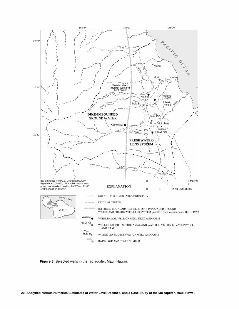
20 Analytical Versus Numerical Estimates of Water-Level Declines, and a Case Study of the Iao Aquifer, Maui, Hawaii
P AC
I FI C
OC
EA
N
Iao-Waikapu Ditch
Waihee
Spreckels
Di tc h
Ditch
Maniania
Ditc
h
NorthWaiehu Stream
SouthWaiehu Str ea
m
Wai
ehu
Stream
Iao
Stre
am
20o54'
20o52'
20o56'
156o30'156o32'156o34'
Waihee
Waiehu
Wailuku
Waikapu
0
0
2 MILES1
1 2 KILOMETERSEXPLANATION
IAO AQUIFER STUDY-AREA BOUNDARY
DITCH OR TUNNEL
INFERRED BOUNDARY BETWEEN DIKE-IMPOUNDED GROUNDWATER AND FRESHWATER-LENS SYSTEM (modified from Yamanaga and Huxel, 1970)
WITHDRAWAL WELL OR WELL FIELD AND NAME
WELL FIELD WITH WITHDRAWAL AND WATER-LEVEL OBSERVATION WELLS AND NAME
WATER-LEVEL OBSERVATION WELL AND NAME
RAIN GAGE AND STATE NUMBER
DIKE-IMPOUNDEDGROUND WATER
FRESHWATER-LENS SYSTEM
MAUI
Areaof map
Pacific Ocean
Test hole E
Test hole 15D
Test hole B
Waiehu deep monitor well and
Test hole D
484
484
Test hole B
Shaft 33
Shaft 33
Mokuhau
Waihee
Waihee WaiehuHeights
Kepaniwai
Base modified from U.S. Geological Surveydigital data, 1:24,000, 1983, Albers equal area projection, standard parallels 20°35' and 21°00', central meridian 156°20'
Figure 8. Selected wells in the Iao aquifer, Maui, Hawaii.

Case Study of the Iao Aquifer, Maui 21
0
0
2 MILES1
1 2 KILOMETERS
P AC
I FI C
OC
EA
N
WaiheeWaihee
WailukuWailukuWailuku
WaikapuWaikapu
PuuPuuKukuiPuu
Kukui
Waiehu
Waikapu
EXPLANATION
SEDIMENTARY DEPOSITS
Unconsolidated deposits, chiefly younger alluvium
Calcareous sand dunes
Consolidated earthy deposits, chiefly older alluvium
VOLCANIC ROCKS
Honolua Volcanics
Wailuku Basalt
CONES, VENTS, DOMES, CRATERS, BOSSES, AND DIKES
Cones or domes of Honolua Volcanics
Pit craters
Bosses of Wailuku Basalt
Dikes of either Wailuku Basalt or Honolua Volcanics
Dikes, where too numerous to show individually
Axis of rift zone (from Macdonald and others, 1983)
Caldera boundary, dotted where concealed, dashed where inferred
INFERRED BOUNDARY BETWEEN-DIKE IMPOUNDED GROUND WATER AND FRESHWATER-LENS SYSTEM
STUDY-AREA BOUNDARY
Base modified from U.S. Geological Surveydigital data, 1:24,000, 1983, Albers equal area projection, standard parallels 20°35' and 21°00', central meridian 156°20'
156°34'
21°56'
21°54'
21°52'
156°30'156°32'
Figure 9. Surficial geology of the Iao aquifer area, Maui, Hawaii (modified from Stearns and Macdonald, 1942 andLangenheim and Clague, 1987).

22 Analytical Versus Numerical Estimates of Water-Level Declines, and a Case Study of the Iao Aquifer, Maui, Hawaii
Water-level data of most interest for this discus-sion are from the 1990’s, when total withdrawalincreased and reached (in 1995 and 1996) the sustain-able-yield value used by CWRM. Water levels nearshaft 33 were measured intermittently from 1940through 1970. After 1970, water levels were not mea-sured until 1996 when measurements were made in oneof the unused wells at shaft 33 (fig. 10). Water levels atand near Mokuhau well field were measured from 1951to 1979. After 1979, water levels were not measureduntil 1998 when measurements were made in one of theunused wells in the Mokuhau well field (fig. 11) (Meyerand Presley, 2000). Water levels near Waihee andWaiehu Heights well fields can be inferred from water-level measurements made at the nearby Waiehu deepmonitor well and at test holes B, D, and E (fig. 12)(Meyer and Presley, 2000). Given their locations (fig.8), water levels in the Waiehu deep monitor well andtest holes B and D can be considered representative ofwater levels at Waihee well field, and water levels attest holes B and E can be considered representative ofthose at Waiehu Heights well field.
Changes in water levels in observation wells in thearea of Waiehu Heights and Waihee well fields indicatethat water levels in the Iao aquifer respond to changesin withdrawals, rainfall, and recharge from irrigation.Between April 1977 and April 1997, water levelsdeclined by about 6 ft near these wells (from about 15to 16 ft above sea level in April 1977 to about 9 to 10 ftabove sea level in April 1997) (fig. 13). During thisperiod, withdrawals from the Waiehu Heights andWaihee well fields increased and recharge from irriga-tion decreased. Withdrawals at the Waiehu Heights andWaihee well fields started in 1977 and 1979, respec-
tively. In addition, because of changes in irrigationpractices, changes in types of crops grown, and reduc-tion in agricultural acreage, estimated recharge fromirrigation decreased from 17 Mgal/d during 1926–79, to6 Mgal/d during 1980–85, to 2 Mgal/d during 1986–95(Shade, 1997). The water-level declines (fig. 12) werenot continuous, however, indicating that water levelsare influenced by a factor or factors in addition toincreased withdrawals from the Waiehu Heights andWaihee well fields and decreased recharge from irriga-tion. During the 1980’s, water levels rose above 1977and 1979 water levels because of reduced withdrawalsfrom the Mokuhau well field and shaft 33 and variationsin rainfall. Between 1977 and 1991, trends in water lev-els in the vicinity of the two well fields correlate closelyto the 12-month departure of rainfall from mean rainfall(Meyer and Presley, 2000) (fig. 12). From 1992onward, however, there is little correlation betweenrainfall and water levels. Average water levels declinedfrom 1990 through 1996, in apparent response toincreased withdrawals from the aquifer between 1990and 1996. Although withdrawal was reduced in 1997,water levels continued to decline through 1997. Furtherreduction of withdrawal in 1998 resulted in a slightincrease in water levels. Changes in rainfall would beexpected to affect water levels, but the effect of with-drawal on water levels is more significant than theeffect of recent (1990–98) changes in rainfall. Average1998 water levels are about 10 ft above sea level at allof the well fields.
The RAM-predicted equilibrium heads,he, associ-ated with the 20 Mgal/d value of sustainable yield usedby CWRM can be determined in two ways: (1) by using
aWell also used for vertical salinity-profile information.
Table 4. State numbers and names of selected wells in the Iao aquifer, Maui, Hawaii
State wellnumber Well name Use of well
5330-05 Shaft 33 withdrawal and water-level observation5330-07 Test hole 15D water-level observation5330-09 to -11 Mokuhau withdrawal and water-level observation5332-05 Kepaniwai withdrawal5430-01, -02 Waiehu Heights withdrawal5430-03 Test hole E water-level observation5430-04 Test hole D water-level observation5430-05 Waiehu deep monitor water-level observationa
5431-01 Test hole B water-level observation5431-02 to -04 Waihee withdrawal

Case Study of the Iao Aquifer, Maui 23
Table 5. Annual ground-water withdrawal from the Iao aquifer, Maui, Hawaii[Values in million gallons per day, or percentage where noted; --, not applicable; data from Maui Department of Water Supply and unpublished data fromWailuku Sugar Co. in U.S. Geological Survey well files, Honolulu]
Well fieldDomestic
(percentageof total)Year
WaiehuHeights Waihee Kepaniwai Mokuhau Shaft 33 Total Domestic
1948 -- -- -- -- 2.00 2.00 0.00 0.01949 -- -- -- -- 1.99 1.99 0.00 0.01950 -- -- -- -- 1.77 1.77 0.00 0.01951 -- -- -- -- 3.70 3.70 0.00 0.01952 -- -- -- -- 3.05 3.05 0.00 0.01953 -- -- -- -- 9.77 9.77 0.00 0.01954 -- -- -- -- 6.11 6.11 0.00 0.01955 -- -- -- 1.10 1.31 2.41 1.10 45.61956 -- -- -- 0.66 0.83 1.49 0.66 44.31957 -- -- -- 1.19 6.12 7.31 1.19 16.31958 -- -- -- 1.22 0.67 1.89 1.22 64.61959 -- -- -- 1.43 4.15 5.58 1.43 25.61960 -- -- -- 1.59 5.65 7.24 1.59 22.01961 -- -- -- 2.25 5.64 7.89 2.25 28.51962 -- -- -- 2.04 7.97 10.01 2.04 20.41963 -- -- -- 2.06 0.85 2.91 2.06 70.81964 -- -- -- 2.79 6.00 8.79 2.79 31.71965 -- -- -- 2.67 4.68 7.35 2.67 36.31966 -- -- -- 3.12 4.69 7.81 3.12 39.91967 -- -- -- 2.91 3.08 5.99 2.91 48.61968 -- -- -- 2.88 6.28 9.16 2.88 31.41969 -- -- -- 3.61 1.18 4.79 3.61 75.41970 -- -- -- 3.98 5.08 9.06 3.98 43.91971 -- -- -- 4.34 11.65 15.99 4.34 27.11972 -- -- -- 4.66 9.45 14.11 4.66 33.01973 -- -- -- 5.16 8.11 13.27 5.16 38.91974 -- -- -- 5.44 9.11 14.55 5.44 37.41975 -- -- -- 6.40 10.56 16.96 6.40 37.71976 -- -- -- 6.69 6.37 13.06 6.69 51.21977 0.38 -- 0.04 8.10 6.39 14.91 8.52 57.11978 0.46 -- 0.01 8.29 3.14 11.90 8.76 73.61979 0.48 1.37 0.02 6.51 3.29 11.67 8.38 71.81980 0.48 6.15 0.02 3.05 0.00 9.70 9.70 100.01981 0.59 4.87 0.03 5.80 1.18 12.47 11.29 90.51982 0.49 5.20 0.007 4.60 0.00 10.30 10.30 100.01983 0.34 5.39 0.14 5.82 0.00 11.69 11.69 100.01984 0.29 5.41 0.11 6.39 0.37 12.57 12.20 97.11985 0.18 5.12 0.03 6.52 0.00 11.85 11.85 100.01986 0.27 6.63 0.003 6.42 0.00 13.32 13.32 100.01987 0.34 8.53 0.003 5.11 0.00 13.98 13.98 100.01988 0.35 8.06 0.00 6.71 0.00 15.12 15.12 100.01989 0.51 7.34 0.00 7.49 0.00 15.34 15.34 100.01990 0.92 8.66 0.07 7.66 0.00 17.31 17.31 100.01991 1.96 8.22 1.03 5.72 1.90 18.83 18.83 100.01992 1.08 7.96 0.82 3.17 5.10 18.13 18.13 100.01993 1.51 7.24 0.49 3.60 5.56 18.40 18.40 100.01994 1.20 8.15 0.45 6.49 2.91 19.20 19.20 100.01995 1.71 7.92 0.49 4.92 5.46 20.50 20.50 100.01996 1.56 8.22 0.28 5.13 5.16 20.35 20.35 100.01997 1.23 8.94 0.80 6.29 1.84 19.10 19.10 100.01998 0.23 9.11 0.51 3.21 4.84 17.90 17.90 100.0

24 Analytical Versus Numerical Estimates of Water-Level Declines, and a Case Study of the Iao Aquifer, Maui, Hawaii
J F M A M J J A S O N D J F M A M J J A S O N D J F M A M J J A S O N D1996 1997 1998
8
18
9
10
11
12
13
14
15
16
17
MO
NT
HLY
ME
AN
WA
TE
R L
EV
EL,
IN F
EE
T A
BO
VE
ME
AN
SE
A L
EV
EL
RAM-predicted equilibrium head, he = 14 ft (assuming he:h0 ratio of 0.5 from table 1)
RAM-predicted equilibrium head, he = 17 ft (assuming he:h0 ratio of 0.6 from equation 3)
5
30
10
15
20
25
WA
TE
R L
EV
EL,
IN F
EE
T A
BO
VE
ME
AN
SE
A L
EV
EL
1950 1952 1954 1956 1958 1960 1962 1964 1966 1968 1970 1972 1974 1976 1978 1980 1982 1984 1986 1988 1990 1992 1994 1996 1998 2000
Pumps 1 (5330-10) and 2 (5330-09)
Pump 2 (5330-09)
Test hole 15D (5330-07)
RAM-predicted equilibrium head, he = 14 ft
Figure 11. Water levels at Mokuhau well field, Iao aquifer, Maui, Hawaii.
Figure 10. Water levels at shaft 33 during 1996–98, Iao aquifer, Maui, Hawaii.

Case Study of the Iao Aquifer, Maui 25
DE
PA
RT
UR
E O
F 1
2-M
ON
TH
MO
VIN
G A
VE
RA
GE
RA
INF
ALL
, IN
PE
RC
EN
T
MO
NT
HLY
WIT
HD
RA
WA
L,IN
MIL
LIO
N G
ALL
ON
SP
ER
DA
Y
-100
150
-50
0
50
100
0
28
4
8
12
16
20
24
1976 1978 1980 1982 1984 1986 1988 1990 1992 1994 1996 1998 2000
Test hole B (5431-01)
Test hole D (5430-04) and Waiehu deep monitor well (5430-05)
Test hole E (5430-03)
Iao aquifer withdrawal
Waiehu Camp (station 484)
WA
TE
R L
EV
EL,
IN F
EE
T A
BO
VE
ME
AN
SE
A L
EV
EL minimum water level 7.84 ft measured October 1996
minimum water level 9.65 ft measured October 1996
minimum water level 9.01 ft measured October 1996
RAM-predicted equilibrium head, he = 15 ft
RAM-predicted equilibrium head, he = 15 ft
RAM-predicted equilibrium head, he = 15 ft
24
8
12
16
20
22
6
10
14
18
22
6
10
14
18
Figure 12. Water levels at Waiehu deep monitor well and test holes B and E, departure of back-ward-looking 12-month moving average rainfall from the long-term average rainfall for WaiehuCamp rain gage, and monthly mean total withdrawal from the Iao aquifer prior to 1999, Maui,Hawaii. (Unpublished rainfall data from Commission on Water Resource Management.)

26 Analytical Versus Numerical Estimates of Water-Level Declines, and a Case Study of the Iao Aquifer, Maui, Hawaii
P AC
I FI C
OC
EA
N
??
??
?
??
?
??
2 W
aiehu Stream
Iao
Stre
am
Waihee
Waiehu
Wailuku
Waikapu
0
0
1 MILE
1 KILOMETER
DIKE-IMPOUNDED
GROUNDWATER FRESHWATER-LENS
SYSTEM
AREA UNDERLAIN BY CONFINED FRESH GROUND WATER IN THE WAILUKU BASALT
LINE OF EQUAL WATER-LEVEL DECLINE--Contour interval is one foot. Dashed where appoximately located. Datum is mean sea level.
APPROXIMATE SEAWARD EXTENT OF FRESHWATER IN WAILUKU BASALT FOR PREDEVELOPMENT CONDITIONS
BOUNDARY BETWEEN UNCONFINED AND CONFINED WATER IN THE WAILUKU BASALT
INFERRED BOUNDARY BETWEEN DIKE-IMPOUNDED GROUND WATER AND FRESHWATER-LENS SYSTEM (modified from Yamanaga and Huxel, 1970)
STUDY-AREA (IAO AQUIFER) BOUNDARY
WITHDRAWAL WELL OR WELL FIELD AND NAME
WELL FIELD WITH WITHDRAWAL AND WATER-LEVEL OBSERVATION WELLS AND NAME
WATER-LEVEL OBSERVATION WELL AND NAME
EXPLANATION
KahuluiBay
20°56'
20°54'
20°52'
156°32' 156°30'
WaiheeWaiehuHeights
Kepaniwai
Test hole E
Test hole15D
Test hole B
Waiehu deep monitor well
and Test hole D
Shaft 33
Waihee
Test hole B
Shaft 33
Mokuhau
2
3
4
5 6
2
3
4
5 6
Base modified from U.S. Geological Surveydigital data, 1:24,000, 1983, Albers equal area projection, standard parallels 20°35' and 21°00', central meridian 156°20'
Waihee River
Waikapu Stream
MAUI
Areaof map
Pacific Ocean
Figure 13. Map showing water-level declines in the flank flows of Wailuku Basalt between April 1977 and April 1997for the northern part of the Iao aquifer, Maui, Hawaii.

Case Study of the Iao Aquifer, Maui 27
equation 3, or (2) by using ratios ofhe:h0 from table 1.Using equation 3 and assumingD andI values of 20Mgal/d and 31.57 Mgal/d (Mink, 1995), respectively,the ratiohe:h0 is computed to be 0.6 for the Iao aquifer.Predevelopment heads averaged 28.5 ft above sea levelnear shaft 33 and 24 ft above sea level near the Moku-hau well field. Thus, using a ratio forhe:h0 of 0.6, theRAM-predicted equilibrium heads are about 17 ft and14 ft for the shaft 33 and Mokuhau well fields, respec-tively (table 6). No information exists for predevelop-ment heads at the Waiehu Heights and Waihee wellfields, although Yamanaga and Huxel (1970) suggestthat they might have been about 25 ft above sea level.For a predevelopment head of 25 ft above sea level, anda ratio ofhe:h0 of 0.6, the RAM-predicted equilibriumhead for the Waiehu Heights and Waihee well fields is15 ft above sea level.
For a predevelopment head of 28.5 ft above sealevel at shaft 33, the ratio ofhe:h0 from table 1 is 0.5.Thus, on the basis of ratios ofhe:h0 from table 1, theequilibrium head for shaft 33 is estimated to be about 14ft, which is lower than the 17-ft value previously calcu-lated using equation 3. At the Mokuhau, WaiehuHeights, and Waihee well fields, predevelopment headsranged from about 24 to 25 ft above sea level. Thus, theratio ofhe:h0 from table 1 for these well sites is 0.6,which is the same value calculated using equation 3.
In 1995 and 1996, withdrawal from the Iao aquiferreached the sustainable-yield value derived usingRAM. However, by 1996 or earlier, water levels at shaft33 and Waiehu Heights (represented with water levelsfrom test holes B and E) were below RAM-predictedequilibrium heads. Water levels at Waihee well field(represented with water levels from the Waiehu deepmonitor well and test hole B) also were below theRAM-predicted equilibrium head and were at an alti-tude that potentially could have resulted in saltwaterintrusion. No water-level data were available for Moku-hau well field in 1996. CWRM held hearings on the sta-tus of the aquifer and in April 1997 concluded that“current pumpage rates in current locations cannot besustained in the long term” (State of Hawaii, 1997, p. 4).
Although the decline in water levels ceased prior to1999, average 1998 water levels were still below RAM-predicted equilibrium heads for shaft 33, Mokuhau,Waihee, and Waiehu Heights well fields. At their low-est altitudes prior to 1999, water levels were 5 to 7 ft
below RAM-predicted equilibrium heads for Waiheeand Waiehu Heights well fields, and about 5 ft belowthe 14-ft RAM-predicted equilibrium head for shaft 33.Water-level data for Mokuhau well field were not avail-able until 1998 when the average water level was about4 ft below the RAM-predicted equilibrium head for thiswell field (table 6).
Water levels in the Iao aquifer continued to declinewhen withdrawal was at the sustainable-yield valuedetermined from RAM. The ultimate decline that wouldhave occurred if withdrawal was permitted to remain at20 Mgal/d cannot be estimated from available data. Therise in the position of the brackish-water transition zonegenerally will not occur immediately following adecline in water level. Rather, the change in position ofthe transition zone will generally lag behind the changein water level (see, for example, Essaid, 1986). Thus,the ultimate rise in the transition zone that would haveoccurred if withdrawal was permitted to remain at 20Mgal/d also cannot be estimated from available data.However, even with average 1998 withdrawal at about18 Mgal/d, water levels were probably still belowacceptable long-term values to preclude saltwater intru-sion at some of the well fields (Meyer and Presley,2000).
Although uncertainty associated with the rechargeestimate and predevelopment water levels contributesto uncertainty in the equilibrium heads predicted byRAM, the decline of water levels below those predictedby RAM in the vicinity of the well fields in the Iao aqui-fer is consistent with the results of the preceding numer-ical model analysis that demonstrate (1) the effect of acaprock on water-level declines caused by withdrawals,and (2) the importance of representing the distributionof withdrawals in an aquifer. The field setting for theIao aquifer is similar to that shown in figure 7, andalthough the model does not simulate the Iao aquifer,model results provide insight to why water levels in theIao aquifer fell below equilibrium heads predicted byRAM. Water availability in the Iao aquifer can be bestunderstood by constructing a numerical model of theground-water flow system. The data needs, requiredexpertise, and development time are much greater forconstructing a numerical model than for using RAM.Although construction of a numerical model is morecostly than simply using RAM, a numerical model willlead to an improved understanding of the ground-watersystem and better management decisions.
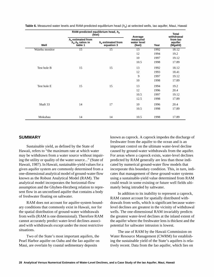
28 Analytical Versus Numerical Estimates of Water-Level Declines, and a Case Study of the Iao Aquifer, Maui, Hawaii
SUMMARY
Sustainable yield, as defined by the State ofHawaii, refers to “the maximum rate at which watermay be withdrawn from a water source without impair-ing the utility or quality of the water source...” (State ofHawaii, 1987). In Hawaii, sustainable-yield values for agiven aquifer system are commonly determined from aone-dimensional analytical model of ground-water flowknown as the Robust Analytical Model (RAM). Theanalytical model incorporates the horizontal-flowassumption and the Ghyben-Herzberg relation to repre-sent flow in an unconfined aquifer that contains a bodyof freshwater floating on saltwater.
RAM does not account for aquifer-system bound-ary conditions that commonly exist in Hawaii, nor forthe spatial distribution of ground-water withdrawalsfrom wells (RAM is one dimensional). Therefore RAMcannot accurately predict water-level declines associ-ated with withdrawals except under the most restrictivesituations.
Two of the State’s most important aquifers, thePearl Harbor aquifer on Oahu and the Iao aquifer onMaui, are overlain by coastal sedimentary deposits
known as caprock. A caprock impedes the discharge offreshwater from the aquifer to the ocean and is animportant control on the ultimate water-level declinecaused by ground-water withdrawals from the aquifer.For areas where a caprock exists, water-level declinespredicted by RAM generally are less than those indi-cated by numerical ground-water flow models thatincorporate this boundary condition. This, in turn, indi-cates that management of these ground-water systemsusing a sustainable-yield value determined from RAMcould result in some existing or future well fields ulti-mately being intruded by saltwater.
In addition to its inability to represent a caprock,RAM cannot account for spatially distributed with-drawals from wells, which is significant because water-level declines are greatest in the vicinity of withdrawalwells. The one-dimensional RAM invariably predictsthe greatest water-level declines at the inland extent ofthe aquifer where the freshwater lens is thickest and thepotential for saltwater intrusion is lowest.
The use of RAM by the Hawaii Commission onWater Resource Management (CWRM) for establish-ing the sustainable yield of the State’s aquifers is rela-tively recent. Data from the Iao aquifer, which lies on
Table 6. Measured water levels and RAM-predicted equilibrium head (he) at selected wells, Iao aquifer, Maui, Hawaii
RAM-predicted equilibrium head, he(feet)
Averagemeasuredwater level
(feet)
Totalwithdrawal
from Iaoaquifer(Mgal/d)Well
he estimated fromhe:h0 ratios in
table 1he estimated from
equation 3 Year
Waiehu monitor 15 15 13 1992 18.1212 1994 19.210 1997 19.1210.5 1998 17.89
Test hole B 15 15 13 1992 18.1212 1993 18.419 1997 19.12
10 1998 17.89
Test hole E 15 15 13 1994 19.212 1996 20.410.5 1997 19.1212.5 1998 17.89
Shaft 33 14 17 10 1996 20.410.5 1998 17.89
Mokuhau 14 14 10.5 1998 17.89

References Cited 29
the northeastern flank of the West Maui Volcano andwhich is confined near the coast by a caprock, are nowavailable to evaluate the predictive capability of RAMfor this aquifer. In 1995 and 1996, withdrawal reachedthe sustainable-yield value derived using RAM (State ofHawaii, 1990). However, even before 1996, water lev-els in the aquifer had declined significantly below thosepredicted by RAM and were still declining in 1997. Asa result, it was necessary to reduce withdrawal from theaquifer below the sustainable-yield value derived usingRAM in order to halt the continuing decline of waterlevels and to preclude the ultimate intrusion of saltwaterinto the four major well fields in the aquifer.
Although uncertainty associated with the rechargeestimate and predevelopment water levels contributesto uncertainty in the equilibrium heads predicted byRAM, the decline of water levels below those predictedby RAM in the Iao aquifer is consistent with the resultsof the numerical model analysis that demonstrate (1) theeffect of a caprock on water-level declines caused bywithdrawals, and (2) the importance of representing thedistribution of withdrawals in an aquifer. Water avail-ability in the Iao aquifer can be best understood by con-structing a numerical model of the ground-water flowsystem.
REFERENCES CITED
Bear, Jacob, 1972, Dynamics of fluids in porous media: NewYork, American Elsevier, 764 p.
Bredehoeft, J.D., Papadopulous, S.S., and Cooper, H.H.,1982, Groundwater: the water-budget myth,in U.S.National Research Council, Scientific basis of water-resource management: Washington, D.C., NationalAcademy Press, p. 51–57.
Bredehoeft, J.D., and Hall, Phil, 1995, Ground-water models:Ground Water, v. 33, no. 4., p. 530–531.
Domenico, P.A., and Schwartz, F.W., 1990, Physical andchemical hydrogeology, New York, John Wiley & Sons,Inc., 824 p.
Essaid, H.I., 1986, A comparison of the coupled fresh water-salt water flow and the Ghyben-Herzberg sharp interfaceapproaches to modeling of transient behavior in coastalaquifer systems: Journal of Hydrology, v. 86, no. 1/2,p. 169–193.
Essaid, H.I., 1990, The computer model SHARP, a quasi-three-dimensional finite-difference model to simulatefreshwater and saltwater flow in layered coastal aquifer
systems: U.S. Geological Survey Water-ResourcesInvestigations Report 90-4130, 181 p.
Eyre, Paul, Ewart, Charles, and Shade, Patricia, 1986,Hydrology of the leeward aquifers, southeast Oahu,Hawaii: U.S. Geological Survey Water-Resources Inves-tigations Report 85-4270, 75 p.
Giambelluca, T.W., 1986, Land-use effects on the water bal-ance of a tropical island: National Geographic Research,v. 2, no. 2, p. 125–151.
Gingerich, S.B., 1998, Numerical modelling of verticallyextensive groundwater bodies in Maui, Hawaii: an alter-native to perched aquifers: International Association ofHydrological Sciences Publication no. 253, p. 167–174.
Gingerich, S.B., 1999, Estimating transmissivity and storageproperties from aquifer tests in the Southern LihueBasin, Kauai, Hawaii: U.S. Geological Survey Water-Resources Investigations Report 99-4066, 33 p.
Hunt, C.D., Jr., 1996, Geohydrology of the island of Oahu,Hawaii: U.S. Geological Survey Professional Paper1412-B, 54 p.
Izuka, S.K., and Gingerich, S.B., 1998, Ground water in theSouthern Lihue Basin, Kauai, Hawaii: U.S. GeologicalSurvey Water-Resources Investigations Report 98-4031,71 p.
Langenheim, V.A.M., and Clague, D.A., 1987, The Hawai-ian-Emperor volcanic chain, part II, stratigraphic frame-work of volcanic rocks of the Hawaiian Islands, chap. 1of Decker, R.W., Wright, T.L., and Stauffer, P.H., eds.,Volcanism in Hawaii: U.S. Geological Survey Profes-sional Paper 1350, v. 1, p. 55–84.
Macdonald, G.A., Abbott, A.T., and Peterson, F.L., 1983,Volcanoes in the sea: The geology of Hawaii (2d ed.):Honolulu, Hawaii, University of Hawaii Press, 517 p.
Meyer, William, and Presley, T.K., 2000, The response of theIao aquifer to ground-water development, rainfall, andland-use practices between 1940 and 1998, island ofMaui, Hawaii: U.S. Geological Survey Water-ResourcesInvestigations Report 00-4223, 60 p.
Mink, J.F., 1980, State of the groundwater resources of south-ern Oahu, Honolulu Board of Water Supply, 83 p.
Mink, J.F., Yuen, G.A.L., and Chang, J.Y.C., 1988, Reviewand re-evaluation of groundwater conditions in the PearlHarbor groundwater control area Oahu, Hawaii: State ofHawaii Department of Land and Natural Resources,Report R-78, 95 p. plus appendixes.
Mink, J.F., 1995, Sustainable yields, Maui and Molokai: let-ter dated September 9, 1995 to Rae M. Loui, State ofHawaii Commission on Water Resource Management,2 p.
Oki, D.S., 1997, Geohydrology and numerical simulation ofthe ground-water flow system of Molokai, Hawaii: U.S.

30 Analytical Versus Numerical Estimates of Water-Level Declines, and a Case Study of the Iao Aquifer, Maui, Hawaii
Geological Survey Water-Resources InvestigationsReport 97-4176, 62 p.
Oki, D.S., 1998, Geohydrology of the central Oahu, Hawaii,ground-water flow system and numerical simulation ofthe effects of additional pumping: U.S. Geological Sur-vey Water-Resources Investigations Report 97-4276,132 p.
Oki, D.S., 1999, Geohydrology and numerical simulation ofthe ground-water flow system of Kona, island of Hawaii:U.S. Geological Survey Water-Resources InvestigationsReport 99-4073, 70 p.
Oki, D.S., Tribble, G.W., Souza, W.R., and Bolke, E.L.,1999, Ground-water resources in Kaloko-HonokohauNational Historical Park, island of Hawaii, Hawaii, andnumerical simulation of the effects of ground-waterwithdrawals: U.S. Geological Survey Water-ResourcesInvestigations Report 99-4070, 49 p.
Shade, P.J., 1997, Water budget for the Iao area, island ofMaui, Hawaii: U.S. Geological Survey Water-ResourcesInvestigations Report 97-4244, 25 p.
Souza, W.R., and Voss, C.I., 1987, Analysis of an anisotropiccoastal aquifer system using variable-density flow andsolute transport simulation: Journal of Hydrology, v. 92,p. 17–41.
State of Hawaii, 1987, State water code: Hawaii Revised Stat-utes, Chapter 174C.
State of Hawaii, 1990, Water resources protection plan, vol-umes I and II, June 1990: Commission on WaterResource Management, Department of Land and NaturalResources, variously paged.
State of Hawaii, 1992, Water resources protection plan, vol-umes I and II, review draft, March 1992: Commission onWater Resource Management, Department of Land andNatural Resources, 313 p. plus appendixes.
State of Hawaii, 1997, Recommendation on the designationof the Iao aquifer system as a ground water managementarea: Staff submittal for the meeting of the Commissionon Water Resource Management, April 16, 1997,Wailuku, Maui, 7 p. plus exhibits.
Stearns, H.T., and Macdonald, G.A., 1942, Geology andground-water resources of the island of Maui, Hawaii:Hawaii Division of Hydrography Bulletin 7, 344 p.
Underwood, M.R., Meyer, William, and Souza, W.R., 1995,Ground-water availability from the Hawi aquifer in theKohala area, Hawaii: U.S. Geological Survey Water-Resources Investigations Report 95-4113, 57 p.
Yamanaga, George, and Huxel, C.J., Jr., 1970, Preliminaryreport on the water resources of the Wailuku area, Maui:State of Hawaii Department of Land and NaturalResources, Division of Water and Land Development,Circular C61, 43 p.
APPENDIX: DESCRIPTION OF RAM
The one-dimensional Robust Analytical Model(RAM) (Mink, 1980) used by CWRM to estimate sus-tainable yield incorporates the Dupuit assumption ofhorizontal flow (see, for example, Bear, 1972) and theGhyben-Herzberg relation. The steady-state model isdescribed and derived in this appendix.
Dupuit Assumption
For ground-water flow systems with small water-table slopes, an approximate solution for flow in anunconfined aquifer can be derived. The assumption ofsmall water-table slope is equivalent to assuming thatequipotential surfaces are vertical and flow is essen-tially horizontal, or to assuming that a hydrostatic pres-sure distribution exists (Bear, 1972, p. 361). This isknown as the Dupuit assumption. With the Dupuitassumption, variations in velocity and pressure in thevertical direction are neglected and, thus, two-dimen-sional flow in a vertical cross section can be approxi-mated by one-dimensional flow in the horizontaldirection.
In general, ground-water flow in an unconfinedaquifer is three dimensional. If ground-water flow isfirst assumed to be adequately represented by flow in atwo-dimensional vertical cross section, and if the hori-zontal-flow assumption is then used, the original three-dimensional flow system can be approximated by a one-dimensional system.
Ghyben-Herzberg Relation
In Hawaii, fresh ground water commonly occurs asa lens-shaped body of freshwater floating on denser,underlying saltwater derived from the ocean. A brack-ish-water transition zone of varying thickness existsbetween the freshwater and underlying saltwater. Thetransition zone is created by mixing of saltwater withseaward flowing freshwater.
For areas where the brackish-water transition zoneis thin, the Ghyben-Herzberg relation can be used toestimate the thickness of the freshwater lens. If the spe-cific gravities of freshwater and saltwater are assumedto be 1.000 and 1.025, respectively, then the Ghyben-Herzberg relation predicts that every foot of freshwaterabove sea level must be balanced by 40 ft of freshwaterbelow sea level. The Ghyben-Herzberg relation is valid
Appendix: Description of RAM 31
for hydrostatic conditions. For dynamic conditions, theGhyben-Herzberg relation tends to underestimate fresh-water-lens thickness near the discharge zone and over-estimate lens thickness near the recharge zone.
One-Dimensional Analytical Equation
The flow rate in a porous medium is proportionalto the cross-sectional area of flow and the hydraulic gra-dient, and can be described by Darcy’s law. For one-dimensional steady-state flow, Darcy’s law can be writ-ten as:
Q = –K i A, (a1)
where, Q = rate of flow [L3/T],K = hydraulic conductivity [L/T],i = hydraulic gradient [L/L], and
A = cross-sectional area of flow [L2].The constant of proportionality in Darcy’s law is
the hydraulic conductivity,K, which is related to theproperties of the porous medium and the fluid. Thehydraulic conductivity is a quantitative measure of thecapacity of a rock to transmit water. For one-dimen-sional flow, the hydraulic gradient is given by:
i = dh/dx,
where, h = hydraulic head [L] measured relative tomean sea level,
x = Cartesian coordinate [L], anddh/dx = derivative ofh with respect tox.
Flow is in the direction of decreasing hydraulichead, which accounts for the negative sign in equationa1. The cross-sectional area of flow at any section isgiven by:
A = 41hw,
where, w = width of section [L], and41h = height of section from the Ghyben-
Herzberg relation [L].
Thus, Darcy’s law can be expressed as:
Q = –K (dh/dx) (41hw). (a2)
Rearranging terms yields:
–[Q/(41Kw)] dx = h dh. (a3)
Integration of equation (a3) yields:
–[Q/(41Kw)] (x2–x1) = 0.5(h22 – h1
2). (a4)
If h1 = 0 atx1 = 0, then from equation (a4),h as afunction ofx can be written as:
h2 = –[2Q/(41Kw)] x. (a5)
Equation (a5) forms the basis of RAM. Equation(a5) can be rearranged as:
h2/Q = –2x/(41Kw). (a6)
For any given location,x, the right hand side ofequation (a6) is a constant and, thus, the ratio ofh2/Q isa constant:
h02/Q0 = he
2/Qe, (a7)
where, h0 = hydraulic head [L] at locationx forflow rateQ0,
Q0 = steady-state rate of flow throughaquifer for predevelopmentconditions [L3/T],
he = hydraulic head [L] at locationx forflow rateQe, and
Qe = steady-state rate of flow (lesswithdrawals from wells or shafts)through aquifer for developmentconditions [L3/T].
For some desired equilibrium head,he, CWRMdefines the sustainable yield,D, as the differencebetween the predevelopment rate of flow through theaquifer minus the reduced rate of flow through the aqui-fer following development:
D = Q0 − Qe. (a8)
Combining equations (a7) and (a8), and lettingQ0 = I yields:
D/I = 1− (he/h0)2. (a9)
Equation (a9) represents the model (RAM) used byCWRM to set sustainable yield in Hawaii. To apply thisequation, predevelopment values forh0 andI must beknown. After establishing some desired minimum equi-librium head,he, equation (a9) is used by CWRM toestimate the sustainable yield of an aquifer. For exam-ple, if the desired equilibrium head is 60 percent of thepredevelopment head (he/h0 = 0.6), thenD/I = 1 –(0.6)2, orD/I = 0.64. Thus, RAM estimates that thesustainable yield,D, is 64 percent of the predevelop-ment flow rate,I, in the aquifer for this case.