KEYNOTE ADDRESS 1

ANALYTICAL TOOLS FOR DESIGN OF FLEXIBLE PAVEMENTSDr. Per Ullidtz, Technical University of Denmark

Abstract: This paper falls into two parts. In the first, the widely used analytical-empirical method of pavementdesign and evaluation is discussed and in the second two simulation models are presented. There are importantdifferences between the assumptions on which the theoretical models are based, and the reality of pavementmaterials and structures, and these differences are important both for the determination of input values(elastic parameters) and for the calculation of pavement response. Linear elastic theory often results in incor-rect moduli, when used for backcalculation of layer moduli from deflection testing, and in questionablestresses and strains, when used for forward calculation. Including non-linear materials characteristics mayimprove the theoretical model, but no theoretical model has yet been conclusively verified with experimentaldata. The empirical relationships used to predict pavement deterioration from critical stresses or strains, areequally problematic.In the second part of the paper two theoretical models are presented. The first model simulates the dete-rioration of a section of pavement over time using an incremental-recursive process. The model is stochasticand considers the spatial variation of pavement materials, layer thickness and traffic loads as well as seasonalvariations. The second model deals with the forces on, and the displacements of, the individual grains in aparticulate medium. This model does not rely on empirical relationships to predict permanent deformationor failure, but models this in the same process as forces and displacements. The input to this model includesthe grain size distribution, the shape of the grains and the degree of compaction, parameters that are similarto those used for specification of materials and quality control.It is concluded that an interaction between development of theoretical models and experimental verificationis needed to improve the understanding and predictability of the complex process of pavement deterioration.

1. Introduction, the Analytical-Empirical MethodProfessor S.F. Brown in his keynote address to the 8th International conference on Asphalt Pavements inSeattle in 1997 (Brown, 1997) gave an excellent description of the importance of the “Ann Arbor” conferencesfor the transition of structural design of asphalt pavements away from purely empirical methods toward amore analytical (or mechanistic) approach, similar to the approaches used for other engineering structures.

The Analytical-Empirical (or Mechanistic-Empirical) approach to design of flexible pavements has two steps,as implied by the name. In the first step the critical stresses or strains (the response) in the individual pavementlayers are calculated using an analytical model, and in the second step they are compared to permissiblestresses or strains. In the more sophisticated versions, the critical stresses or strains are used for determiningthe rate of deterioration (the performance).

Figure 1Pavement response (analytical) and performance (empirical)

There is not a strict limit between the analytical and the empirical part of the method. If an equivalentstandard axle is used with a mean annual pavement condition, the effects of real traffic loading and seasonal

2 KEYNOTE ADDRESS

variations, will be included in the empirical part. The tendency is towards extending the analytical part andpushing back the empirical.

For all existing design methods, the analytical tool used to calculate the critical stresses or strains is someversion of the theory of elasticity. This may be done for different loads and environmental conditions. Thedamage caused by the stresses or strains is, almost exclusively, determined from empirical relations.

Almost all of the present analytical methods are derived from continuum (or solid) mechanics and are basedon the following assumptions:• Static equilibrium• Compatibility (or continuity)• Hooke’s law

Based on these assumptions a fourth-order differential equation can be established and solved (normally bynumerical methods) when the boundary conditions are known.

None of the above assumptions are strictly correct for flexible pavements.

• The loads are mostly dynamic, not static• The materials are not solid, many materials are granular• Deformations are not purely elastic but also plastic, viscous and viscoelastic, and the strains (or strain

rates) are mostly nonlinear functions of the stress condition. Most materials are inhomogeneous andsome are anisotropic.

Some of the assumptions made with respect to the boundary conditions, such as layers of infinite horizontalextent or uniformly distributed circular loads, are also incorrect.

To overcome some of these differences between the assumptions and reality, more sophisticated modelshave been developed. Some of the computer programs based on Layered Elastic Theory (LET) may includevisco-elastic or anisotropic materials. With the Finite Element Method (FEM) it is also possible to considernonlinear characteristics, dynamic loads and/or different yield criteria, but the materials are still, basically,treated as solids. The Distinct Element Method (DEM) is promising for modelling granular materials, buteven with DEM it is necessary to simplify with respect to reality.

Even though the assumptions on which a model are based are simplifications of reality, the model may stillbe useful if the stresses and strains it produces are reasonably close to stresses and strains in real pavements.The only way to find out whether a particular model is useful or not is by comparing the response predictedby the model to the response measured in actual pavement structures.

It is tempting to believe that a more complex model will produce better results than a simple model, but thatis not necessarily the case. If the results from the simple model are as good (or better) than those from themore complex model, the simpler model is to be preferred, at least for routine purposes.

2. Determining Elastic ParametersAll analytical models require input of the elastic parameters, as a minimum Young’s modulus (E) and Poisson’sratio (n) for each layer. These values may be determined from laboratory tests on the materials, or derivedthrough an inverse analysis of the response measured on in situ pavements. In most cases Poisson’s ratio isestimated rather than measured.

Triaxial tests may be used on all types of material, but it is not a simple test to conduct. On bitumen orcement bound materials simpler tests such as bending tests or indirect tension tests may be used to derivethe modulus. Wave propagation tests or deflection tests are the most commonly used in situ tests, withbackcalculation from Falling Weight Deflectometer (FWD) tests presently being the most popular.

KEYNOTE ADDRESS 3

The modulus of an unbound material is highly dependent upon the stress condition. A cohesionless granularmaterial, obviously, does not have a modulus as a materials characteristic but only as a function of the stresscondition. For analytical design (or evaluation) of pavements, however, it is often the (apparent) nonlinearityof the subgrade that is of most importance.

Figure 2Results of triaxial tests on Keuper Marl(Brown & Broderick, 1973)

Figure 2 shows the typical variation of modulus with deviator stress for a cohesive soil (clay) (1 kp/cm2 @ 0.1MPa). The experimental results may be fitted with an equation of the form:

where: E is the modulus,σ1 is the major principal stress,p is a reference stress, often atmospheric pressure is used, andC and n are constants (n is negative)

If a load causes a maximum stress of 120 kPa (1.2 kp/cm2) at the top of a subgrade of the material shown inFigure 2, the modulus will be approximately 20 MPa. Deeper in the subgrade or at a larger radial distancefrom the load, the modulus may be 60 MPa or three times as much.

This type of nonlinearity will have a pronounced influence on the strain at the top of the subgrade, which isoften used as an important design parameter, and on the shape of the deflection basin. Fortunately it hasvery little influence on the stress distribution. For a semi-infinite half-space, the stress distribution in a materialwith this type of nonlinearity is almost identical to the stress distribution in a linear elastic material (Ullidtz,1974). In a linear elastic material the modulus has no influence on the stress distribution and the same is,apparently, the case for a gradually changing modulus.

When backcalculating pavement layer moduli from FWD deflections, any nonlinearity of the subgrade mustbe considered. Backcalulation is an inverse analysis where the layer moduli are estimated, the deflectionscalculated and compared to the measured deflections, and the moduli are modified until calculated deflectionsare close to the measured deflections.

n

pCE ×= 1σ

4 KEYNOTE ADDRESS

Figure 3Falling Weight Deflectometer

The outer deflections will depend on the subgrade only, when the distance from the load is greater than theequivalent thickness of the pavement. The subgrade modulus at this distance may be several times higherthan the subgrade modulus at the centreline of the load. If the subgrade is treated as a linear elastic material,the modulus must correspond to this high value, otherwise the outer deflections will never agree with themeasured values. The subgrade modulus at the centre of the load will typically be overestimated by a factorof 2 to 3. Some pavement design procedures recommend that the subgrade moduli determined from FWDtests, based on linear elastic theory, be divided by a factor of 2 to 3. It would be more appropriate toconsider the nonlinearity.

The increase in modulus with distance from the load may be caused by other phenomena, such as a graduallyincreasing modulus with depth (overburden pressure), the impulse load of the FWD or possibly “stressconcentration” (Frölich, 1934), but it appears that treating these effects as an apparent “non-linearity”results in “reasonable” layer moduli and a “reasonably” good agreement between measured and calculatedresponse. An apparent increase of the subgrade modulus with distance may also be caused by a rigid layerat shallow depth. If this is the case, the depth to the rigid layer may be determined from the deflections(Ullidtz, 1998) and considered in the inverse analysis. Sometimes, however, even a rigid layer is better treatedas an apparent non-linearity.

Figure 4Example of subgrade moduli (till)

Examples of moduli determined by different means, on a clayey sand subgrade (SC, A-4, till, 14% clay), areshown in Figure 4 (Ullidtz, 1973). The moduli were determined at four different test sections during varyingclimatic conditions. During construction the moisture content varied from 11.7% to 14.2%, correspondingto CBR values of 8% to 3%. Triaxial tests gave moduli from 70 MPa to 180 MPa at a deviator stress of 40kPa. The test sections were instrumented and the vertical stress (z) and vertical strain (t) were measured atthe top of the subgrade. The moduli were backcalculated from FWD deflections (legend FWD) assuming anonlinear subgrade and were adjusted to the measured stress level, which varied from less than 20 kPa tomore than 100 kPa. Values with the legend “z/t” were calculated from the ratio of measured stress overmeasured strain, under the FWD or a rolling wheel load. On two occasions the moduli were determinedfrom wave propagation tests (Wave).

Although the scatter is considerable (partly because of differences between the four test sections) theagreement between moduli determined by the different methods is reasonably good, with the exception of

KEYNOTE ADDRESS 5

the wave propagation method, where the modulus corresponds to a much lower stress level.

Figure 5Example of asphalt moduli.

Asphalt moduli from the same four test sections are shown in Figure 5, as a function of temperature. Themoduli were determined from three-point bending tests (Bending), from FWD backcalculation (FWD) andfrom wave propagation (Wave). Again wave propagation results in high values whereas the agreementbetween moduli determined in the laboratory and through backcalculation is reasonably good (with someoutliers).

3. Verifying Analytical ToolsA good agreement between moduli determined in the laboratory and derived from an inverse analysis ofmeasured pavement deflection is a promising sign, but it is not a guarantee that stresses or strains calculatedusing the analytical method will also agree with measured stresses or strains.

Measuring stresses and strains in pavement structures is far from trivial. There are problems with both thereliability and with the durability of the gauges. Installing a pressure gauge in a material changes the stressdistribution in the material, and the environment in a pavement structure is very harsh on the instruments.The last few decades have, nevertheless, seen a considerable development in instrumentation.

In order to evaluate the validity of available response models a research project was carried out under theEuropean Union’s 4th framework program. The project was a spin-off of the COST 333 action “Developmentof New Bituminous Pavement Design Method” (COST 333, 1999), and had the title “Advanced Models forAnalytical Design of European Pavement Structures” (AMADEUS ). The final report of this project can bedownloaded from www.lnec.pt/Amadeus.

During Amadeus 15 different response models were evaluated by 17 European research laboratories anduniversities. All of the models were compared using theoretical pavement structures, and 8 models wereevaluated against measured response from 3 full scale pavement testing facilities (CEDEX in Spain DTU inDenmark and LAVOC in Switzerland). The main tendencies are shown in Table 1.

Table 1Comparison of responsemodels to measured response

MODEL TEAM CEDEX DTU LAVOC

BISAR

CAPA3D

CIRCLY

KENLAYER

MICHPAVE

NOAH

SYSTUS

VEROAD

1

1

1

4

2

3

4

3

2

2

2

6 KEYNOTE ADDRESS

The key to the table is the following:εx horizontal strain at bottom of asphaltεz vertical strain in the subgradeσz vertical stress in the subgraded deflection at the surface

Predicted response close to measured responsePredicted response span the measured responseUnder- or overestimation of responseLarge under- or overestimation of response

One of the most important conclusions of this project was that the vertical strain at the top of the subgradetends to be grossly underestimated by the response models, typically by a factor of 2.

The Method of Equivalent Thicknesses (MET) (Ullidtz, 1998) was not included in Amadeus. MET is not an“advanced model” but a very simple method where a layered structure is transformed to a semi-infinitehalf-space using Odemark’s transformation. Stresses, strains and displacements can then be calculated atany point using Boussinesq’ equations. One important advantage is that a nonlinear subgrade can easily beincorporated. Even with a nonlinear subgrade all calculations can be done in a spreadsheet.

Because of the disappointing results with the advanced models, MET was used with some of the data. Ingeneral the agreement was found to be quite good. An example of measured vertical strain at the top of thesubgrade is shown in Figure 6, as a function of the horizontal distance from the load centre. The strain wasmeasured with 4 gauges, with peak values between 1200 µstrain and 1600 µstrain. The strain calculatedwith elastic layer theory (ELT) had a peak value of 500 µstrain (or 35% of the mean measured peak value),with the finite element method (FEM) the peak strain was 800 µstrain (57%) and with MET 1800 µstrain(129%).

Figure 6Measured and calculated subgrade strain

A number of other studies, like the International Subgrade Performance Study (Macdonald & Baltzer, 1997,Zhang et al., 1998), have also shown MET (with a nonlinear subgrade) to produce reasonably correct results.It is possible that Odemark’s transformation of a layered system is a better approximation to the reality ofgranular materials than the mathematically exact solution of the 4th order differential equation for layeredsolid materials.

4. Mechanisms of DeteriorationOnce a reliable analytical model is available, the critical stresses and strains may be calculated under differentloads and for different environmental conditions. This raises a number of questions:• How many loads must be considered? Is a conversion of all loads to a standard axle satisfactory, or must

the full load spectrum be used?• What level of detail is needed to describe a load? Is a standard wheel with the load uniformly distributed

over one or two circular areas satisfactory, or is detailed knowledge of the distribution of normal and

KEYNOTE ADDRESS 7

shear stresses at the tyre-pavement interface required? Should the lateral distribution of the loads beconsidered? Should the effect of speed on visco-elastic properties or on dynamic loads be included?What about the type of suspension system?

• How do the environmental conditions affect the elastic parameters of the materials? Should criticalstresses and strains be calculated for all seasonal conditions (and all loads) or can mean annual moduli bedetermined from temperature or moisture variations? Must diurnal changes in temperature gradients beincluded? Should temperature stresses be added to stresses from the wheel loads? and how? How dothe environmental conditions influence the strength of the materials?

• Does cracking of bitumen or cement bound materials originate at the bottom of the layer and propagatetowards the top? or is it (sometimes) top-down cracking? Can the propagation of cracking be describedusing fracture mechanics, or is it a more diffuse process which lends itself better to a continuum damageapproach? Would a soil mechanics model based on normal and shear stresses be more suitable forasphalt? and how should it relate to fatigue or healing?

• Most design procedures rely on a single relationship between the vertical strain at the top of the subgradeand the number of load applications to predict rutting or roughness. Should different relationships beused for different types of soil, at different moisture contents or degree of compaction? Can similarrelationships be used for granular base or subbase materials? Would a soil mechanics model be moreappropriate for predicting permanent deformation? How is roughness influenced by spatial variability inmaterials and layers?

The answers to most of these questions must be found through experimental studies, through Long TermPavement Performance studies, through Accelerated Pavement Testing and through laboratory testing ofpavement materials. But computer simulations may also contribute to the understanding of pavements andpavement materials. In the concluding discussion of the keynote address at the 8th International Conferenceon Asphalt Pavements Professor Brown states (1997) as future challenge number 1:

“Capitalise on the opportunities for theoretical modelling made possible by innovative ideas and powerfulcomputers.”

The following chapters describe two simulation programs, at either end of the spectrum. The first tries topredict the performance of a section of road over an extended period of time and the second is concernedwith the movements of the individual grains in a particulate material.

5. Computer Simulation of a Pavement SectionPavement roughness is an important deterioration parameter. It accounts for roughly 85% of the reductionin PSI (Present Serviceability Index) and the Vehicle Operating Costs (VOCs) calculated in the World Bank’sHighway Design and Maintenance Standards model (HDM) are solely a function of roughness. Roughness isthe result of variations along the length of a road section, variations in layer thickness, moduli, bitumencontent, dynamic loading etc. The increase in roughness over time may be modelled through a computersimulation of a pavement section. This is done in the Mathematical Model Of Pavement Performance (MMOPP)(Ullidtz 1978, 1979 and 1998, Larsen 1986)

The first step in the simulation is to “construct” a length of pavement on the computer. The length iscomposed of short pieces of road, each 300 mm long corresponding approximately to the imprint of a trucktyre, and the layer thickness, the elastic stiffness, the plastic parameters and the strength parameters arevaried from piece to piece. The pattern of variation is quite important to the future roughness, as explainedin more details below.

Pavement parameters not only vary along the length of a pavement section, but they also vary over time, asa function of seasonal changes (temperature, frost-thaw, moisture content), of gradual structural deteriorationand, sometimes, as a result of ageing. To simulate the gradual deterioration over time, MMOPP makes useof an incremental-recursive procedure, where the output from one time increment (one season) is used,recursively, as input for the next time increment.

8 KEYNOTE ADDRESS

Vehicle loads have a static and a dynamic component. The dynamic part will depend on the present roughnessof the pavement as well as on the wheel type, suspension system, mass and speed of the vehicle. To simulatethe pavement performance the dynamic loads are calculated at each short piece of road and for eachvehicle. For each time increment the damage caused by the loads is calculated in terms of reduction ofelastic stiffness (in bound materials) and increase in permanent deformation of each pavement layer.

For a given pavement section MMOPP will predict the performance in terms of change in roughness (PSI orIRI), the average permanent deformation (Rut Depth) and the decrease in layer moduli (Cracking) over time,as a function of climate and traffic loading. Because the simulation is based on a stochastic process adifferent performance will result if the simulation is repeated, just as the performance of two apparentlyidentical sections of road will be different. By repeating the simulation a sufficient number of times thereliability of the design can be evaluated.

5.1 Spatial Variation of Pavement ParametersFor most pavement parameters the value at a specific point (300 mm piece) will depend on the values at theneighbouring points. If, for example, the surface elevation is measured at points along the length of thepavement and the value at point i is plotted against the value at point i-1, then there will be a certaincorrelation between the two sets of values. This autocorrelation will depend on the distance between thepoints. With a very short distance the autocorrelation will be close to 1 and it will be decreasing withincreasing distance. For very long distances between the points the variation will be random.

Figure 7 shows a longitudinal profile measured for each 0.3 m, and Figure 8 shows a plot of the elevation atpoint i versus the elevation at point i-1. A regression analysis results in an R2 of 0.8825, or a correlationcoefficient of 0.94. With twice the distance between the points (i versus i-2) the correlation coefficientreduces to 0.80.

Fig. 7 Fig. 8Surface elevation measured for each 0.3 m Elevation at point i plotted against the elevation at

point i-1

To generate parameters with a certain autocorrelation function, a second order autoregressive process maybe used. In this process the value at point i is obtained from the values at points i-1 and i-2 from:

ρ1 is the autocorrelation coefficient for 300 mm,ρ2 is the autocorrelation coefficient for 600 mm, anda is a normally distributed random variable with a mean value of 0 and avariance:

where σx2 is the variance of the parameter x.

( )

21

212

2

21

211

2211

1

'1

1

,

ρρρϕ

ρρρϕ

ϕϕ

−−

=

−−×

=

+×+×= −− axxx iii

( )221122 1 ϕρϕρσσ −−×= xa

KEYNOTE ADDRESS 9

If the longitudinal profile is generated using a mean value of 0 and a standard deviation of 1 mm, PSI valuesbetween 2.4 and 4.0 may be obtained, depending on the autocorrelation coefficients. For the longitudinalprofile it is simple to obtain the autocorrelation coefficients, but for other parameters little information isavailable. It should also be noted that certain parameters, like moduli, do not follow a normal distribution,but are closer to a log normal distribution.

5.2 Seasonal VariationsBoth climatic and environmental factors influence the performance of a pavement. In MMOPP the variationof layer moduli with season is described through seasonal factors and for asphalt materials the damage rateis determined as a function of the temperature of the asphalt layer.

Other effects such as temperature gradients, ageing of bitumen or winter salting are not yet included, dueto the problems of quantifying these effects. Nor has low temperature cracking been included.

5.3 Dynamic LoadsA simple quarter car model is used for calculating the dynamic component of the wheel loads, as shown inFigure 9. For each vehicle considered in the simulation the masses (M), spring constants (K) and dampingcoefficients (C) should be given. The lower system corresponds to the axle and the wheel, and the uppersystem to the suspension. The wheel may be a dual or a single wheel. The tyre pressure is input and, for adual wheel, also the distance between the wheels.

Fig. 9Mechanical analogue of a quarter vehicle

An example of the variation of the load on the pavement surface with the length of the road is shown inFigure 10, for the load at the beginning of a simulation (PSI about 4) and at the end (PSI about 2). On thesmooth road the dynamic load is less than 10% of the static value and on the rough road about 20%, Thevibration at a frequency of approximately 2 Hz corresponds to the body bounce of the vehicle, and that at 8Hz to the axle hop.

Fig. 10Variation of load (static + dynamic) onsmooth (Start) and rough (End) road

5.4 Continuum Damage MechanicsCracking of asphalt and other bound materials may be described as a process consisting of three phases. Inphase one diffuse microcracking is formed in the material. In the second phase some microcracks propagateto form macrocracks and, finally, in phase three the macrocracking propagates until fracture.

In fracture mechanics much effort has been devoted to the prediction of the propagation of macrocracking(e.g.

10 KEYNOTE ADDRESS

using Paris’ law), much less to the emergence of microcracking in phase one and two although according toKim (1990) most of the failure time is consumed before the crack grows appreciably.

In continuum damage mechanics (Kachanov, 1986) cracking originates as accumulation and growth ofmicrovoids and microcracks. For uniaxial tensile stress a microcrack will cause a reduction of the “active”cross sectional area, from Ao to A. The stress must be transmitted through the remaining intact part of thearea. The “damage”, w, is defined as the relative area lost:

o

o

A

AA −=ω

which (fortunately) is equal to the relative decrease of modulus (Eo-E)/Eo.

In MMOPP the damage rate is assumed to be a function of the tensile strain at the bottom of a bound layer.The damage rate also depends on the type of material and may be a function of temperature, bitumencontent and a crack propagation factor.The tensile strains are calculated (using Boussinesq’s equations with Odemark’s transformations), for eachseason and each wheel, at each point (or, more correctly, 300 mm long piece of road), and from this theincrease in damage (i.e. reduction of modulus) at this point is determined There is a lower level of themodulus corresponding to a totally cracked material. If the moduli of the bound layers are reduced below acertain value, the modulus of the unbound layers below may also be reduced, due to ingress of moisture.

Fig. 10Longitudinal variation of asphalt modulus,at start and end of the simulation.

5.5 Permanent DeformationThe permanent deformation may also be described by three phases, one of decreasing strain rate, a secondof constant strain rate and a third of increasing strain rate. For phase one MMOPP makes use of the followingequation:

Cz

B

p p

NA ××=

σε610

where εp is the plastic strain,N is the number of load applications,σz is the vertical stress,p is atmospheric pressure andA, B and C are constants (A is a function of the modulus).

MMOPP may also include phase two, of constant strain rate (i.e. B=1) if the accumulated permanent strainexceeds a critical value.

It is not necessary to calculate the permanent strains at different depths, the permanent deformation maybe calculated directly by using Odemark’s transformation with the elastic layer moduli and Boussinesq’sequations with the “plastic” layer moduli (i.e. stress over plastic strain) (Ullidtz, 1998).

The plastic deformation of each pavement layer is calculated for each point, under each load for each

KEYNOTE ADDRESS 11

season. From this the longitudinal profile and the average permanent deformation (rut depth) can be obtained.

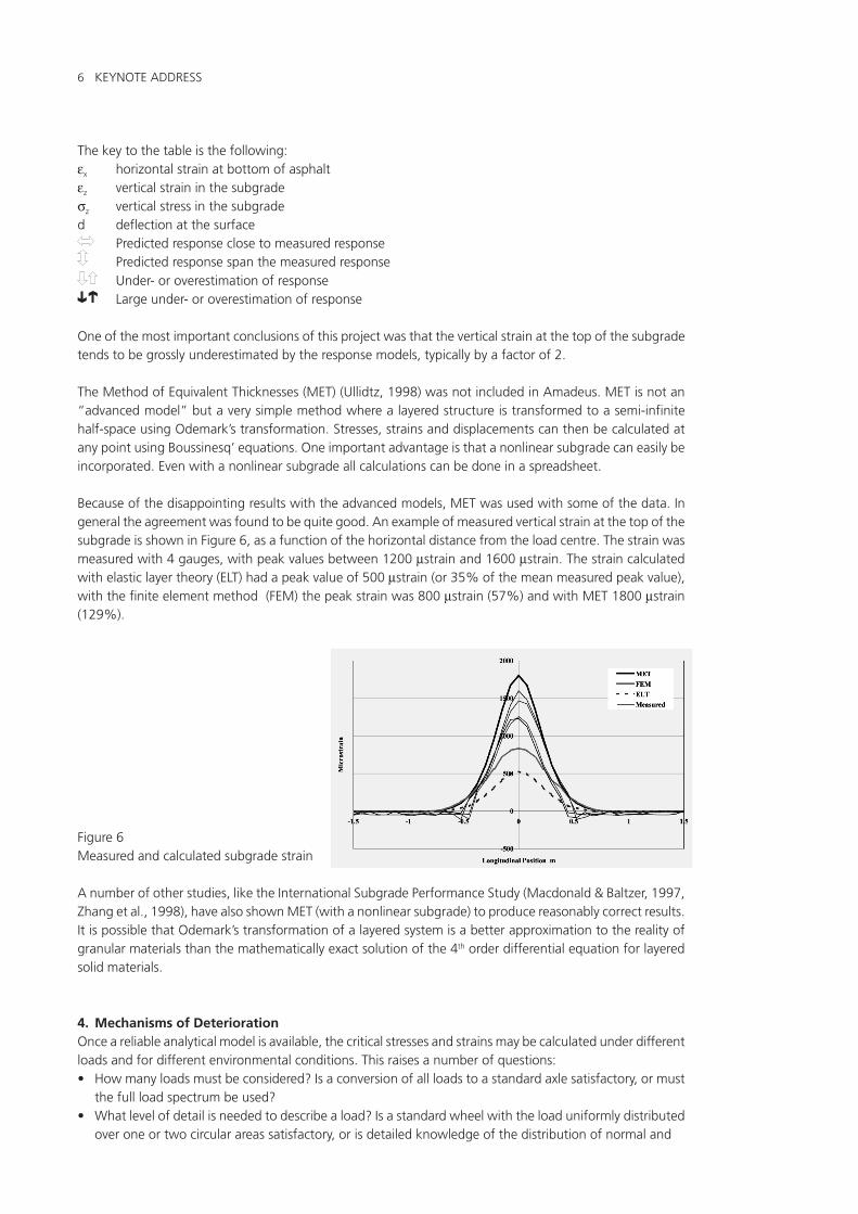
5.6 ResultsThe next three figures show some of the output from a simulation of a pavement section, in terms ofroughness (IRI), permanent deformation and relative asphalt modulus, i.e. the asphalt modulus at any pointin time divided by the mean modulus of intact material. The simulation was repeated 10 times.

Fig. 11. Roughness as a function of time Fig. 12 Permanent deformation as a function of time

Fig. 13Relative asphalt modulus as a function of time

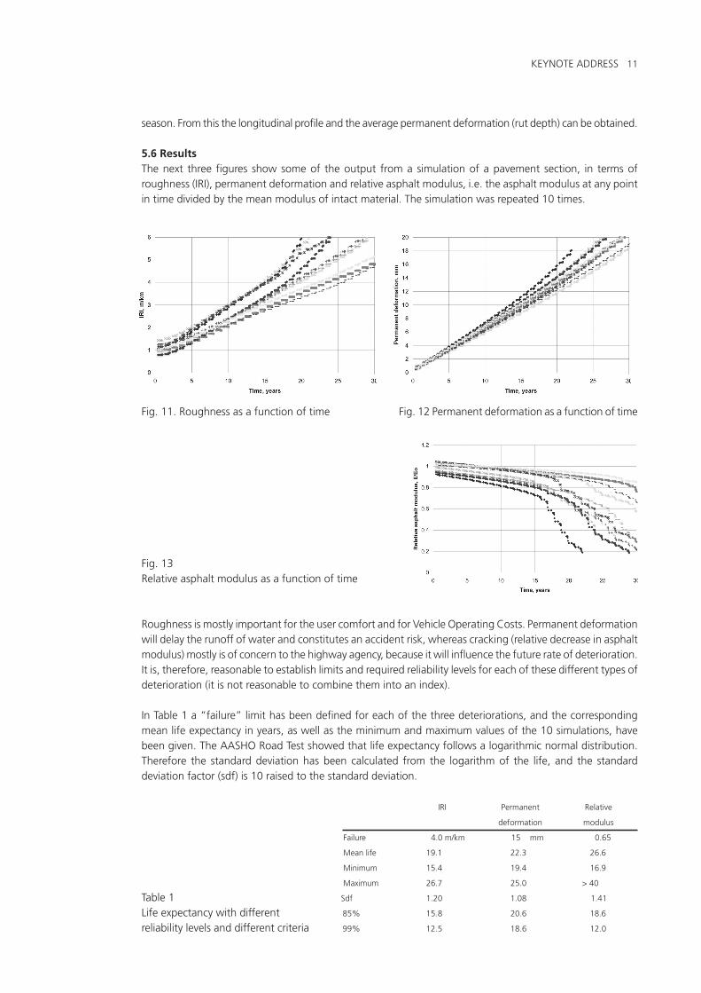
Roughness is mostly important for the user comfort and for Vehicle Operating Costs. Permanent deformationwill delay the runoff of water and constitutes an accident risk, whereas cracking (relative decrease in asphaltmodulus) mostly is of concern to the highway agency, because it will influence the future rate of deterioration.It is, therefore, reasonable to establish limits and required reliability levels for each of these different types ofdeterioration (it is not reasonable to combine them into an index).

In Table 1 a “failure” limit has been defined for each of the three deteriorations, and the correspondingmean life expectancy in years, as well as the minimum and maximum values of the 10 simulations, havebeen given. The AASHO Road Test showed that life expectancy follows a logarithmic normal distribution.Therefore the standard deviation has been calculated from the logarithm of the life, and the standarddeviation factor (sdf) is 10 raised to the standard deviation.

IRI Permanent Relative

deformation modulus

Failure 4.0 m/km 15 mm 0.65

Mean life 19.1 22.3 26.6

Minimum 15.4 19.4 16.9

Maximum 26.7 25.0 > 40

Table 1 Sdf 1.20 1.08 1.41

Life expectancy with different 85% 15.8 20.6 18.6

reliability levels and different criteria 99% 12.5 18.6 12.0

12 KEYNOTE ADDRESS

With a required reliability level of 85% the roughness criterion will result in the shortest life expectancy,whereas the relative modulus is controlling at a level of 99%.

6. Computer Simulation of a Granular MaterialIn simulating the performance of a pavement section, a large number of assumptions were made. One ofthese was that the theories of solid (or continuum) mechanics could be used with pavement materials. Mostpavement materials are not solid, however, but consist of grains, and in granular materials, including asphalt,there is no strain field (except within the individual grains, and this has little influence on the overalldeformation). There are forces (normal and shear) between the grains, and displacements (translation androtation) of the grains.

Another assumption was that the deterioration was a function of some response parameter, tensile strain atthe bottom of the asphalt layer or compressive strain at the top of the unbound layers. These relationshipsare purely phenomenological and do not describe the mechanism of deterioration.

To get a better understanding of granular materials the Distinct Element Method (DEM) (Cundall, 1978) iswell suited. In DEM each grain is free to move. The calculation of forces and displacements is done in shortincrements of time. At the beginning of an increment all the forces on the grains should be known. At thestart of the simulation the forces could be the force of gravity on each grain or externally applied forces.

From the known forces on the elements, the accelerations, velocities and displacements, at the end of thetime step, are calculated. New contacts resulting from the change in geometry are then detected, and finallynew forces are calculated from the movements at the contacts and the contact properties. Contact detectionis time consuming and is usually not done in every time step.

Most models use an explicit integration of the equations of motion (the second central difference method),whereas Dem2D, used in the following (Ullidtz, 1998), makes use of the “Constant Average AccelerationMethod” suggested by Ghaboussi et al. (1993). This is an implicit integration of the equations of motion,where the implicit equations are solved iteratively. This ensures compatibility between accelerations andforces at the end of the time increment.

Fig. 14Sample of grains during compaction

Figure 14 shows a two dimensional (plane strain) sample of “grains” during compaction. In this case aconstant stress of 250 kPa was applied to the sides of the box. Once compaction was completed cohesionand cohesive strength were added to the contact points. Cohesion will increase the permissible shear forceand the cohesive strength will allow tensile forces at the contact points. The tensile stiffness is also input

KEYNOTE ADDRESS 13

Figure 15 shows the same sample, after compaction and addition of cohesion, when the stress in the verticaldirection has been reduced to 54 kPa. The sample is, thus, still under compression, and in a continuum theminor principal stress would be a compressive stress of 54 kPa. However, the thick (red) lines indicate tensileforces between the grains, with a maximum tensile force of 7.7% of the tensile strenght.

Fig. 15Sample in compression, but with tensile forces

Fig. 16Partial failure

Fig. 17Complete failure

14 KEYNOTE ADDRESS

Figures 16 and 17 show the sample at partial and complete failure. The black points indicate broken contacts.In Figure 16 there are 23 broken contacts.

Fig. 18Shear stress and crack developmentas a function of time

Figure 18 shows the number of broken contacts (to the left) and the shear stress (to the right) as a functionof the time of loading. With 23 broken contacts (Figure 16) the maximum shear stress has not yet beenreached.

One of the advantages of the “virtual” tests compared to real tests, is that tests to failure can be repeatedon exactly identical samples. For one sample seven different stress paths were used, as indicated by thethick, black lines in Figure 19.

The stress paths were (for failures from left to right in Figure 19):

1) Pure tension, zx = zy, ∆zx = -1.25 MPa/sec, shear stress t = 02) Uniaxial tension, zx = 0, ∆zy = -1.25 MPa/sec, hydrostatic stress p = t3) Pure shear, zx = -zy, ∆zy = -1.25 MPa/sec, p = 04) Uniaxial tension, zx = 250 kPa, ∆zy = -1.25 MPa/sec, p = 250 kPa - t5) Uniaxial compression, zx = 0, ∆zy = +1.25 MPa/sec, p = t6) Pure shear, zx = 250 kPa – zy, ∆zy = +1.25 MPa/sec, p = 250 kPa7) Uniaxial compression, zx = 250 kPa, ∆zy = +1.25 MPa/sec, p = 250 kPa + t

Fig. 19Different stress paths to failure

The curve fitted to the failure points has the equation:

(2tp/To) a = (ka-1)/(k+1) * (2p/To + (ka+k)/(ka-1))

where tp could be considered as the permissible shear stressTo is the uniaxial tensile strength (To = 97 kPa)k is the ratio of uniaxial compressive strength to uniaxial tensile strength (To),a is a power. a, To and k are determined by minimizing the differences withthe measured values, in this case a = 1.53 and k = 5.29

Shear stress and number of cracks

0

50

100

150

200

250

300

350

0 0.05 0.1 0.15 0.2 0.25 0.3 0.35 0.4

Time, sec

0

50

100

150

200

250

300

350

Crack

(zx-zy)/2

-zd/2

40 per. Mov. Avg. ((zx-zy)/2)

KEYNOTE ADDRESS 15

In order to investigate the influence of repeated loading on permanent deformation and failure, a samplewas loaded with a constant stress and with a repeated stress (compressive), as shown in Figure 20. Thehorizontal (or confining) stress was kept at zero.

Both the constant stress and the repeated stress were increased linearly from zero to 562.5 kPa during thefirst 10 msec, then kept constant at 562.5 kPa for the constant stress loading. For the repeated loading thestress was kept constant for the next 10 msec, decreased to zero during the following 10 msec and thenkept constant at zero for 10 msec. This cycle was then repeated.

Fig. 20Constant and repeated deviator stress

Figure 21 shows the deviator strain and the number of broken contacts as a function of time. The deviatorstrain is shown, in mstrain, at the left ordinate and the number of broken contacts at the right. During thefirst three loading cycles, or 120 msec of constant load, the (maximum) deviator strain is the same forconstant and repeated loading. The repeated loading reveals that about half of the deviator strain is apermanent or plastic strain, and that the permanent strain is increasing slightly with each loading cycle.

After 120 msec there is an increase in the deviator strain under the constant load, at 160 msec four contactsfail and at 235 msec another two contacts fail. For the repeated loading six contacts fail during the sixthloading cycle, at 170 msec. With both types of loading there is, thus, the same number of failures at thebeginning of the test, at approximately the same time, and the resulting increase in (maximum) deviatorstrain is about the same.

Fig. 21Different performance under constantand repeated loading

After the initial failures, however, the sample behaves quite differently under the two different types ofloading. Under constant loading the deviator strain reaches a level of 540 mstrain and remains stable at thislevel, with no more movement of the grains. Under repeated loading the permanent part of the deviatorstrain increases slightly for each loading cycle, whereas the resilient (or reversible) part remains fairly constant.After 25 cycles (about 1 sec) one more failure occurs and after 52 cycles the sample fails completely.

16 KEYNOTE ADDRESS

The Distinct Element Method may also be used with larger samples of particles. Figure 22 shows a 1000´2000mm “box” filled with 3662 particles. The particles have been compacted in two layers to a thickness of 830mm for the lower layer and 100 mm for the upper layer. Particle size distribution and angularities aredifferent for the two layers. In the upper layer cohesion is assumed between the particles, as well as apermissible tensile force (of 20 N at each contact point). The vectors from the centres of the particles showthe displacement during the first 8 msec of loading on a 150 mm plate at the surface of the sample. At thisload all contacts were intact.

The displacement field is quite different from what would have been obtained in an elastic solid. An examplefrom a Finite Element calculation, with the same proportions and the same centre line deflection, is shownin Figure 23.

Fig. 22Displacement field in particulate sample

Fig. 23Displacement field in elastic solid (FEM)

After 27 msec of loading 15 contact points had failed. The position of the failed contact points and thesequence of the first 5 failures are shown in Figure 24.

Fig. 24Location of failed contacts andsequence of failures (first 5 points)

Cracking appears to be neither “bottom up” nor “top down”.

7. ConclusionSince the first International Conference on Structural Design of Asphalt Pavements in Ann Arbor in 1962,the theory of elasticity has been widely used to model pavement structures, and today it forms part of manynational pavement design standards. It is still an open question, however, how well the theory of elasticitypredicts the pavement response under load. Pavement materials are rarely elastic solids, more often they areparticulate, and measurements have repeatedly shown important differences from theoretical values.