Analytical Tools Cheatsheet

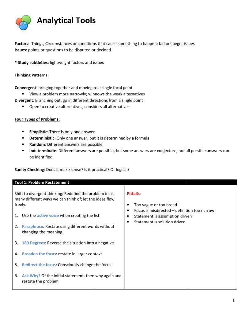
Analytical Tools

Factors: Things, Circumstances or conditions that cause something to happen; factors beget issues

Issues: points or questions to be disputed or decided

* Study subtleties: lightweight factors and issues

Thinking Patterns:

Convergent: bringing together and moving to a single focal point

� View a problem more narrowly; winnows the weak alternatives

Divergent: Branching out, go in different directions from a single point

� Open to creative alternatives, considers all alternatives

Four Types of Problems:

� Simplistic: There is only one answer

� Deterministic: Only one answer, but it is determined by a formula

� Random: Different answers are possible

� Indeterminate: Different answers are possible, but some answers are conjecture, not all

be identified

Sanity Checking: Does it make sense? Is it practical? Or logical?

Tool 1: Problem Restatement

Shift to divergent thinking: Redefine the problem in as

many different ways we can think of; let the ideas flow

freely.

1. Use the active voice when creating the list.

2. Paraphrase: Restate using different wo

changing the meaning

3. 180 Degrees: Reverse the situation into a negative

4. Broaden the focus: restate in larger context

5. Redirect the focus: Consciously change

6. Ask Why? Of the initial statement, then why again and

restate the problem

Analytical Tools

: Things, Circumstances or conditions that cause something to happen; factors beget issues

: points or questions to be disputed or decided

: lightweight factors and issues

: bringing together and moving to a single focal point

View a problem more narrowly; winnows the weak alternatives

: Branching out, go in different directions from a single point

Open to creative alternatives, considers all alternatives

: There is only one answer

: Only one answer, but it is determined by a formula

: Different answers are possible

: Different answers are possible, but some answers are conjecture, not all

: Does it make sense? Is it practical? Or logical?

Shift to divergent thinking: Redefine the problem in as

many different ways we can think of; let the ideas flow

when creating the list.

: Restate using different words without

: Reverse the situation into a negative

: restate in larger context

: Consciously change the focus

Of the initial statement, then why again and

Pitfalls:

• Too vague or too broad

• Focus is misdirected – definition too narrow

• Statement is assumption driven

• Statement is solution driven

1

: Things, Circumstances or conditions that cause something to happen; factors beget issues

: Different answers are possible, but some answers are conjecture, not all possible answers can

definition too narrow

Statement is assumption driven

2

Tool 2: Pros and Cons

Steps for Creating Pros and Cons:

1. List all Pros

2. List all Cons

3. Review and consolidate the Cons, merging and

eliminating

4. Neutralize as many Cons as possible

5. Compare the Pros and unalterable Cons for all options

6. Pick one option

Pro and Cons allows distilling what be the consequence if

one was selected.

It will be easier to do Cons humans are compulsively

critical, but sometime negatives can overwhelm the

positive.

Tool 3: Divergent / Convergent Thinking

Step 1. Brainstorm (Divergent)

Step 2. Winnow and Cluster (Convergent)

Step 3. Select practical, promising ideas (Convergent)

Rules of Divergent Thinking:

• The more ideas, the better

• Build upon one idea to another

• Wacky ideas are acceptable; break conventional

wisdom

• Don’t evaluate the ideas

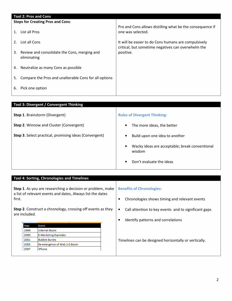
Tool 4: Sorting, Chronologies and Timelines

Step 1. As you are researching a decision or problem, make

a list of relevant events and dates, Always list the dates

first.

Step 2. Construct a chronology, crossing off events as they

are included.

Benefits of Chronologies:

• Chronologies shows timing and relevant events

• Call attention to key events and to significant gaps

• Identify patterns and correlations

Timelines can be designed horizontally or vertically.

3

Tool 5: Casual Flow Diagram

Casual Flow Diagram Construction Steps:

1. Identify major factors

2. Identify Cause-and-Effect Relationships

3. Characterize the relationship (Direct or Inverse)

4. Diagram the relationship

5. Analyze the behavior of the relationship when it is

integrated

CFD benefits:

� Identifies the major factors – the engines – that drive

the system; how they interact, and whether these

interactions are direct or inverse related.

� Enables us to view the cause and effect relationships

as an integrated system and discover linkages that are

formerly dimmed and obscured

� Facilitates our determining the main source of the

problem

� Enables us to conceive alternative corrective

measures and to estimate respective effects.

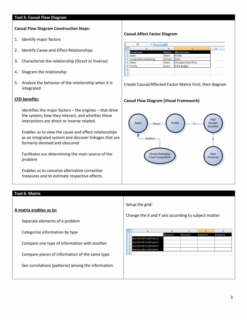
Casual Affect Factor Diagram

Create Causal/Affected Factor Matrix First; then diagram

Casual Flow Diagram (Visual Framework)

Tool 6: Matrix

A matrix enables us to:

� Separate elements of a problem

� Categorize information by type

� Compare one type of information with another

� Compare pieces of information of the same type

� See correlations (patterns) among the information

Setup the grid:

Change the X and Y axis according to subject matter:

4

Tool 7: Decision Event Tree (DET)

Steps to Building a Decision Event Tree:

1. Identify the problem

2. Identify the major factors/issues (the decision &

events) to be addressed in the analysis

3. Identify alternatives for each of these factors/issues

4. Construct the tree portraying all important alternative

scenarios

5. Ensure that the decision/events at each branches of

the tree are mutually exclusive

6. Ensure that the decisions/events at each brach are

collectively exhaustive

Decision Event Tree Offers:

� It dissects a scenario into its sequential events

� It shows clearly the cause and effect linkages,

indicating which decisions and events precede and

follow others

� Shows which decisions and events are dependent on

others

� It shows where the linkages are the strongest &

weakest

� Enables us to visually compare how one scenario

differs from another

� Reveals alternatives we might otherwise not perceive

& enables us to analyze them – separately,

systematically and sufficiently.

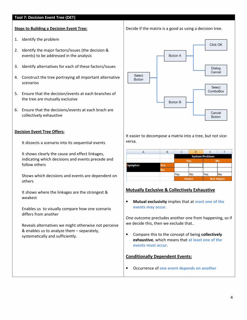
Decide if the matrix is a good as using a decision tree.

It easier to decompose a matrix into a tree, but not vice-

versa.

Mutually Exclusive & Collectively Exhaustive

• Mutual exclusivity implies that at most one of the

events may occur.

One outcome precludes another one from happening, so if

we decide this, then we exclude that..

• Compare this to the concept of being collectively

exhaustive, which means that at least one of the

events must occur.

Conditionally Dependent Events:

• Occurrence of one event depends on another

5

Tool 8: Weighted Ranking

Steps of Weighted Ranking:

1. List all of the major criteria for ranking

2. Pair-rank the criteria

3. Select the top several criteria and weight them in

percentiles (their sum must = 1.0)

4. Construct a Weighted Ranking Matrix and enter

items to be ranked, selected criteria, and the criteria

weights.

5. Pair-rank all the items by each criterion, recording in

the appropriate space the number of votes each

item receives.

6. Multiply the number of votes/tallies/observations by

the respective criterions weight.

7. Add the weighted values for each item and enter the

sums in the column labeled Total votes

8. Determine the final rankings and enter them in the

last column labeled ‘Final Ranking’ – item with the

most points is ranked highest.

9. Perform a sanity check

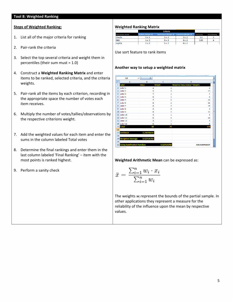
Weighted Ranking Matrix

Use sort feature to rank items

Another way to setup a weighted matrix

Weighted Arithmetic Mean can be expressed as:

The weights wi represent the bounds of the partial sample. In

other applications they represent a measure for the

reliability of the influence upon the mean by respective

values.

6

Tool 9: Hypothesis Testing

Steps:

1. Generate a hypothesis. Eliminate any

implausible hypothesis and combine any

similarities.

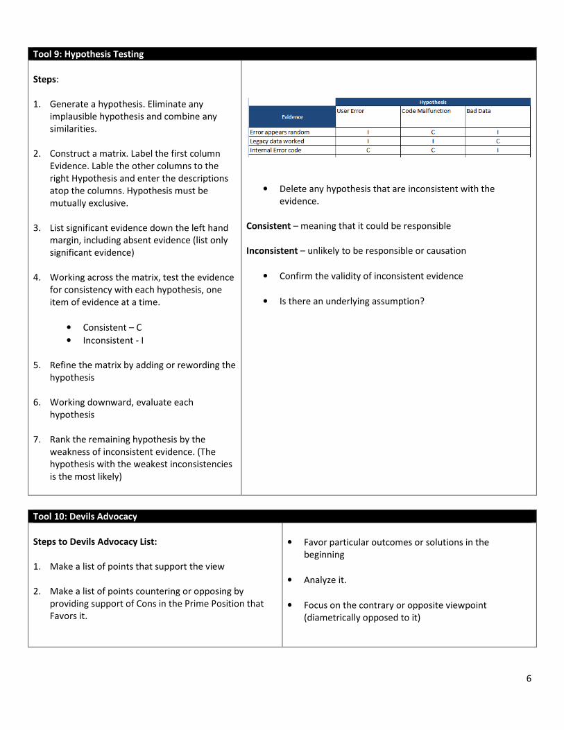
2. Construct a matrix. Label the first column

Evidence. Lable the other columns to the

right Hypothesis and enter the descriptions

atop the columns. Hypothesis must be

mutually exclusive.

3. List significant evidence down the left hand

margin, including absent evidence (list only

significant evidence)

4. Working across the matrix, test the evidence

for consistency with each hypothesis, one

item of evidence at a time.

• Consistent – C

• Inconsistent - I

5. Refine the matrix by adding or rewording the

hypothesis

6. Working downward, evaluate each

hypothesis

7. Rank the remaining hypothesis by the

weakness of inconsistent evidence. (The

hypothesis with the weakest inconsistencies

is the most likely)

• Delete any hypothesis that are inconsistent with the

evidence.

Consistent – meaning that it could be responsible

Inconsistent – unlikely to be responsible or causation

• Confirm the validity of inconsistent evidence

• Is there an underlying assumption?

Tool 10: Devils Advocacy

Steps to Devils Advocacy List:

1. Make a list of points that support the view

2. Make a list of points countering or opposing by

providing support of Cons in the Prime Position that

Favors it.

• Favor particular outcomes or solutions in the

beginning

• Analyze it.

• Focus on the contrary or opposite viewpoint

(diametrically opposed to it)

7

Tool 11a: Probability Tree

Steps for Developing a Probability Tree:

1. Identify the problem

2. Identify the major decisions and events to be analyzed

3. Construct a decision and events to be analyzed.

4. Construct a decision/event tree portraying all

important alternative scenarios

5. Ensure each branch is mutually exclusive and are

collectively exhaustive.

6. Assign a probability to each decision/event. Each

Branch must equal 1.0 *

7. Calculate the conditional probability of each individual

scenario.

8. Calculate the answers to probability questions relating

to the decision/event

* In numerical possibilities, an event cannot occur more

times than its possibility of occurring. Therefore,

probability can NEVER be greater than 1 or 100 percent.

Probability Rules (Add or Multiply)

� OR Type (Add): when the combined probability that

two or more events will occur as a result of a single

decision (“or”) the event. 0.3 + 0.5 = 0.8 (P1 + P2)

� AND Type (Multiply): when the probability two or

more events will occur in succession (the “and”

situation), we multiply their individual probabilities 0.5

x 0.5 = 0.25 (P1 x P2)

(Consider two coin tosses)

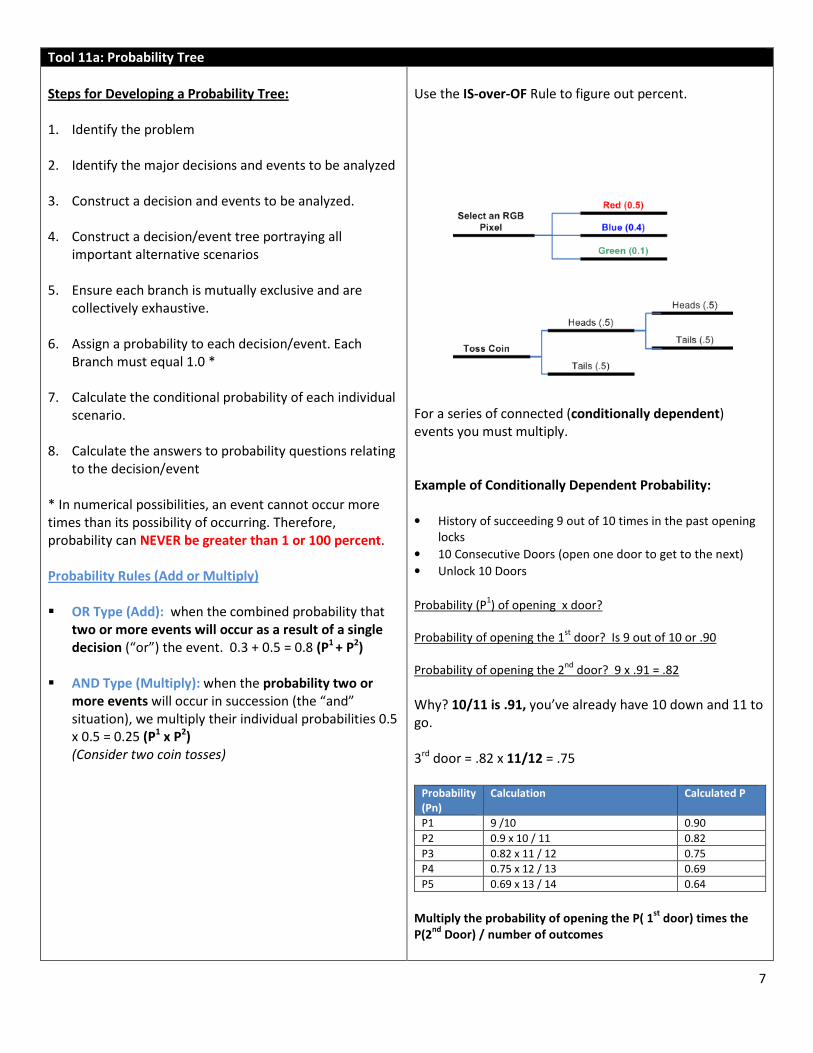
Use the IS-over-OF Rule to figure out percent.

For a series of connected (conditionally dependent)

events you must multiply.

Example of Conditionally Dependent Probability:

• History of succeeding 9 out of 10 times in the past opening

locks

• 10 Consecutive Doors (open one door to get to the next)

• Unlock 10 Doors

Probability (P

1) of opening x door?

Probability of opening the 1st

door? Is 9 out of 10 or .90

Probability of opening the 2nd

door? 9 x .91 = .82

Why? 10/11 is .91, you’ve already have 10 down and 11 to

go.

3rd door = .82 x 11/12 = .75

Probability

(Pn)

Calculation Calculated P

P1 9 /10 0.90

P2 0.9 x 10 / 11 0.82

P3 0.82 x 11 / 12 0.75

P4 0.75 x 12 / 13 0.69

P5 0.69 x 13 / 14 0.64

Multiply the probability of opening the P( 1

st door) times the

P(2nd

Door) / number of outcomes

8

Tool 11b: Probability Refresher

Terms:

� An experiment is a well-defined process with observable outcomes.

� The set or collection of all outcomes of an experiment is called the sample space, S

� An event E is any collection or subset of outcomes from the sample sample.

� An event could have just one outcome and hence it is often called a simple event.

� An event with more than one outcome is called a compound event.

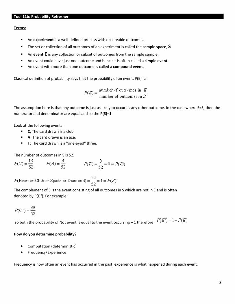
Classical definition of probability says that the probability of an event, P(E) is:

The assumption here is that any outcome is just as likely to occur as any other outcome. In the case where E=S, then the

numerator and denominator are equal and so the P(S)=1.

Look at the following events:

� C: The card drawn is a club.

� A: The card drawn is an ace.

� T: The card drawn is a "one-eyed" three.

The number of outcomes in S is 52.

The complement of E is the event consisting of all outcomes in S which are not in E and is often

denoted by P(E '). For example:

so both the probability of Not event is equal to the event occurring – 1 therefore:

How do you determine probability?

• Computation (deterministic)

• Frequency/Experience

Frequency is how often an event has occurred in the past; experience is what happened during each event.

9

Tool 12: Utility Tree

Steps to Create A Utility Tree:

1. Identify the options and outcomes to be analyzed

2. Identify the perspectives of the analysis

3. Construct a decision/event tree for each option

4. Assign a utility value to each option-outcome

combination – each branch (scenario) of the tree by

asking the Utility Question: If we select this option,

and this outcome occurs, what is the utility from the

perspective of x

5. Assign a probability to each outcome. Determine the

estimate this probability by Asking the Probability

Question: If this option is selected, what the

probability this outcome will occur? (Must add up to

1.0)

6. Determine the expected values by multiplying each

utility by its probability and then adding the expected

value for each option.

7. Determine the ranking of the alternative solutions.


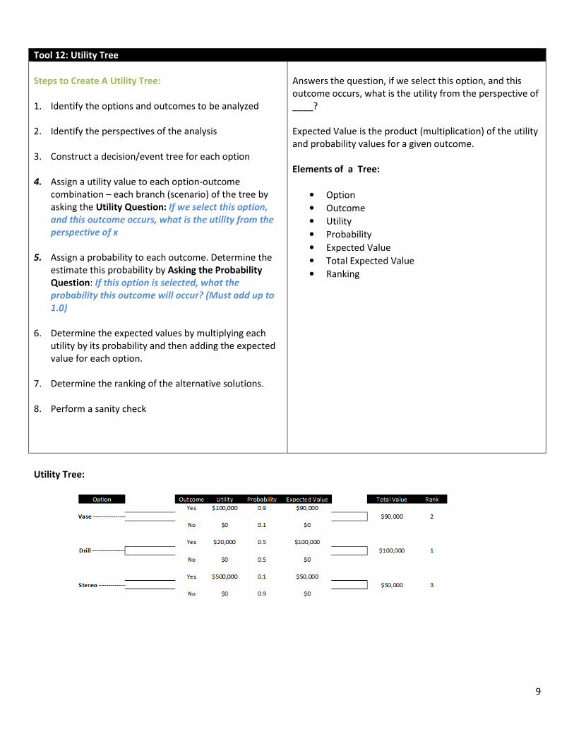
Answers the question, if we select this option, and this

outcome occurs, what is the utility from the perspective of

____?

Expected Value is the product (multiplication) of the utility

and probability values for a given outcome.

Elements of a Tree:

• Option

• Outcome

• Utility

• Probability

• Expected Value

• Total Expected Value

• Ranking

Utility Tree:

10

Tool 13: Utility Matrix

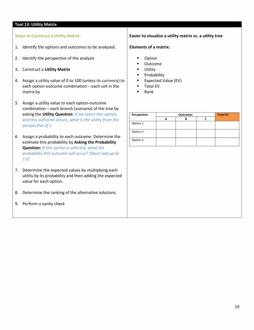
Steps to Construct a Utility Matrix:

1. Identify the options and outcomes to be analyzed.

2. Identify the perspective of the analysis

3. Construct a Utility Matrix

4. Assign a utility value of 0 to 100 (unless its currency) to

each option-outcome combination – each cell in the

matrix by

5. Assign a utility value to each option-outcome

combination – each branch (scenario) of the tree by

asking the Utility Question: If we select this option,

and this outcome occurs, what is the utility from the

perspective of x

6. Assign a probability to each outcome. Determine the

estimate this probability by Asking the Probability

Question: If this option is selected, what the

probability this outcome will occur? (Must add up to

1.0)

7. Determine the expected values by multiplying each

utility by its probability and then adding the expected

value for each option.

8. Determine the ranking of the alternative solutions.


Easier to visualize a utility matrix vs. a utility tree

Elements of a matrix:

� Option

� Outcome

� Utility

� Probability

� Expected Value (EV)

� Total EV

� Rank

Perspective Outcomes Total EV

A B C

Option 1

Option 2

Option 3

11

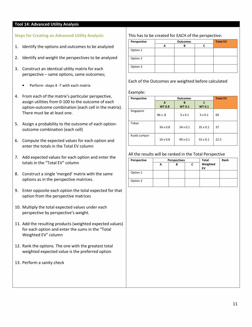
Tool 14: Advanced Utility Analysis

Steps for Creating an Advanced Utility Analysis:

1. Identify the options and outcomes to be analyzed

2. Identify and weight the perspectives to be analyzed

3. Construct an identical utility matrix for each

perspective – same options, same outcomes;

• Perform steps 4 -7 with each matrix

4. From each of the matrix’s particular perspective,

assign utilities from 0-100 to the outcome of each

option-outcome combination (each cell in the matrix).

There must be at least one.

5. Assign a probability to the outcome of each option-

outcome combination (each cell)

6. Compute the expected values for each option and

enter the totals in the Total EV column

7. Add expected values for each option and enter the

totals in the “Total EV” column

8. Construct a single ‘merged’ matrix with the same

options as in the perspective matrices.

9. Enter opposite each option the total expected for that

option from the perspective matrices

10. Multiply the total expected values under each

perspective by perspective’s weight.

11. Add the resulting products (weighted expected values)

for each option and enter the sums in the “Total

Weighted EV” column

12. Rank the options. The one with the greatest total

weighted expected value is the preferred option


This has to be created for EACH of the perspective:

Each of the Outcomes are weighted before calculated

Example:

All the results will be ranked in the Total Perspective


A B C

Option 1

Option 2

Option 3


A

WT 0.8

B

WT 0.1

C

WT 0.1

Singapore

86 x .8

3 x 0.1 3 x 0.1

69

Tokyo

34 x 0.8

34 x 0.1 35 x 0.1

37

Kuala Lumpur

10 x 0.8

90 x 0.1 55 x 0.1

22.5

Perspective Perspectives Total

Weighted

EV

Rank

A B C

Option 1

Option 2

12

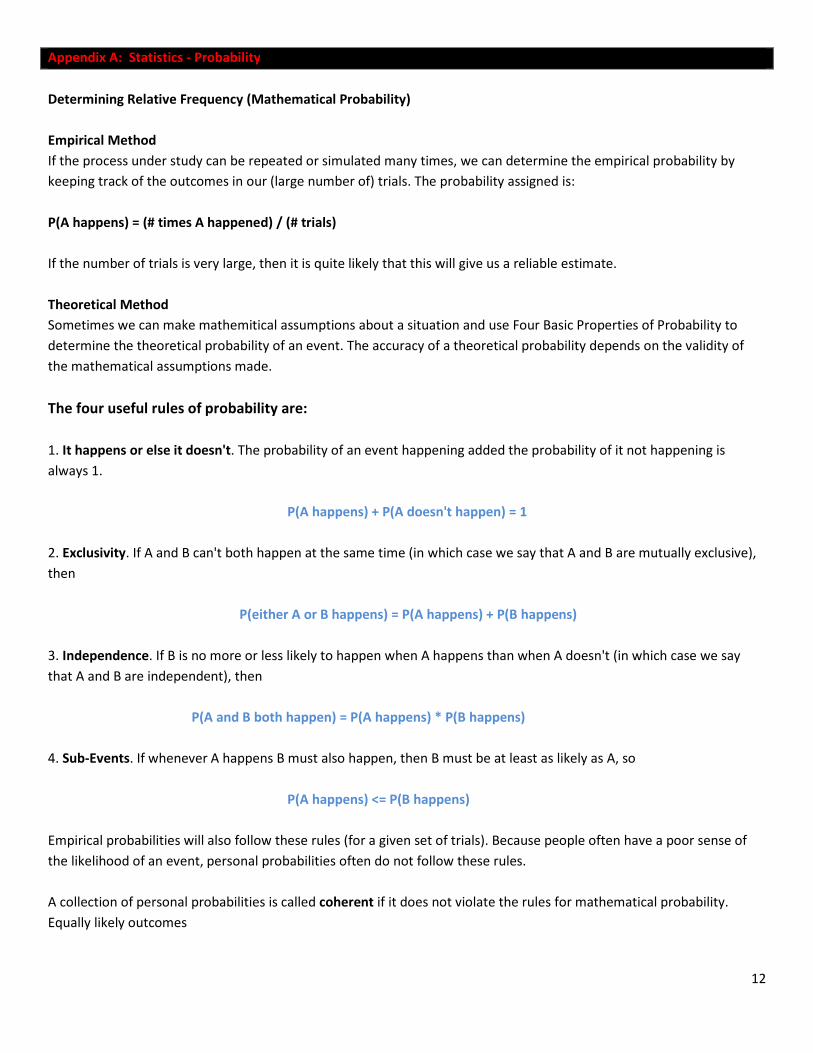
Appendix A: Statistics - Probability

Determining Relative Frequency (Mathematical Probability)

Empirical Method

If the process under study can be repeated or simulated many times, we can determine the empirical probability by

keeping track of the outcomes in our (large number of) trials. The probability assigned is:

P(A happens) = (# times A happened) / (# trials)

If the number of trials is very large, then it is quite likely that this will give us a reliable estimate.

Theoretical Method

Sometimes we can make mathemitical assumptions about a situation and use Four Basic Properties of Probability to

determine the theoretical probability of an event. The accuracy of a theoretical probability depends on the validity of

the mathematical assumptions made.

The four useful rules of probability are:

1. It happens or else it doesn't. The probability of an event happening added the probability of it not happening is

always 1.

P(A happens) + P(A doesn't happen) = 1

2. Exclusivity. If A and B can't both happen at the same time (in which case we say that A and B are mutually exclusive),

then

P(either A or B happens) = P(A happens) + P(B happens)

3. Independence. If B is no more or less likely to happen when A happens than when A doesn't (in which case we say

that A and B are independent), then

P(A and B both happen) = P(A happens) * P(B happens)

4. Sub-Events. If whenever A happens B must also happen, then B must be at least as likely as A, so

P(A happens) <= P(B happens)

Empirical probabilities will also follow these rules (for a given set of trials). Because people often have a poor sense of

the likelihood of an event, personal probabilities often do not follow these rules.

A collection of personal probabilities is called coherent if it does not violate the rules for mathematical probability.

Equally likely outcomes

13

One especially important use of these probability rules is the conclusions that can be drawn if we assume that a number

of events are equally likely. If there are only n such events that are possible in a given situation, and all are equally likely

and pair-wise mutually exclusive (no two can happen at once), then each must have probability 1/n.

More complicated situations can be handled by dividing a situation into a number of equally likely outcomes and

counting how many of them are "of interest" (in the event). The probability then is given by (number of interest)/(total

number.

Example 1:

For example, say you're playing with a deck of cards with a friend. Say he challenges you that if you draw an ace on your

first pick, he will have to buy you lunch the next day. How good are your chances of winning? Well, this is a probability

question. Since there are four aces in 52 cards, your chances of winning are 4/52, or 1/13. So, the probability of you're

picking an ace is 1/13, whereas the probability of you not picking an ace is 12/13. The odds are against you, but it isn't

completely unlikely.

Example 2:

Let's take a more complicated example. Let's say you and your friend are playing with two dice. He gives you the same

challenge, except this time, he challenges you to roll two sixes. The probability of rolling a six on each die is 1/6, but

how about both at the same time? To figure the probability out here, we have to multiply the probability of getting a six

on each die. So, we have 1/6 x 1/6, and our probability for rolling two sixes is 1/36. Your chances are even worse here!

Example 3:

Another interesting thing probability can show you that is somewhat practical is your chances of winning the lottery. If

you play one of those 3-digit lottery tickets where you have to guess the 3-digit number exactly, your probability of

winning is 1/1000. You can figure this out by noting that the probability of you're getting the first number right is 1/10.

The probability of getting all three right is then 1/10 x 1/10 x 1/10. Not too good of a chance!

The 4-digit number is even harder! Can you guess what the probability of winning that lottery might be? And even

more amazing is the tiny probability of winning those multi-million dollar lotteries. That would be a little trickier to

figure out, but it is a slightly different problem. Say there are 70 numbers they pick from. Your chances of getting the

first number right is 1/70. But since one ball has been removed, your chances of getting the second number right is

1/69. If there are six numbers picked, can you figure out what the probability of winning this lottery is? (Remember to

multiply all of the individual probabilities together... 1/70 x 1/69 x ...etc.)

14

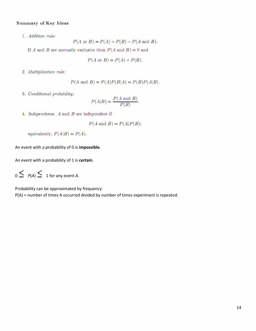
An event with a probability of 0 is impossible.

An event with a probability of 1 is certain.

0 P(A) 1 for any event A.

Probability can be approximated by frequency:

P(A) = number of times A occurred divided by number of times experiment is repeated.

15

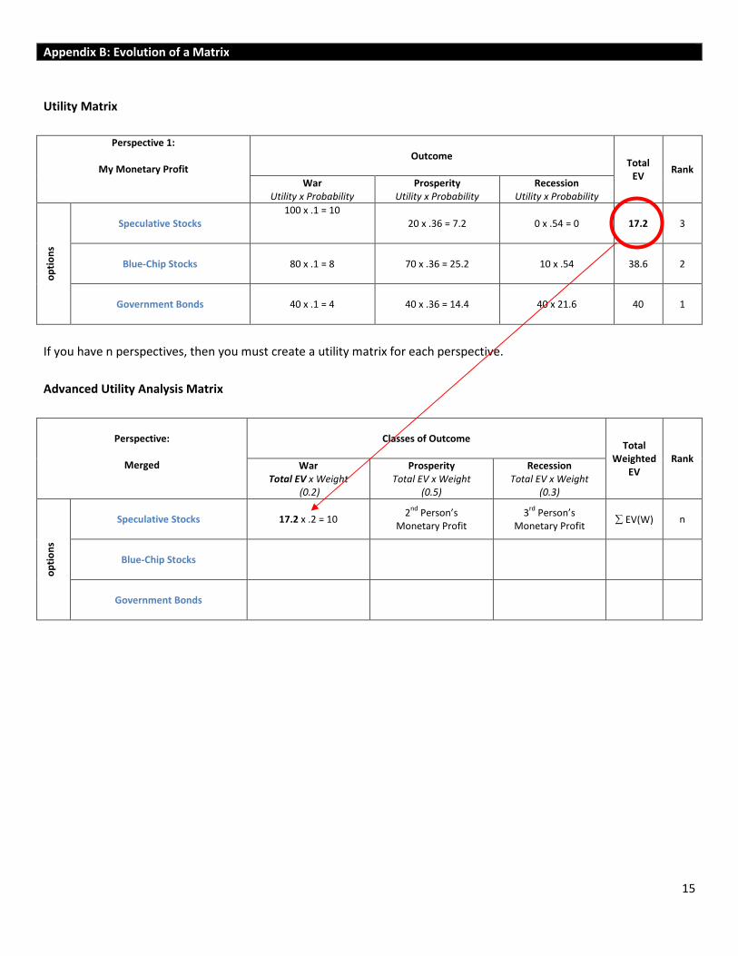
Appendix B: Evolution of a Matrix

Utility Matrix

Perspective 1:

My Monetary Profit

Outcome

Total

EV Rank

War

Utility x Probability

Prosperity


Recession


op

tio

ns

Speculative Stocks

100 x .1 = 10

20 x .36 = 7.2 0 x .54 = 0 17.2 3

Blue-Chip Stocks

80 x .1 = 8 70 x .36 = 25.2 10 x .54 38.6 2

Government Bonds

40 x .1 = 4 40 x .36 = 14.4 40 x 21.6 40 1

If you have n perspectives, then you must create a utility matrix for each perspective.

Advanced Utility Analysis Matrix

Perspective:

Merged

Classes of Outcome

Total

Weighted

EV

Rank War

Total EV x Weight

(0.2)

Prosperity

Total EV x Weight

(0.5)

Recession

Total EV x Weight

(0.3)

op

tio

ns

Speculative Stocks

17.2 x .2 = 10 2

nd Person’s

Monetary Profit

3rd

Person’s

Monetary Profit ∑ EV(W) n

Blue-Chip Stocks

Government Bonds

16

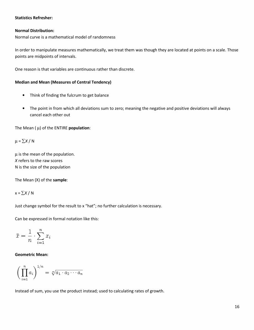
Statistics Refresher:

Normal Distribution:

Normal curve is a mathematical model of randomness

In order to manipulate measures mathematically, we treat them was though they are located at points on a scale. Those

points are midpoints of intervals.

One reason is that variables are continuous rather than discrete.

Median and Mean (Measures of Central Tendency)

• Think of finding the fulcrum to get balance

• The point in from which all deviations sum to zero; meaning the negative and positive deviations will always

cancel each other out

The Mean ( µ) of the ENTIRE population:

µ = ∑X / N

µ is the mean of the population.

X refers to the raw scores

N is the size of the population

The Mean (X) of the sample:

x = ∑X / N

Just change symbol for the result to x “hat”; no further calculation is necessary.

Can be expressed in formal notation like this:

Geometric Mean:

Instead of sum, you use the product instead; used to calculating rates of growth.

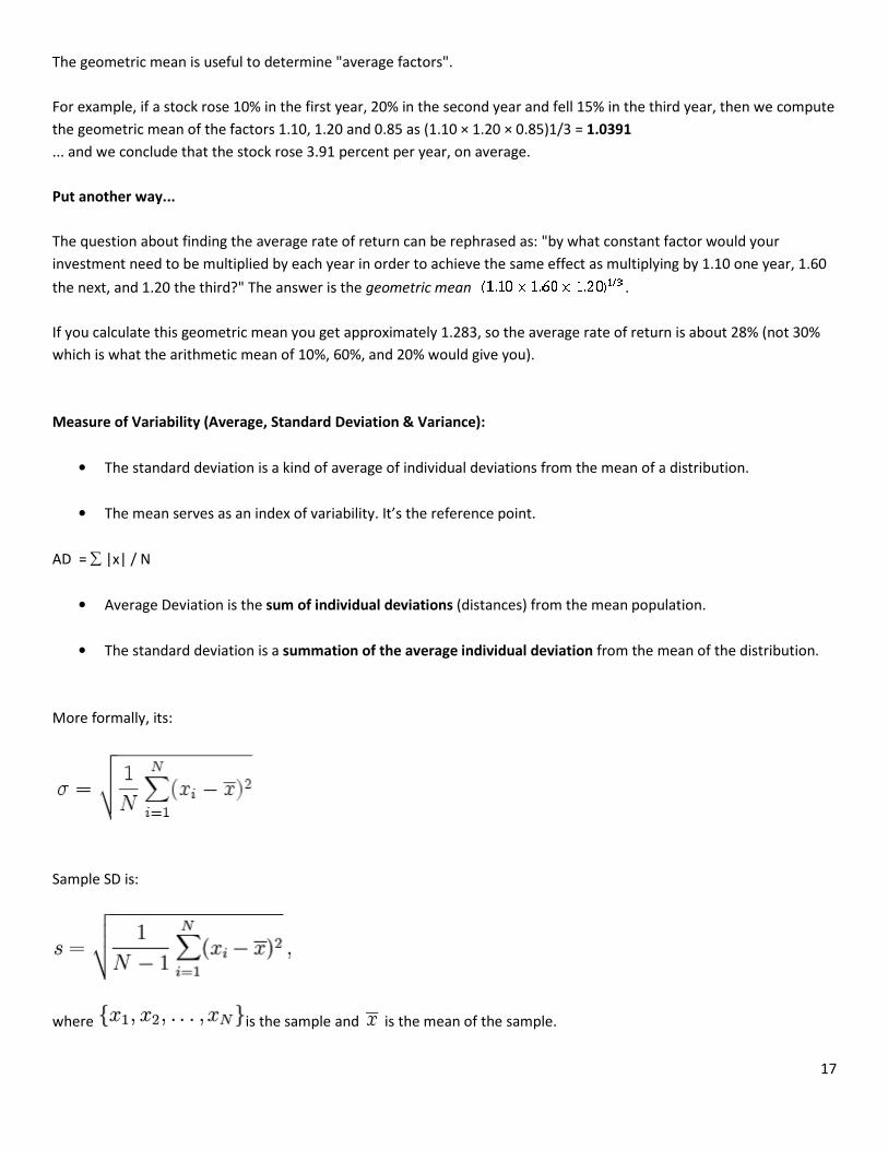
The geometric mean is useful to determine "average factors".

For example, if a stock rose 10% in the first year, 20% in the second year and fell 15% in the third year, then we compute

the geometric mean of the factors 1.10, 1.20 and 0.85 as (1.10 × 1.20

... and we conclude that the stock rose 3.91 percent per year, on average.

Put another way...

The question about finding the average rate of return can be rephrased as: "by what constant factor would your

investment need to be multiplied by each year in order to achieve the same effect as multiplying by 1.10 one year, 1.60

the next, and 1.20 the third?" The answer is the

If you calculate this geometric mean you get approximately 1.283, so the average rate of return

which is what the arithmetic mean of 10%, 60%, and 20% would give you).

Measure of Variability (Average, Standard Deviation & Variance):

• The standard deviation is a kind of average of individual deviations from the mean of a distri

• The mean serves as an index of variability. It’s the reference point.

AD = ∑ |x| / N

• Average Deviation is the sum of individual deviations

• The standard deviation is a summation of the average individual

More formally, its:

Sample SD is:

where is the sample and

The geometric mean is useful to determine "average factors".


the geometric mean of the factors 1.10, 1.20 and 0.85 as (1.10 × 1.20 × 0.85)1/3 = 1.0391

... and we conclude that the stock rose 3.91 percent per year, on average.


ied by each year in order to achieve the same effect as multiplying by 1.10 one year, 1.60

the next, and 1.20 the third?" The answer is the geometric mean .

If you calculate this geometric mean you get approximately 1.283, so the average rate of return

which is what the arithmetic mean of 10%, 60%, and 20% would give you).

(Average, Standard Deviation & Variance):

The standard deviation is a kind of average of individual deviations from the mean of a distri

The mean serves as an index of variability. It’s the reference point.

sum of individual deviations (distances) from the mean population.

summation of the average individual deviation from the mean of the distribution.

is the sample and is the mean of the sample.

17



ied by each year in order to achieve the same effect as multiplying by 1.10 one year, 1.60

If you calculate this geometric mean you get approximately 1.283, so the average rate of return is about 28% (not 30%

The standard deviation is a kind of average of individual deviations from the mean of a distribution.

(distances) from the mean population.

from the mean of the distribution.

18

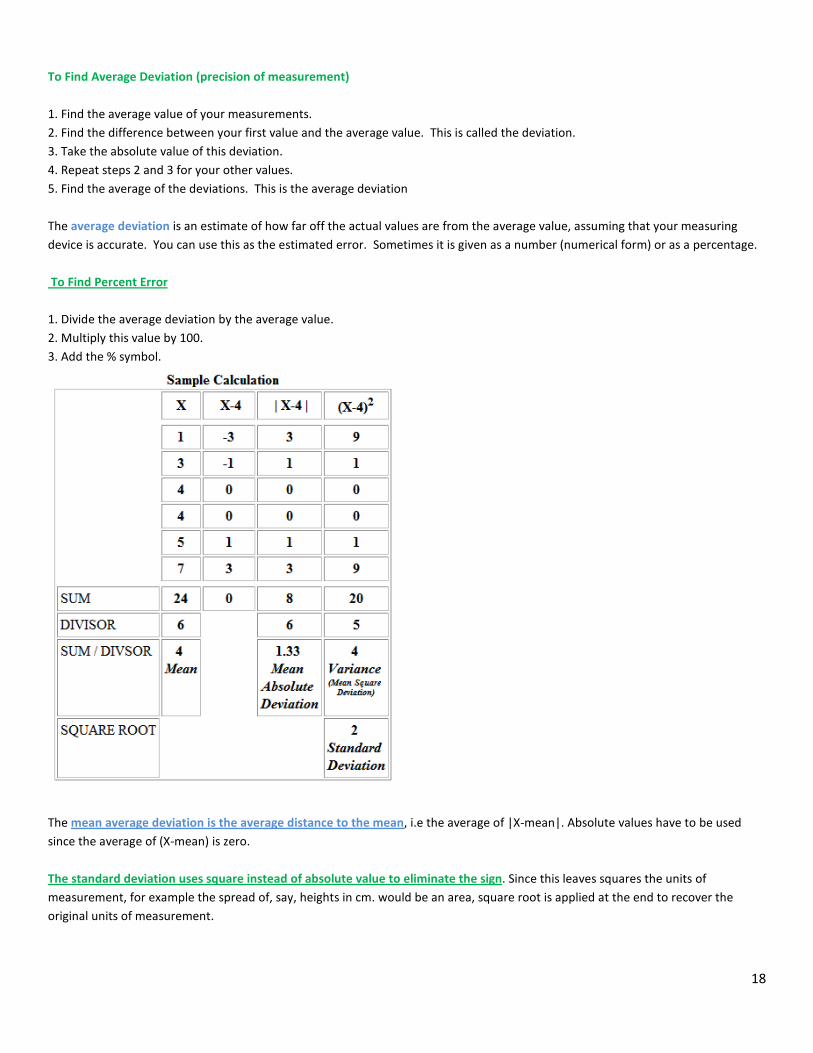
To Find Average Deviation (precision of measurement)

1. Find the average value of your measurements.

2. Find the difference between your first value and the average value. This is called the deviation.

3. Take the absolute value of this deviation.

4. Repeat steps 2 and 3 for your other values.

5. Find the average of the deviations. This is the average deviation

The average deviation is an estimate of how far off the actual values are from the average value, assuming that your measuring

device is accurate. You can use this as the estimated error. Sometimes it is given as a number (numerical form) or as a percentage.

To Find Percent Error

1. Divide the average deviation by the average value.

2. Multiply this value by 100.

3. Add the % symbol.

The mean average deviation is the average distance to the mean, i.e the average of |X-mean|. Absolute values have to be used

since the average of (X-mean) is zero.

The standard deviation uses square instead of absolute value to eliminate the sign. Since this leaves squares the units of

measurement, for example the spread of, say, heights in cm. would be an area, square root is applied at the end to recover the

original units of measurement.

19

The z –score: Standard Score

Makes it possible for individuals (raw scores/votes/values) onto a single, common scale and compare it.

How?

First we need a unit that can be used to compensate for variability in the distribution. To do that, we use a measure of variability.

Divide the raw-score units by the standard deviation, so:

z = x /S

or more formally:

• X is a raw score to be standardized

• σ is the standard deviation of the population

• μ is the mean of the population

...basically you’re dividing each individual deviation by the standard deviation.

20

Correlation: Finding Relationships

• When you want to know the relationships between a set of values (variables)

• Coefficient of correlation is an index of relationship that is high when there is a strong degree of relationship between

variable and low value when the relationship is weak.

• 1.0 is a perfect correlation.

• We have to know not only about the strength, but direction as well. Direct or Indirect (Inverse)

• Note: Any correlation coefficient carries information about two aspects of a relationship: its strength – measured on a scale

from zero to unity – and its direction – indicated by the presence of a minus sign.

Two types of correlation indices:

• Rank-Difference (Spearman)

• Product-Moment (Pearson)

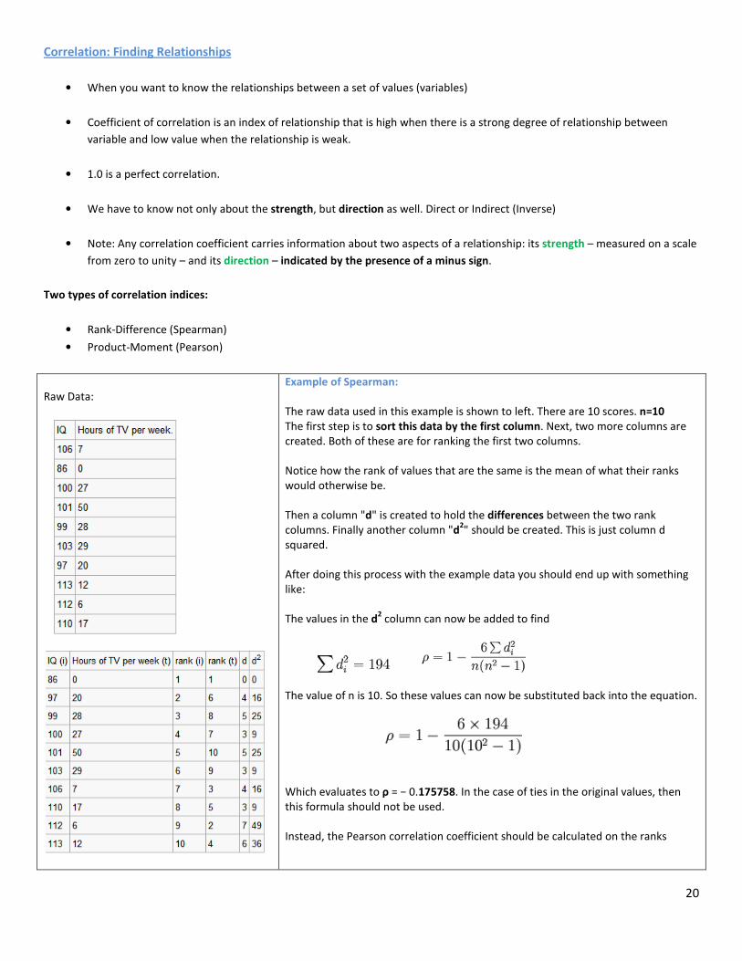
Raw Data:

Example of Spearman:

The raw data used in this example is shown to left. There are 10 scores. n=10

The first step is to sort this data by the first column. Next, two more columns are

created. Both of these are for ranking the first two columns.

Notice how the rank of values that are the same is the mean of what their ranks

would otherwise be.

Then a column "d" is created to hold the differences between the two rank

columns. Finally another column "d2" should be created. This is just column d

squared.

After doing this process with the example data you should end up with something

like:

The values in the d2 column can now be added to find

The value of n is 10. So these values can now be substituted back into the equation.

Which evaluates to ρ = − 0.175758. In the case of ties in the original values, then

this formula should not be used.

Instead, the Pearson correlation coefficient should be calculated on the ranks

21

Regression Analysis:

• Identifying the relationship between a dependent variable and one or more independent variables.

• A model of the relationship is hypothesized, and estimates of the parameter values are used to develop an estimated

regression equation

• .Its purpose is to take a series of independent variables and determine whether a particular dependent variable is related to

the independent variables.

• Regression analysis is very useful in that it does forecasts that do not rely on time. Dependent variables can rely on many

different independent variables.

• A Regression Line displays how well independent and dependent variables fit together. Points are plotted on a graph, and

after regression calculation, a line is drawn that is the "best fit" to the points on the graph.

• The closer the line is to each point, the stronger the relationship is between the independent and dependent variables.

Any future forecast on the dependent variable can be found on the regression line.

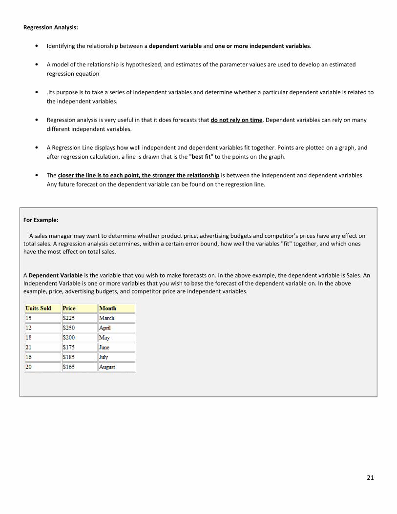
For Example:

A sales manager may want to determine whether product price, advertising budgets and competitor's prices have any effect on

total sales. A regression analysis determines, within a certain error bound, how well the variables "fit" together, and which ones

have the most effect on total sales.

A Dependent Variable is the variable that you wish to make forecasts on. In the above example, the dependent variable is Sales. An

Independent Variable is one or more variables that you wish to base the forecast of the dependent variable on. In the above

example, price, advertising budgets, and competitor price are independent variables.

22

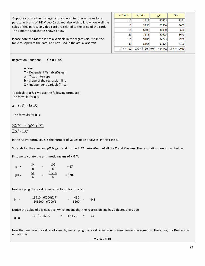
Suppose you are the manager and you wish to forecast sales for a

particular brand of 3-D Video Card. You also wish to know how well the

Sales of this particular video card are related to the price of the card.

The 6 month snapshot is shown below:

Please note the Month is not a variable in the regression, it is in the

table to seperate the data, and not used in the actual analysis.

Regression Equation: Y = a + bX

where:

Y = Dependent Variable(Sales)

a = Y-axis Intercept

b = Slope of the regression line

X = Independent Variable(Price)

To calculate a & b we use the following formulas:

The formula for a is:

a = (µY) - b(µX)

The formula for b is:

ΣXY – n (µX) (µY)

ΣX2 - nX

2

In the Above formulas, n is the number of values to be analyses; in this case 6.

S stands for the sum, and µX & µµµµY stand for the Arithmetic Mean of all the X and Y values. The calculations are shown below.

First we calculate the arithmetic means of X & Y:

µY = SX

n =

102

6 = 17

µX = SY

n =

$1200

6 = $200

Next we plug these values into the formulas for a & b

b = 19910 - 6(200)(17)

245200 - 6(2002)

= -490

5200 = -0.1

Notice the value of b is negative, which means that the regression line has a decreasing slope

a = 17 - (-0.1)200 = 17 + 20 = 37

Now that we have the values of a and b, we can plug these values into our original regression equation. Therefore, our Regression

equation is:

Y = 37 - 0.1X

23

You can now use this equation to forecast sales. For example, you would like to forecast how many video cards you will sell if you

put the card on sale in September for $145. Simply plug this into the equation to find the Y value.

Y = 37 - 0.1(145) = 22.5

Therefore, according to the regression analysis, the forecast for September is between 22 and 23 units sold.

Documents

Analytical Tools Cheatsheet