Embed Size (px)
Citation preview
ASD Technical Guide 3rd Ed. Section 0-1
Section 0
Analytical Spectral Devices, Inc. (ASD)
Technical Guide 3rd Ed. Managing Editor: David C. Hatchell Copyright©1999 Analytical Spectral Devices, Inc. 5335 Sterling Drive Suite A Boulder, CO 80301-2344 USA Phone: 303-444-6522 Fax: 303-444-6825 web: www.asdi.com email: [email protected] 'FieldSpec', 'LabSpec', 'SeaSpec', 'Driftlock' and 'Spectrode' are trademarks of Analytical Spectral Devices, Inc., Boulder, Colorado USA. Other brand and product names are trademarks of their respective holders. The information and specifications contained in this guide are subject to change without notice. Analytical Spectral Devices, Inc. shall not be held liable for technical or editorial omissions or errors made herein; nor for incidental or consequential damages resulting from furnishing, performance or use of this material. This document contains proprietary information protected by copyright. Contact ASD for formal quotations.
ASD Technical Guide 3rd Ed. Section 0-2
Table of Contents Welcome to the ASD Technical Guide...........................................................................................................1-1 Company Profile..........................................................................................................................................1-2 FieldSpec FR ..............................................................................................................................................2-1 FR Post Dispersive Spectrometer .................................................................................................................2-1 FR Direct Path Fiberoptic Input .....................................................................................................................2-1 FR Speed and Sensitivity .............................................................................................................................2-1 FR Longer Fiberoptic Cable Comparison .......................................................................................................2-3 FR Sampling Interval and Spectral Resolution ...............................................................................................3-1 FR Repeatability ..........................................................................................................................................4-1 FR Large Field-of-View ................................................................................................................................4-2 FR Stray Light Rejection ..............................................................................................................................5-1 Stray Light Look Alikes.................................................................................................................................5-7 FR Driftlock .................................................................................................................................................5-7 FR Suggested Set-up...................................................................................................................................6-1 Artificial Illumination and Mineral Reflectance ................................................................................................6-5 FR Foreoptics..............................................................................................................................................7-1 FR Fiberoptic Cable.....................................................................................................................................8-1 FieldSpec FR 1 deg Field-of-View Lens Foreoptic..........................................................................................8-1 FR 1 Deg Field-of-View Mirror Foreoptic........................................................................................................8-2 FR 5 deg Field-of-View Lens Foreoptic..........................................................................................................8-3 FR 8 deg Field-of-View Lens Foreoptic..........................................................................................................8-3 FR 18 deg Field-of-View Tube ......................................................................................................................8-4 FR PistolGrip ...............................................................................................................................................8-5 FieldSpec JR (350 -2500 nm) .......................................................................................................................9-1 JR versus FR Plots ......................................................................................................................................9-1 JR Unique Highlights ...................................................................................................................................9-4 FieldSpec NIR JR (1000 - 2500 nm)..............................................................................................................9-5 FieldSpec UV/VNIR (350 -1050 nm)............................................................................................................10-1 VNIR Post Dispersive Spectrometer............................................................................................................10-1 VNIR Direct Path Fiberoptic Input ...............................................................................................................10-1 VNIR Fiberoptic Cable ...............................................................................................................................10-2 VNIR Speed and Sensitivity........................................................................................................................10-2 VNIR Sampling Interval and Spectral Resolution..........................................................................................10-3 VNIR Ground Truthing Hyperspectral Imagery .............................................................................................10-4 VNIR Stray Light Rejection.........................................................................................................................10-5 VNIR Driftlock............................................................................................................................................10-7 VNIR Large Field-of-View ...........................................................................................................................10-7 VNIR Light Weight, Small, and Wear-able ...................................................................................................10-7 VNIR Upgrade to Dual Spectrometer System ..............................................................................................10-7 VNIR Upgrade to a FieldSpec FR ...............................................................................................................10-7 FieldSpec Dual UV/VNIR (350 -1050 nm) ....................................................................................................10-8 FieldSpec UV/VNIR/CCD ...........................................................................................................................10-8 FieldSpec HandHeld ..................................................................................................................................11-1 HandHeld Post Dispersive Spectrometer .....................................................................................................11-1 HandHeld Speed and Sensitivity.................................................................................................................11-1 HandHeld Sampling Interval and Spectral Resolution ...................................................................................11-2 HandHeld Small Size and Weight ...............................................................................................................11-4 HandHeld Large Field-of-View....................................................................................................................11-4 HandHeld Stray Light Rejection ..................................................................................................................11-5 HandHeld Driftlock.....................................................................................................................................11-8 HandHeld Foreoptics .................................................................................................................................11-9 LabSpec Pro Portable Spectrophotometer...................................................................................................12-1 LabSpec Pro Spectral Ranges ....................................................................................................................12-1 LabSpec Pro Features & Advantages:.........................................................................................................12-1 Fundamentals of Spectroradiometry ............................................................................................................14-1 Illumination Geometry ................................................................................................................................15-1 Wavenumber and Wavelength....................................................................................................................16-1
ASD Technical Guide 3rd Ed. Section 0-3
Spectral Regions .......................................................................................................................................17-1 Reflectance ...............................................................................................................................................18-1 Wavelength and Radiometric Calibration Methods .......................................................................................19-1 Blackbody Radiance and Spectroradiometric Calibration ..............................................................................20-1 The Benifits of Portable NIR Analysis..........................................................................................................21-1 Making an NIR Analyzer Work For You .......................................................................................................22-1 Derivation of Bouguer-Lambert-Beer (BLB) Law ..........................................................................................23-1 Approximating Spot Size............................................................................................................................24-1 Foliar Spectral Features .............................................................................................................................25-1 Vegetation Index Formulas .........................................................................................................................25-2 Water Spectral Features ............................................................................................................................25-3 Glossary ...................................................................................................................................................26-1 Reprints ....................................................................................................................................................27-1 Price List...................................................................................................................................................28-1

ASD Technical Guide 3rd Ed. Section 0-4
ASD Technical Guide 3rd Ed. Section 1-1
Section 1 Welcome to the ASD Technical Guide In this information age we are constantly bombarded by copious quantities of information, both wanted and unwanted, good and bad. Those of us in the business of creating information using the latest in technology are constantly answering requests for information, some simple, others complex and involved. We often end up answering the same questions again and again. In order to increase the efficiency of our work force and provide you with concise information, all wanted and good, we have put together a technical guide to ASD’s spectrophotometer/spectroradiometer product line along with a glossary of terms that are used in the light measurement field. We welcome comments, criticisms and suggestions for the next issue, and we hope that our products will fill your application needs. The management and employees of ASD take pride in our customer service reputation. Our aim is to make sure that each customer understands how our instruments work and how to derive the most information from the data acquired. Please contact us by phone, fax, or email: Phone: 303-444-6522 Fax: 303-444-6825 email: [email protected] web: www.asdi.com
ASD Technical Guide 3rd Ed. Section 1-2
Company Profile Analytical Spectral Devices, Inc. (ASD) was founded in February, 1990. ASD manufactures and sells the FieldSpec, LabSpec, and SeaSpec lines of optical spectrometers (all trademarked by ASD). ASD's facilities occupy 11,000 square feet and include laboratories and equipment for the development, testing, calibration and manufacturing of high spectral resolution spectroradiometers, spectrophotometers, and associated run-time and data analysis software. This equipment includes: analog and digital oscilloscopes, function generators, power supplies, digital logic analyzers, optical benches and fixtures, fiber optic illuminators, monochromators, baffled tanks with optical windows for underwater calibrations, spectral line sources, and NIST traceable calibrated irradiance and radiance sources, computers, CAD software, and embedded software development tools. ASD currently employees a variety of Ph.D. Scientists, Engineers, Bachelors Degreed technicians.
ASD Technical Guide 3rd Ed. Section 2-1
Section 2 FieldSpec FR Several important features of the FieldSpec FR make it the best and unique choice for a field portable spectroradiometer: The FieldSpec FR is a post dispersive spectrometer. The FieldSpec FR spectroradiometer uses a direct path fiber optic input. The FieldSpec FR spectroradiometer has an unbeatable combination of speed and sensitivity. The FieldSpec FR spectroradiometer has the spectral resolution and sampling interval required for ground truthing hyperspectral imagery. The FieldSpec FR spectroradiometer has excellent repeatability. The FieldSpec FR has the largest standard field-of-view of any portable spectroradiometer. The FieldSpec FR spectroradiometer has excellent stray light rejection. The FieldSpec FR spectroradiometer features the unique Driftlock™ dark-drift correction system. FR Post Dispersive Spectrometer All ASD spectrometers are “post-dispersive”. Because portable spectrometers are typically used outside the controlled laboratory environment, they are exposed to much higher levels of ambient light. In almost all cases, some of this ambient light will stray into the sample being measured. The errors produced by this ambient stray light are much greater for a pre-dispersive spectrometer than they are for a spectrometer that is post-dispersive. In a pre-dispersive spectrometer, the sample is illuminated with monochromatic light. Light scattered off or transmitted through the sample is then collected and delivered to the instrument’s detector. Ambient light that strays into the sample being measured is also collected. Thus, both the monochromatic illumination from the instrument and all wavelengths of the ambient stray light are delivered to the detector. Because the stray ambient light signal can represent a large fraction of the total light signal measured by the detector, it is a major source of error. While this source or error can be minimized by completely shielding the sample form all sources of ambient illumination, this often precludes the use of most reflectance and transmittance fiber optic probes. In a post-dispersive spectrometer, the sample is illuminated with white light. Light scattered off or transmitted through the sample is then dispersed and delivered to the entrance slit of the instrument’s spectrometer. As with the pre-dispersive spectrometer, ambient light that strays into the sample being measured is also collected. The difference is that in the post-dispersive instrument, only ambient stray light of the same wavelength as that being measured by the detector is added to the signal resulting from the instrument’s illumination of the sample. Thus, the stray ambient light signal represents a small fraction of the total light signal measured by the detector. FR Direct Path Fiberoptic Input The FieldSpec FR spectroradiometer uses a 1 meter fiber optic input that feeds directly into the spectrometer. There are two advantages to this arrangement. First, the fiber optic input allows the user to quickly move and aim the very lightweight fiber optic probe from point to point without having to move the entire spectroradiometer. Secondly, since the fiber optic is connected directly into the spectroradiometer there is none of the signal losses otherwise associated with detachable couplings (detachable couplings typically result in as high as 50% signal loss). FR Speed and Sensitivity The FieldSpec FR spectroradiometer can record a complete 350 - 2500 nm spectrum in 0.1 seconds. This amazing speed allows the convenience of collecting more data in less time, as well as minimizing errors associated with clouds and wind under solar illumination. Another thing to consider is the number of scans that can be collected in a specified time period. The FieldSpec FR also the only portable spectroradiometer designed with a unique type of high speed bi-directional parallel interface to the controlling computer to allow the averaging of continuous sequences of spectra. A serial interface
ASD Technical Guide 3rd Ed. Section 2-2
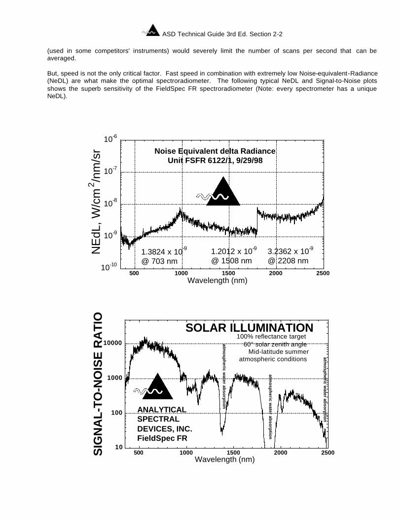
(used in some competitors' instruments) would severely limit the number of scans per second that can be averaged. But, speed is not the only critical factor. Fast speed in combination with extremely low Noise-equivalent-Radiance (NeDL) are what make the optimal spectroradiometer. The following typical NeDL and Signal-to-Noise plots shows the superb sensitivity of the FieldSpec FR spectroradiometer (Note: every spectrometer has a unique NeDL).
10-10
10-9
10-8
10-7
10-6
500 1000 1500 2000 2500
Noise Equivalent delta RadianceUnit FSFR 6122/1, 9/29/98
NE
dL, W
/cm
2 /nm
/sr
Wavelength (nm)
1.3824 x 10⁻⁹ @ 703 nm
1.2012 x 10⁻⁹ @ 1508 nm
3.2362 x 10⁻⁹ @ 2208 nm
500 1000 1500 2000 250010
100
1000
10000
Wavelength (nm)
SIG
NA
L-TO
-NO
ISE
RA
TIO
SOLAR ILLUMINATION
ANALYTICAL SPECTRAL DEVICES, INC.FieldSpec FR
atmo
sph
eric water ab
sorp
tion
atmo
sph
eric water ab
sorp
tion
atmo
sph
eric water ab
sorp
tion
100% reflectance target60° solar zenith angle
Mid-latitude summeratmospheric conditions
ASD Technical Guide 3rd Ed. Section 2-3
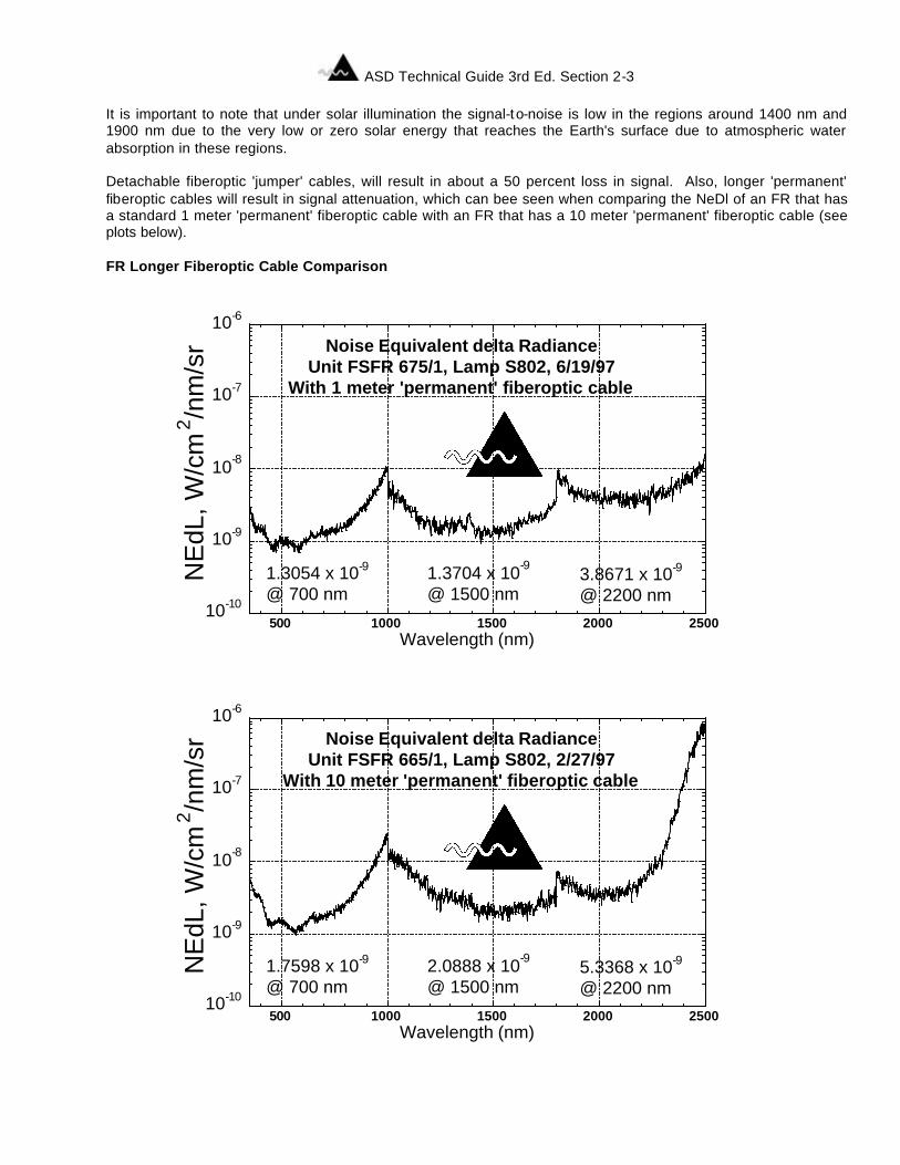
It is important to note that under solar illumination the signal-to-noise is low in the regions around 1400 nm and 1900 nm due to the very low or zero solar energy that reaches the Earth's surface due to atmospheric water absorption in these regions. Detachable fiberoptic 'jumper' cables, will result in about a 50 percent loss in signal. Also, longer 'permanent' fiberoptic cables will result in signal attenuation, which can bee seen when comparing the NeDl of an FR that has a standard 1 meter 'permanent' fiberoptic cable with an FR that has a 10 meter 'permanent' fiberoptic cable (see plots below). FR Longer Fiberoptic Cable Comparison
10-10
10-9
10-8
10-7
10-6
500 1000 1500 2000 2500
Noise Equivalent delta RadianceUnit FSFR 675/1, Lamp S802, 6/19/97
With 1 meter 'permanent' fiberoptic cable
NE
dL, W
/cm
2 /nm
/sr
Wavelength (nm)
1.3054 x 10⁻⁹ @ 700 nm
1.3704 x 10⁻⁹ @ 1500 nm
3.8671 x 10⁻⁹ @ 2200 nm
10-10
10-9
10-8
10-7
10-6
500 1000 1500 2000 2500
Noise Equivalent delta RadianceUnit FSFR 665/1, Lamp S802, 2/27/97
With 10 meter 'permanent' fiberoptic cable
NE
dL, W
/cm
2 /nm
/sr
Wavelength (nm)
1.7598 x 10⁻⁹ @ 700 nm
2.0888 x 10⁻⁹ @ 1500 nm
5.3368 x 10⁻⁹ @ 2200 nm

ASD Technical Guide 3rd Ed. Section 2-4
ASD Technical Guide 3rd Ed. Section 3-1
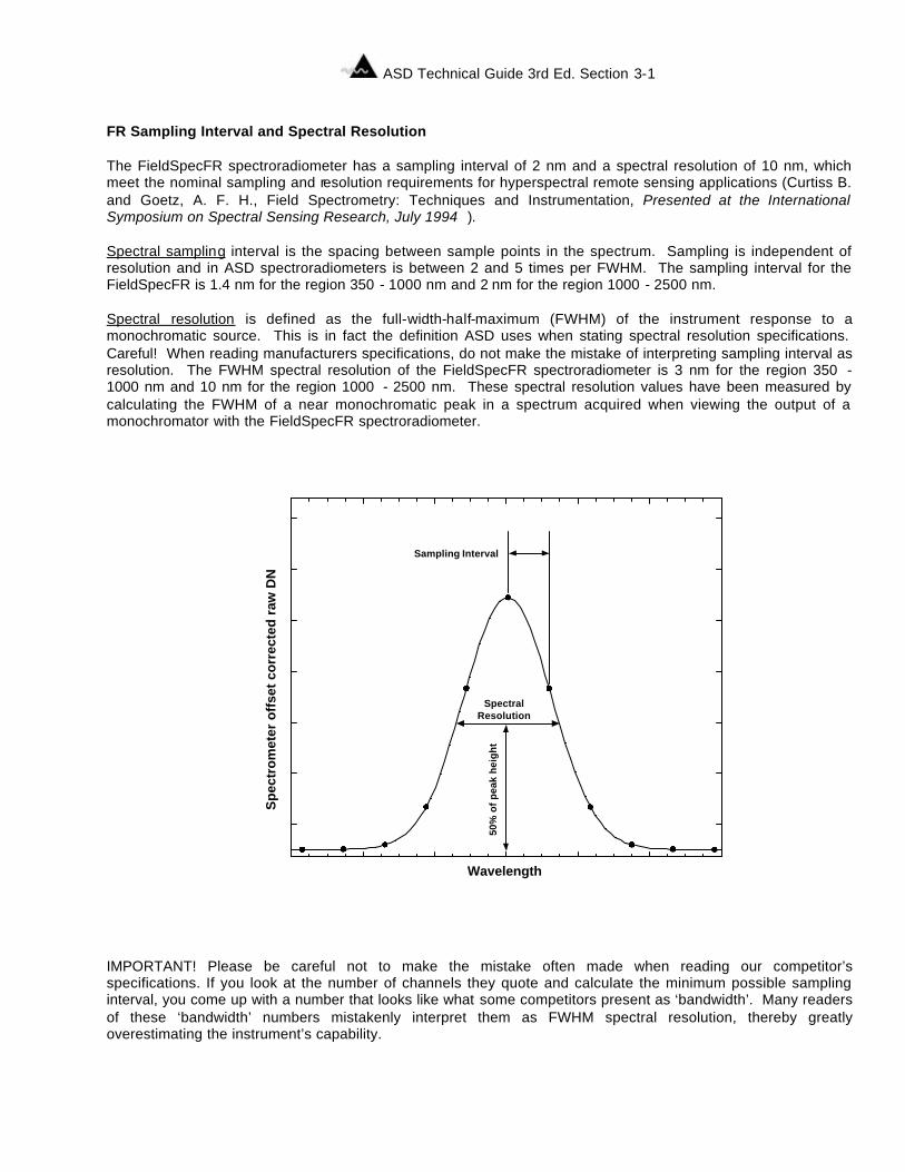
Section 3 FR Sampling Interval and Spectral Resolution The FieldSpecFR spectroradiometer has a sampling interval of 2 nm and a spectral resolution of 10 nm, which meet the nominal sampling and resolution requirements for hyperspectral remote sensing applications (Curtiss B. and Goetz, A. F. H., Field Spectrometry: Techniques and Instrumentation, Presented at the International Symposium on Spectral Sensing Research, July 1994 ). Spectral sampling interval is the spacing between sample points in the spectrum. Sampling is independent of resolution and in ASD spectroradiometers is between 2 and 5 times per FWHM. The sampling interval for the FieldSpecFR is 1.4 nm for the region 350 - 1000 nm and 2 nm for the region 1000 - 2500 nm. Spectral resolution is defined as the full-width-half-maximum (FWHM) of the instrument response to a monochromatic source. This is in fact the definition ASD uses when stating spectral resolution specifications. Careful! When reading manufacturers specifications, do not make the mistake of interpreting sampling interval as resolution. The FWHM spectral resolution of the FieldSpecFR spectroradiometer is 3 nm for the region 350 - 1000 nm and 10 nm for the region 1000 - 2500 nm. These spectral resolution values have been measured by calculating the FWHM of a near monochromatic peak in a spectrum acquired when viewing the output of a monochromator with the FieldSpecFR spectroradiometer. IMPORTANT! Please be careful not to make the mistake often made when reading our competitor’s specifications. If you look at the number of channels they quote and calculate the minimum possible sampling interval, you come up with a number that looks like what some competitors present as ‘bandwidth’. Many readers of these ‘bandwidth’ numbers mistakenly interpret them as FWHM spectral resolution, thereby greatly overestimating the instrument’s capability.
Wavelength
Sampling Interval
SpectralResolution
50%
of
pea
k h
eig
ht
Spe
ctro
met
er o
ffse
t co
rrec
ted
raw
DN
ASD Technical Guide 3rd Ed. Section 3-2
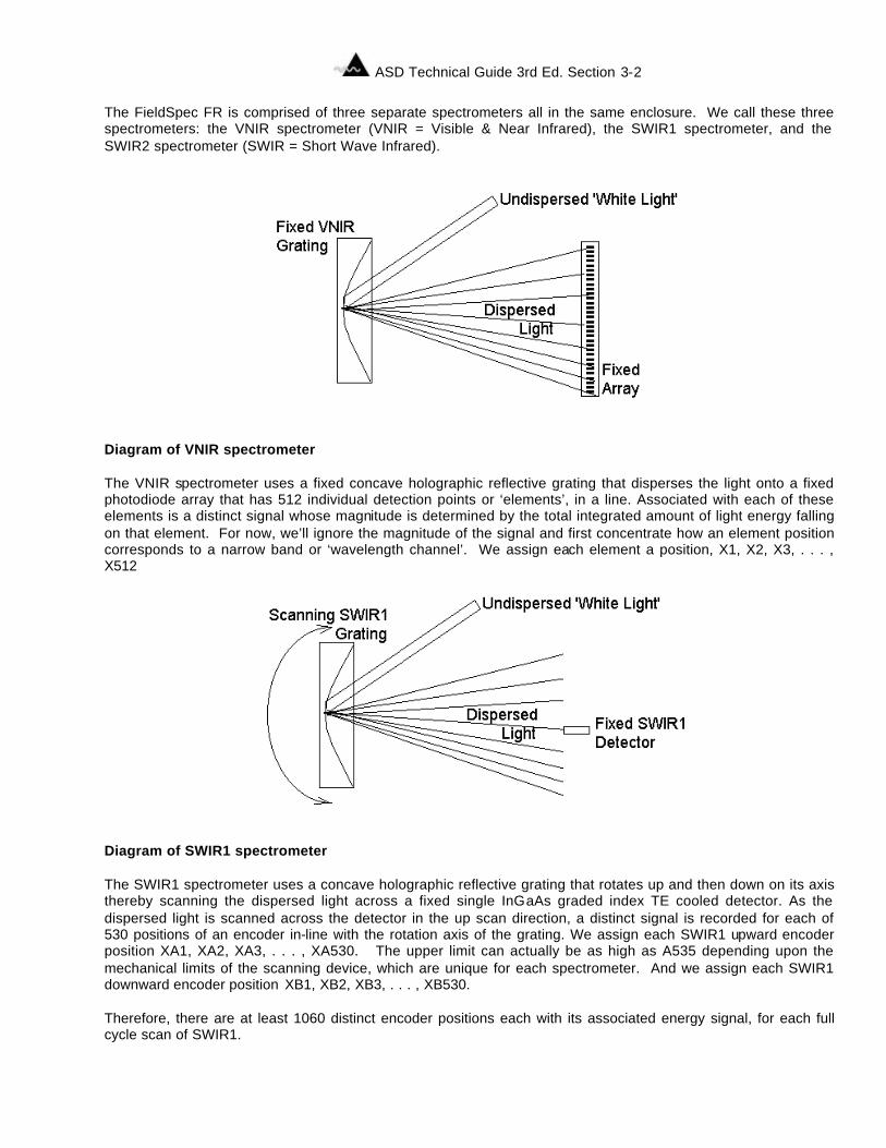
The FieldSpec FR is comprised of three separate spectrometers all in the same enclosure. We call these three spectrometers: the VNIR spectrometer (VNIR = Visible & Near Infrared), the SWIR1 spectrometer, and the SWIR2 spectrometer (SWIR = Short Wave Infrared).
Diagram of VNIR spectrometer The VNIR spectrometer uses a fixed concave holographic reflective grating that disperses the light onto a fixed photodiode array that has 512 individual detection points or ‘elements’, in a line. Associated with each of these elements is a distinct signal whose magnitude is determined by the total integrated amount of light energy falling on that element. For now, we’ll ignore the magnitude of the signal and first concentrate how an element position corresponds to a narrow band or ‘wavelength channel’. We assign each element a position, X1, X2, X3, . . . , X512
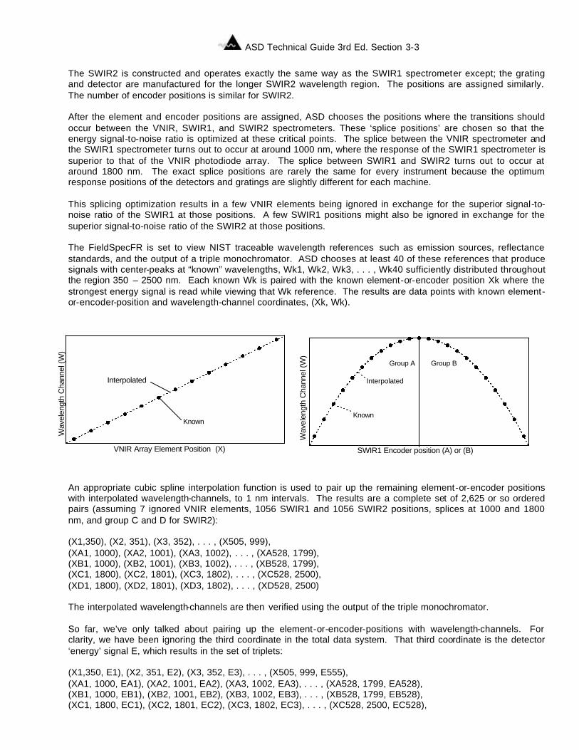
Diagram of SWIR1 spectrometer The SWIR1 spectrometer uses a concave holographic reflective grating that rotates up and then down on its axis thereby scanning the dispersed light across a fixed single InGaAs graded index TE cooled detector. As the dispersed light is scanned across the detector in the up scan direction, a distinct signal is recorded for each of 530 positions of an encoder in-line with the rotation axis of the grating. We assign each SWIR1 upward encoder position XA1, XA2, XA3, . . . , XA530. The upper limit can actually be as high as A535 depending upon the mechanical limits of the scanning device, which are unique for each spectrometer. And we assign each SWIR1 downward encoder position XB1, XB2, XB3, . . . , XB530. Therefore, there are at least 1060 distinct encoder positions each with its associated energy signal, for each full cycle scan of SWIR1.
ASD Technical Guide 3rd Ed. Section 3-3
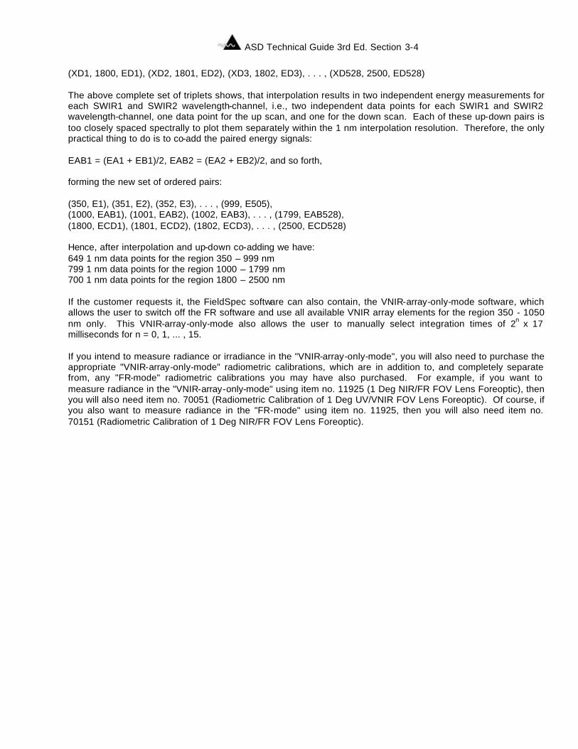
The SWIR2 is constructed and operates exactly the same way as the SWIR1 spectrometer except; the grating and detector are manufactured for the longer SWIR2 wavelength region. The positions are assigned similarly. The number of encoder positions is similar for SWIR2. After the element and encoder positions are assigned, ASD chooses the positions where the transitions should occur between the VNIR, SWIR1, and SWIR2 spectrometers. These ‘splice positions’ are chosen so that the energy signal-to-noise ratio is optimized at these critical points. The splice between the VNIR spectrometer and the SWIR1 spectrometer turns out to occur at around 1000 nm, where the response of the SWIR1 spectrometer is superior to that of the VNIR photodiode array. The splice between SWIR1 and SWIR2 turns out to occur at around 1800 nm. The exact splice positions are rarely the same for every instrument because the optimum response positions of the detectors and gratings are slightly different for each machine. This splicing optimization results in a few VNIR elements being ignored in exchange for the superior signal-to-noise ratio of the SWIR1 at those positions. A few SWIR1 positions might also be ignored in exchange for the superior signal-to-noise ratio of the SWIR2 at those positions. The FieldSpecFR is set to view NIST traceable wavelength references such as emission sources, reflectance standards, and the output of a triple monochromator. ASD chooses at least 40 of these references that produce signals with center-peaks at “known” wavelengths, Wk1, Wk2, Wk3, . . . , Wk40 sufficiently distributed throughout the region 350 – 2500 nm. Each known Wk is paired with the known element-or-encoder position Xk where the strongest energy signal is read while viewing that Wk reference. The results are data points with known element-or-encoder-position and wavelength-channel coordinates, (Xk, Wk). An appropriate cubic spline interpolation function is used to pair up the remaining element-or-encoder positions with interpolated wavelength-channels, to 1 nm intervals. The results are a complete set of 2,625 or so ordered pairs (assuming 7 ignored VNIR elements, 1056 SWIR1 and 1056 SWIR2 positions, splices at 1000 and 1800 nm, and group C and D for SWIR2): (X1,350), (X2, 351), (X3, 352), . . . , (X505, 999), (XA1, 1000), (XA2, 1001), (XA3, 1002), . . . , (XA528, 1799), (XB1, 1000), (XB2, 1001), (XB3, 1002), . . . , (XB528, 1799), (XC1, 1800), (XC2, 1801), (XC3, 1802), . . . , (XC528, 2500), (XD1, 1800), (XD2, 1801), (XD3, 1802), . . . , (XD528, 2500) The interpolated wavelength-channels are then verified using the output of the triple monochromator. So far, we’ve only talked about pairing up the element-or-encoder-positions with wavelength-channels. For clarity, we have been ignoring the third coordinate in the total data system. That third coordinate is the detector ‘energy’ signal E, which results in the set of triplets: (X1,350, E1), (X2, 351, E2), (X3, 352, E3), . . . , (X505, 999, E555), (XA1, 1000, EA1), (XA2, 1001, EA2), (XA3, 1002, EA3), . . . , (XA528, 1799, EA528), (XB1, 1000, EB1), (XB2, 1001, EB2), (XB3, 1002, EB3), . . . , (XB528, 1799, EB528), (XC1, 1800, EC1), (XC2, 1801, EC2), (XC3, 1802, EC3), . . . , (XC528, 2500, EC528),
Wav
elen
gth
Cha
nnel
(W)
VNIR Array Element Position (X)
Interpolated
Known
Wav
elen
gth
Cha
nnel
(W)
SWIR1 Encoder position (A) or (B)
Group A Group B
Known
Interpolated
ASD Technical Guide 3rd Ed. Section 3-4
(XD1, 1800, ED1), (XD2, 1801, ED2), (XD3, 1802, ED3), . . . , (XD528, 2500, ED528) The above complete set of triplets shows, that interpolation results in two independent energy measurements for each SWIR1 and SWIR2 wavelength-channel, i.e., two independent data points for each SWIR1 and SWIR2 wavelength-channel, one data point for the up scan, and one for the down scan. Each of these up-down pairs is too closely spaced spectrally to plot them separately within the 1 nm interpolation resolution. Therefore, the only practical thing to do is to co-add the paired energy signals: EAB1 = (EA1 + EB1)/2, EAB2 = (EA2 + EB2)/2, and so forth, forming the new set of ordered pairs: (350, E1), (351, E2), (352, E3), . . . , (999, E505), (1000, EAB1), (1001, EAB2), (1002, EAB3), . . . , (1799, EAB528), (1800, ECD1), (1801, ECD2), (1802, ECD3), . . . , (2500, ECD528) Hence, after interpolation and up-down co-adding we have: 649 1 nm data points for the region 350 – 999 nm 799 1 nm data points for the region 1000 – 1799 nm 700 1 nm data points for the region 1800 – 2500 nm If the customer requests it, the FieldSpec software can also contain, the VNIR-array-only-mode software, which allows the user to switch off the FR software and use all available VNIR array elements for the region 350 - 1050 nm only. This VNIR-array-only-mode also allows the user to manually select integration times of 2n x 17 milliseconds for n = 0, 1, ... , 15. If you intend to measure radiance or irradiance in the "VNIR-array-only-mode", you will also need to purchase the appropriate "VNIR-array-only-mode" radiometric calibrations, which are in addition to, and completely separate from, any "FR-mode" radiometric calibrations you may have also purchased. For example, if you want to measure radiance in the "VNIR-array-only-mode" using item no. 11925 (1 Deg NIR/FR FOV Lens Foreoptic), then you will also need item no. 70051 (Radiometric Calibration of 1 Deg UV/VNIR FOV Lens Foreoptic). Of course, if you also want to measure radiance in the "FR-mode" using item no. 11925, then you will also need item no. 70151 (Radiometric Calibration of 1 Deg NIR/FR FOV Lens Foreoptic).
ASD Technical Guide 3rd Ed. Section 4-1
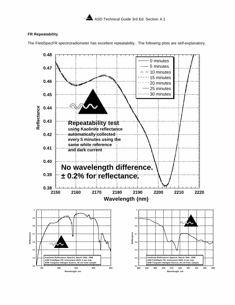
Section 4 FR Repeatability The FieldSpecFR spectroradiometer has excellent repeatability. The following plots are self-explanatory.
0.38
0.39
0.40
0.41
0.42
0.43
0.44
0.45
0.46
0.47
0.48
2150 2160 2170 2180 2190 2200 2210 2220
0 minutes5 minutes10 minutes15 minutes20 minutes25 minutes30 minutes
Wavelength (nm)
Ref
lect
ance
using Kaolinite reflectanceautomatically collectedevery 5 minutes using thesame white referenceand dark current
No wavelength difference. ± 0.2% for reflectance.
Repeatability test
0.3
0.4
0.5
0.6
0.7
0.8
0.9
1
2000 2044 2089 2133 2178 2222 2267 2311 2356 2400
Wavelength, nm
Ref
lect
ance
Kaolinite Reflectance Spectra, March 16th, 1996ASD FieldSpec FR, instrument #644, 5 sec avg.50W Tungsten Halogen Source, 30 cm from sample
0.3
0.4
0.5
0.6
0.7
0.8
0.9
1
500 1000 1500 2000 2500
Wavelength, nm
Ref
lect
ance
Kaolinite Reflectance Spectra, March 16th, 1996ASD FieldSpec FR, instrument #644, 5 sec avg.50W Tungsten Halogen Source, 30 cm from sample
ASD Technical Guide 3rd Ed. Section 4-2
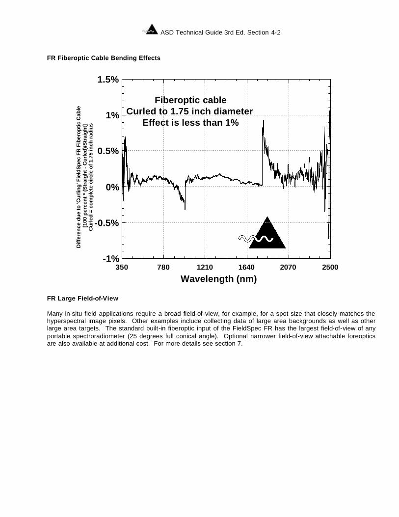
FR Fiberoptic Cable Bending Effects FR Large Field-of-View Many in-situ field applications require a broad field-of-view, for example, for a spot size that closely matches the hyperspectral image pixels. Other examples include collecting data of large area backgrounds as well as other large area targets. The standard built-in fiberoptic input of the FieldSpec FR has the largest field-of-view of any portable spectroradiometer (25 degrees full conical angle). Optional narrower field-of-view attachable foreoptics are also available at additional cost. For more details see section 7.
-1%
-0.5%
0%
0.5%
1%
1.5%
350 780 1210 1640 2070 2500
Diff
eren
ce d
ue to
'Cur
ling'
Fie
ldS
pec
FR F
iber
optic
Cab
le
[100
per
cent
* (S
trai
ght -
Cur
led)
/Str
aigh
t]C
urle
d =
com
plet
e ci
rcle
of 1
.75
inch
rad
ius
Wavelength (nm)
Fiberoptic cableCurled to 1.75 inch diameter
Effect is less than 1%
ASD Technical Guide 3rd Ed. Section 5-1
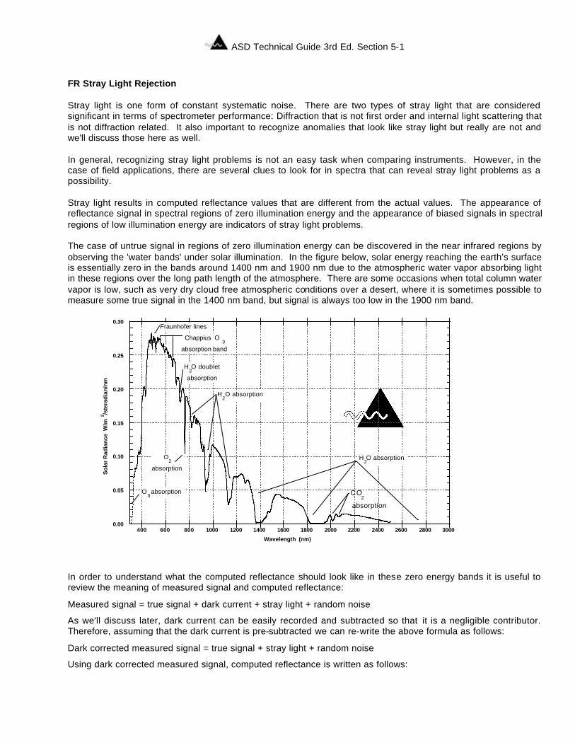
Section 5 FR Stray Light Rejection Stray light is one form of constant systematic noise. There are two types of stray light that are considered significant in terms of spectrometer performance: Diffraction that is not first order and internal light scattering that is not diffraction related. It also important to recognize anomalies that look like stray light but really are not and we'll discuss those here as well. In general, recognizing stray light problems is not an easy task when comparing instruments. However, in the case of field applications, there are several clues to look for in spectra that can reveal stray light problems as a possibility. Stray light results in computed reflectance values that are different from the actual values. The appearance of reflectance signal in spectral regions of zero illumination energy and the appearance of biased signals in spectral regions of low illumination energy are indicators of stray light problems. The case of untrue signal in regions of zero illumination energy can be discovered in the near infrared regions by observing the 'water bands' under solar illumination. In the figure below, solar energy reaching the earth’s surface is essentially zero in the bands around 1400 nm and 1900 nm due to the atmospheric water vapor absorbing light in these regions over the long path length of the atmosphere. There are some occasions when total column water vapor is low, such as very dry cloud free atmospheric conditions over a desert, where it is sometimes possible to measure some true signal in the 1400 nm band, but signal is always too low in the 1900 nm band.
In order to understand what the computed reflectance should look like in these zero energy bands it is useful to review the meaning of measured signal and computed reflectance:
Measured signal = true signal + dark current + stray light + random noise
As we'll discuss later, dark current can be easily recorded and subtracted so that it is a negligible contributor. Therefore, assuming that the dark current is pre-subtracted we can re-write the above formula as follows:
Dark corrected measured signal = true signal + stray light + random noise
Using dark corrected measured signal, computed reflectance is written as follows:
0.00
0.05
0.10
0.15
0.20
0.25
0.30
400 600 800 1000 1200 1400 1600 1800 2000 2200 2400 2600 2800 3000
Sol
ar R
adia
nce
W/m
2 /ste
radi
an/n
m
Wavelength (nm)
H2O absorption
H2O absorption
O2
absorption
Chappius O3
absorption band
H2O doublet
absorption
Fraunhofer lines
O3 absorption CO
2
absorption
ASD Technical Guide 3rd Ed. Section 5-2
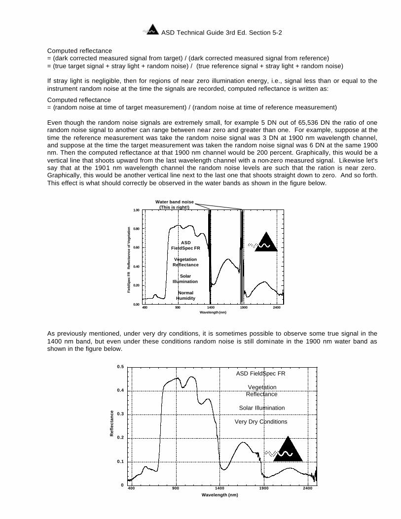
Computed reflectance = (dark corrected measured signal from target) / (dark corrected measured signal from reference) = (true target signal + stray light + random noise) / (true reference signal + stray light + random noise) If stray light is negligible, then for regions of near zero illumination energy, i.e., signal less than or equal to the instrument random noise at the time the signals are recorded, computed reflectance is written as:
Computed reflectance = (random noise at time of target measurement) / (random noise at time of reference measurement) Even though the random noise signals are extremely small, for example 5 DN out of 65,536 DN the ratio of one random noise signal to another can range between near zero and greater than one. For example, suppose at the time the reference measurement was take the random noise signal was 3 DN at 1900 nm wavelength channel, and suppose at the time the target measurement was taken the random noise signal was 6 DN at the same 1900 nm. Then the computed reflectance at that 1900 nm channel would be 200 percent. Graphically, this would be a vertical line that shoots upward from the last wavelength channel with a non-zero measured signal. Likewise let's say that at the 1901 nm wavelength channel the random noise levels are such that the ration is near zero. Graphically, this would be another vertical line next to the last one that shoots straight down to zero. And so forth. This effect is what should correctly be observed in the water bands as shown in the figure below. As previously mentioned, under very dry conditions, it is sometimes possible to observe some true signal in the 1400 nm band, but even under these conditions random noise is still dominate in the 1900 nm water band as shown in the figure below.
0.00
0.20
0.40
0.60
0.80
1.00
400 900 1400 1900 2400
Fiel
dSpe
c FR
R
efle
ctan
nce
of V
eget
atio
n
Wavelength (nm)
Water band noise(This is right!)
ASDFieldSpec FR
VegetationReflectance
SolarIllumination
NormalHumidity
0
0.1
0.2
0.3
0.4
0.5
400 900 1400 1900 2400
Ref
lect
ance
Wavelength (nm)
ASD FieldSpec FR
VegetationReflectance
Solar Illumination
Very Dry Conditions
ASD Technical Guide 3rd Ed. Section 5-3
Now, going back to the formula for computed reflectance:
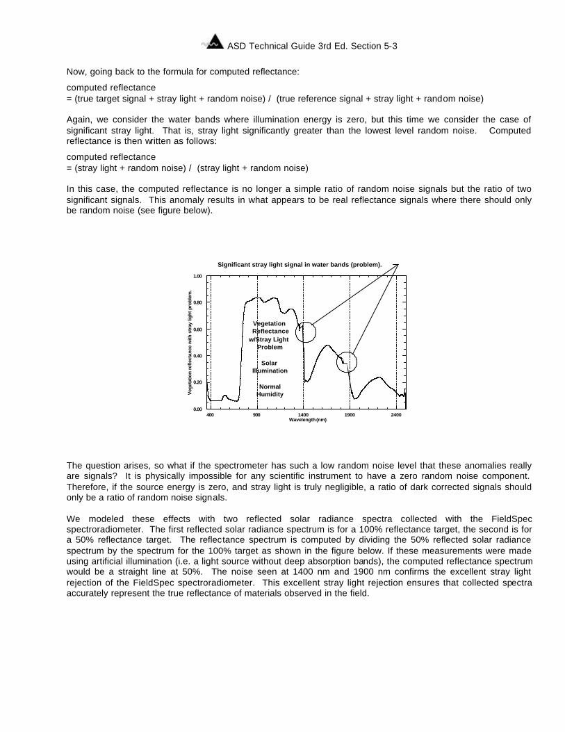
computed reflectance = (true target signal + stray light + random noise) / (true reference signal + stray light + random noise) Again, we consider the water bands where illumination energy is zero, but this time we consider the case of significant stray light. That is, stray light significantly greater than the lowest level random noise. Computed reflectance is then written as follows:
computed reflectance = (stray light + random noise) / (stray light + random noise) In this case, the computed reflectance is no longer a simple ratio of random noise signals but the ratio of two significant signals. This anomaly results in what appears to be real reflectance signals where there should only be random noise (see figure below). The question arises, so what if the spectrometer has such a low random noise level that these anomalies really are signals? It is physically impossible for any scientific instrument to have a zero random noise component. Therefore, if the source energy is zero, and stray light is truly negligible, a ratio of dark corrected signals should only be a ratio of random noise signals. We modeled these effects with two reflected solar radiance spectra collected with the FieldSpec spectroradiometer. The first reflected solar radiance spectrum is for a 100% reflectance target, the second is for a 50% reflectance target. The reflectance spectrum is computed by dividing the 50% reflected solar radiance spectrum by the spectrum for the 100% target as shown in the figure below. If these measurements were made using artificial illumination (i.e. a light source without deep absorption bands), the computed reflectance spectrum would be a straight line at 50%. The noise seen at 1400 nm and 1900 nm confirms the excellent stray light rejection of the FieldSpec spectroradiometer. This excellent stray light rejection ensures that collected spectra accurately represent the true reflectance of materials observed in the field.
0.00
0.20
0.40
0.60
0.80
1.00
400 900 1400 1900 2400
Veg
etat
ion
refle
ctan
ce w
ith s
tray
ligh
t pro
blem
.
Wavelength (nm)
Significant stray light signal in water bands (problem).
Vegetation Reflectance
w/Stray Light Problem
Solar Illumination
NormalHumidity
ASD Technical Guide 3rd Ed. Section 5-4
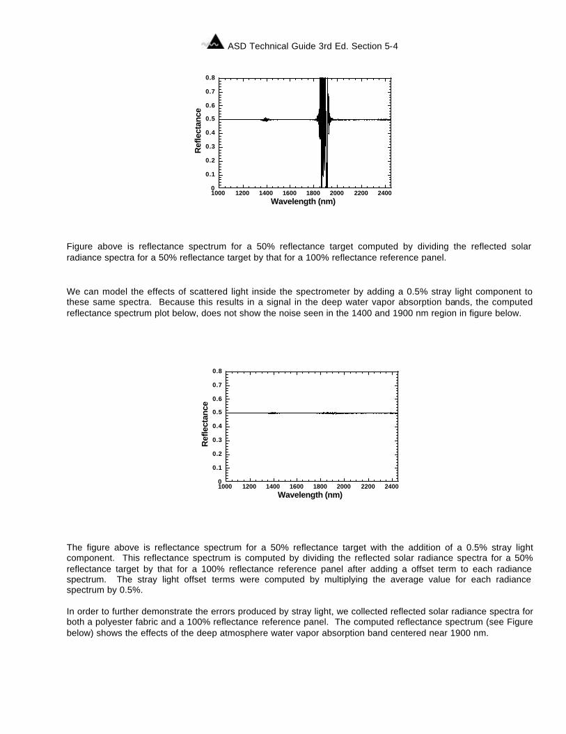
Figure above is reflectance spectrum for a 50% reflectance target computed by dividing the reflected solar radiance spectra for a 50% reflectance target by that for a 100% reflectance reference panel.
We can model the effects of scattered light inside the spectrometer by adding a 0.5% stray light component to these same spectra. Because this results in a signal in the deep water vapor absorption bands, the computed reflectance spectrum plot below, does not show the noise seen in the 1400 and 1900 nm region in figure below. The figure above is reflectance spectrum for a 50% reflectance target with the addition of a 0.5% stray light component. This reflectance spectrum is computed by dividing the reflected solar radiance spectra for a 50% reflectance target by that for a 100% reflectance reference panel after adding a offset term to each radiance spectrum. The stray light offset terms were computed by multiplying the average value for each radiance spectrum by 0.5%. In order to further demonstrate the errors produced by stray light, we collected reflected solar radiance spectra for both a polyester fabric and a 100% reflectance reference panel. The computed reflectance spectrum (see Figure below) shows the effects of the deep atmosphere water vapor absorption band centered near 1900 nm.
0
0.1
0.2
0.3
0.4
0.5
0.6
0.7
0.8
1000 1200 1400 1600 1800 2000 2200 2400R
efle
ctan
ceWavelength (nm)
0
0.1
0.2
0.3
0.4
0.5
0.6
0.7
0.8
1000 1200 1400 1600 1800 2000 2200 2400
Ref
lect
ance
Wavelength (nm)
ASD Technical Guide 3rd Ed. Section 5-5
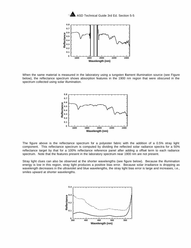
When the same material is measured in the laboratory using a tungsten filament illumination source (see Figure below), the reflectance spectrum shows absorption features in the 1900 nm region that were obscured in the spectrum collected using solar illumination. The figure above is the reflectance spectrum for a polyester fabric with the addition of a 0.5% stray light component. This reflectance spectrum is computed by dividing the reflected solar radiance spectra for a 50% reflectance target by that for a 100% reflectance reference panel after adding a offset term to each radiance spectrum. Note that the features present in the laboratory spectrum near 1900 nm are not present. Stray light clues can also be observed at the shorter wavelengths (see figure below). Because the illumination energy is low in this region, stray light produces a positive bias error. Because solar irradiance is dropping as wavelength decreases in the ultraviolet and blue wavelengths, the stray light bias error is large and increases, i.e., smiles upward at shorter wavelengths.
0
0.1
0.2
0.3
0.4
0.5
0.6
0.7
0.8
1600 1800 2000 2200 2400
Ref
lect
ance
Wavelength (nm)
0
0.1
0.2
0.3
0.4
0.5
0.6
0.7
0.8
1600 1800 2000 2200 2400
Ref
lect
ance
Wavelength (nm)
0
0.1
0.2
0.3
0.4
350 400 450 500 550
Ref
lect
ance
Wavelength (nm)
ASD Technical Guide 3rd Ed. Section 5-6
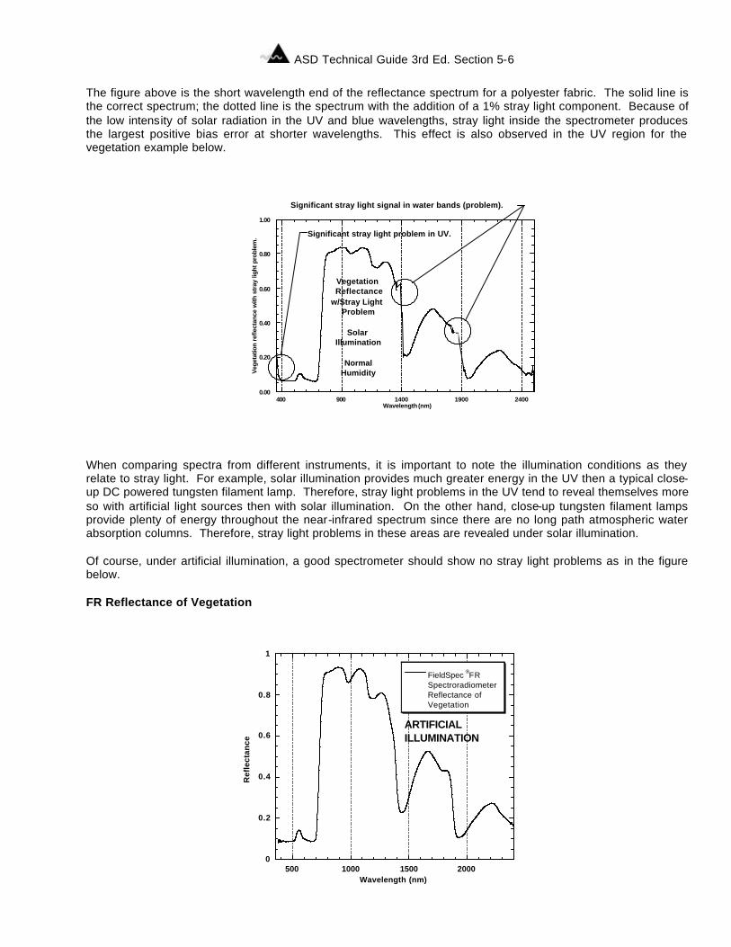
The figure above is the short wavelength end of the reflectance spectrum for a polyester fabric. The solid line is the correct spectrum; the dotted line is the spectrum with the addition of a 1% stray light component. Because of the low intensity of solar radiation in the UV and blue wavelengths, stray light inside the spectrometer produces the largest positive bias error at shorter wavelengths. This effect is also observed in the UV region for the vegetation example below.
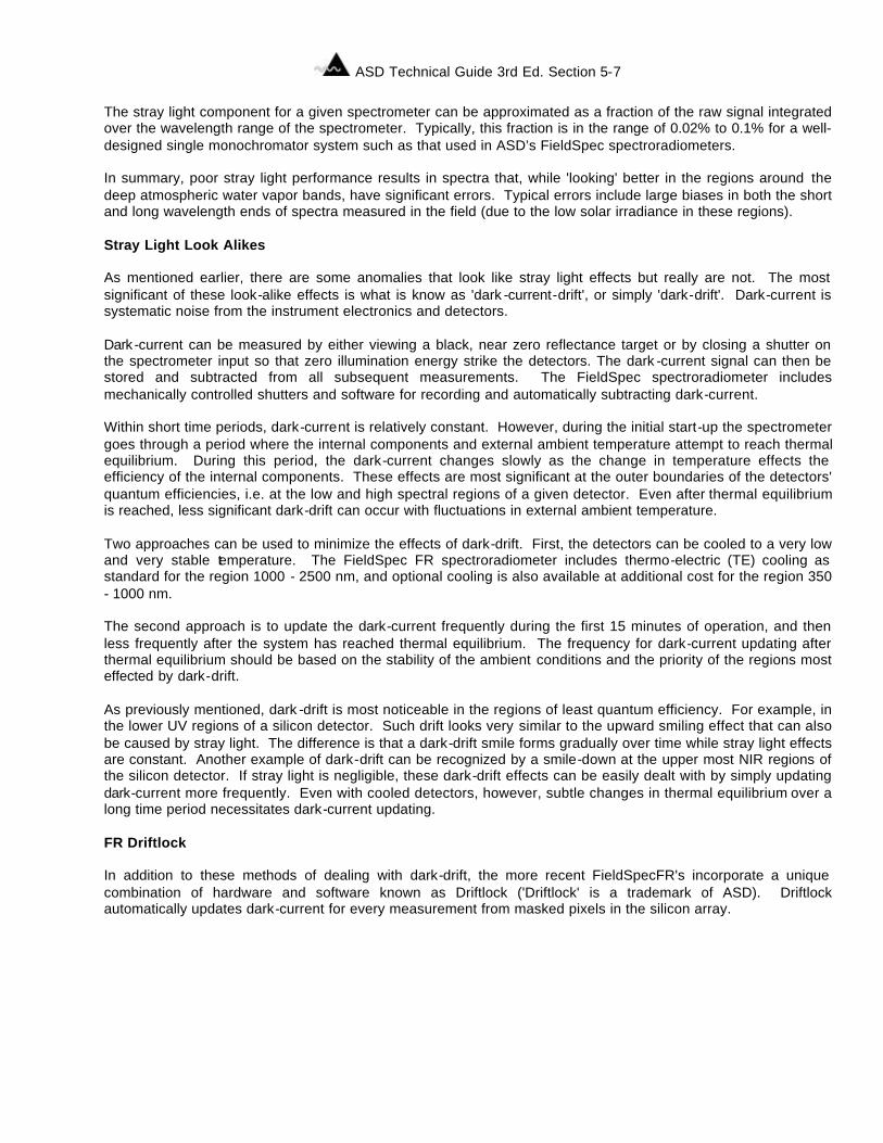
When comparing spectra from different instruments, it is important to note the illumination conditions as they relate to stray light. For example, solar illumination provides much greater energy in the UV then a typical close-up DC powered tungsten filament lamp. Therefore, stray light problems in the UV tend to reveal themselves more so with artificial light sources then with solar illumination. On the other hand, close-up tungsten filament lamps provide plenty of energy throughout the near-infrared spectrum since there are no long path atmospheric water absorption columns. Therefore, stray light problems in these areas are revealed under solar illumination. Of course, under artificial illumination, a good spectrometer should show no stray light problems as in the figure below. FR Reflectance of Vegetation
0
0.2
0.4
0.6
0.8
1
500 1000 1500 2000
FieldSpec ®FRSpectroradiometer Reflectance of Vegetation
Ref
lect
ance
Wavelength (nm)
ARTIFICIALILLUMINATION
0.00
0.20
0.40
0.60
0.80
1.00
400 900 1400 1900 2400
Veg
etat
ion
refle
ctan
ce w
ith s
tray
ligh
t pro
blem
.
Wavelength (nm)
Significant stray light signal in water bands (problem).
Vegetation Reflectance
w/Stray Light Problem
Solar Illumination
NormalHumidity
Significant stray light problem in UV.
ASD Technical Guide 3rd Ed. Section 5-7
The stray light component for a given spectrometer can be approximated as a fraction of the raw signal integrated over the wavelength range of the spectrometer. Typically, this fraction is in the range of 0.02% to 0.1% for a well-designed single monochromator system such as that used in ASD’s FieldSpec spectroradiometers. In summary, poor stray light performance results in spectra that, while 'looking' better in the regions around the deep atmospheric water vapor bands, have significant errors. Typical errors include large biases in both the short and long wavelength ends of spectra measured in the field (due to the low solar irradiance in these regions). Stray Light Look Alikes As mentioned earlier, there are some anomalies that look like stray light effects but really are not. The most significant of these look-alike effects is what is know as 'dark -current-drift', or simply 'dark-drift'. Dark-current is systematic noise from the instrument electronics and detectors. Dark -current can be measured by either viewing a black, near zero reflectance target or by closing a shutter on the spectrometer input so that zero illumination energy strike the detectors. The dark -current signal can then be stored and subtracted from all subsequent measurements. The FieldSpec spectroradiometer includes mechanically controlled shutters and software for recording and automatically subtracting dark-current. Within short time periods, dark-current is relatively constant. However, during the initial start-up the spectrometer goes through a period where the internal components and external ambient temperature attempt to reach thermal equilibrium. During this period, the dark-current changes slowly as the change in temperature effects the efficiency of the internal components. These effects are most significant at the outer boundaries of the detectors' quantum efficiencies, i.e. at the low and high spectral regions of a given detector. Even after thermal equilibrium is reached, less significant dark-drift can occur with fluctuations in external ambient temperature. Two approaches can be used to minimize the effects of dark-drift. First, the detectors can be cooled to a very low and very stable temperature. The FieldSpec FR spectroradiometer includes thermo-electric (TE) cooling as standard for the region 1000 - 2500 nm, and optional cooling is also available at additional cost for the region 350 - 1000 nm. The second approach is to update the dark-current frequently during the first 15 minutes of operation, and then less frequently after the system has reached thermal equilibrium. The frequency for dark-current updating after thermal equilibrium should be based on the stability of the ambient conditions and the priority of the regions most effected by dark-drift. As previously mentioned, dark -drift is most noticeable in the regions of least quantum efficiency. For example, in the lower UV regions of a silicon detector. Such drift looks very similar to the upward smiling effect that can also be caused by stray light. The difference is that a dark-drift smile forms gradually over time while stray light effects are constant. Another example of dark-drift can be recognized by a smile-down at the upper most NIR regions of the silicon detector. If stray light is negligible, these dark-drift effects can be easily dealt with by simply updating dark-current more frequently. Even with cooled detectors, however, subtle changes in thermal equilibrium over a long time period necessitates dark-current updating. FR Driftlock In addition to these methods of dealing with dark-drift, the more recent FieldSpecFR's incorporate a unique combination of hardware and software known as Driftlock ('Driftlock' is a trademark of ASD). Driftlock automatically updates dark-current for every measurement from masked pixels in the silicon array.

ASD Technical Guide 3rd Ed. Section 5-8
ASD Technical Guide 3rd Ed. Section 6-1
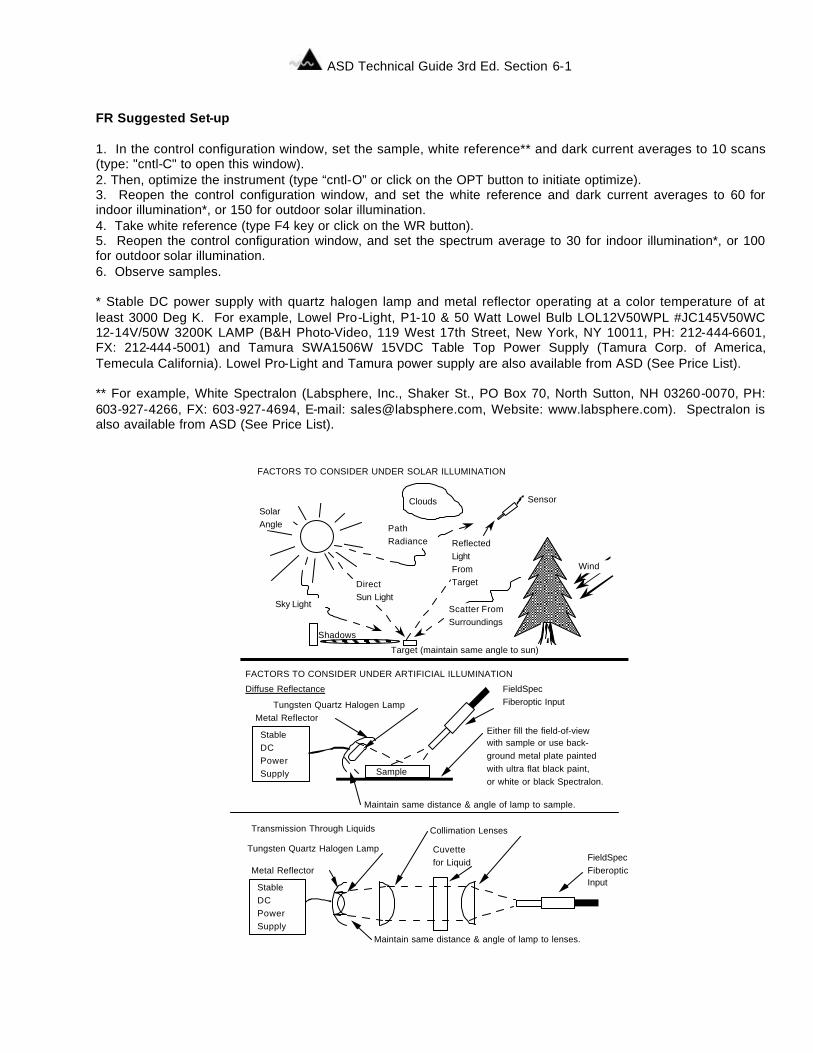
Section 6 FR Suggested Set-up 1. In the control configuration window, set the sample, white reference** and dark current averages to 10 scans (type: "cntl-C" to open this window). 2. Then, optimize the instrument (type “cntl-O” or click on the OPT button to initiate optimize). 3. Reopen the control configuration window, and set the white reference and dark current averages to 60 for indoor illumination*, or 150 for outdoor solar illumination. 4. Take white reference (type F4 key or click on the WR button). 5. Reopen the control configuration window, and set the spectrum average to 30 for indoor illumination*, or 100 for outdoor solar illumination. 6. Observe samples. * Stable DC power supply with quartz halogen lamp and metal reflector operating at a color temperature of at least 3000 Deg K. For example, Lowel Pro-Light, P1-10 & 50 Watt Lowel Bulb LOL12V50WPL #JC145V50WC 12-14V/50W 3200K LAMP (B&H Photo-Video, 119 West 17th Street, New York, NY 10011, PH: 212-444-6601, FX: 212-444-5001) and Tamura SWA1506W 15VDC Table Top Power Supply (Tamura Corp. of America, Temecula California). Lowel Pro-Light and Tamura power supply are also available from ASD (See Price List). ** For example, White Spectralon (Labsphere, Inc., Shaker St., PO Box 70, North Sutton, NH 03260-0070, PH: 603-927-4266, FX: 603-927-4694, E-mail: [email protected], Website: www.labsphere.com). Spectralon is also available from ASD (See Price List).
StableDCPowerSupply
Metal Reflector
Collimation Lenses
Cuvettefor Liquid FieldSpec
FiberopticInput
Transmission Through Liquids
Tungsten Quartz Halogen Lamp
Diffuse Reflectance
StableDCPowerSupply
Metal ReflectorTungsten Quartz Halogen Lamp
Sample
Either fill the field-of-viewwith sample or use back-ground metal plate paintedwith ultra flat black paint,or white or black Spectralon.
FieldSpecFiberoptic Input
Scatter FromSurroundings
Sky Light
Target (maintain same angle to sun)
PathRadiance
DirectSun Light
ReflectedLightFromTarget
Sensor
Wind
CloudsSolarAngle
FACTORS TO CONSIDER UNDER SOLAR ILLUMINATION
Shadows
FACTORS TO CONSIDER UNDER ARTIFICIAL ILLUMINATION
Maintain same distance & angle of lamp to lenses.
Maintain same distance & angle of lamp to sample.
ASD Technical Guide 3rd Ed. Section 6-2
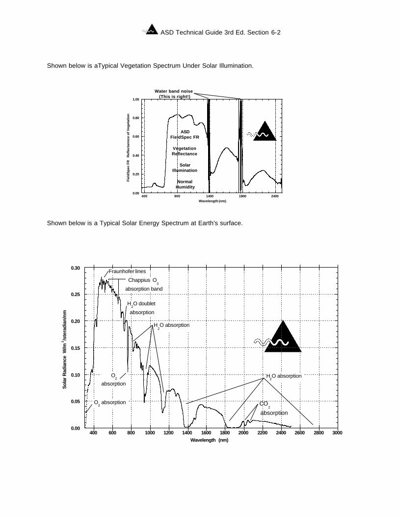
Shown below is aTypical Vegetation Spectrum Under Solar Illumination. Shown below is a Typical Solar Energy Spectrum at Earth's surface.
0.00
0.20
0.40
0.60
0.80
1.00
400 900 1400 1900 2400
Fiel
dSpe
c FR
R
efle
ctan
nce
of V
eget
atio
n
Wavelength (nm)
Water band noise(This is right!)
ASDFieldSpec FR
VegetationReflectance
SolarIllumination
NormalHumidity
0.00
0.05
0.10
0.15
0.20
0.25
0.30
400 600 800 1000 1200 1400 1600 1800 2000 2200 2400 2600 2800 3000
Sol
ar R
adia
nce
W/m
2/s
tera
dian
/nm
Wavelength (nm)
H2O absorption
H2O absorption
O2
absorption
Chappius O3
absorption band
H2O doublet
absorption
Fraunhofer lines
O3 absorption CO
2
absorption
ASD Technical Guide 3rd Ed. Section 6-3
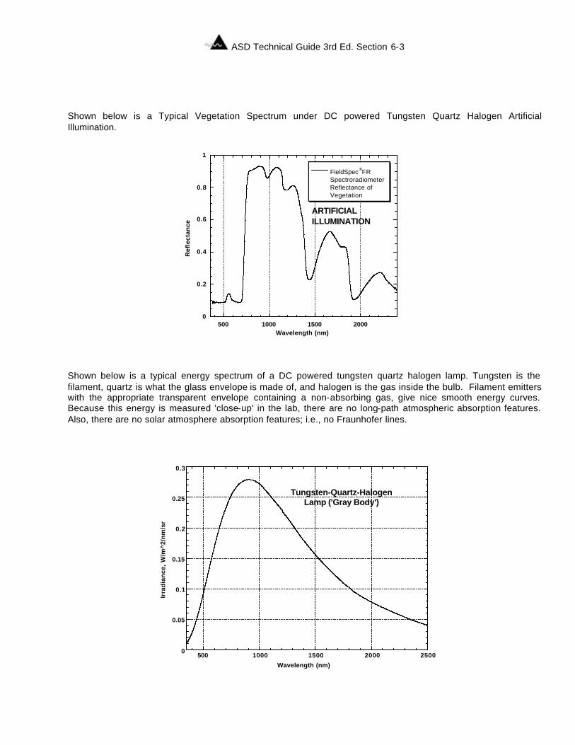
Shown below is a Typical Vegetation Spectrum under DC powered Tungsten Quartz Halogen Artificial Illumination. Shown below is a typical energy spectrum of a DC powered tungsten quartz halogen lamp. Tungsten is the filament, quartz is what the glass envelope is made of, and halogen is the gas inside the bulb. Filament emitters with the appropriate transparent envelope containing a non-absorbing gas, give nice smooth energy curves. Because this energy is measured 'close-up' in the lab, there are no long-path atmospheric absorption features. Also, there are no solar atmosphere absorption features; i.e., no Fraunhofer lines.
0
0.2
0.4
0.6
0.8
1
500 1000 1500 2000
FieldSpec®FRSpectroradiometer Reflectance of Vegetation
Ref
lect
ance
Wavelength (nm)
ARTIFICIALILLUMINATION
0
0.05
0.1
0.15
0.2
0.25
0.3
500 1000 1500 2000 2500
Tungsten-Quartz-HalogenLamp ('Gray Body')
Irra
dia
nce
, W
/m^2
/nm
/sr
Wavelength (nm)
ASD Technical Guide 3rd Ed. Section 6-4
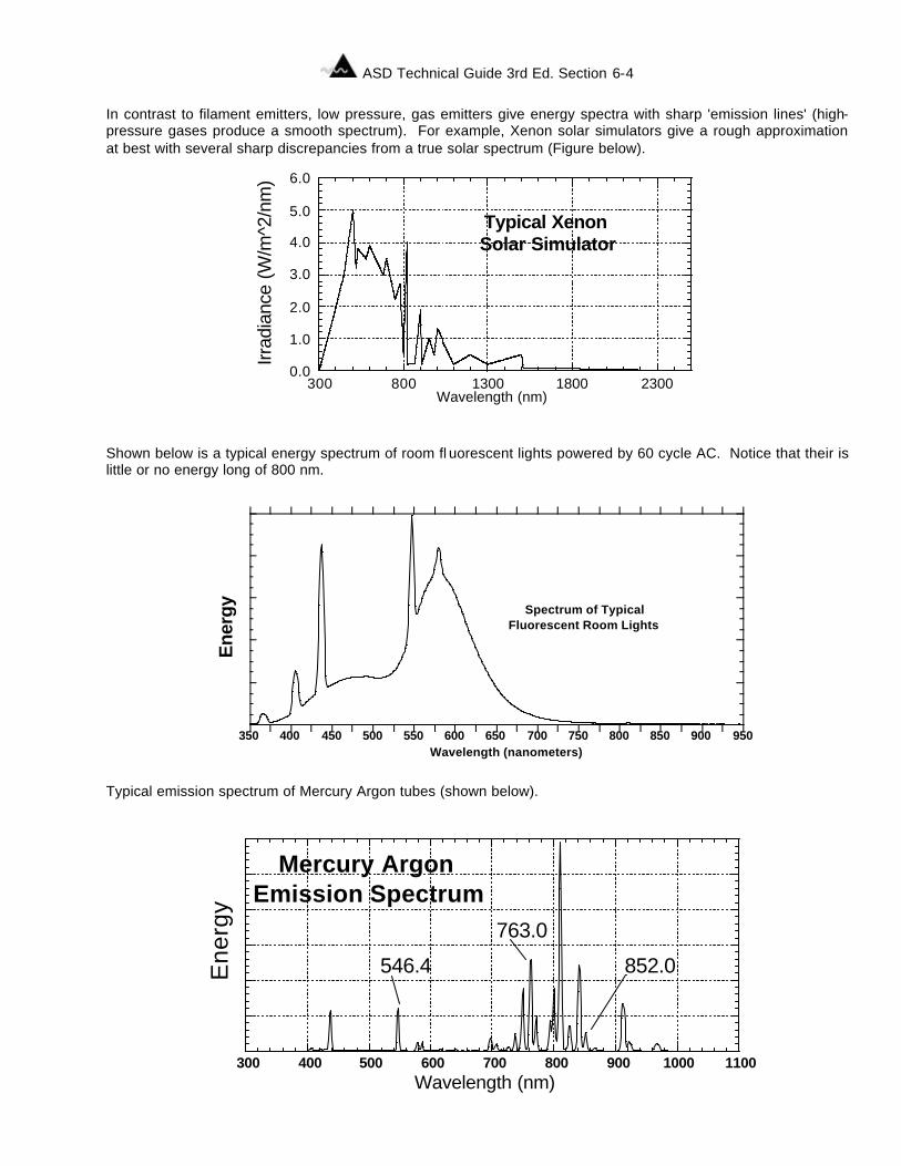
In contrast to filament emitters, low pressure, gas emitters give energy spectra with sharp 'emission lines' (high-pressure gases produce a smooth spectrum). For example, Xenon solar simulators give a rough approximation at best with several sharp discrepancies from a true solar spectrum (Figure below). Shown below is a typical energy spectrum of room fl uorescent lights powered by 60 cycle AC. Notice that their is little or no energy long of 800 nm. Typical emission spectrum of Mercury Argon tubes (shown below).
350 400 450 500 550 600 650 700 750 800 850 900 950Wavelength (nanometers)
Ene
rgy
Spectrum of TypicalFluorescent Room Lights
300 400 500 600 700 800 900 1000 1100
Mercury Argon Emission Spectrum
Ene
rgy
Wavelength (nm)
546.4
763.0
852.0
0.0
1.0
2.0
3.0
4.0
5.0
6.0
300 800 1300 1800 2300
Typical XenonSolar Simulator
Irrad
ianc
e (W
/m^2
/nm
)
Wavelength (nm)
ASD Technical Guide 3rd Ed. Section 6-5
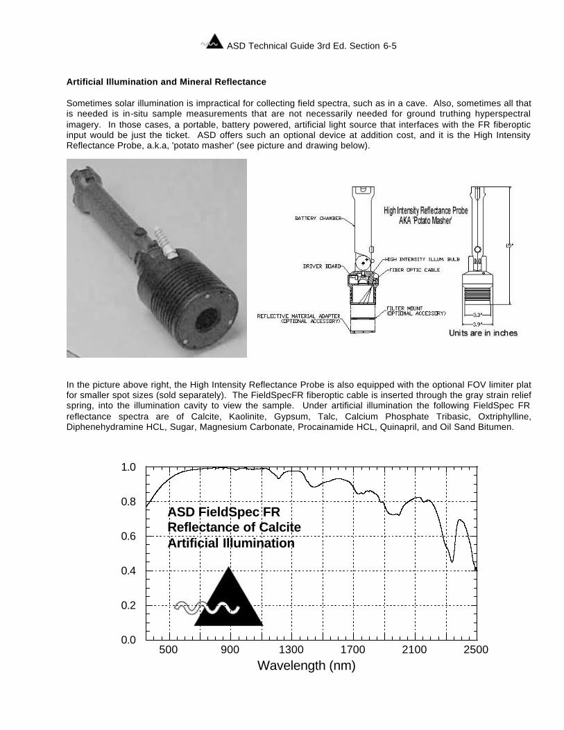
Artificial Illumination and Mineral Reflectance Sometimes solar illumination is impractical for collecting field spectra, such as in a cave. Also, sometimes all that is needed is in-situ sample measurements that are not necessarily needed for ground truthing hyperspectral imagery. In those cases, a portable, battery powered, artificial light source that interfaces with the FR fiberoptic input would be just the ticket. ASD offers such an optional device at addition cost, and it is the High Intensity Reflectance Probe, a.k.a, 'potato masher' (see picture and drawing below).
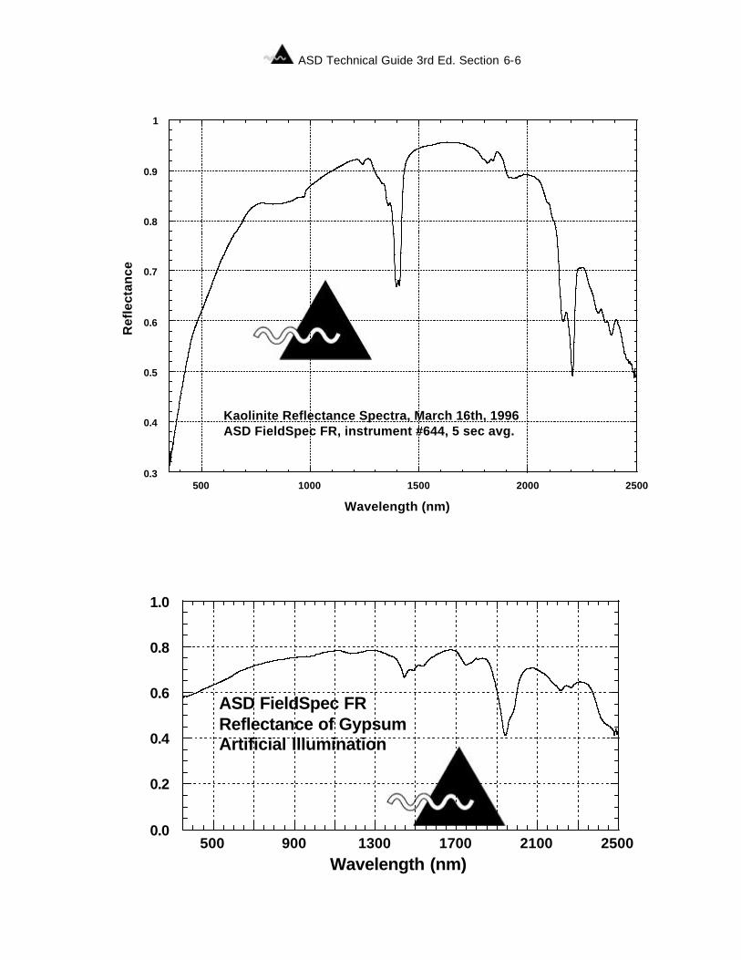
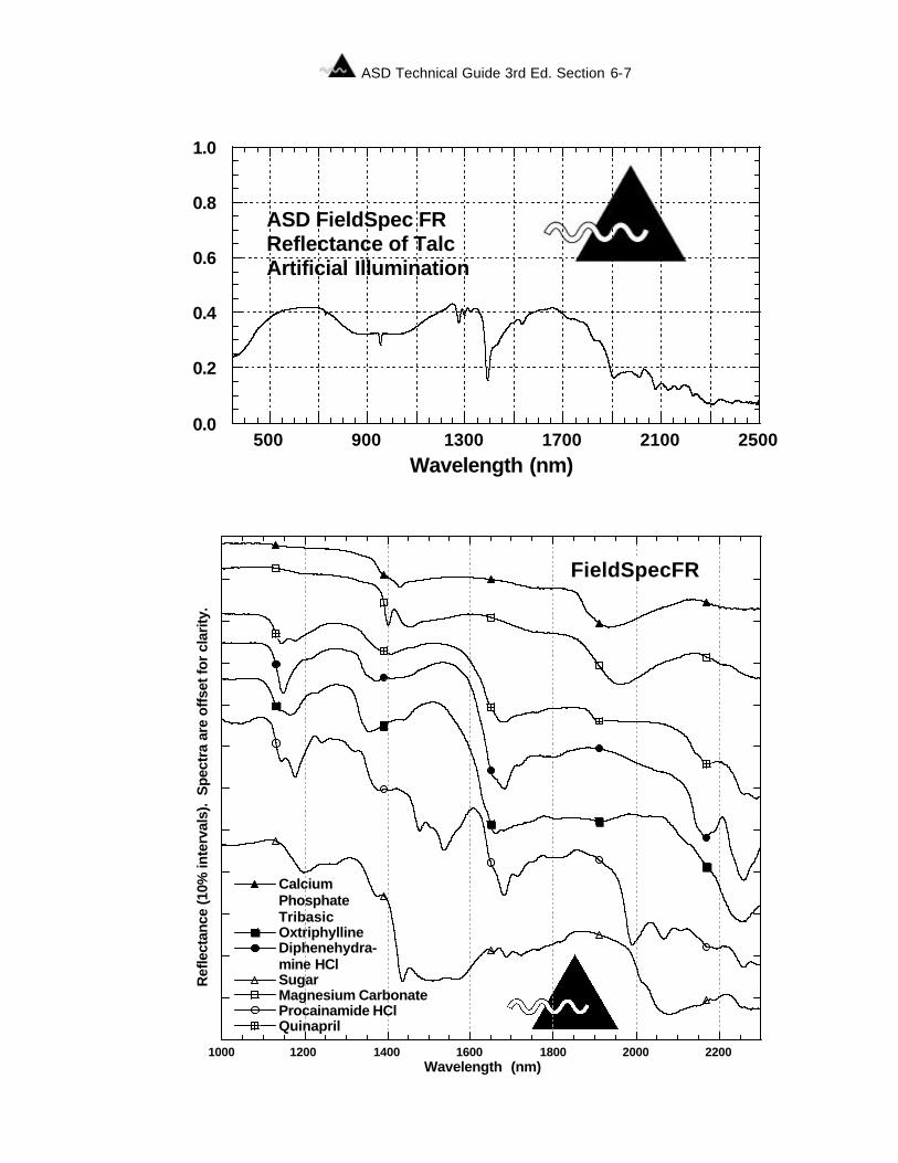
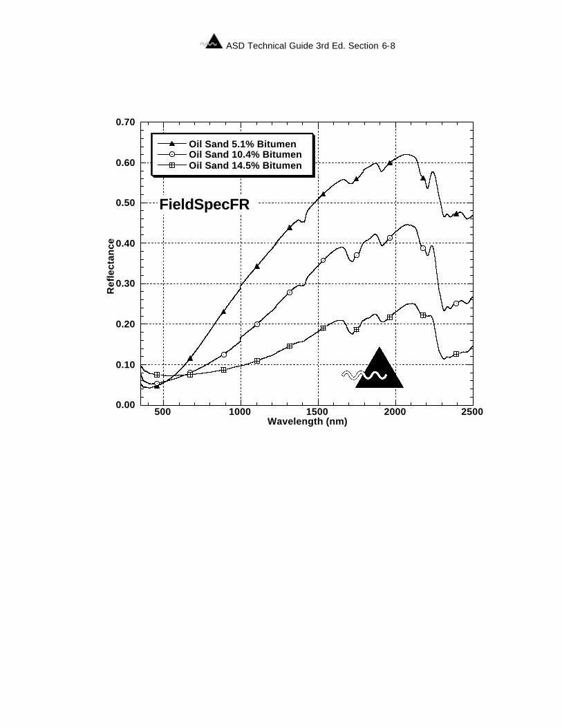
In the picture above right, the High Intensity Reflectance Probe is also equipped with the optional FOV limiter plat for smaller spot sizes (sold separately). The FieldSpecFR fiberoptic cable is inserted through the gray strain relief spring, into the illumination cavity to view the sample. Under artificial illumination the following FieldSpec FR reflectance spectra are of Calcite, Kaolinite, Gypsum, Talc, Calcium Phosphate Tribasic, Oxtriphylline, Diphenehydramine HCL, Sugar, Magnesium Carbonate, Procainamide HCL, Quinapril, and Oil Sand Bitumen.
0.0
0.2
0.4
0.6
0.8
1.0
500 900 1300 1700 2100 2500Wavelength (nm)
ASD FieldSpec FRReflectance of CalciteArtificial Illumination
ASD Technical Guide 3rd Ed. Section 6-6
0.3
0.4
0.5
0.6
0.7
0.8
0.9
1
500 1000 1500 2000 2500
Wavelength (nm)
Ref
lect
ance
Kaolinite Reflectance Spectra, March 16th, 1996ASD FieldSpec FR, instrument #644, 5 sec avg.
0.0
0.2
0.4
0.6
0.8
1.0
500 900 1300 1700 2100 2500Wavelength (nm)
ASD FieldSpec FRReflectance of GypsumArtificial Illumination
ASD Technical Guide 3rd Ed. Section 6-7
0.0
0.2
0.4
0.6
0.8
1.0
500 900 1300 1700 2100 2500Wavelength (nm)
ASD FieldSpec FRReflectance of TalcArtificial Illumination
Calcium Phosphate TribasicOxtriphyllineDiphenehydra-mine HClSugarMagnesium CarbonateProcainamide HClQuinapril
1000 1200 1400 1600 1800 2000 2200
Ref
lect
ance
(10%
inte
rval
s).
Spe
ctra
are
off
set f
or c
lari
ty.
Wavelength (nm)
FieldSpecFR
ASD Technical Guide 3rd Ed. Section 6-8
0.00
0.10
0.20
0.30
0.40
0.50
0.60
0.70
500 1000 1500 2000 2500
Oil Sand 5.1% BitumenOil Sand 10.4% BitumenOil Sand 14.5% Bitumen
Ref
lect
ance
Wavelength (nm)
FieldSpecFR
ASD Technical Guide 3rd Ed. Section 7-1
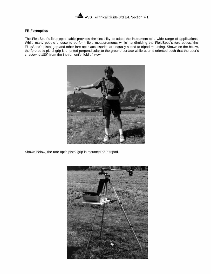
Section 7 FR Foreoptics The FieldSpec's fiber optic cable provides the flexibility to adapt the instrument to a wide range of applications. While many people choose to perform field measurements while handholding the FieldSpec's fore optics, the FieldSpec's pistol grip and other fore optic accessories are equally suited to tripod mounting. Shown on the below, the fore optic pistol grip is oriented perpendicular to the ground surface while user is oriented such that the user's shadow is 180° from the instrument's field-of-view.
Shown below, the fore optic pistol grip is mounted on a tripod.
ASD Technical Guide 3rd Ed. Section 7-2
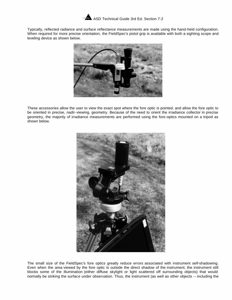
Typically, reflected radiance and surface reflectance measurements are made using the hand-held configuration. When required for more precise orientation, the FieldSpec's pistol grip is available with both a sighting scope and leveling device as shown below.
These accessories allow the user to view the exact spot where the fore optic is pointed, and allow the fore optic to be oriented in precise, nadir-viewing, geometry. Because of the need to orient the irradiance collector in precise geometry, the majority of irradiance measurements are performed using the fore-optics mounted on a tripod as shown below.
The small size of the FieldSpec's fore optics greatly reduce errors associated with instrument self-shadowing. Even when the area viewed by the fore optic is outside the direct shadow of the instrument, the instrument still blocks some of the illumination (either diffuse skylight or light scattered off surrounding objects) that would normally be striking the surface under observation. Thus, the instrument (as well as other objects -- including the
ASD Technical Guide 3rd Ed. Section 7-3
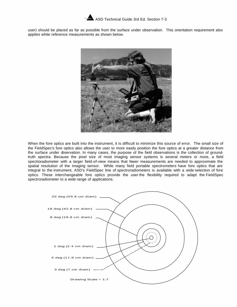
user) should be placed as far as possible from the surface under observation. This orientation requirement also applies white reference measurements as shown below.
When the fore optics are built into the instrument, it is difficult to minimize this source of error. The small size of the FieldSpec's fore optics also allows the user to more easily position the fore optics at a greater distance from the surface under observation. In many cases, the purpose of the field observations is the collection of ground-truth spectra. Because the pixel size of most imaging sensor systems is several meters or more, a field spectroradiometer with a larger field-of-view means that fewer measurements are needed to approximate the spatial resolution of the imaging sensor. While many field portable spectrometers have fore optics that are integral to the instrument, ASD's FieldSpec line of spectroradiometers is available with a wide selection of fore optics. These interchangeable fore optics provide the user the flexibility required to adapt the FieldSpec spectroradiometer to a wide range of applications.
25 deg (59.9 cm diam)
18 deg (42.8 cm diam)
8 deg (18.8 cm diam)
5 deg (11.8 cm diam)
3 deg (7 cm diam)
1 deg (2.4 cm diam)
Drawing Scale = 1:7
ASD Technical Guide 3rd Ed. Section 7-4
The figure above shows the available fields-of-view (FOV) for the FieldSpec FR with an instrument fore optic height of 135 cm. The dashed circle represents the FOV of a non-ASD instrument with a fixed 3° FOV. The solid circles are for ASD's FieldSpec FR. The largest circle is the FOV of the FieldSpec's standard built-in fiberoptic cable, with optional foreoptics providing 1°, 5°, 8°, or 18°. Fore optics covering approximately the same range of angular FOVs are available for the other FieldSpec instruments. Irradiance Observations ASD has several types of fore optic for irradiance measurements. These include:
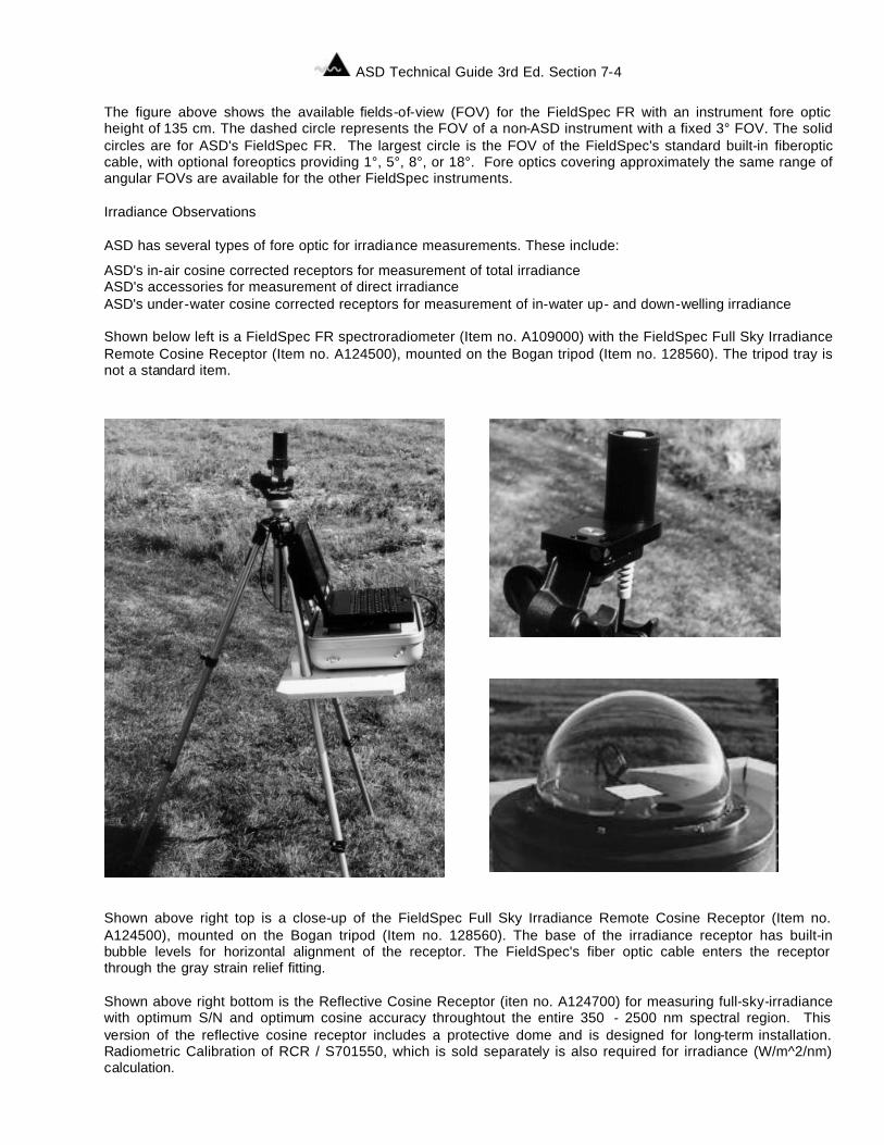
ASD's in-air cosine corrected receptors for measurement of total irradiance ASD's accessories for measurement of direct irradiance ASD's under-water cosine corrected receptors for measurement of in-water up- and down-welling irradiance Shown below left is a FieldSpec FR spectroradiometer (Item no. A109000) with the FieldSpec Full Sky Irradiance Remote Cosine Receptor (Item no. A124500), mounted on the Bogan tripod (Item no. 128560). The tripod tray is not a standard item.
Shown above right top is a close-up of the FieldSpec Full Sky Irradiance Remote Cosine Receptor (Item no. A124500), mounted on the Bogan tripod (Item no. 128560). The base of the irradiance receptor has built-in bubble levels for horizontal alignment of the receptor. The FieldSpec's fiber optic cable enters the receptor through the gray strain relief fitting. Shown above right bottom is the Reflective Cosine Receptor (iten no. A124700) for measuring full-sky-irradiance with optimum S/N and optimum cosine accuracy throughtout the entire 350 - 2500 nm spectral region. This version of the reflective cosine receptor includes a protective dome and is designed for long-term installation. Radiometric Calibration of RCR / S701550, which is sold separately is also required for irradiance (W/m^2/nm) calculation.
ASD Technical Guide 3rd Ed. Section 7-5
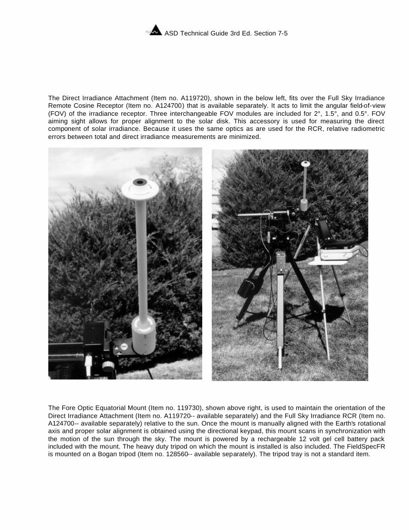
The Direct Irradiance Attachment (Item no. A119720), shown in the below left, fits over the Full Sky Irradiance Remote Cosine Receptor (Item no. A124700) that is available separately. It acts to limit the angular field-of-view (FOV) of the irradiance receptor. Three interchangeable FOV modules are included for 2°, 1.5°, and 0.5°. FOV aiming sight allows for proper alignment to the solar disk. This accessory is used for measuring the direct component of solar irradiance. Because it uses the same optics as are used for the RCR, relative radiometric errors between total and direct irradiance measurements are minimized.
The Fore Optic Equatorial Mount (Item no. 119730), shown above right, is used to maintain the orientation of the Direct Irradiance Attachment (Item no. A119720-- available separately) and the Full Sky Irradiance RCR (Item no. A124700-- available separately) relative to the sun. Once the mount is manually aligned with the Earth's rotational axis and proper solar alignment is obtained using the directional keypad, this mount scans in synchronization with the motion of the sun through the sky. The mount is powered by a rechargeable 12 volt gel cell battery pack included with the mount. The heavy duty tripod on which the mount is installed is also included. The FieldSpecFR is mounted on a Bogan tripod (Item no. 128560-- available separately). The tripod tray is not a standard item.

ASD Technical Guide 3rd Ed. Section 7-6
ASD Technical Guide 3rd Ed. Section 8-1
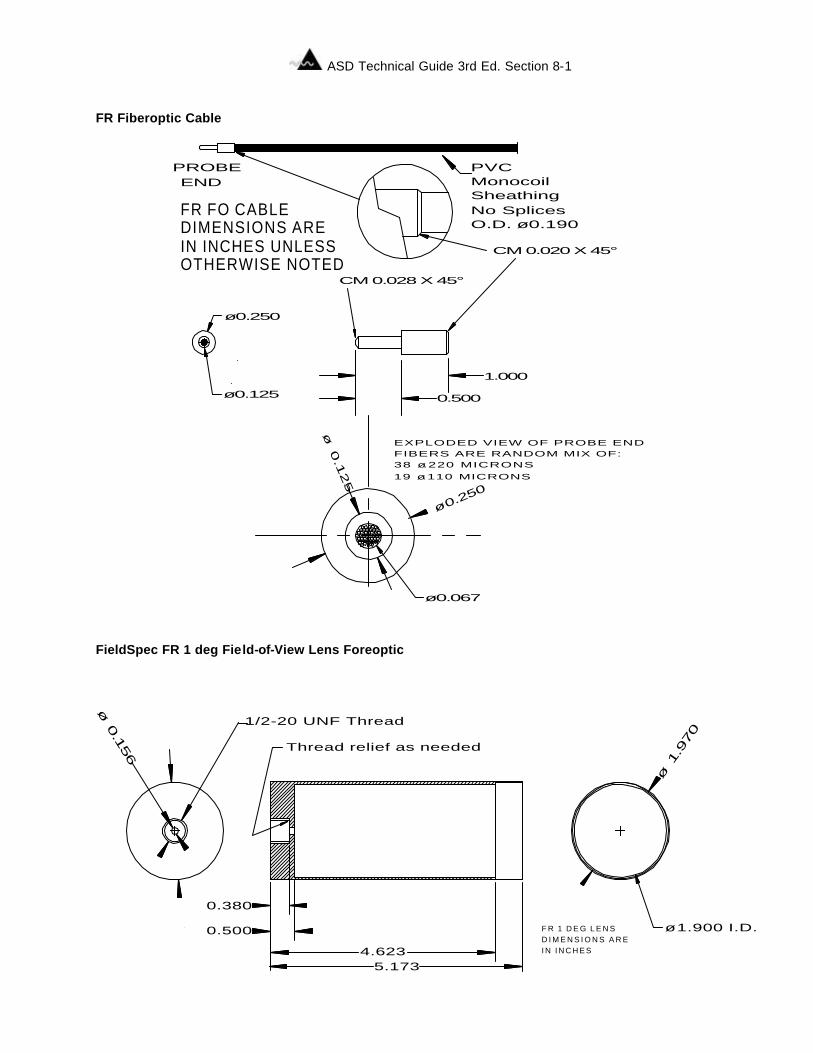
Section 8 FR Fiberoptic Cable
FieldSpec FR 1 deg Field-of-View Lens Foreoptic
CM 0.020 X 45°
PVCMonocoil SheathingNo Splices O.D. ø 0.190
ø 0.125
ø 0.250
1.000
0.500
CM 0.028 X 45°
PROBEEND
EXPLODED VIEW OF PROBE ENDFIBERS ARE RANDOM MIX OF:38 ø.220 MICRONS19 ø.110 MICRONS
ø
0.250ø
0.1
25
ø 0.067
FR FO CABLEDIMENSIONS ARE IN INCHES UNLESSOTHERWISE NOTED
ø
1.9
70
1/2-20 UNF Thread
ø
2.000
ø 0
.156
0.380
0.500
4.6235.173
Thread relief as needed
ø 1.900 I.D.F R 1 D E G L E N SD I M E N S I O N S A R EI N I N C H E S
ASD Technical Guide 3rd Ed. Section 8-2
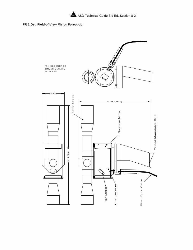
FR 1 Deg Field-of-View Mirror Foreoptic
M2
Fib
er
Op
tic C
ab
le
1° M
irro
r F
OV
45
° M
irro
r
Co
nca
ve
Mir
ror
Tri
po
d M
ou
nta
ble
Gri
p
Rif
le S
co
pe
12
.25
[31
.1]
2.75
10.00[25.4]
F R 1 D E G M I R R O RD I M E N S I O N S A R E I N I N C H E S
ASD Technical Guide 3rd Ed. Section 8-3
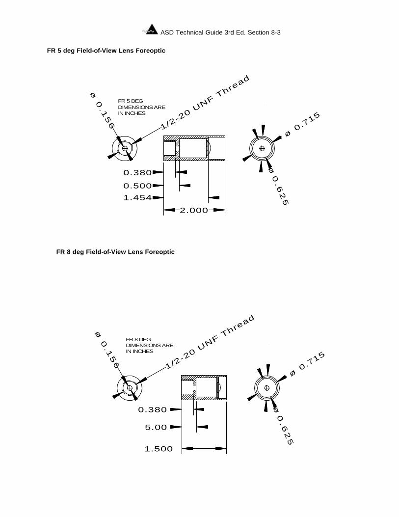
FR 5 deg Field-of-View Lens Foreoptic
FR 8 deg Field-of-View Lens Foreoptic
FR 5 DEGDIMENSIONS ARE IN INCHES
ø 0
.15
6
1/2-2
0 UNF T
hread
ø
0.
81
0
ø 0
.715
ø 0.6
25
0.380
0.500
1.454
2.000
FR 8 DEGDIMENSIONS AREIN INCHES
ø 0
.15
6
1/2-2
0 UNF T
hread
ø
0.
81
0
ø 0
.715
ø 0.6
25
0.380
5.00
1.500
ASD Technical Guide 3rd Ed. Section 8-4
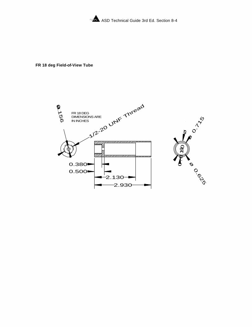
FR 18 deg Field-of-View Tube
FR 18 DEGDIMENSIONS AREIN INCHES
0.3800.500
2.130
2.930
1/2-2
0 UNF T
hread
ø
0.1
56
ø
0.8
10
ø 0
.715
ø 0
.625
ASD Technical Guide 3rd Ed. Section 8-5
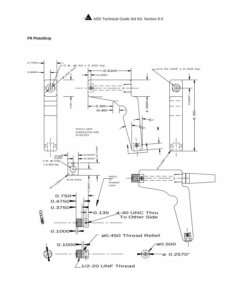
FR PistolGrip
End View
0.6443" 0.7
700"
0.3
850"
0.3222"
2.610
C.B. ø0.375
x 0.450 Dp.
0.5
000"
1.0
0
1.0
0
4.3
0
0.1650"
1/2-20 UNF x 0.450 Dp.C .B . ø0 .50 x 0 .300 Dp .
5°
15°
0.3250"0.3850"
0.7700"
1.500.40
ø0.2
60 Thru
R 0
.1250"
R 0
.1250
-0.000+0.003
ø 0.2570"
ø
0.1260
0.3750
0.1000
0.4750
0.1000
ø 0.450 Thread Relief
4-40 UNC ThruTo Other Side
1/2-20 UNF Thread
ø 0.500
0.750
0.135
detai ls
ofthreadedinsert
PISTOL GRIPDIMENSIONS ARE IN INCHES
ASD Technical Guide 3rd Ed. Section 8-6
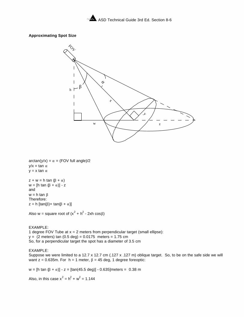
Approximating Spot Size
α
x
y
FOV
z
βh
w
arctan(y/x) = α = (FOV full angle)/2 y/x = tan α y = x tan α z + w = h tan (β + α) w = [h tan (β + α)] - z and w = h tan β Therefore: z = h [tan(β)+ tan(β + α)] Also w = square root of (x2 + h2 - 2xh cosβ) EXAMPLE: 1 degree FOV Tube at x = 2 meters from perpendicular target (small ellipse): y = (2 meters) tan (0.5 deg) = 0.0175 meters = 1.75 cm So, for a perpendicular target the spot has a diameter of 3.5 cm EXAMPLE: Suppose we were limited to a 12.7 x 12.7 cm (.127 x .127 m) oblique target. So, to be on the safe side we will want z = 0.635m. For h = 1 meter, β = 45 deg, 1 degree foreoptic: w = [h tan (β + α)] - z = [tan(45.5 deg)] - 0.635]meters = 0.38 m Also, in this case x2 = h2 + w2 = 1.144
ASD Technical Guide 3rd Ed. Section 9-1
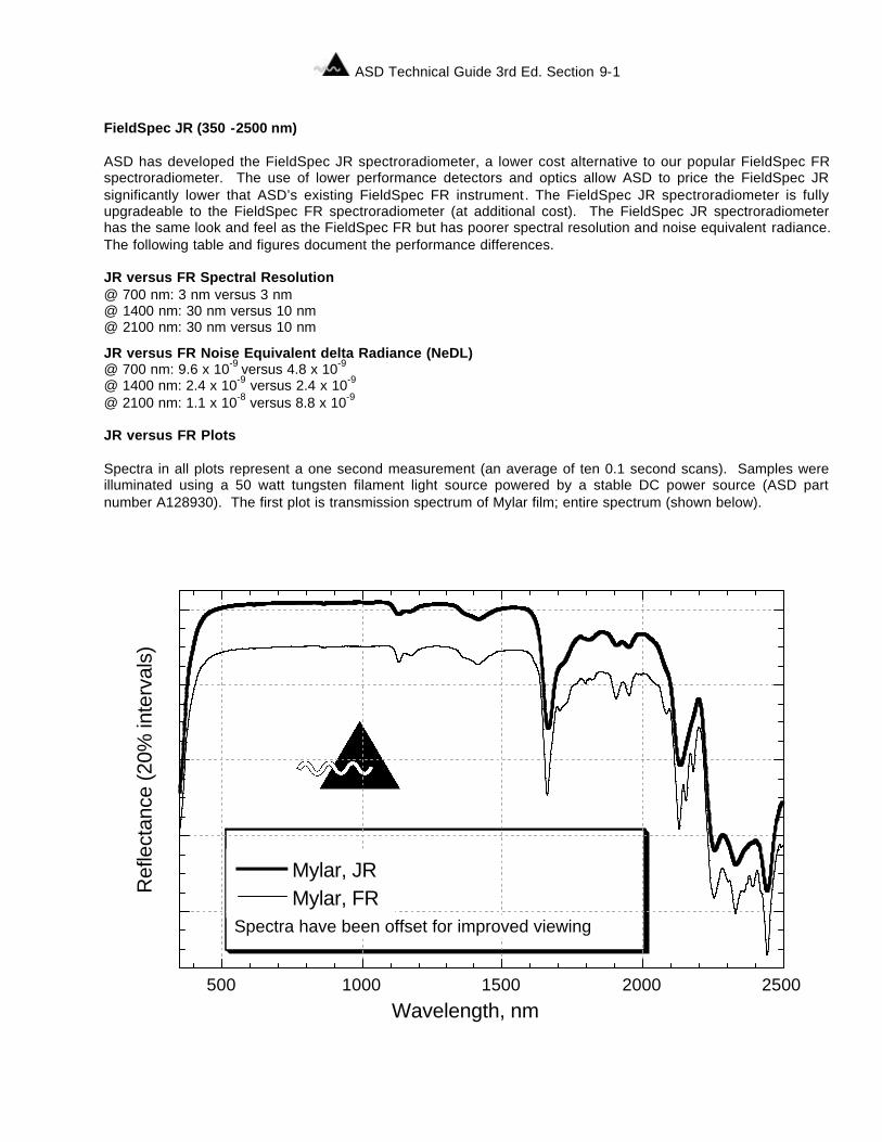
Section 9 FieldSpec JR (350 -2500 nm) ASD has developed the FieldSpec JR spectroradiometer, a lower cost alternative to our popular FieldSpec FR spectroradiometer. The use of lower performance detectors and optics allow ASD to price the FieldSpec JR significantly lower that ASD’s existing FieldSpec FR instrument. The FieldSpec JR spectroradiometer is fully upgradeable to the FieldSpec FR spectroradiometer (at additional cost). The FieldSpec JR spectroradiometer has the same look and feel as the FieldSpec FR but has poorer spectral resolution and noise equivalent radiance. The following table and figures document the performance differences. JR versus FR Spectral Resolution @ 700 nm: 3 nm versus 3 nm @ 1400 nm: 30 nm versus 10 nm @ 2100 nm: 30 nm versus 10 nm
JR versus FR Noise Equivalent delta Radiance (NeDL) @ 700 nm: 9.6 x 10⁻⁹ versus 4.8 x 10⁻⁹ @ 1400 nm: 2.4 x 10⁻⁹ versus 2.4 x 10⁻⁹ @ 2100 nm: 1.1 x 10⁻⁸ versus 8.8 x 10⁻⁹
JR versus FR Plots Spectra in all plots represent a one second measurement (an average of ten 0.1 second scans). Samples were illuminated using a 50 watt tungsten filament light source powered by a stable DC power source (ASD part number A128930). The first plot is transmission spectrum of Mylar film; entire spectrum (shown below).
500 1000 1500 2000 2500
Mylar, JRMylar, FRR
efle
ctan
ce (2
0% in
terv
als)
Wavelength, nm
Spectra have been offset for improved viewing
ASD Technical Guide 3rd Ed. Section 9-2
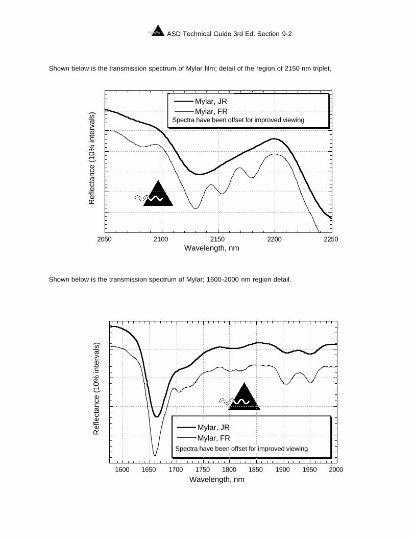
Shown below is the transmission spectrum of Mylar film; detail of the region of 2150 nm triplet. Shown below is the transmission spectrum of Mylar; 1600-2000 nm region detail.
2050 2100 2150 2200 2250
Mylar, JRMylar, FR
Ref
lect
ance
(10%
inte
rval
s)
Wavelength, nm
Spectra have been offset for improved viewing
1600 1650 1700 1750 1800 1850 1900 1950 2000
Mylar, JRMylar, FR
Ref
lect
ance
(10%
inte
rval
s)
Wavelength, nm
Spectra have been offset for improved viewing
ASD Technical Guide 3rd Ed. Section 9-3
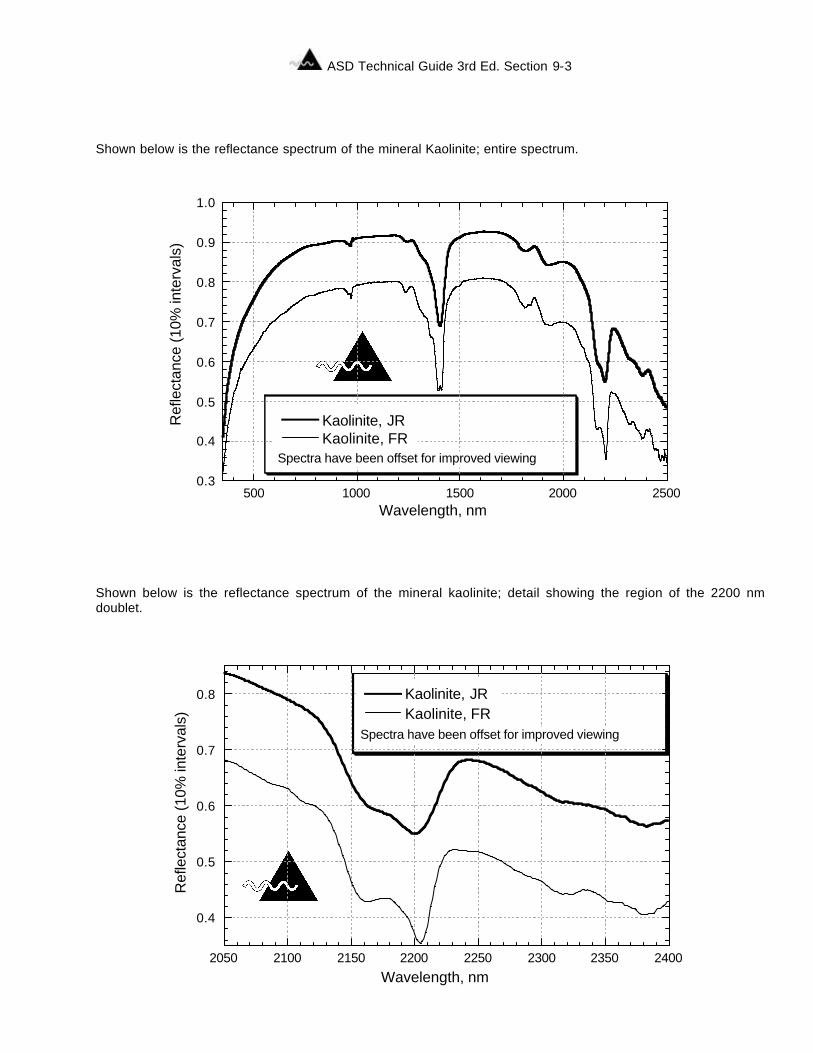
Shown below is the reflectance spectrum of the mineral Kaolinite; entire spectrum. Shown below is the reflectance spectrum of the mineral kaolinite; detail showing the region of the 2200 nm doublet.
500 1000 1500 2000 2500
Kaolinite, JRKaolinite, FR
0.3
0.4
0.5
0.6
0.7
0.8
0.9
1.0
Ref
lect
ance
(10%
inte
rval
s)
Wavelength, nm
Spectra have been offset for improved viewing
2050 2100 2150 2200 2250 2300 2350 2400
Kaolinite, JRKaolinite, FR
0.4
0.5
0.6
0.7
0.8
Ref
lect
ance
(10%
inte
rval
s)
Wavelength, nm
Spectra have been offset for improved viewing
ASD Technical Guide 3rd Ed. Section 9-4
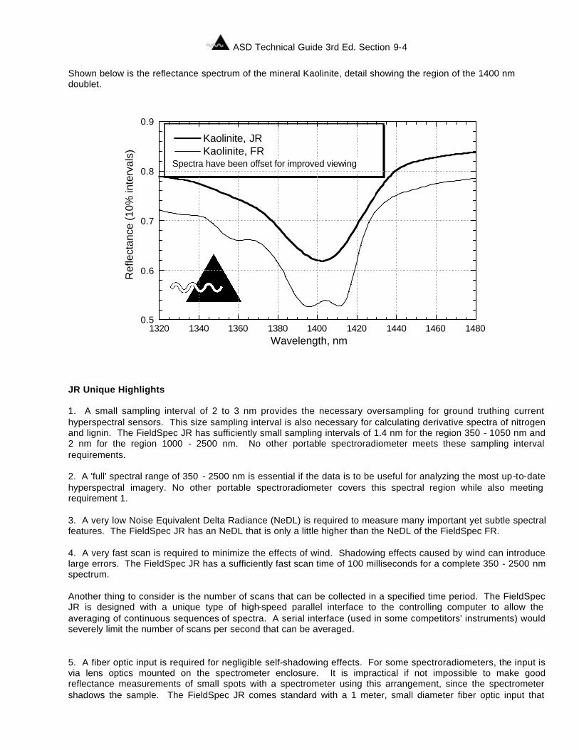
Shown below is the reflectance spectrum of the mineral Kaolinite, detail showing the region of the 1400 nm doublet.
JR Unique Highlights 1. A small sampling interval of 2 to 3 nm provides the necessary oversampling for ground truthing current hyperspectral sensors. This size sampling interval is also necessary for calculating derivative spectra of nitrogen and lignin. The FieldSpec JR has sufficiently small sampling intervals of 1.4 nm for the region 350 - 1050 nm and 2 nm for the region 1000 - 2500 nm. No other portable spectroradiometer meets these sampling interval requirements. 2. A 'full' spectral range of 350 - 2500 nm is essential if the data is to be useful for analyzing the most up-to-date hyperspectral imagery. No other portable spectroradiometer covers this spectral region while also meeting requirement 1. 3. A very low Noise Equivalent Delta Radiance (NeDL) is required to measure many important yet subtle spectral features. The FieldSpec JR has an NeDL that is only a little higher than the NeDL of the FieldSpec FR. 4. A very fast scan is required to minimize the effects of wind. Shadowing effects caused by wind can introduce large errors. The FieldSpec JR has a sufficiently fast scan time of 100 milliseconds for a complete 350 - 2500 nm spectrum. Another thing to consider is the number of scans that can be collected in a specified time period. The FieldSpec JR is designed with a unique type of high-speed parallel interface to the controlling computer to allow the averaging of continuous sequences of spectra. A serial interface (used in some competitors' instruments) would severely limit the number of scans per second that can be averaged.
5. A fiber optic input is required for negligible self-shadowing effects. For some spectroradiometers, the input is via lens optics mounted on the spectrometer enclosure. It is impractical if not impossible to make good reflectance measurements of small spots with a spectrometer using this arrangement, since the spectrometer shadows the sample. The FieldSpec JR comes standard with a 1 meter, small diameter fiber optic input that
1320 1340 1360 1380 1400 1420 1440 1460 1480
Kaolinite, JRKaolinite, FR
0.5
0.6
0.7
0.8
0.9R
efle
ctan
ce (1
0% in
terv
als)
Wavelength, nm
Spectra have been offset for improved viewing
ASD Technical Guide 3rd Ed. Section 9-5
carries signal directly into the spectrometer (signal carried directly into the spectrometer avoids large signal losses associated with detachable / coupled fiber optic options that other manufactures may offer). 6. Many in-situ field applications require a broad field-of-view, for example, for a spot size that closely matches the hyperspectral image pixels. Other examples include collecting data of large area backgrounds as well as other large area targets. The standard built-in fiberoptic input of the FieldSpec JR has the largest field-of-view of any portable spectroradiometer (25 degrees full conical angle). Optional narrower field-of-view attachable foreoptics are also available at additional cost. 7. When designing the FieldSpec JR spectrometer, we paid particular attention to the potential problem of scattered light. Careful baffling of the incoming light and special light traps for the zero-order light from the grating have been implemented. All interior surfaces are painted with ultra-low reflectance coatings. The detectors are covered with order separation filters. These filters reject not only second-order-diffracted light but also cut out other stray scattered light reaching the detector elements. The holographic gratings and extensive baffling used in the FieldSpec JR spectrometers also significantly reduce scattered light noise. The stray light level within the FieldSpec JR spectrometers is less than 0.02%. 8. The FieldSpec JR incorporates a unique combination of hardware and software known as Driftlock ('Driftlock' is a trademark of ASD). Driftlock automatically updates dark-current for every measurement from masked pixels in the silicon array. 9. Many in-situ field measurements require a portable instrument that is lightweight and carried in a way that allows fast measurements while moving from target to target. The FieldSpec can actually be worn around the waist for easy walk-along, spot-to-spot measurements. 10. The FieldSpec JR is fully upgradable to a FieldSpec FR at additional cost. FieldSpec NIR JR (1000 - 2500 nm) ASD has developed a JR, a lower cost alternative to our NIR version of the FieldSpec. The use of lower performance detectors and optics allow ASD to price the FieldSpec NIR JR significantly lower that ASD’s existing FieldSpec NIR instrument. The FieldSpec NIR JR spectroradiometer is fully upgradeable to the FieldSpec NIR spectroradiometer (at additional cost). The FieldSpec NIR JR spectroradiometer has the same look and feel as the FieldSpec NIR but has poorer spectral resolution and noise equivalent radiance. Please review the 1000 - 2500 nm region of the FieldSpec JR specifications above for equivalent NIR JR specifications.

ASD Technical Guide 3rd Ed. Section 9-6
ASD Technical Guide 3rd Ed. Section 10-1
Section 10 FieldSpec UV/VNIR (350 -1050 nm) The FieldSpec UV/VNIR looks the same as a FieldSpec FR. The primary differences are in spectral range total weight and user interface settings. The UV/VNIR (or as we call it here at ASD,'VNIR') has user selectable integration times, rather than the fixed scan time and auto optimization software of the FR. Several important features of the FieldSpec UV/VNIR make it the best and unique choice for a field portable spectroradiometer: The FieldSpec UV/VNIR is a post dispersive spectrometer. The FieldSpec UV/VNIR spectroradiometer uses a direct path fiber optic input. The FieldSpec UV/VNIR spectroradiometer has an unbeatable combination of speed and sensitivity. The FieldSpec UV/VNIR spectroradiometer has the nominal spectral range of 350 - 1050 nm for analyzing many current hyperspectral images, while maintaining optimal: spectral resolution, signal-to-noise. The FieldSpec UV/VNIR has excellent stray light rejection. The FieldSpec UV/VNIR features the unique Driftlock™ dark-drift correction system. The FieldSpec UV/VNIR has the largest standard field-of-view of any portable spectroradiometer. The FieldSpec UV/VNIR spectroradiometer is very lightweight, small and 'wear-able'. The FieldSpec UV/VNIR spectroradiometer has the ability to be upgraded to a dual spectrometer system. The FieldSpec UV/VNIR spectroradiometer has the ability to be upgraded to a FieldSpec FR. VNIR Post Dispersive Spectrometer All ASD spectrometers are “post-dispersive”. Because portable spectrometers are typically used outside the controlled laboratory environment, they are exposed to much higher levels of ambient light. In almost all cases, some of this ambient light will stray into the sample being measured. The errors produced by this ambient stray light are much greater for a pre-dispersive spectrometer than they are for a spectrometer that is post-dispersive. In a pre-dispersive spectrometer, the sample is illuminated with monochromatic light. Light scattered off or transmitted through the sample is then collected and delivered to the instrument’s detector. Ambient light that strays into the sample being measured is also collected. Thus, both the monochromatic illumination from the instrument and all wavelengths of the ambient stray light are delivered to the detector. Because the stray ambient light signal can represent a large fraction of the total light signal measured by the detector, it is a major source of error. While this source or error can be minimized by completely shielding the sample form all sources of ambient illumination, this often precludes the use of most reflectance and transmittance fiber optic probes. In a post-dispersive spectrometer, the sample is illuminated with white light. Light scattered off or transmitted through the sample is then dispersed and delivered to the entrance slit of the instrument’s spectrometer. As with the pre-dispersive spectrometer, ambient light that strays into the sample being measured is also collected. The difference is that in the post-dispersive instrument, only ambient stray light of the same wavelength as that being measured by the detector is added to the signal resulting from the instrument’s illumination of the sample. Thus, the stray ambient light signal represents a small fraction of the total light signal measured by the detector. VNIR Direct Path Fiberoptic Input The FieldSpecUV/VNIR spectroradiometer uses a 1.5 meter fiber optic input that feeds directly into the spectrometer. There are two advantages to this arrangement. First, the fiber optic input allows the user to quickly move and aim the very lightweight fiber optic probe from point to point without having to move the entire spectroradiometer. Secondly, since the fiber optic is connected directly into the spectroradiometer there is none of the signal losses otherwise associated with detachable couplings (detachable couplings typically result in as high as 50% signal loss).
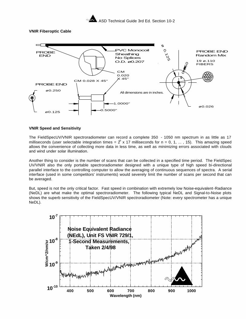
ASD Technical Guide 3rd Ed. Section 10-2
VNIR Fiberoptic Cable
VNIR Speed and Sensitivity The FieldSpecUV/VNIR spectroradiometer can record a complete 350 - 1050 nm spectrum in as little as 17 milliseconds (user selectable integration times = 2n x 17 milliseconds for n = 0, 1, ... , 15). This amazing speed allows the convenience of collecting more data in less time, as well as minimizing errors associated with clouds and wind under solar illumination. Another thing to consider is the number of scans that can be collected in a specified time period. The FieldSpec UV/VNIR also the only portable spectroradiometer designed with a unique type of high speed bi-directional parallel interface to the controlling computer to allow the averaging of continuous sequences of spectra. A serial interface (used in some competitors' instruments) would severely limit the number of scans per second that can be averaged. But, speed is not the only critical factor. Fast speed in combination with extremely low Noise-equivalent-Radiance (NeDL) are what make the optimal spectroradiometer. The following typical NeDL and Signal-to-Noise plots shows the superb sensitivity of the FieldSpecUV/VNIR spectroradiometer (Note: every spectrometer has a unique NeDL). 10-10
10-9
10-8
10-7
400 500 600 700 800 900 1000
Noise Equivalent Radiance(NEdL), Unit FS VNIR 729/1,1-Second Measurements,
Taken 2/4/98
W/c
m^2
/nm
/sr
Wavelength (nm)
CM 0.028 X 45°
PVC Monocoil SheathingNo Splices O.D. ø 0.207
ø 0.250
ø 0.125
ENDPROBE
PROBE END
CM 0.020 X 45°
1.0000"
0.5000"
ø0
.25
0
ø0.1
25
Random MixPROBE END
19 ø .110 FIBERS
ø 0.026
All dimensions are in inches.
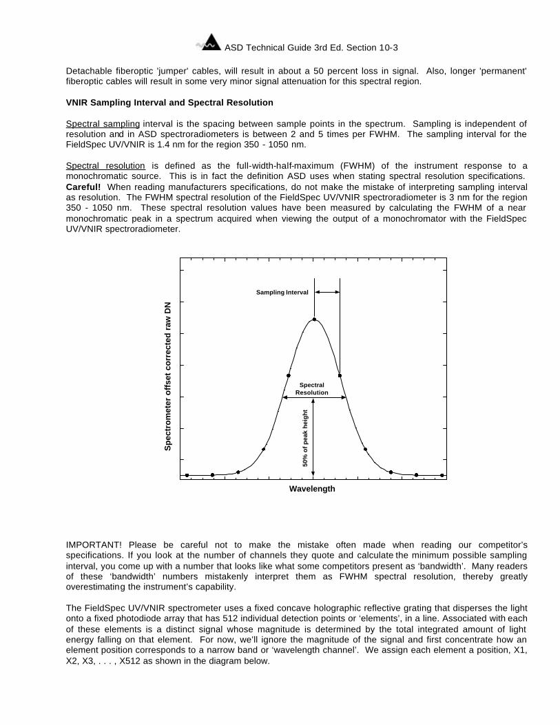
ASD Technical Guide 3rd Ed. Section 10-3
Detachable fiberoptic 'jumper' cables, will result in about a 50 percent loss in signal. Also, longer 'permanent' fiberoptic cables will result in some very minor signal attenuation for this spectral region. VNIR Sampling Interval and Spectral Resolution Spectral sampling interval is the spacing between sample points in the spectrum. Sampling is independent of resolution and in ASD spectroradiometers is between 2 and 5 times per FWHM. The sampling interval for the FieldSpec UV/VNIR is 1.4 nm for the region 350 - 1050 nm. Spectral resolution is defined as the full-width-half-maximum (FWHM) of the instrument response to a monochromatic source. This is in fact the definition ASD uses when stating spectral resolution specifications. Careful! When reading manufacturers specifications, do not make the mistake of interpreting sampling interval as resolution. The FWHM spectral resolution of the FieldSpec UV/VNIR spectroradiometer is 3 nm for the region 350 - 1050 nm. These spectral resolution values have been measured by calculating the FWHM of a near monochromatic peak in a spectrum acquired when viewing the output of a monochromator with the FieldSpec UV/VNIR spectroradiometer. IMPORTANT! Please be careful not to make the mistake often made when reading our competitor’s specifications. If you look at the number of channels they quote and calculate the minimum possible sampling interval, you come up with a number that looks like what some competitors present as ‘bandwidth’. Many readers of these ‘bandwidth’ numbers mistakenly interpret them as FWHM spectral resolution, thereby greatly overestimating the instrument’s capability. The FieldSpec UV/VNIR spectrometer uses a fixed concave holographic reflective grating that disperses the light onto a fixed photodiode array that has 512 individual detection points or ‘elements’, in a line. Associated with each of these elements is a distinct signal whose magnitude is determined by the total integrated amount of light energy falling on that element. For now, we’ll ignore the magnitude of the signal and first concentrate how an element position corresponds to a narrow band or ‘wavelength channel’. We assign each element a position, X1, X2, X3, . . . , X512 as shown in the diagram below.
Wavelength
Sampling Interval
SpectralResolution
50%
of
pea
k h
eig
ht
Spe
ctro
met
er o
ffse
t co
rrec
ted
raw
DN
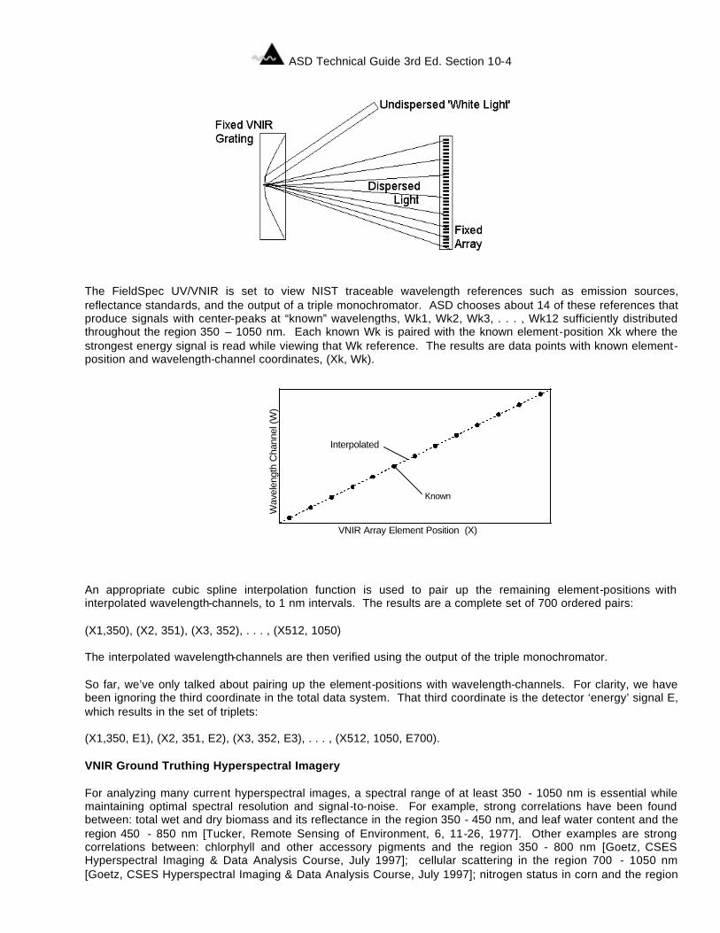
ASD Technical Guide 3rd Ed. Section 10-4
The FieldSpec UV/VNIR is set to view NIST traceable wavelength references such as emission sources, reflectance standards, and the output of a triple monochromator. ASD chooses about 14 of these references that produce signals with center-peaks at “known” wavelengths, Wk1, Wk2, Wk3, . . . , Wk12 sufficiently distributed throughout the region 350 – 1050 nm. Each known Wk is paired with the known element-position Xk where the strongest energy signal is read while viewing that Wk reference. The results are data points with known element-position and wavelength-channel coordinates, (Xk, Wk). An appropriate cubic spline interpolation function is used to pair up the remaining element-positions with interpolated wavelength-channels, to 1 nm intervals. The results are a complete set of 700 ordered pairs: (X1,350), (X2, 351), (X3, 352), . . . , (X512, 1050) The interpolated wavelength-channels are then verified using the output of the triple monochromator. So far, we’ve only talked about pairing up the element-positions with wavelength-channels. For clarity, we have been ignoring the third coordinate in the total data system. That third coordinate is the detector ‘energy’ signal E, which results in the set of triplets: (X1,350, E1), (X2, 351, E2), (X3, 352, E3), . . . , (X512, 1050, E700). VNIR Ground Truthing Hyperspectral Imagery For analyzing many current hyperspectral images, a spectral range of at least 350 - 1050 nm is essential while maintaining optimal spectral resolution and signal-to-noise. For example, strong correlations have been found between: total wet and dry biomass and its reflectance in the region 350 - 450 nm, and leaf water content and the region 450 - 850 nm [Tucker, Remote Sensing of Environment, 6, 11-26, 1977]. Other examples are strong correlations between: chlorphyll and other accessory pigments and the region 350 - 800 nm [Goetz, CSES Hyperspectral Imaging & Data Analysis Course, July 1997]; cellular scattering in the region 700 - 1050 nm [Goetz, CSES Hyperspectral Imaging & Data Analysis Course, July 1997]; nitrogen status in corn and the region
Wav
elen
gth
Cha
nnel
(W)
VNIR Array Element Position (X)
Interpolated
Known
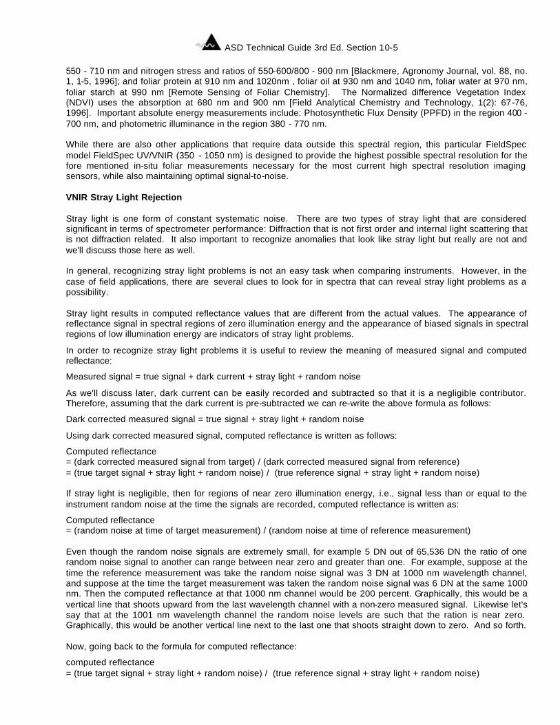
ASD Technical Guide 3rd Ed. Section 10-5
550 - 710 nm and nitrogen stress and ratios of 550-600/800 - 900 nm [Blackmere, Agronomy Journal, vol. 88, no. 1, 1-5, 1996]; and foliar protein at 910 nm and 1020nm , foliar oil at 930 nm and 1040 nm, foliar water at 970 nm, foliar starch at 990 nm [Remote Sensing of Foliar Chemistry]. The Normalized difference Vegetation Index (NDVI) uses the absorption at 680 nm and 900 nm [Field Analytical Chemistry and Technology, 1(2): 67-76, 1996]. Important absolute energy measurements include: Photosynthetic Flux Density (PPFD) in the region 400 - 700 nm, and photometric illuminance in the region 380 - 770 nm. While there are also other applications that require data outside this spectral region, this particular FieldSpec model FieldSpec UV/VNIR (350 - 1050 nm) is designed to provide the highest possible spectral resolution for the fore mentioned in-situ foliar measurements necessary for the most current high spectral resolution imaging sensors, while also maintaining optimal signal-to-noise. VNIR Stray Light Rejection Stray light is one form of constant systematic noise. There are two types of stray light that are considered significant in terms of spectrometer performance: Diffraction that is not first order and internal light scattering that is not diffraction related. It also important to recognize anomalies that look like stray light but really are not and we'll discuss those here as well. In general, recognizing stray light problems is not an easy task when comparing instruments. However, in the case of field applications, there are several clues to look for in spectra that can reveal stray light problems as a possibility. Stray light results in computed reflectance values that are different from the actual values. The appearance of reflectance signal in spectral regions of zero illumination energy and the appearance of biased signals in spectral regions of low illumination energy are indicators of stray light problems.
In order to recognize stray light problems it is useful to review the meaning of measured signal and computed reflectance:
Measured signal = true signal + dark current + stray light + random noise
As we'll discuss later, dark current can be easily recorded and subtracted so that it is a negligible contributor. Therefore, assuming that the dark current is pre-subtracted we can re-write the above formula as follows:
Dark corrected measured signal = true signal + stray light + random noise
Using dark corrected measured signal, computed reflectance is written as follows:
Computed reflectance = (dark corrected measured signal from target) / (dark corrected measured signal from reference) = (true target signal + stray light + random noise) / (true reference signal + stray light + random noise) If stray light is negligible, then for regions of near zero illumination energy, i.e., signal less than or equal to the instrument random noise at the time the signals are recorded, computed reflectance is written as:
Computed reflectance = (random noise at time of target measurement) / (random noise at time of reference measurement) Even though the random noise signals are extremely small, for example 5 DN out of 65,536 DN the ratio of one random noise signal to another can range between near zero and greater than one. For example, suppose at the time the reference measurement was take the random noise signal was 3 DN at 1000 nm wavelength channel, and suppose at the time the target measurement was taken the random noise signal was 6 DN at the same 1000 nm. Then the computed reflectance at that 1000 nm channel would be 200 percent. Graphically, this would be a vertical line that shoots upward from the last wavelength channel with a non-zero measured signal. Likewise let's say that at the 1001 nm wavelength channel the random noise levels are such that the ration is near zero. Graphically, this would be another vertical line next to the last one that shoots straight down to zero. And so forth. Now, going back to the formula for computed reflectance:
computed reflectance = (true target signal + stray light + random noise) / (true reference signal + stray light + random noise)
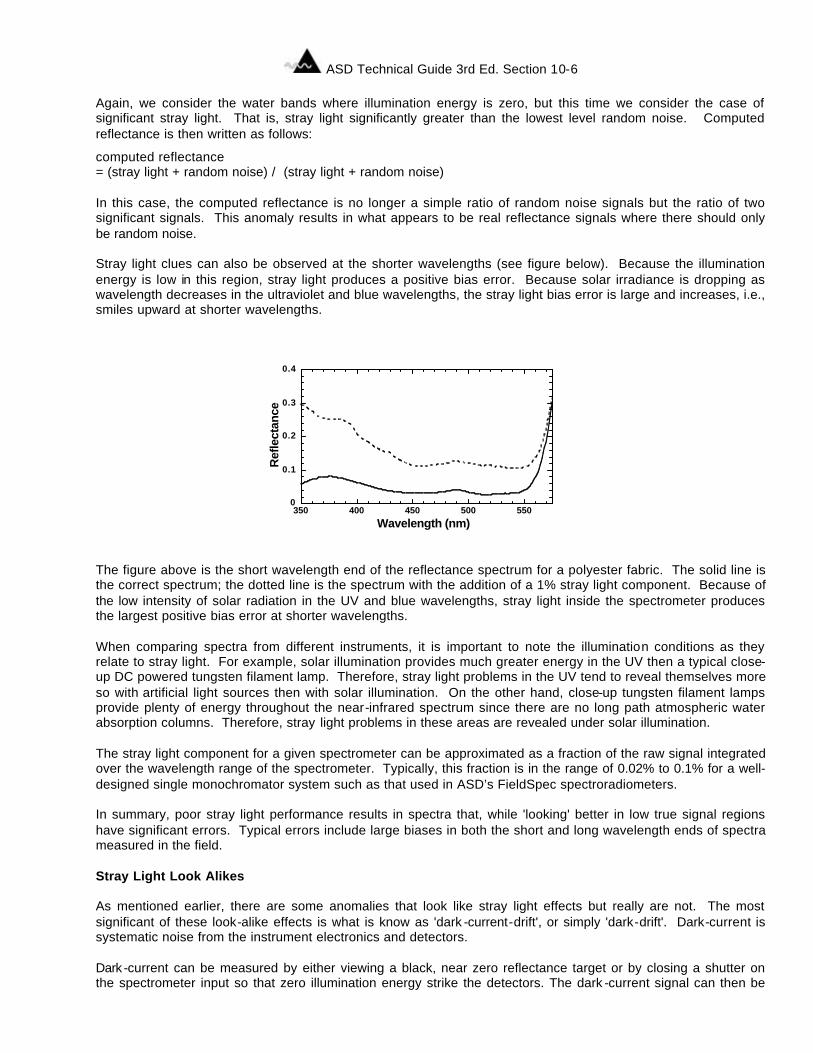
ASD Technical Guide 3rd Ed. Section 10-6
Again, we consider the water bands where illumination energy is zero, but this time we consider the case of significant stray light. That is, stray light significantly greater than the lowest level random noise. Computed reflectance is then written as follows:
computed reflectance = (stray light + random noise) / (stray light + random noise) In this case, the computed reflectance is no longer a simple ratio of random noise signals but the ratio of two significant signals. This anomaly results in what appears to be real reflectance signals where there should only be random noise. Stray light clues can also be observed at the shorter wavelengths (see figure below). Because the illumination energy is low in this region, stray light produces a positive bias error. Because solar irradiance is dropping as wavelength decreases in the ultraviolet and blue wavelengths, the stray light bias error is large and increases, i.e., smiles upward at shorter wavelengths. The figure above is the short wavelength end of the reflectance spectrum for a polyester fabric. The solid line is the correct spectrum; the dotted line is the spectrum with the addition of a 1% stray light component. Because of the low intensity of solar radiation in the UV and blue wavelengths, stray light inside the spectrometer produces the largest positive bias error at shorter wavelengths. When comparing spectra from different instruments, it is important to note the illumination conditions as they relate to stray light. For example, solar illumination provides much greater energy in the UV then a typical close-up DC powered tungsten filament lamp. Therefore, stray light problems in the UV tend to reveal themselves more so with artificial light sources then with solar illumination. On the other hand, close-up tungsten filament lamps provide plenty of energy throughout the near-infrared spectrum since there are no long path atmospheric water absorption columns. Therefore, stray light problems in these areas are revealed under solar illumination. The stray light component for a given spectrometer can be approximated as a fraction of the raw signal integrated over the wavelength range of the spectrometer. Typically, this fraction is in the range of 0.02% to 0.1% for a well-designed single monochromator system such as that used in ASD’s FieldSpec spectroradiometers. In summary, poor stray light performance results in spectra that, while 'looking' better in low true signal regions have significant errors. Typical errors include large biases in both the short and long wavelength ends of spectra measured in the field. Stray Light Look Alikes As mentioned earlier, there are some anomalies that look like stray light effects but really are not. The most significant of these look-alike effects is what is know as 'dark -current-drift', or simply 'dark-drift'. Dark-current is systematic noise from the instrument electronics and detectors. Dark -current can be measured by either viewing a black, near zero reflectance target or by closing a shutter on the spectrometer input so that zero illumination energy strike the detectors. The dark -current signal can then be
0
0.1
0.2
0.3
0.4
350 400 450 500 550
Ref
lect
ance
Wavelength (nm)
ASD Technical Guide 3rd Ed. Section 10-7
stored and subtracted from all subsequent measurements. The FieldSpec spectroradiometer includes mechanically controlled shutters and software for recording and automatically subtracting dark-current. Within short time periods, dark-current is relatively constant. However, during the initial start-up the spectrometer goes through a period where the internal components and external ambient temperature attempt to reach thermal equilibrium. During this period, the dark-current changes slowly as the change in temperature effects the efficiency of the internal components. These effects are most significant at the outer boundaries of the detectors' quantum efficiencies, i.e. at the low and high spectral regions of a given detector. Even after thermal equilibrium is reached, less significant dark-drift can occur with fluctuations in external ambient temperature. Dark -drift can be minimized by updatng the dark-current frequently during the first 15 minutes of operation, and then less frequently after the system has reached thermal equilibrium. The frequency for dark-current updating after thermal equilibrium should be based on the stability of the ambient conditions and the priority of the regions most effected by dark-drift. As previously mentioned, dark -drift is most noticeable in the regions of least quantum efficiency. For example, in the lower UV regions of a silicon detector. If dark current is not updated, such drift looks very similar to the upward smiling effect that can also be caused by stray light. The difference is that a dark-drift smile forms gradually over time when dark current is not updated, while stray light effects are constant. Another example of dark-drift can be recognized by a smile-down at the upper most NIR regions of the silicon detector. If stray light is negligible, these dark -drift effects can be easily dealt with by simply updating dark-current more frequently. VNIR Driftlock In addition to these methods of dealing with dark-drift, the more the FieldSpec VNIR incorporate a unique combination of hardware and software known as Driftlock ('Driftlock' is a trademark of ASD). Driftlock automatically updates dark-current for every measurement from masked pixels in the silicon array. VNIR Large Field-of-View Many in-situ field applications require a broad field-of-view, for example, for a spot size that closely matches the hyperspectral image pixels. Other examples include collecting data of large area backgrounds as well as other large area targets. The standard built-in fiberoptic input of the FieldSpec has the largest field-of-view of any portable spectroradiometer (25 degrees full conical angle). Optional narrower field-of-view attachable foreoptics are also available at additional cost. For more details see page 7-3. VNIR Light Weight, Small, and Wear-able In-situ measurements or measurements made from a light payload elevation device, such as a balloon, require a portable instrument that is light-weight and carried in a way that allows fast measurements while moving from spot to spot or elevation to elevation. The FieldSpec UV/VNIR can actually be worn around the waist for easy walk-along, spot-to-spot measurements and has the lightest payload weight for a spectrometer of its performance specifications. VNIR Upgrade to Dual Spectrometer System The FieldSpec UV/VNIR spectroradiometer has the ability to be upgraded to a dual spectrometer system (see price list for upgrade cost). For many foliar and oceanographic applications, a dual spectrometer system is greatly prefered to a single spectrometer system. Particularly under conditions of rapidly changing illumination, e.g., on a day with partly cloudy skies, it is essential to simultaneously measure downwelling irradiance in conjunction with the upwelling radiance reflected from the target. VNIR Upgrade to a FieldSpec FR There are many applications that require measurements beyond the spectral range of the FieldSpec UV/VNIR (350 - 1050 nm). Accordingly, ASD offers an option at additional cost for upgrading the FieldSpec UV/VNIR to a FieldSpec FR (350 - 2500 nm).
ASD Technical Guide 3rd Ed. Section 10-8
FieldSpec Dual UV/VNIR (350 -1050 nm) The FieldSpec Dual UV/VNIR looks the same as the standard 'single-beam' FieldSpec UV/VNIR. The primary differences are in total weight and user interface settings. In addition to all the unique benefits of the 'single-beam' FieldSpec UV/VNIR the FieldSpec Dual UV/VNIR is the only portable spectroradiometer that can measure two separate light components simultaneously. For many applications, a 'dual-beam' system is necessary instead of a single 'single-beam' system. Particularly under conditions of changing illumination (e.g. on a day with partly cloudy skies), it is essential to simultaneously measure downwelling irradiance in conjunction with the measurement of upwelling reflected radiance. FieldSpec UV/VNIR/CCD The FieldSpec UV/VNIR/CCD looks the same as the standard FieldSpec UV/VNIR. The primary differences are the detectors and the illumination conditions under which each are considered optimal. The FieldSpec UV/VNIR/CCD uses Charge-Coupled Device (CCD) array while the standard FieldSpec UV/VNIR uses a Photo-diode array (PDA). A CCD is a two dimensional silicon array of detectors manufactured into a single chip and gated for sequential transfer and reading of pixels. A Photodiode Array (PDA) is a one demensional silicon array of detectors manufactued into a single chip. For a CCD, a whole column of pixels at a specific wavelength are co-added or "binned" in a summing register and read as a single pixel. The sensitivity of a CCD is superior to a photo diode array (PDA), but its dynamic range is lower. This type of detector is ideally suited for low light level applications. These include: in situ measurements of apparent optical properties of lake and sea water, fluorescence, and bioluminescence. In general, the S/N of a CCD is superior to a PDA only at VERY LOW LIGHT LEVELS. However, for normal to high light levels the S/N of a CCD is not as good as that of a PDA. The CCD is best used for things like fluorescence, bioluminescence, and solar energy measurements under DEEP, dark natural waters. The PDA is best used for surface measurements under solar illumination and solar energy measurements under shallow, clear natural waters. While the S/N of a PDA is not as good as a CCD at VERY low light levels, the PDA CAN measure very low light levels by setting a long integration time. So, if your mission is to purchase an instrument for a variety of applications, the PDA is probably your best bet. The CCD should be considered only if you wish to specialize in VERY low light level measurements. The plot below shows and example NeDL for the standard 64 element high CCD model.
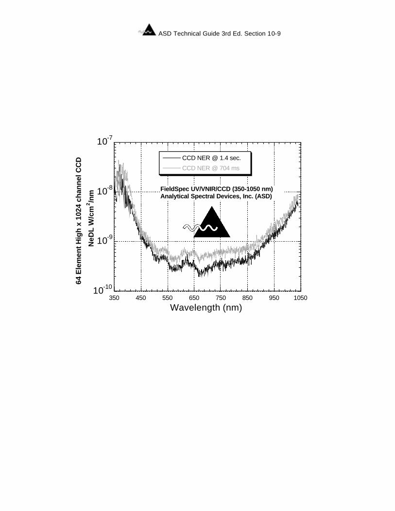
ASD Technical Guide 3rd Ed. Section 10-9
10-10
10-9
10-8
10-7
350 450 550 650 750 850 950 1050
CCD NER @ 1.4 sec.
CCD NER @ 704 ms
64 E
lem
ent H
igh
x 10
24 c
hann
el C
CD
NeD
L W
/cm
2 /nm
Wavelength (nm)
FieldSpec UV/VNIR/CCD (350-1050 nm)Analytical Spectral Devices, Inc. (ASD)

ASD Technical Guide 3rd Ed. Section 10-10
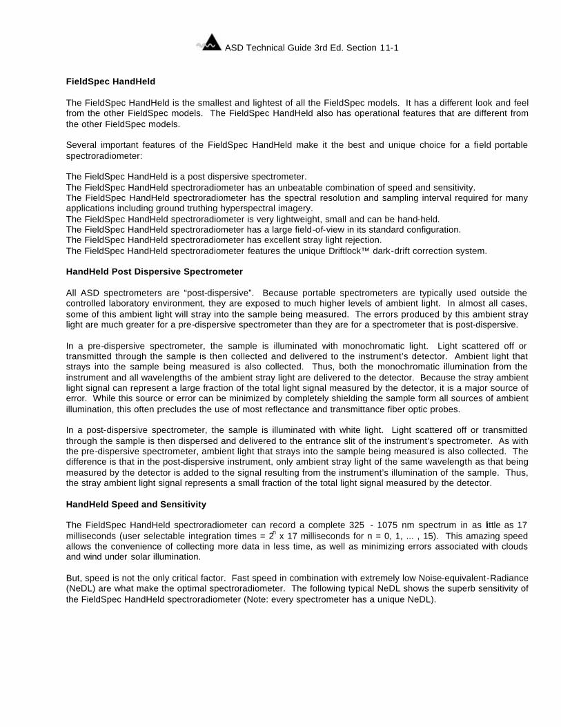
ASD Technical Guide 3rd Ed. Section 11-1
Section 11 FieldSpec HandHeld The FieldSpec HandHeld is the smallest and lightest of all the FieldSpec models. It has a different look and feel from the other FieldSpec models. The FieldSpec HandHeld also has operational features that are different from the other FieldSpec models. Several important features of the FieldSpec HandHeld make it the best and unique choice for a field portable spectroradiometer: The FieldSpec HandHeld is a post dispersive spectrometer. The FieldSpec HandHeld spectroradiometer has an unbeatable combination of speed and sensitivity. The FieldSpec HandHeld spectroradiometer has the spectral resolution and sampling interval required for many applications including ground truthing hyperspectral imagery. The FieldSpec HandHeld spectroradiometer is very lightweight, small and can be hand-held. The FieldSpec HandHeld spectroradiometer has a large field-of-view in its standard configuration. The FieldSpec HandHeld spectroradiometer has excellent stray light rejection. The FieldSpec HandHeld spectroradiometer features the unique Driftlock™ dark-drift correction system. HandHeld Post Dispersive Spectrometer All ASD spectrometers are “post-dispersive”. Because portable spectrometers are typically used outside the controlled laboratory environment, they are exposed to much higher levels of ambient light. In almost all cases, some of this ambient light will stray into the sample being measured. The errors produced by this ambient stray light are much greater for a pre-dispersive spectrometer than they are for a spectrometer that is post-dispersive. In a pre-dispersive spectrometer, the sample is illuminated with monochromatic light. Light scattered off or transmitted through the sample is then collected and delivered to the instrument’s detector. Ambient light that strays into the sample being measured is also collected. Thus, both the monochromatic illumination from the instrument and all wavelengths of the ambient stray light are delivered to the detector. Because the stray ambient light signal can represent a large fraction of the total light signal measured by the detector, it is a major source of error. While this source or error can be minimized by completely shielding the sample form all sources of ambient illumination, this often precludes the use of most reflectance and transmittance fiber optic probes. In a post-dispersive spectrometer, the sample is illuminated with white light. Light scattered off or transmitted through the sample is then dispersed and delivered to the entrance slit of the instrument’s spectrometer. As with the pre-dispersive spectrometer, ambient light that strays into the sample being measured is also collected. The difference is that in the post-dispersive instrument, only ambient stray light of the same wavelength as that being measured by the detector is added to the signal resulting from the instrument’s illumination of the sample. Thus, the stray ambient light signal represents a small fraction of the total light signal measured by the detector. HandHeld Speed and Sensitivity The FieldSpec HandHeld spectroradiometer can record a complete 325 - 1075 nm spectrum in as little as 17 milliseconds (user selectable integration times = 2n x 17 milliseconds for n = 0, 1, ... , 15). This amazing speed allows the convenience of collecting more data in less time, as well as minimizing errors associated with clouds and wind under solar illumination. But, speed is not the only critical factor. Fast speed in combination with extremely low Noise-equivalent-Radiance (NeDL) are what make the optimal spectroradiometer. The following typical NeDL shows the superb sensitivity of the FieldSpec HandHeld spectroradiometer (Note: every spectrometer has a unique NeDL).
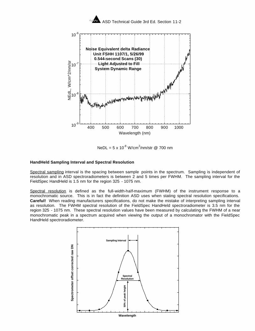
ASD Technical Guide 3rd Ed. Section 11-2
NeDL = 5 x 10⁻⁸ W/cm2/nm/str @ 700 nm
HandHeld Sampling Interval and Spectral Resolution Spectral sampling interval is the spacing between sample points in the spectrum. Sampling is independent of resolution and in ASD spectroradiometers is between 2 and 5 times per FWHM. The sampling interval for the FieldSpec HandHeld is 1.5 nm for the region 325 - 1075 nm. Spectral resolution is defined as the full-width-half-maximum (FWHM) of the instrument response to a monochromatic source. This is in fact the definition ASD uses when stating spectral resolution specifications. Careful! When reading manufacturers specifications, do not make the mistake of interpreting sampling interval as resolution. The FWHM spectral resolution of the FieldSpec HandHeld spectroradiometer is 3.5 nm for the region 325 - 1075 nm. These spectral resolution values have been measured by calculating the FWHM of a near monochromatic peak in a spectrum acquired when viewing the output of a monochromator with the FieldSpec HandHeld spectroradiometer.
Wavelength
Sampling Interval
SpectralResolution
50%
of
peak
hei
ght
Spe
ctro
met
er o
ffse
t co
rrec
ted
raw
DN
10-9
10-8
10-7
10-6
400 500 600 700 800 900 1000
Noise Equivalent delta RadianceUnit FSHH 1107/1, 5/26/990.544-second Scans (30)
Light Adjusted to FillSystem Dynamic Range
NE
dL, W
/cm
^2/n
m/s
r
Wavelength (nm)
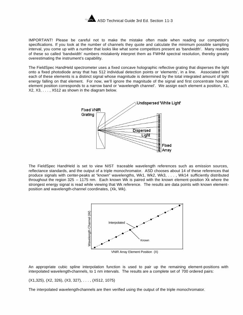
ASD Technical Guide 3rd Ed. Section 11-3
IMPORTANT! Please be careful not to make the mistake often made when reading our competitor’s specifications. If you look at the number of channels they quote and calculate the minimum possible sampling interval, you come up with a number that looks like what some competitors present as ‘bandwidth’. Many readers of these so called ‘bandwidth’ numbers mistakenly interpret them as FWHM spectral resolution, thereby greatly overestimating the instrument’s capability. The FieldSpec HandHeld spectrometer uses a fixed concave holographic reflective grating that disperses the light onto a fixed photodiode array that has 512 individual detection points or ‘elements’, in a line. Associated with each of these elements is a distinct signal whose magnitude is determined by the total integrated amount of light energy falling on that element. For now, we’ll ignore the magnitude of the signal and first concentrate how an element position corresponds to a narrow band or ‘wavelength channel’. We assign each element a position, X1, X2, X3, . . . , X512 as shown in the diagram below.
The FieldSpec HandHeld is set to view NIST traceable wavelength references such as emission sources, reflectance standards, and the output of a triple monochromator. ASD chooses about 14 of these references that produce signals with center-peaks at “known” wavelengths, Wk1, Wk2, Wk3, . . . , Wk14 sufficiently distributed throughout the region 325 – 1175 nm. Each known Wk is paired with the known element-position Xk where the strongest energy signal is read while viewing that Wk reference. The results are data points with known element-position and wavelength-channel coordinates, (Xk, Wk). An appropriate cubic spline interpolation function is used to pair up the remaining element-positions with interpolated wavelength-channels, to 1 nm intervals. The results are a complete set of 700 ordered pairs: (X1,325), (X2, 326), (X3, 327), . . . , (X512, 1075) The interpolated wavelength-channels are then verified using the output of the triple monochromator.
Wav
elen
gth
Cha
nnel
(W)
VNIR Array Element Position (X)
Interpolated
Known
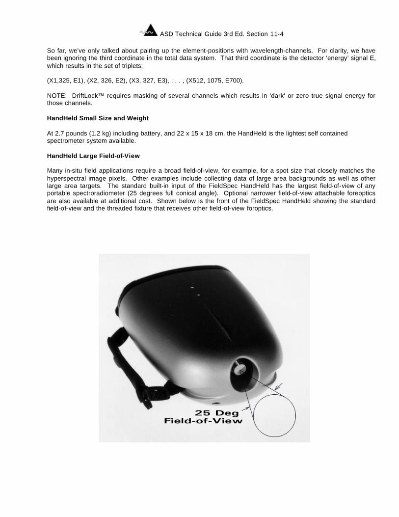
ASD Technical Guide 3rd Ed. Section 11-4
So far, we’ve only talked about pairing up the element-positions with wavelength-channels. For clarity, we have been ignoring the third coordinate in the total data system. That third coordinate is the detector ‘energy’ signal E, which results in the set of triplets: (X1,325, E1), (X2, 326, E2), (X3, 327, E3), . . . , (X512, 1075, E700). NOTE: DriftLock™ requires masking of several channels which results in 'dark' or zero true signal energy for those channels. HandHeld Small Size and Weight At 2.7 pounds (1.2 kg) including battery, and 22 x 15 x 18 cm, the HandHeld is the lightest self contained spectrometer system available. HandHeld Large Field-of-View Many in-situ field applications require a broad field-of-view, for example, for a spot size that closely matches the hyperspectral image pixels. Other examples include collecting data of large area backgrounds as well as other large area targets. The standard built-in input of the FieldSpec HandHeld has the largest field-of-view of any portable spectroradiometer (25 degrees full conical angle). Optional narrower field-of-view attachable foreoptics are also available at additional cost. Shown below is the front of the FieldSpec HandHeld showing the standard field-of-view and the threaded fixture that receives other field-of-view foroptics.
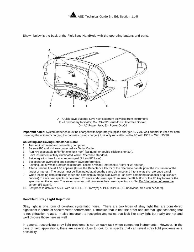
ASD Technical Guide 3rd Ed. Section 11-5
Shown below is the back of the FieldSpec HandHeld with the operating buttons and ports.
A – Quick-save Buttons: Save next spectrum delivered from instrument; B – Low Battery Indicator; C – RS-232 Serial-to-PC Interface Socket;
D – AC Power Jack; E – Power On/Off
Important notes: System batteries must be charged with separately supplied charger. 12V AC wall adaptor is used for both powering the unit and charging the batteries (using charger). Unit only runs attached to PC with DOS or Win95/98.
Collecting and Saving Reflectance Data: 1. Turn on instrument and controlling computer. 2. Be sure PC and HH are connected via Serial Cable. 3. Run HH executable (c:\hh\hh.exe [unit num] [cal num], or double-click on shortcut). 4. Point instrument at fully illuminated White Reference standard. 5. Set integration time for maximum signal (F1 and F2 keys). 6. Set spectrum averaging and spectrum save preferences. 7. Pointing unit at White Reference standard, collect a White Reference (F4 key or WR button). 8. After a uniform line at 1.00 appears (this is the Reflectance Factor of the reference panel), point the instrument at the
target of interest. The target must be illuminated at about the same distance and intensity as the reference panel. 9. When incoming data stabilizes (after one complete average is delivered) use save command (spacebar or quicksave
buttons) to save next spectrum delivered. To save and current spectrum, use the FR button or the F6 key to freeze the spectrum on the screen. The save command will now save the current spectrum to file. Don’t forget to unfreeze the screen (F6 again).
10. Postprocess data into ASCII with STABLE.EXE (arrays) or PORTSPEC.EXE (individual files with headers). HandHeld Stray Light Rejection Stray light is one form of constant systematic noise. There are two types of stray light that are considered significant in terms of spectrometer performance: Diffraction that is not first order and internal light scattering that is not diffraction related. It also important to recognize anomalies that look like stray light but really are not and we'll discuss those here as well. In general, recognizing stray light problems is not an easy task when comparing instruments. However, in the case of field applications, there are several clues to look for in spectra that can reveal stray light problems as a possibility.
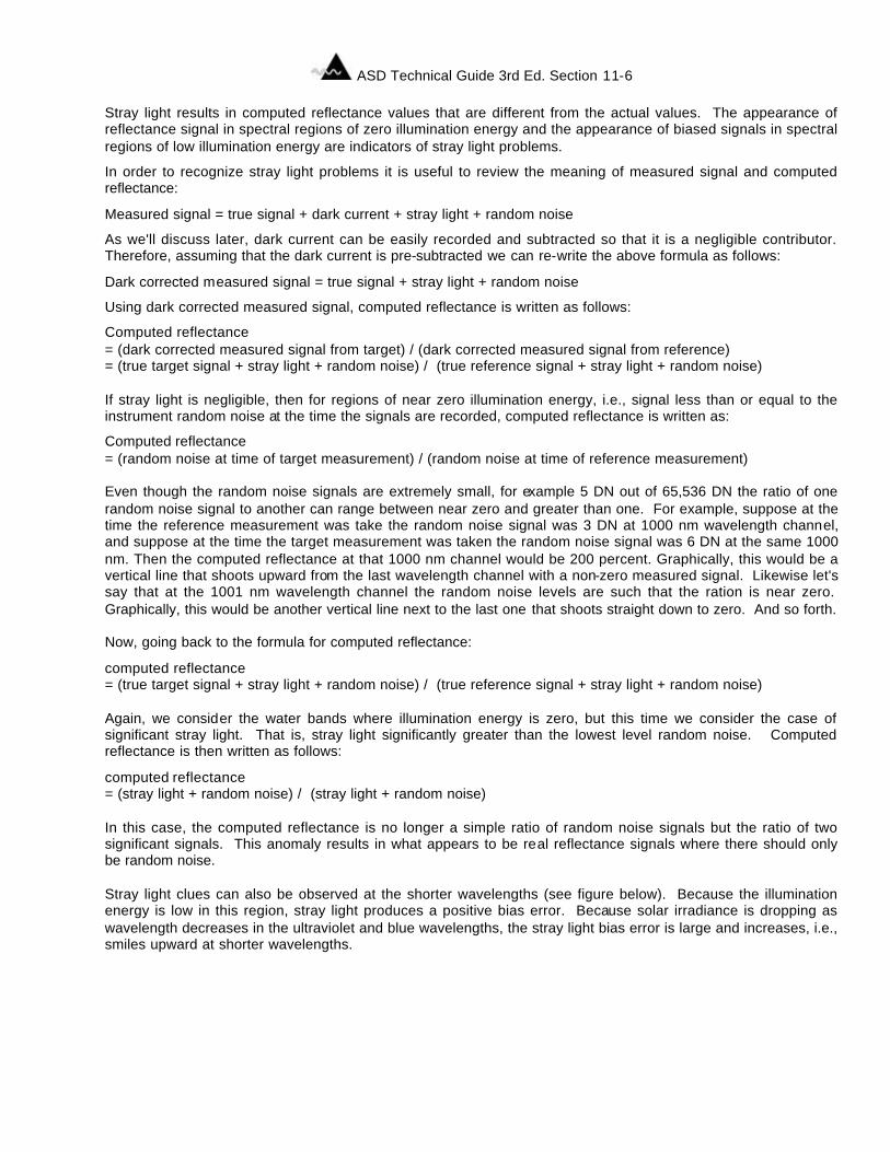
ASD Technical Guide 3rd Ed. Section 11-6
Stray light results in computed reflectance values that are different from the actual values. The appearance of reflectance signal in spectral regions of zero illumination energy and the appearance of biased signals in spectral regions of low illumination energy are indicators of stray light problems.
In order to recognize stray light problems it is useful to review the meaning of measured signal and computed reflectance:
Measured signal = true signal + dark current + stray light + random noise
As we'll discuss later, dark current can be easily recorded and subtracted so that it is a negligible contributor. Therefore, assuming that the dark current is pre-subtracted we can re-write the above formula as follows:
Dark corrected measured signal = true signal + stray light + random noise
Using dark corrected measured signal, computed reflectance is written as follows:
Computed reflectance = (dark corrected measured signal from target) / (dark corrected measured signal from reference) = (true target signal + stray light + random noise) / (true reference signal + stray light + random noise) If stray light is negligible, then for regions of near zero illumination energy, i.e., signal less than or equal to the instrument random noise at the time the signals are recorded, computed reflectance is written as:
Computed reflectance = (random noise at time of target measurement) / (random noise at time of reference measurement) Even though the random noise signals are extremely small, for example 5 DN out of 65,536 DN the ratio of one random noise signal to another can range between near zero and greater than one. For example, suppose at the time the reference measurement was take the random noise signal was 3 DN at 1000 nm wavelength channel, and suppose at the time the target measurement was taken the random noise signal was 6 DN at the same 1000 nm. Then the computed reflectance at that 1000 nm channel would be 200 percent. Graphically, this would be a vertical line that shoots upward from the last wavelength channel with a non-zero measured signal. Likewise let's say that at the 1001 nm wavelength channel the random noise levels are such that the ration is near zero. Graphically, this would be another vertical line next to the last one that shoots straight down to zero. And so forth. Now, going back to the formula for computed reflectance:
computed reflectance = (true target signal + stray light + random noise) / (true reference signal + stray light + random noise) Again, we consider the water bands where illumination energy is zero, but this time we consider the case of significant stray light. That is, stray light significantly greater than the lowest level random noise. Computed reflectance is then written as follows:
computed reflectance = (stray light + random noise) / (stray light + random noise) In this case, the computed reflectance is no longer a simple ratio of random noise signals but the ratio of two significant signals. This anomaly results in what appears to be real reflectance signals where there should only be random noise. Stray light clues can also be observed at the shorter wavelengths (see figure below). Because the illumination energy is low in this region, stray light produces a positive bias error. Because solar irradiance is dropping as wavelength decreases in the ultraviolet and blue wavelengths, the stray light bias error is large and increases, i.e., smiles upward at shorter wavelengths.
ASD Technical Guide 3rd Ed. Section 11-7
The figure above is the short wavelength end of the reflectance spectrum for a polyester fabric. The solid line is the correct spectrum; the dotted line is the spectrum with the addition of a 1% stray light component. Because of the low intensity of solar radiation in the UV and blue wavelengths, stray light inside the spectrometer produces the largest positive bias error at shorter wavelengths. When comparing spectra from different instruments, it is important to note the illumination conditions as they relate to stray light. For example, solar illumination provides much greater energy in the UV then a typical close-up DC powered tungsten filament lamp. Therefore, stray light problems in the UV tend to reveal themselves more so with artificial light sources then with solar illumination. On the other hand, close-up tungsten filament lamps provide plenty of energy throughout the near-infrared spectrum since there are no long path atmospheric water absorption columns. Therefore, stray light problems in these areas are revealed under solar illumination. The stray light component for a given spectrometer can be approximated as a fraction of the raw signal integrated over the wavelength range of the spectrometer. Typically, this fraction is in the range of 0.02% to 0.1% for a well-designed single monochromator system such as that used in ASD’s FieldSpec spectroradiometers. In summary, poor stray light performance results in spectra that, while 'looking' better in low true signal regions have significant errors. Typical errors include large biases in both the short and long wavelength ends of spectra measured in the field. Stray Light Look Alikes As mentioned earlier, there are some anomalies that look like stray light effects but really are not. The most significant of these look-alike effects is what is know as 'dark -current-drift', or simply 'dark-drift'. Dark-current is systematic noise from the instrument electronics and detectors. Dark -current can be measured by either viewing a black, near zero reflectance target or by closing a shutter on the spectrometer input so that zero illumination energy strike the detectors. The dark -current signal can then be stored and subtracted from all subsequent measurements. The FieldSpec spectroradiometer includes mechanically controlled shutters and soft ware for recording and automatically subtracting dark-current. Within short time periods, dark-current is relatively constant. However, during the initial start-up the spectrometer goes through a period where the internal components and external ambient temperature attempt to reach thermal equilibrium. During this period, the dark-current changes slowly as the change in temperature effects the efficiency of the internal components. These effects are most significant at the outer boundaries of the detectors' quantum efficiencies, i.e. at the low and high spectral regions of a given detector. Even after thermal equilibrium is reached, less significant dark-drift can occur with fluctuations in external ambient temperature. Dark -drift can be minimized by updatng the dark-current frequently during the first 15 minutes of operation, and then less frequently after the system has reached thermal equilibrium. The frequency for dark-current updating after thermal equilibrium should be based on the stability of the ambient conditions and the priority of the regions most effected by dark-drift. As previously mentioned, dark -drift is most noticeable in the regions of least quantum efficiency. For example, in the lower UV regions of a silicon detector. If dark current is not updated, such drift looks very similar to the
0
0.1
0.2
0.3
0.4
350 400 450 500 550
Ref
lect
ance
Wavelength (nm)
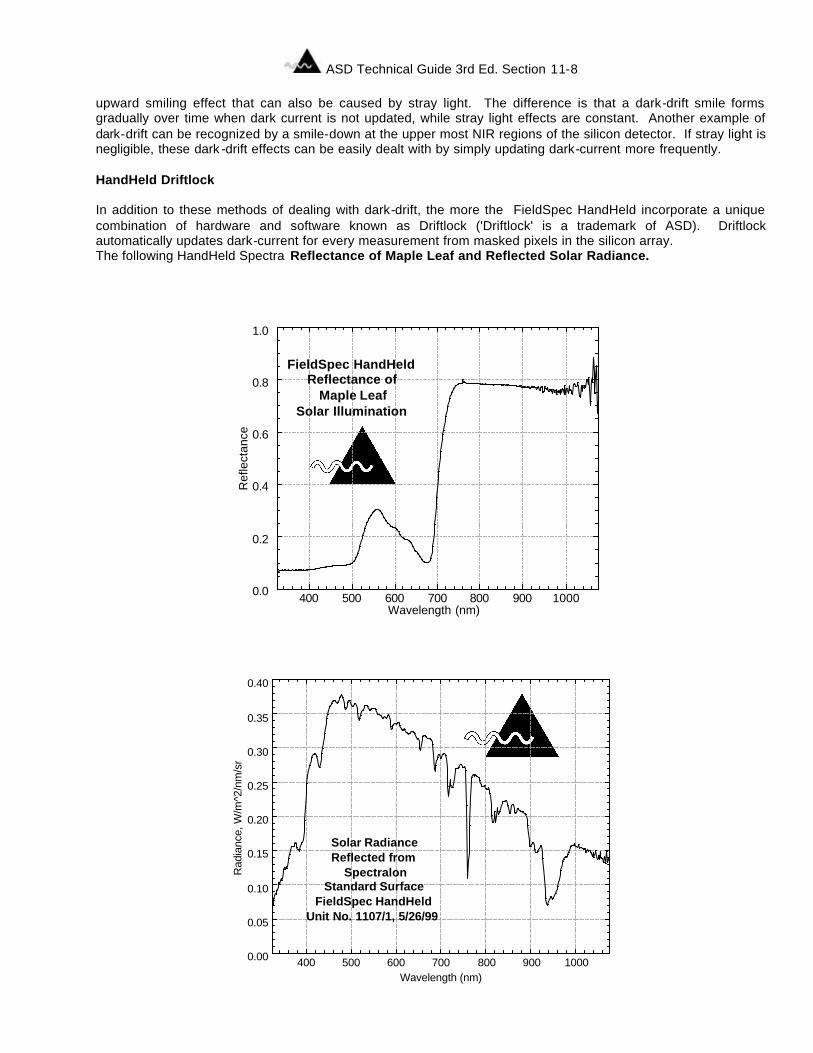
ASD Technical Guide 3rd Ed. Section 11-8
upward smiling effect that can also be caused by stray light. The difference is that a dark-drift smile forms gradually over time when dark current is not updated, while stray light effects are constant. Another example of dark-drift can be recognized by a smile-down at the upper most NIR regions of the silicon detector. If stray light is negligible, these dark -drift effects can be easily dealt with by simply updating dark-current more frequently. HandHeld Driftlock In addition to these methods of dealing with dark-drift, the more the FieldSpec HandHeld incorporate a unique combination of hardware and software known as Driftlock ('Driftlock' is a trademark of ASD). Driftlock automatically updates dark-current for every measurement from masked pixels in the silicon array. The following HandHeld Spectra Reflectance of Maple Leaf and Reflected Solar Radiance.
0.0
0.2
0.4
0.6
0.8
1.0
400 500 600 700 800 900 1000
Ref
lect
ance
Wavelength (nm)
FieldSpec HandHeldReflectance of
Maple LeafSolar Illumination
0.00
0.05
0.10
0.15
0.20
0.25
0.30
0.35
0.40
400 500 600 700 800 900 1000
Solar RadianceReflected from
SpectralonStandard Surface
FieldSpec HandHeldUnit No. 1107/1, 5/26/99
Rad
ianc
e, W
/m^2
/nm
/sr
Wavelength (nm)
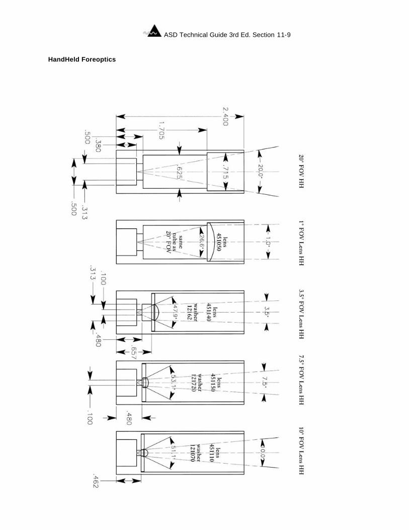
ASD Technical Guide 3rd Ed. Section 11-9
HandHeld Foreoptics

ASD Technical Guide 3rd Ed. Section 11-10

ASD Technical Guide 3rd Ed. Section 12-1
Section 12 LabSpec Pro Portable Spectrophotometer LabSpec Pro is the first, truly portable, near infrared analyzer that offers unprecedented ruggedness, durability and reliability in a laboratory instrument. Equipped with a built in handle and internal batteries, LabSpec Pro offers the flexibility to get out of the lab, collect samples, make demonstrations, prove concepts or trouble shoot problems. Its ultra tough case, made of the same material as industrial power tools, and chemically resistant aluminum front panel makes LabSpec Pro ideal for use in virtually any environment. LabSpec Pro has laboratory accuracy to meet your QA/QC measurement needs. A host of probes and sampling accessories are available for liquids, powders, and slurries. With a wavelength range of 350 nm – 2500 nm that can penetrate many plastic bags, bottles or glass vials, LabSpec Pro offers the convenience of testing samples in their original containers. With a super fast scanning time of 0.1 seconds and a sampling interval of 2 nm, LabSpec Pro is ideal for non-destructive quality control applications. Industries with NIR Applications: Chemical, Pharmaceutical, Petrochemical, Food & Beverage, Pulp & Paper, Textile, Paint, & Tobacco. LabSpec Pro Spectral Ranges Model Number 1000-1800 nm A108280 1000-2500 nm A108300 350-2500 nm A108310 LabSpec Pro Features & Advantages: Portable Make measurements at-line for model building, verification, proof of concept, or trouble shooting. Ideal for raw materials inspection, stability testing, or blending/batching verification. Built in handle for easy transportation. No power cord required. Internal NiMH batteries provide up to 3 hours of portable testing. Accurate & Precise High signal-to-noise ratio for superior repeatability of results. Better discrimination of materials. Rugged Designed from the start to be a portable instrument operating in harsh environments. Not affected by vibration or changes in temperature or humidity. Use it with confidence in virtually any environment. Fast 10 spectra per second data collection for the entire 350-2500 nm range. 0.1 second scanning time provides an accurate average every second. Allows the user to quickly scan several areas when analyzing bulk samples. Rapid analysis allows screening all or most samples vs. spot-checking. Small Foot Print 12.5 x 4.5 x 16 (LxWxH) inches. (Base is only 8 inches wide) Upright design maximizes bench space in crowded laboratories. The Unscrambler Software by Camo is Standard The Unscrambler by Camo is a superb multivariate-modeling program used for chemometrics. Simplifies model building, calibration, prediction and classification. Incorporates many practical features that make daily use faster and easier. Optional Carrying Case Provides additional compartments for a laptop and accessories. Easy to transport from the lab.

ASD Technical Guide 3rd Ed. Section 12-2
Shown below is the LabSpec Pro with optional carrying case (each sold seperately).
Near Infrared Technology Ideal for testing samples in their original containers. NIR energy penetrates several millimeters into many organic substances including solids. NIR measures many properties simultaneously. Quick, accurate non-destructive testing. Fiber Optic Input Flexible cable allows the probe to go to the sample for easier product sampling. Allows remote monitoring in challenging environments. Easily interfaced to a wide variety of sampling devices.
ASD Technical Guide 3rd Ed. Section 13-1
Section 13Field Spectrometry: Techniques and Instrumentation
FIELD SPECTROMETRY: TECHNIQUES AND INSTRUMENTATION (Presented at the International Symposium on Spectral Sensing Research, July, 1994)
Brian Curtiss Analytical Spectral Devices, Inc.
4760 Walnut Street Suite 105 Boulder, CO 80301-2561, USA
303-444-6522 FAX: 303-444-6825
Alexander F. H. Goetz University of Colorado
Center for the Study of Earth from Space/ Cooperative Institute for Research in the Environmental Sciences
Boulder, Colorado 80309-0449, USA
ABSTRACT Applications such as aircraft and satellite sensor calibration, development of remote sensing data exploitation methods, remote sensing feasibility studies, and geologic mapping greatly benefit from the use of field spectrometry. The collection of accurate spectra in the field requires an awareness of the influences of the various sources of illumination, atmospheric characteristics and stability, winds, instrument field of view, target viewing and illumination geometry, instrument scanning time, and the spatial and temporal variability of the target characteristics. The first step in the development of a field experiment is the definition of the overall experimental design. Unfortunately, the formulation of an appropriate experimental design is not always obvious. Issues such as the timing of the data collection, spatial scale of the field measurement, target viewing and illumination geometry, and the collection of ancillary data sets must be considered in light of the objectives of the study. The lack of the appropriate ancillary data sets that often makes previously collected data sets unusable for a new application. Frequently, the experimental design must be modified to account for the characteristics of the available instrumentation. Instrument characteristics, such as signal to noise ratio, radiometric calibration, spectral resolution, spectrum acquisition time, and angular field of view, all place limitations on the types of spectral measurements that can be made in the field. For example, vegetation canopy spectra collected using a slow scanning instrument will sometimes have small wind-induced "absorption" features in those portions of the spectra when the instrument was viewing more shadow.
1. INTRODUCTION Field spectrometry is the quantitative measurement of radiance, irradiance, reflectance or transmission in the field. Portable, battery powered spectroradiometers are typically used to make these measurements. In this paper, the discussion will be limited to: 1) visible to near infrared wavelengths, 300 to 2500 nm; 2) examination of geological, man-made, and vegetative materials; and, 3) instrumentation acquiring a continuous spectrum. There are many reasons why it is desirable to perform spectral measurement in the field, not all related to remote sensing. Field spectra of ground targets that are homogeneous at the scale of the imaging sensor and collected using ambient solar illumination can be used to convert radiance images to reflectance (Conel et al., 1987a & 1987b). Often, field spectra of target materials are collected to allow for more precise image analysis and interpretation (Goetz and Srivastava, 1985). Field spectroscopy is also used as a tool to perform feasibility studies to understand if and how a process or material of interest can be detected using remote sensing. Field spectra of both the material(s) of interest and spectra of other materials present in the environment can be used to address such questions as: 1) What spectral resolution is required for detection?; 2) What spatial resolution is required for detection?; 3) What is the best time of year/day for detection?; and 4) What signal-to-noise ratio is required for detection?. Aside from remote sensing applications, field spectrometers are used to make direct material identifications in the field rather than collecting samples for later laboratory analysis.
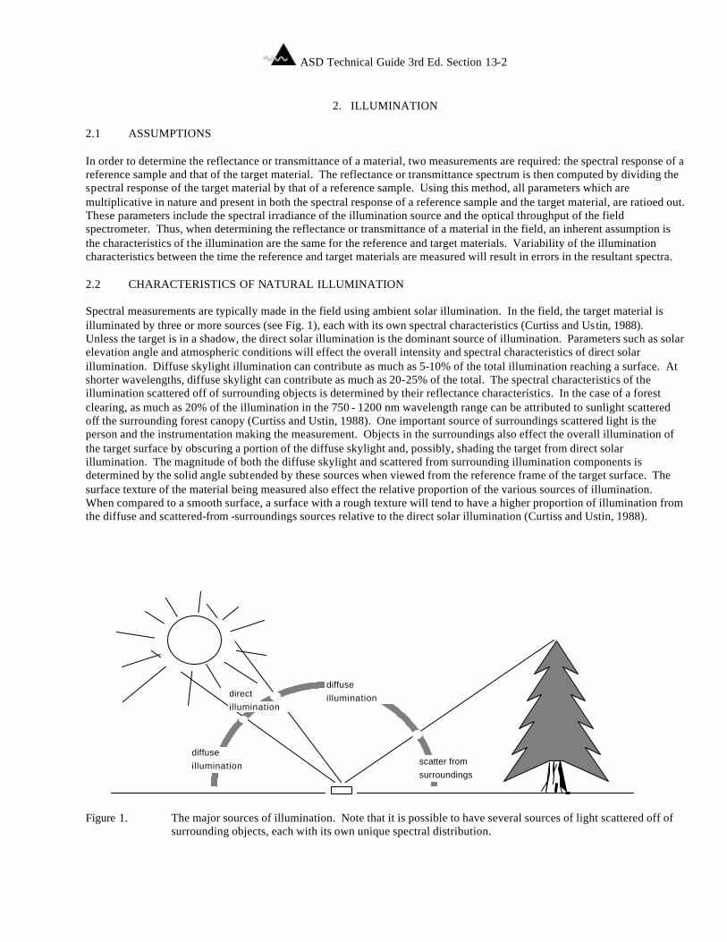
ASD Technical Guide 3rd Ed. Section 13-2
2. ILLUMINATION
2.1 ASSUMPTIONS In order to determine the reflectance or transmittance of a material, two measurements are required: the spectral response of a reference sample and that of the target material. The reflectance or transmittance spectrum is then computed by dividing the spectral response of the target material by that of a reference sample. Using this method, all parameters which are multiplicative in nature and present in both the spectral response of a reference sample and the target material, are ratioed out. These parameters include the spectral irradiance of the illumination source and the optical throughput of the field spectrometer. Thus, when determining the reflectance or transmittance of a material in the field, an inherent assumption is the characteristics of the illumination are the same for the reference and target materials. Variability of the illumination characteristics between the time the reference and target materials are measured will result in errors in the resultant spectra. 2.2 CHARACTERISTICS OF NATURAL ILLUMINATION Spectral measurements are typically made in the field using ambient solar illumination. In the field, the target material is illuminated by three or more sources (see Fig. 1), each with its own spectral characteristics (Curtiss and Ustin, 1988). Unless the target is in a shadow, the direct solar illumination is the dominant source of illumination. Parameters such as solar elevation angle and atmospheric conditions will effect the overall intensity and spectral characteristics of direct solar illumination. Diffuse skylight illumination can contribute as much as 5-10% of the total illumination reaching a surface. At shorter wavelengths, diffuse skylight can contribute as much as 20-25% of the total. The spectral characteristics of the illumination scattered off of surrounding objects is determined by their reflectance characteristics. In the case of a forest clearing, as much as 20% of the illumination in the 750 - 1200 nm wavelength range can be attributed to sunlight scattered off the surrounding forest canopy (Curtiss and Ustin, 1988). One important source of surroundings scattered light is the person and the instrumentation making the measurement. Objects in the surroundings also effect the overall illumination of the target surface by obscuring a portion of the diffuse skylight and, possibly, shading the target from direct solar illumination. The magnitude of both the diffuse skylight and scattered from surrounding illumination components is determined by the solid angle subtended by these sources when viewed from the reference frame of the target surface. The surface texture of the material being measured also effect the relative proportion of the various sources of illumination. When compared to a smooth surface, a surface with a rough texture will tend to have a higher proportion of illumination from the diffuse and scattered-from -surroundings sources relative to the direct solar illumination (Curtiss and Ustin, 1988).
scatter from surroundings
diffuse illumination
diffuse illumination
direct illumination
Figure 1. The major sources of illumination. Note that it is possible to have several sources of light scattered off of
surrounding objects, each with its own unique spectral distribution.
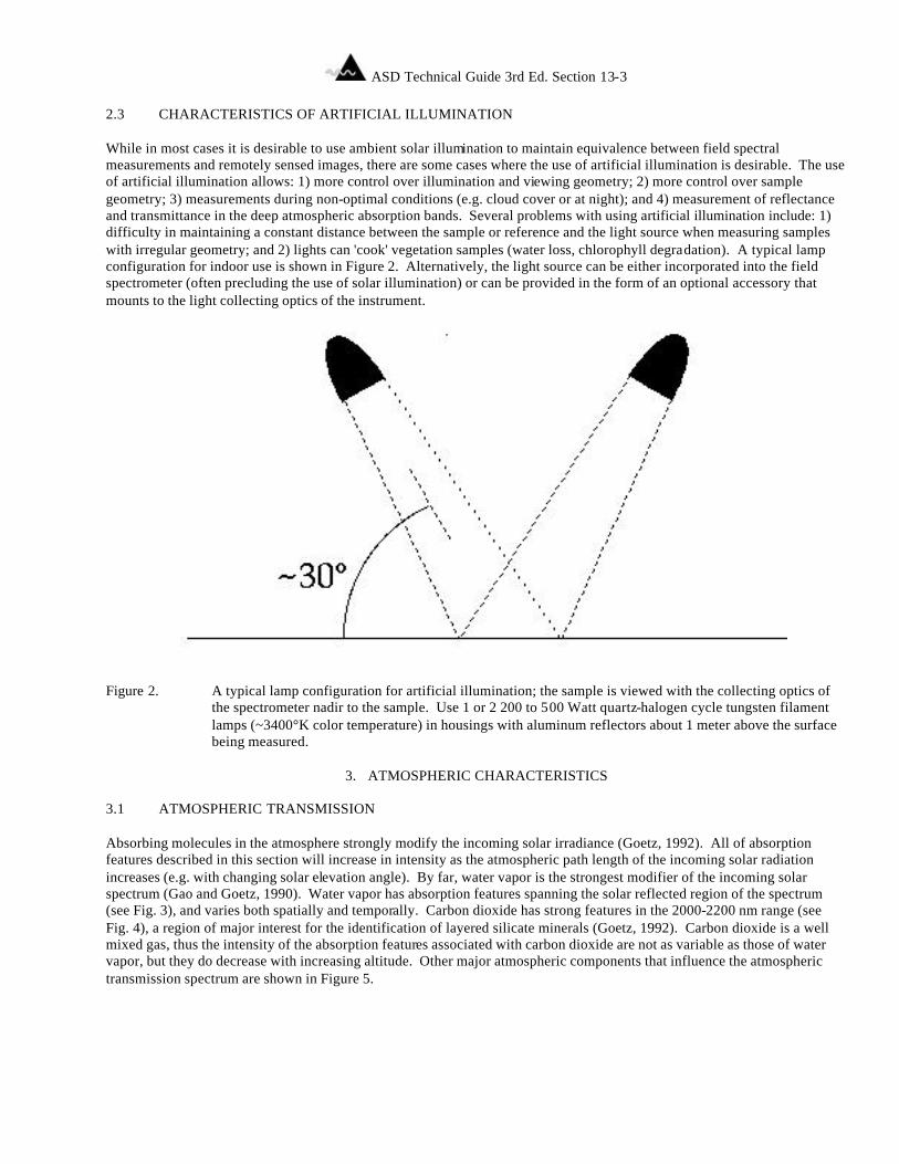
ASD Technical Guide 3rd Ed. Section 13-3
2.3 CHARACTERISTICS OF ARTIFICIAL ILLUMINATION While in most cases it is desirable to use ambient solar illumination to maintain equivalence between field spectral measurements and remotely sensed images, there are some cases where the use of artificial illumination is desirable. The use of artificial illumination allows: 1) more control over illumination and viewing geometry; 2) more control over sample geometry; 3) measurements during non-optimal conditions (e.g. cloud cover or at night); and 4) measurement of reflectance and transmittance in the deep atmospheric absorption bands. Several problems with using artificial illumination include: 1) difficulty in maintaining a constant distance between the sample or reference and the light source when measuring samples with irregular geometry; and 2) lights can 'cook' vegetation samples (water loss, chlorophyll degradation). A typical lamp configuration for indoor use is shown in Figure 2. Alternatively, the light source can be either incorporated into the field spectrometer (often precluding the use of solar illumination) or can be provided in the form of an optional accessory that mounts to the light collecting optics of the instrument.
Figure 2. A typical lamp configuration for artificial illumination; the sample is viewed with the collecting optics of
the spectrometer nadir to the sample. Use 1 or 2 200 to 500 Watt quartz-halogen cycle tungsten filament lamps (~3400°K color temperature) in housings with aluminum reflectors about 1 meter above the surface being measured.
3. ATMOSPHERIC CHARACTERISTICS
3.1 ATMOSPHERIC TRANSMISSION Absorbing molecules in the atmosphere strongly modify the incoming solar irradiance (Goetz, 1992). All of absorption features described in this section will increase in intensity as the atmospheric path length of the incoming solar radiation increases (e.g. with changing solar elevation angle). By far, water vapor is the strongest modifier of the incoming solar spectrum (Gao and Goetz, 1990). Water vapor has absorption features spanning the solar reflected region of the spectrum (see Fig. 3), and varies both spatially and temporally. Carbon dioxide has strong features in the 2000-2200 nm range (see Fig. 4), a region of major interest for the identification of layered silicate minerals (Goetz, 1992). Carbon dioxide is a well mixed gas, thus the intensity of the absorption features associated with carbon dioxide are not as variable as those of water vapor, but they do decrease with increasing altitude. Other major atmospheric components that influence the atmospheric transmission spectrum are shown in Figure 5.
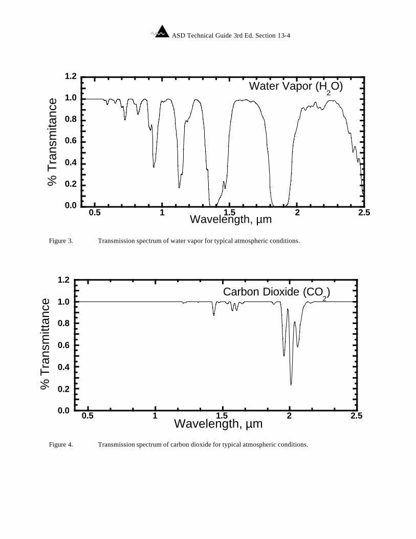
ASD Technical Guide 3rd Ed. Section 13-4
Figure 3. Transmission spectrum of water vapor for typical atmospheric conditions. Figure 4. Transmission spectrum of carbon dioxide for typical atmospheric conditions.
0.0
0.2
0.4
0.6
0.8
1.0
1.2
0.5 1 1.5 2 2.5
Carbon Dioxide (CO2)
% T
rans
mitt
ance
Wavelength, µm
0.0
0.2
0.4
0.6
0.8
1.0
1.2
0.5 1 1.5 2 2.5
% T
rans
mita
nce
Water Vapor (H2O)
Wavelength, µm
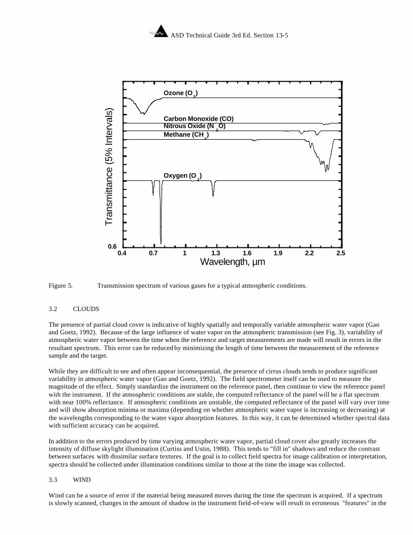
ASD Technical Guide 3rd Ed. Section 13-5
Figure 5. Transmission spectrum of various gases for a typical atmospheric conditions. 3.2 CLOUDS The presence of partial cloud cover is indicative of highly spatially and temporally variable atmospheric water vapor (Gao and Goetz, 1992). Because of the large influence of water vapor on the atmospheric transmission (see Fig. 3), variability of atmospheric water vapor between the time when the reference and target measurements are made will result in errors in the resultant spectrum. This error can be reduced by minimizing the length of time between the measurement of the reference sample and the target. While they are difficult to see and often appear inconsequential, the presence of cirrus clouds tends to produce significant variability in atmospheric water vapor (Gao and Goetz, 1992). The field spectrometer itself can be used to measure the magnitude of the effect. Simply standardize the instrument on the reference panel, then continue to view the reference panel with the instrument. If the atmospheric conditions are stable, the computed reflectance of the panel will be a flat spectrum with near 100% reflectance. If atmospheric conditions are unstable, the computed reflectance of the panel will vary over time and will show absorption minima or maxima (depending on whether atmospheric water vapor is increasing or decreasing) at the wavelengths corresponding to the water vapor absorption features. In this way, it can be determined whether spectral data with sufficient accuracy can be acquired. In addition to the errors produced by time varying atmospheric water vapor, partial cloud cover also greatly increases the intensity of diffuse skylight illumination (Curtiss and Ustin, 1988). This tends to "fill in" shadows and reduce the contrast between surfaces with dissimilar surface textures. If the goal is to collect field spectra for image calibration or interpretation, spectra should be collected under illumination conditions similar to those at the time the image was collected. 3.3 WIND Wind can be a source of error if the material being measured moves during the time the spectrum is acquired. If a spectrum is slowly scanned, changes in the amount of shadow in the instrument field-of-view will result in erroneous "features" in the
0.60.4 0.7 1 1.3 1.6 1.9 2.2 2.5
Tran
smitt
ance
(5%
Inte
rval
s)
Ozone (O3)
Nitrous Oxide (N2O)
Carbon Monoxide (CO)
Methane (CH4)
Oxygen (O2)
Wavelength, µm
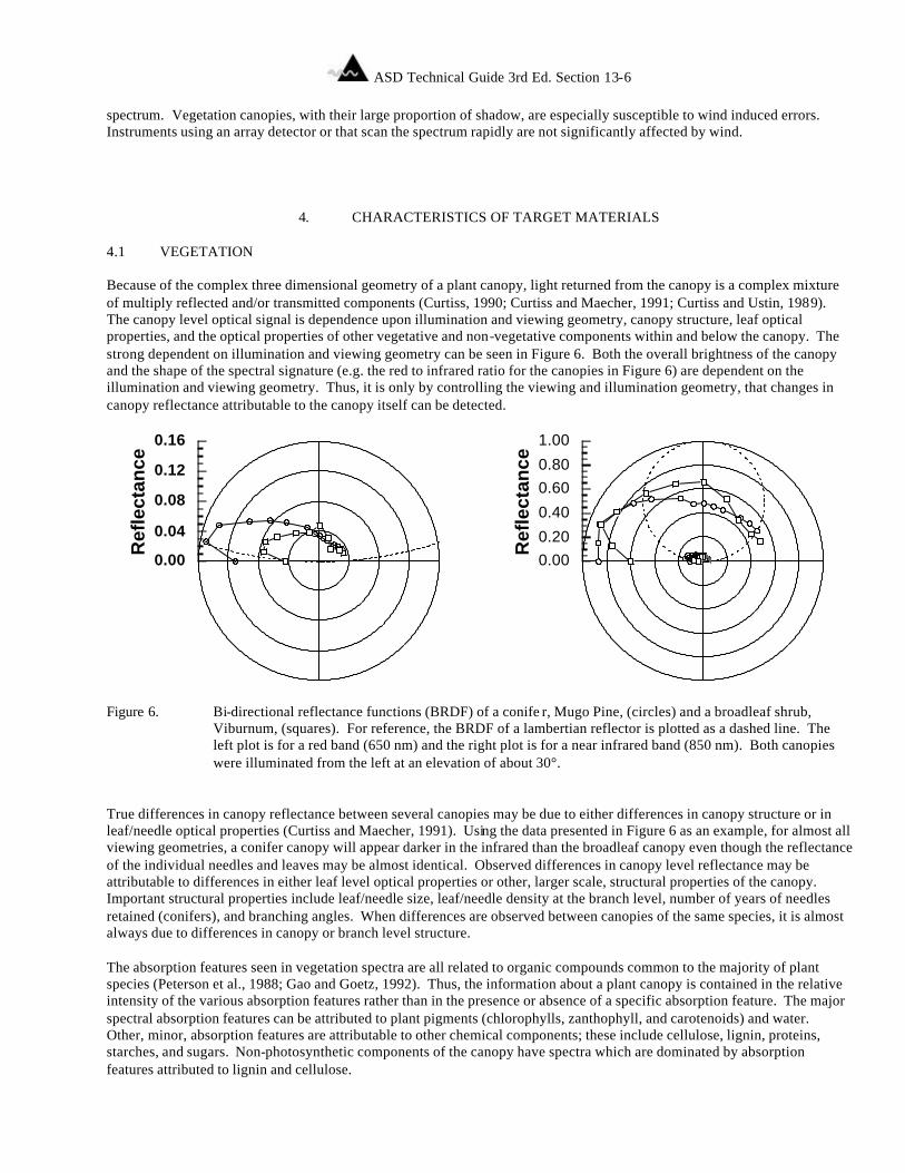
ASD Technical Guide 3rd Ed. Section 13-6
spectrum. Vegetation canopies, with their large proportion of shadow, are especially susceptible to wind induced errors. Instruments using an array detector or that scan the spectrum rapidly are not significantly affected by wind.
4. CHARACTERISTICS OF TARGET MATERIALS 4.1 VEGETATION Because of the complex three dimensional geometry of a plant canopy, light returned from the canopy is a complex mixture of multiply reflected and/or transmitted components (Curtiss, 1990; Curtiss and Maecher, 1991; Curtiss and Ustin, 1989). The canopy level optical signal is dependence upon illumination and viewing geometry, canopy structure, leaf optical properties, and the optical properties of other vegetative and non-vegetative components within and below the canopy. The strong dependent on illumination and viewing geometry can be seen in Figure 6. Both the overall brightness of the canopy and the shape of the spectral signature (e.g. the red to infrared ratio for the canopies in Figure 6) are dependent on the illumination and viewing geometry. Thus, it is only by controlling the viewing and illumination geometry, that changes in canopy reflectance attributable to the canopy itself can be detected. Figure 6. Bi-directional reflectance functions (BRDF) of a conife r, Mugo Pine, (circles) and a broadleaf shrub,
Viburnum, (squares). For reference, the BRDF of a lambertian reflector is plotted as a dashed line. The left plot is for a red band (650 nm) and the right plot is for a near infrared band (850 nm). Both canopies were illuminated from the left at an elevation of about 30°.
True differences in canopy reflectance between several canopies may be due to either differences in canopy structure or in leaf/needle optical properties (Curtiss and Maecher, 1991). Using the data presented in Figure 6 as an example, for almost all viewing geometries, a conifer canopy will appear darker in the infrared than the broadleaf canopy even though the reflectance of the individual needles and leaves may be almost identical. Observed differences in canopy level reflectance may be attributable to differences in either leaf level optical properties or other, larger scale, structural properties of the canopy. Important structural properties include leaf/needle size, leaf/needle density at the branch level, number of years of needles retained (conifers), and branching angles. When differences are observed between canopies of the same species, it is almost always due to differences in canopy or branch level structure. The absorption features seen in vegetation spectra are all related to organic compounds common to the majority of plant species (Peterson et al., 1988; Gao and Goetz, 1992). Thus, the information about a plant canopy is contained in the relative intensity of the various absorption features rather than in the presence or absence of a specific absorption feature. The major spectral absorption features can be attributed to plant pigments (chlorophylls, zanthophyll, and carotenoids) and water. Other, minor, absorption features are attributable to other chemical components; these include cellulose, lignin, proteins, starches, and sugars. Non-photosynthetic components of the canopy have spectra which are dominated by absorption features attributed to lignin and cellulose.
0.00
0.04
0.08
0.12
0.16
Ref
lect
ance
0.000.20
0.40
0.600.80
1.00
Ref
lect
ance
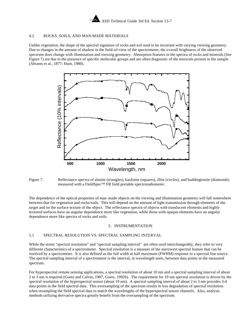
ASD Technical Guide 3rd Ed. Section 13-7
4.2 ROCKS, SOILS, AND MAN-MADE MATERIALS Unlike vegetation, the shape of the spectral signature of rocks and soil tend to be invariant with varying viewing geometry. Due to changes in the amount of shadow in the field-of-view of the spectrometer, the overall brightness of the observed spectrum does change with illumination and viewing geometry. Absorption features in the spectra of rocks and minerals (See Figure 7) are due to the presence of specific molecular groups and are often diagnostic of the minerals present in the sample (Abrams et al., 1877; Hunt, 1980). Figure 7. Reflectance spectra of alunite (triangles), kaolinite (squares), illite (circles), and buddingtonite (diamonds)
measured with a FieldSpec™ FR field portable spectroradiometer. The dependence of the optical properties of man-made objects on the viewing and illumination geometry will fall somewhere between that for vegetation and rocks/soils. This will depend on the amount of light transmission through elements of the target and on the surface texture of the object. The reflectance spectra of objects with translucent elements and highly textured surfaces have an angular dependence more like vegetation, while those with opaque elements have an angular dependence more like spectra of rocks and soils.
5. INSTRUMENTATION 5.1 SPECTRAL RESOLUTION VS. SPECTRAL SAMPLING INTERVAL While the terms "spectral resolution" and "spectral sampling interval" are often used interchangeably, they refer to very different characteristics of a spectrometer. Spectral resolution is a measure of the narrowest spectral feature that can be resolved by a spectrometer. It is also defined as the full width at half maximum (FWHM) response to a spectral line source. The spectral sampling interval of a spectrometer is the interval, in wavelength units, between data points in the measured spectrum. For hyperspectral remote sensing applications, a spectral resolution of about 10 nm and a spectral sampling interval of about 2 to 3 nm is required (Goetz and Calvin, 1987, Goetz, 1992b). The requirement for 10 nm spectral resolution is driven by the spectral resolution of the hyperspectral sensor (about 10 nm). A spectral sampling interval of about 2 to 3 nm provides 3-4 data points in the field spectral data. This oversampling of the spectrum results in less degradation of spectral resolution when resampling the field spectral data to match the wavelengths of the hyperspectral sensor channels. Also, analysis methods utilizing derivative spectra greatly benefit from the oversampling of the spectrum.
500 1000 1500 2000
Ref
lect
ance
(10
% in
terv
als)
Wavelength, nm
ASD Technical Guide 3rd Ed. Section 13-8
5.2 SPECTROMETER DESIGN Spectrometers used in currently available field spectrometers are either based upon a fixed grating and an array detector, or a single element detector and a scanning grating. One of the drawbacks of an array based spectrometer is the signal-to-noise ratio (SNR) is tied to the sampling interval as well as the spectral resolution (Smith, 1992), while in a scanning spectrometer the SNR is independent of spectral sampling interval. Array detectors in the 350 to 1000 nm region of the spectrum (VNIR) have sufficient sensitivity to allow spectra to be collected with spectral resolutions well above the 10 nm resolution required for hyperspectral remote sensing studies. Thus, in the VNIR, fixed grating, array detector, based spectrometers provide the best performance for most remote sensing applications. Typical VNIR spectrometer designs provide 3 to 5 nm spectral resolution with a spectral sampling interval of better than 2 nm. Due to the rapid fall-off in energy of the solar spectrum in the 1000 to 2500 nm region of the spectrum (SWIR), spectrometer design is strongly driven by the need to maintain an acceptable SNR. In general, a loss of SNR is not acceptable in exchange for decreased spectral sampling interval. Thus, the use of an array detector in the SWIR spectral region generally precludes the oversampling of the spectrum. While scanning spectrometers do not have this limitation, they have the drawback of not measuring all wavelengths simultaneously. This can result in errors due to changes in the target during the measurement of the spectrum (see Section 3.3). This limitation is overcome by rapidly scanning the spectrum. Traditionally, scanning SWIR spectrometers have used lead sulfide (PbS) detectors. Due to the lack of sufficient frequency response, the use of PbS detectors precludes rapid scanning. Indium gallium arsinide (InGaAs) detectors have the high frequency response required for rapid scanning (less than 100 milliseconds to scan from 1000 to 2500 nm). InGaAs detectors have the added advantage of having a higher sensitivity than PbS and, also, do not require an optical chopper as does PbS. These increases in performance over PbS allow the design of a rapid scanning spectrometer with equivalent or better SNR performance than a PbS array detector based spectrometer. A scanning design has the added advantage of being having a spectral sampling interval that is less than one fifth the spectral resolution without a reduction in SNR. While it is possible to include the illumination source within the spectrometer, this limits the applications that can be addressed and the types of targets that can be measured. Because of the need to hold illumination and viewing geometry constant between the field and image spectral data, field spectra collected for either hyperspectral sensor calibration or for direct comparison with hyperspectral image data are best collected using ambient solar illumination. The use of a built-in light source also precludes the measurement of radiance or irradiance. Additionally, targets such as vegetation with a complex three dimensional structure can only be measured in the field using solar illumination. 5.3 SPECTROMETER FIELD OF VIEW Existing field spectrometers use one of two basic approaches to collect light energy and deliver it to the spectrometer. In some spectrometer designs, foreoptics are used to form an image of the target upon the entrance slit of the spectrometer. This approach results in a ground field of view (GFOV) that has the same shape as the spectrometer entrance slit (often a rectangle with a height to width ratio of more than 10:1). If more than one spectrometer is used in an instrument (e.g. a VNIR and SWIR spectrometer), it is often difficult to ensure both spectrometers are viewing the same GFOV. The use of optical fibers to deliver the light to the spectrometer results in a circular GFOV. The use of more than one spectrometer is accommodated by splitting the optical fiber bundle within the instrument to deliver light to the various spectrometers. The size of the GFOV is determined by the angular field of view of the instrument and the distance to the target. While optics can be added to modify the angular field of view of a field instrument, this is often practical only for those instruments utilizing optical fibers for light collection.
6. EXPERIMENTAL DESIGN 6.1 TIME OF DAY / YEAR The timing of the field data collection is important if field spectra are to be used to calibrate or interpret a hyperspectral image. Reflectance spectra used to interpret a hyperspectral image should be collected under illumination conditions similar to those when the image was acquired. Time of day and date are the major controlling factors of direct illumination geometry, while atmospheric conditions relating to scattering and clouds are the major factors controlling the geometry and relative intensity of indirect illumination (Curtiss and Ustin, 1988). If field spectra are to be used to convert a hyperspectral sensor image to reflectance, spectra should be acquired simultaneously with image acquisition. If this is not possible, a water vapor correction should be made to the image prior to its conversion to reflectance (Gao and Goetz, 1990).
ASD Technical Guide 3rd Ed. Section 13-9
6.2 SAMPLING STRATEGY The selection of a particular sampling strategy should be based upon the objectives of the study. If the objective is to determine the detectability of either a target material or of a process effecting the spectral signature of a target material, the sampling strategy must encompass examples of the target material under all expected conditions as well as all other background materials. Consideration must be given to all the processes modifying target and background spectral signatures; these include illumination, slope and aspect, and target surface architecture. Adequate collection of vegetation is even more problematic due to the wide range of processes that effect their spectral signature. These include soil chemical properties, soil reflectance, water availability, time of day, time of year, cloud cover, temperature, and relative humidity. If the purpose of a study is to understand how a process effects the spectral signature of a target without consideration of how background materials and other sources of variability effect the spectral signature, variance from sources other than the one of interest should be minimized in the selected targets. This is achieved by carefully controlling viewing and illumination geometry, often in a laboratory. This type of study is often performed as a feasibility study prior to a full study evolving collection of spectra of background material. 6.3 VIEWING GEOMETRY The selection of an appropriate viewing geometry depends upon whether the spectra are used for image analysis or for a feasibility study. For image analysis, a viewing geometry similar to the airborne sensor is required. For a feasibility study it is possible to eliminate much of the confounding variance typically present in an image data set by fixing the viewing and illumination geometry. For vegetation, spectra can be acquired at the spatial scale of the leaf/needle, branch, or canopy. Canopy level spectra are most suitable for image analysis and interpretation. Rarely can leaf/needle or branch level spectra be used to directly to interpret an image. Leaf/needle and branch level spectra are useful to understand how the canopy level spectra are influenced by changes in leaf/needle and branch spectral changes as opposed to changes in the canopy structure. 6.4 ANCILLARY DATA SETS Collection of appropriate ancillary data sets is as important as the collection of field spectra. The measurement of processes and material properties directly influencing, or correlated with, the collected spectra are essential to the understanding of the variance observed in a hyperspectral image data set. It is often necessary to collect a set of spectra with ancillary data in order to validate predictions made using the main field spectra plus image data set.
REFERENCES
Abrams, M.J., R. Ashley, L.C. Rowan, A.F.H. Goetz, and A.B. Kahle (1977) Mapping of hydrothermal alteration in the Cuprite Mining District, Nevada, using aircraft scanner imagery for the 0.46 - 2.36 µm spectral region, Geol., 5, 713-718.
Conel J.E., C.J. Bruegge and B. Curtiss (1987a) Correcting Airborne Imaging Spectrometer measurements for the
atmosphere: a comparison of methods. Proc. 31st. S.P.I.E. International Technical Symposium on Optical and Optoelectronic Applied Science and Engineering.
Conel J.E., R.O. Green, G. Vane, C.J. Bruegge, R.E. Alley and B. Curtiss (1987b) AIS-2 Radiometry and a comparison of
methods for the recovery of ground reflectance. Proc. of the Third Airborne Imaging Spectrometer Data Analysis Workshop..
Curtiss B. (1990) From leaf to landscape: The parameterization of vegetation canopy radiative transfer models from remote
sensing data. Proc. Ann. Meeting of the Ecol. Society of Amer. . Curtiss B. and A.G. Maecher (1991) Changes in forest canopy reflectance associated with chronic exposure to high
concentrations of soil trace metals. Proc. of the 8th Thematic Conference on Geologic Remote Sensing, Denver, Colorado.
Curtiss B. and S.L. Ustin (1988) Spectral changes in Ponderosa Pine associated with natural ozone exposure. Proc. U.S.
Forest Service Forest Response Program Annual Meeting, Corpus Christi, Texas, February 23 - 26.

ASD Technical Guide 3rd Ed. Section 13-10
Curtiss B. and S.L. Ustin (1989a) The Remote Detection of Early Stages of Air Pollution Injury in Coniferous Forests using
imaging Spectrometry. Proc. European Joint Research Center Remote Sensing of Forests Workshop. Ispara, Italy. Gao, B.-C. and A.F.H. Goetz (1990) Column atmospheric water vapor retrievals from airborne imaging spectrometer data,
J. Geophys. Res.-Atmospheres, 95, 3549-3564. Gao, B.-C., and A.F.H. Goetz (1992) A Linear Spectral Matching Technique for Retrieving Equivalent Water Thickness and
Biochemical Constituents of Green Vegetation, Proc. of the Third Airborne Annual JPL Geoscience Workshop (AVIRIS, TIMS, and AIRSAR), Jet Propulsion Laboratory, Pasadena, CA.
Goetz, A.F.H. (1992a) Imaging Spectrometry for Earth Remote Sensing, in Imaging Spectroscopy: Fundamentals and
Prospective Applications, F. Toselli and J. Bodechtel, Eds., pp. 1-19, Brussels and Luxembourg. Goetz, A.F.H. (1992b) Principles of Narrow Band Spectrometry, in The Visible and IR: Instruments and Data Analysis in
Imaging Spectroscopy: Fundamentals and Prospective Applications, F. Toselli and J. Bodechtel, Eds., pp. 21-32, Brussels and Luxembourg.
Goetz, A.F.H. and W.M. Calvin (1987) Imaging spectrometry: Spectral resolution and analytical identification of spectral
features, Imaging Spectros. II, G.Vane, Ed., Proc. SPIE , 834, 158-165. Goetz, A.F.H. and V. Srivastava (1985) Mineralogical mapping in the Cuprite mining district, Nevada, Proceedings of the
Airborne Imaging Spectrometer Data Analysis Workshop, April 1985, JPL Publication , no. 85-41. Hunt, G.R. (1980) Electromagnetic radiation: The communications link in remote sensing. In Remote Sensing in Geology,
B.S. Siegal and A.R. Gillespie, eds, Wiley, NY, pp 5-45. Peterson, D.L., J.D. Aber, P.A. Matson, D.H. Card, N. Swanberg, C.A. Wessman and M. Spanner (1988) Remote sensing of
forest canopy and leaf biochemical contnets, Rem. Sens. Environ., 24, 85-108. Smith, M.W. (1992) Design and initial performance evaluation of a portable short wave infrared spectrometer, Proc. SPIE,
Vol. 1762-14., San Diego, CA.
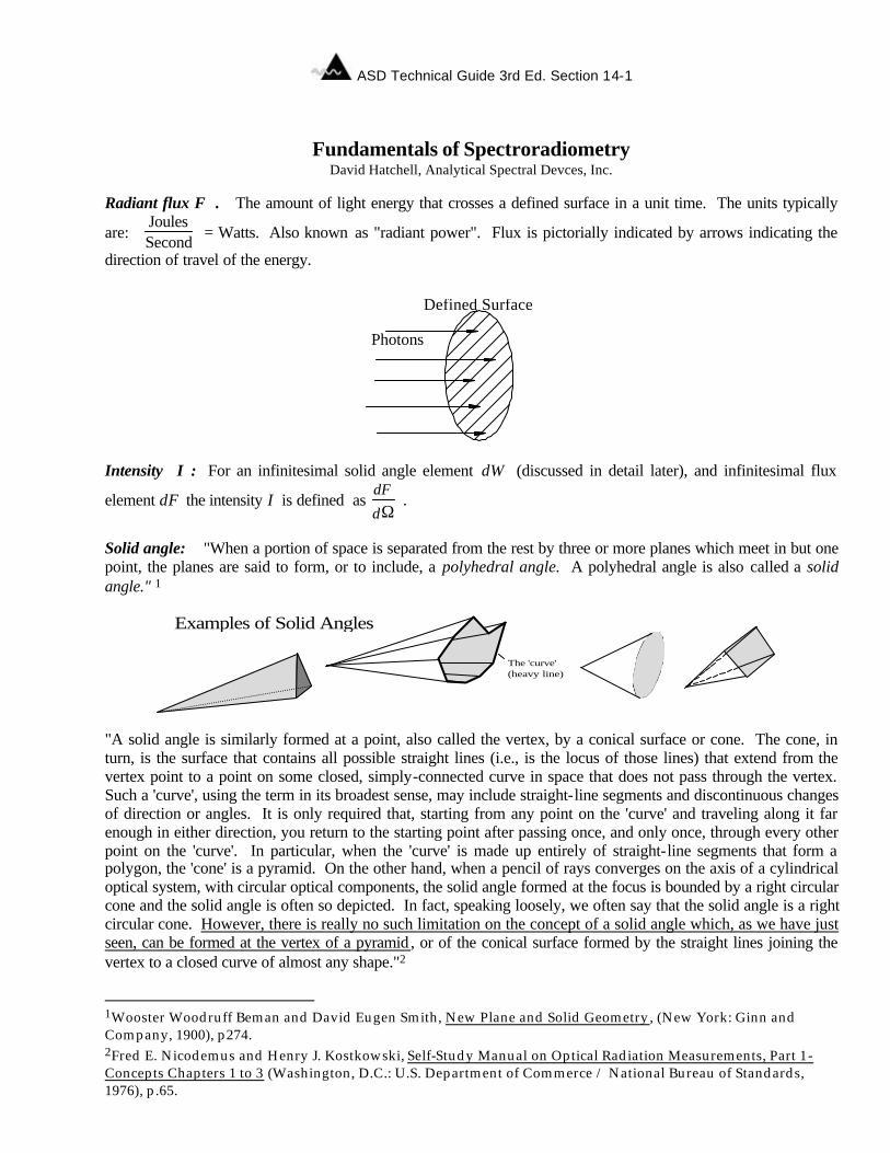
ASD Technical Guide 3rd Ed. Section 14-1
Section 14 Fundamentals of Spectroradiometry
Fundamentals of Spectroradiometry David Hatchell, Analytical Spectral Devces, Inc.
Radiant flux F . The amount of light energy that crosses a defined surface in a unit time. The units typically
are: JoulesSecond
= Watts. Also known as "radiant power". Flux is pictorially indicated by arrows indicating the
direction of travel of the energy.
Intensity I : For an infinitesimal solid angle element dΩ (discussed in detail later), and infinitesimal flux
element dF the intensity I is defined as dF
dΩ .
Solid angle: "When a portion of space is separated from the rest by three or more planes which meet in but one point, the planes are said to form, or to include, a polyhedral angle. A polyhedral angle is also called a solid angle." 1
"A solid angle is similarly formed at a point, also called the vertex, by a conical surface or cone. The cone, in turn, is the surface that contains all possible straight lines (i.e., is the locus of those lines) that extend from the vertex point to a point on some closed, simply-connected curve in space that does not pass through the vertex. Such a 'curve', using the term in its broadest sense, may include straight-line segments and discontinuous changes of direction or angles. It is only required that, starting from any point on the 'curve' and traveling along it far enough in either direction, you return to the starting point after passing once, and only once, through every other point on the 'curve'. In particular, when the 'curve' is made up entirely of straight-line segments that form a polygon, the 'cone' is a pyramid. On the other hand, when a pencil of rays converges on the axis of a cylindrical optical system, with circular optical components, the solid angle formed at the focus is bounded by a right circular cone and the solid angle is often so depicted. In fact, speaking loosely, we often say that the solid angle is a right circular cone. However, there is really no such limitation on the concept of a solid angle which, as we have just seen, can be formed at the vertex of a pyramid , or of the conical surface formed by the straight lines joining the vertex to a closed curve of almost any shape."2
1Wooster Woodruff Beman and David Eugen Smith, New Plane and Solid Geometry, (New York: Ginn and Company, 1900), p274. 2Fred E. Nicodemus and Henry J. Kostkowski, Self-Study Manual on Optical Radiation Measurements, Part 1-Concepts Chapters 1 to 3 (Washington, D.C.: U.S. Department of Commerce / National Bureau of Standards, 1976), p.65.
Photons
Defined Surface
Examples of Solid Angles
The 'curve' (heavy line)
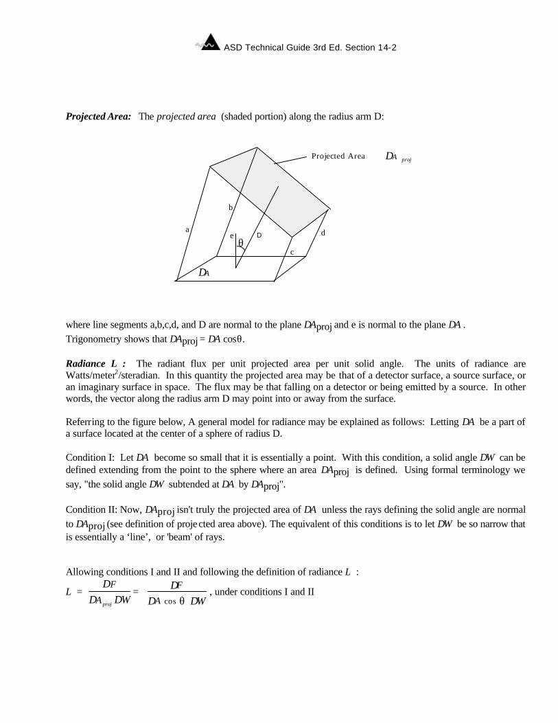
ASD Technical Guide 3rd Ed. Section 14-2
Projected Area: The projected area (shaded portion) along the radius arm D:
Da
b
c
dθ
e
∆A
Projected Area ∆A proj
where line segments a,b,c,d, and D are normal to the plane ∆Aproj and e is normal to the plane ∆A . Trigonometry shows that ∆Aproj = ∆A cosθ. Radiance L : The radiant flux per unit projected area per unit solid angle. The units of radiance are Watts/meter2/steradian. In this quantity the projected area may be that of a detector surface, a source surface, or an imaginary surface in space. The flux may be that falling on a detector or being emitted by a source. In other words, the vector along the radius arm D may point into or away from the surface. Referring to the figure below, A general model for radiance may be explained as follows: Letting ∆A be a part of a surface located at the center of a sphere of radius D. Condition I: Let ∆A become so small that it is essentially a point. With this condition, a solid angle ∆Ω can be defined extending from the point to the sphere where an area ∆Aproj is defined. Using formal terminology we say, "the solid angle ∆Ω subtended at ∆A by ∆Aproj". Condition II: Now, ∆Aproj isn't truly the projected area of ∆A unless the rays defining the solid angle are normal to ∆Aproj (see definition of projected area above). The equivalent of this conditions is to let ∆Ω be so narrow that is essentially a ‘line’, or 'beam' of rays. Allowing conditions I and II and following the definition of radiance L :
L = ∆F
∆A proj ∆Ω=
∆F
∆A cos θ ∆Ω, under conditions I and II
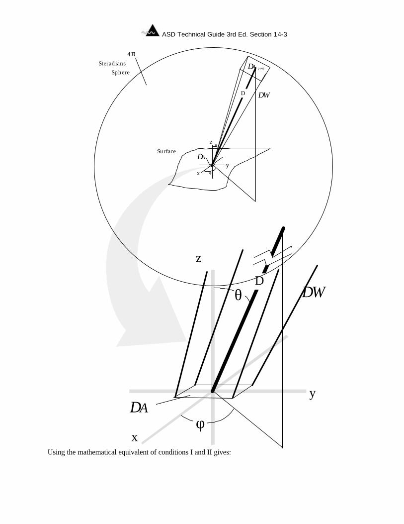
ASD Technical Guide 3rd Ed. Section 14-3
xy
z
D
x
y
z
∆A
θ
∆Ω
∆Ω
Surface
D
φ
4 π
Steradians Sphere
θ
∆A proj
φ
∆A
Using the mathematical equivalent of conditions I and II gives:
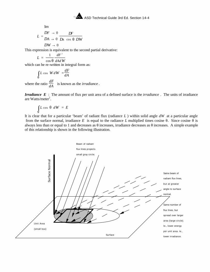
ASD Technical Guide 3rd Ed. Section 14-4
L =
lim
∆F → 0
∆A → 0
∆Ω → 0
∆F
∆A cos θ ∆Ω
This expression is equivalent to the second partial derivative:
L = 1
cos θdF 2
dAd Ω
which can be re-written in integral form as:
L cos Ω dΩΩ∫ =
dFdA
where the ratio dFdA
is known as the irradiance .
Irradiance E : The amount of flux per unit area of a defined surface is the irradiance . The units of irradiance are Watts/meter2.
⇒
L cos θ dΩΩ∫ = E
It is clear that for a particular ‘beam’ of radiant flux (radiance L ) within solid angle dΩ at a particular angle from the surface normal, irradiance E is equal to the radiance L multiplied times cosine θ. Since cosine θ is always less than or equal to 1 and decreases as θ increases, irradiance decreases as θ increases. A simple example of this relationship is shown in the following illustration.
Same beam of
radiant flux lines,
but at greater
angle to surface
normal.
Same number of
flux lines, but
spread over larger
area (large circle).
Ie., lower energy
per unit area. Ie.,
lower irradiance. Surface
Sur
face
Nor
mal
Beam of radiant
flux lines projects
small gray circle.
Unit Area
(small box)
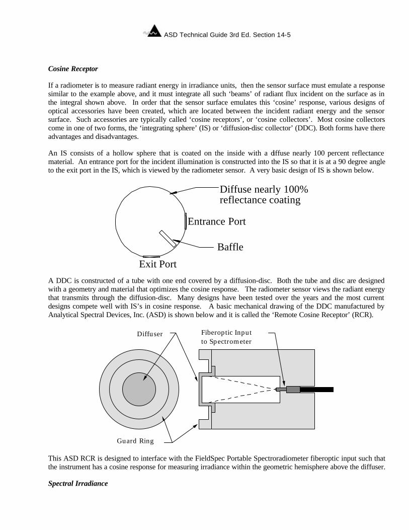
ASD Technical Guide 3rd Ed. Section 14-5
Cosine Receptor If a radiometer is to measure radiant energy in irradiance units, then the sensor surface must emulate a response similar to the example above, and it must integrate all such ‘beams’ of radiant flux incident on the surface as in the integral shown above. In order that the sensor surface emulates this ‘cosine’ response, various designs of optical accessories have been created, which are located between the incident radiant energy and the sensor surface. Such accessories are typically called ‘cosine receptors’, or ‘cosine collectors’. Most cosine collectors come in one of two forms, the ‘integrating sphere’ (IS) or ‘diffusion-disc collector’ (DDC). Both forms have there advantages and disadvantages. An IS consists of a hollow sphere that is coated on the inside with a diffuse nearly 100 percent reflectance material. An entrance port for the incident illumination is constructed into the IS so that it is at a 90 degree angle to the exit port in the IS, which is viewed by the radiometer sensor. A very basic design of IS is shown below.
A DDC is constructed of a tube with one end covered by a diffusion-disc. Both the tube and disc are designed with a geometry and material that optimizes the cosine response. The radiometer sensor views the radiant energy that transmits through the diffusion-disc. Many designs have been tested over the years and the most current designs compete well with IS’s in cosine response. A basic mechanical drawing of the DDC manufactured by Analytical Spectral Devices, Inc. (ASD) is shown below and it is called the ‘Remote Cosine Receptor’ (RCR).
Fiberoptic Inputto Spectrometer
Diffuser
Guard Ring This ASD RCR is designed to interface with the FieldSpec Portable Spectroradiometer fiberoptic input such that the instrument has a cosine response for measuring irradiance within the geometric hemisphere above the diffuser. Spectral Irradiance
Entrance Port
Exit Port
Baffle
Diffuse nearly 100% reflectance coating
ASD Technical Guide 3rd Ed. Section 14-6
For simplicity the above discussions on irradiance have neglected the concept of wavelength interval or ‘band’. A ‘broad-band’ radiometer measures the sum total of integrated irradiances over all wavelengths within the band. Such a radiometer does not discriminate the integrated radiances for discrete wavelength channels or ‘narrow-bands’. A ‘spectro-radiometer’ such as the ASD FieldSpec Portable Spectroradiometer measures the integrated irradiance for many contiguous discrete wavelength channels, all within a single scan. This kind of irradiance measurement is called ‘spectral irradiance’ since the discrete values are stored and displayed as a spectral plot of irradiance versus wavelength. Spectral irradiance has units Watts/meter2/nanometer, which indicates that a discrete irradiance integration is measured for each discrete narrow-band interval of one nanometer. Its is also possible to emulate the broad-band radiometer using a spectro-radiometer, assuming the total spectral range is compatable. This can be done by integrating under the spectral curve of the spectro-radiometer in post processing. Spectral Radiance A spectro-radiometer such as the ASD FieldSpec Portable Spectroradiometer also measures ‘spectral radiance’ for contiguous discrete narrow band intervals of one nanometer and the units of spectral radiance are, Watts/meter2/steradian/nanometer. Either the bare fiberoptic cable or a variety of optional Field-of-View Lens Foreoptics can be used with the ASD FieldSpec Portable Spectroradiometer for measuring radiance. Radiometric Calibrations One other area of detector response not covered in this paper, is the absolute radiometric response. That is, when the spectro-radiometer sensor says that it is measuring one Watt/ meter2/nanometer, it is in fact measuring such a value to within some known error. This area involves ‘radiometric calibration’, which relates the spectro-radiometer sensor real response to a know, traceable calibration standard. ASD uses NIST traceable irradiance standards for creating its radiance and irradiance calibration files for the ASD FieldSpec Portable Spectroradiometer. The procedures and other information regarding these radiometric calibration files are discussed in great detail in the ASD FieldSpec Portable Spectroradiometer User’s Guide.
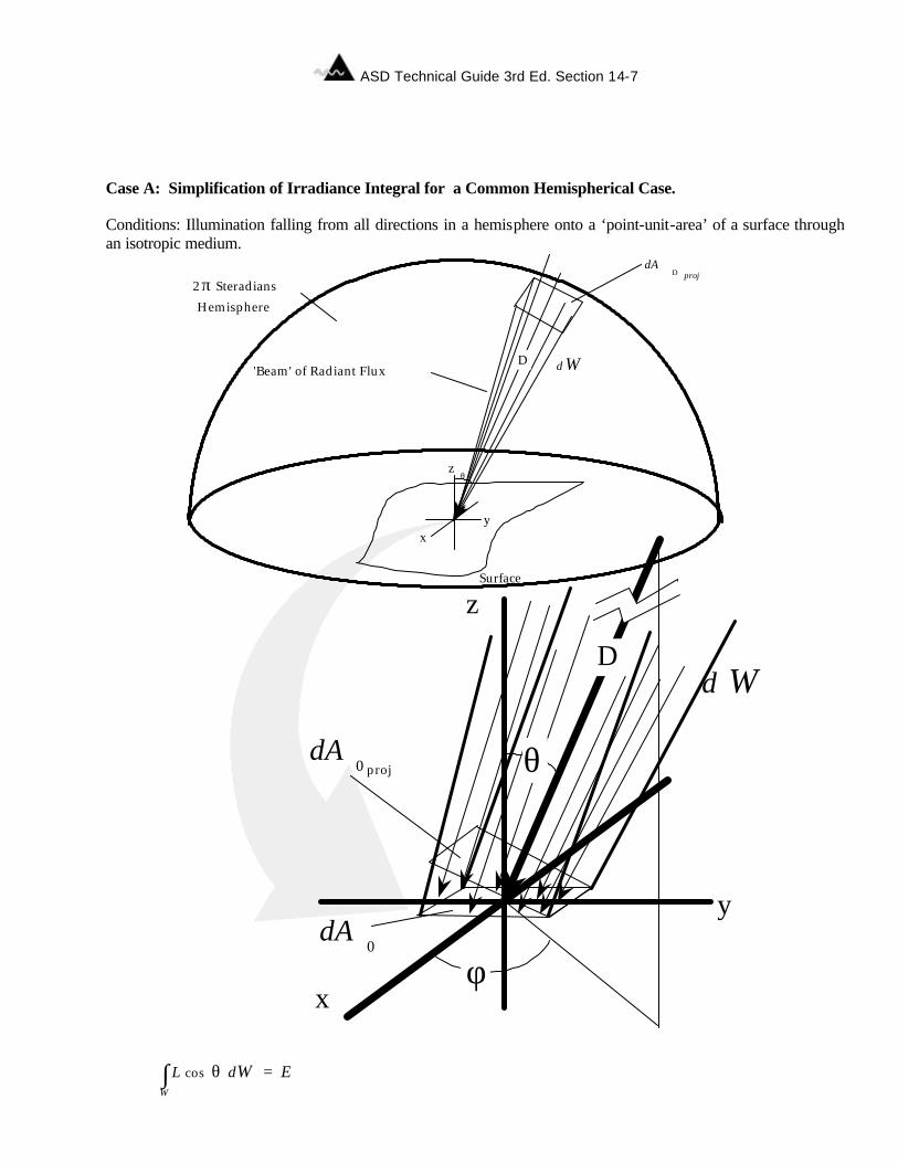
ASD Technical Guide 3rd Ed. Section 14-7
Case A: Simplification of Irradiance Integral for a Common Hemispherical Case. Conditions: Illumination falling from all directions in a hemisphere onto a ‘point-unit-area’ of a surface through an isotropic medium.
xy
z
D
x
y
z
θdA0 proj
dA0
dAD
θ
d Ω
d Ω
Surface
D
φ
'Beam' of Radiant Flux
2 π Steradians
Hemisphere
proj
L cos θ dΩΩ∫ = E
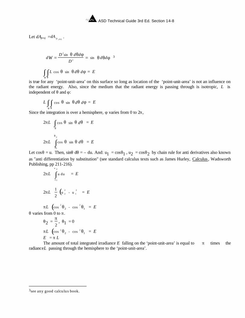
ASD Technical Guide 3rd Ed. Section 14-8
Let dAproj =
dAD proj
.
⇒
dΩ =D 2sin θ dθdφ
D 2= sin θ dθdφ
3
⇒
L cos θ sin θ dθ dφθ∫
φ∫ = E
is true for any ‘point-unit-area’ on this surface so long as location of the ‘point-unit-area’ is not an influence on the radiant energy. Also, since the medium that the radiant energy is passing through is isotropic, L is independent of θ and φ:
⇒ L
cos θ sin θ dθ dφθ∫
φ∫ = E
Since the integration is over a hemisphere, φ varies from 0 to 2π,
⇒ 2πL
cos θ sin θ dθθ∫ = E
⇒ 2πL
cos θ sin θ dθθ1
θ 2
∫ = E
Let cosθ = u. Then, sinθ dθ = – du. And: u1 = cosθ1 , u2 = cosθ2 by chain rule for anti derivatives also known
as "anti differentiation by substitution" (see standard calculus texts such as James Hurley, Calculus , Wadsworth Publishing, pp 211-216).
⇒ 2πL
u duu1
u 2
∫ = E
⇒ 2πL 1
2
u 2
2 - u 1
2( ) = E
⇒ πL
cos2 θ2 - cos
2 θ1( ) = E θ varies from 0 to π.
⇒ θ2 = π2
, θ1 = 0
⇒ πL
cos 2 θ2 - cos 2 θ1( ) = E ⇒ E = π L ⇒ The amount of total integrated irradiance E falling on the ‘point-unit-area’ is equal to π times the radianceL passing through the hemisphere to the ‘point-unit-area’.
3see any good calculus book.
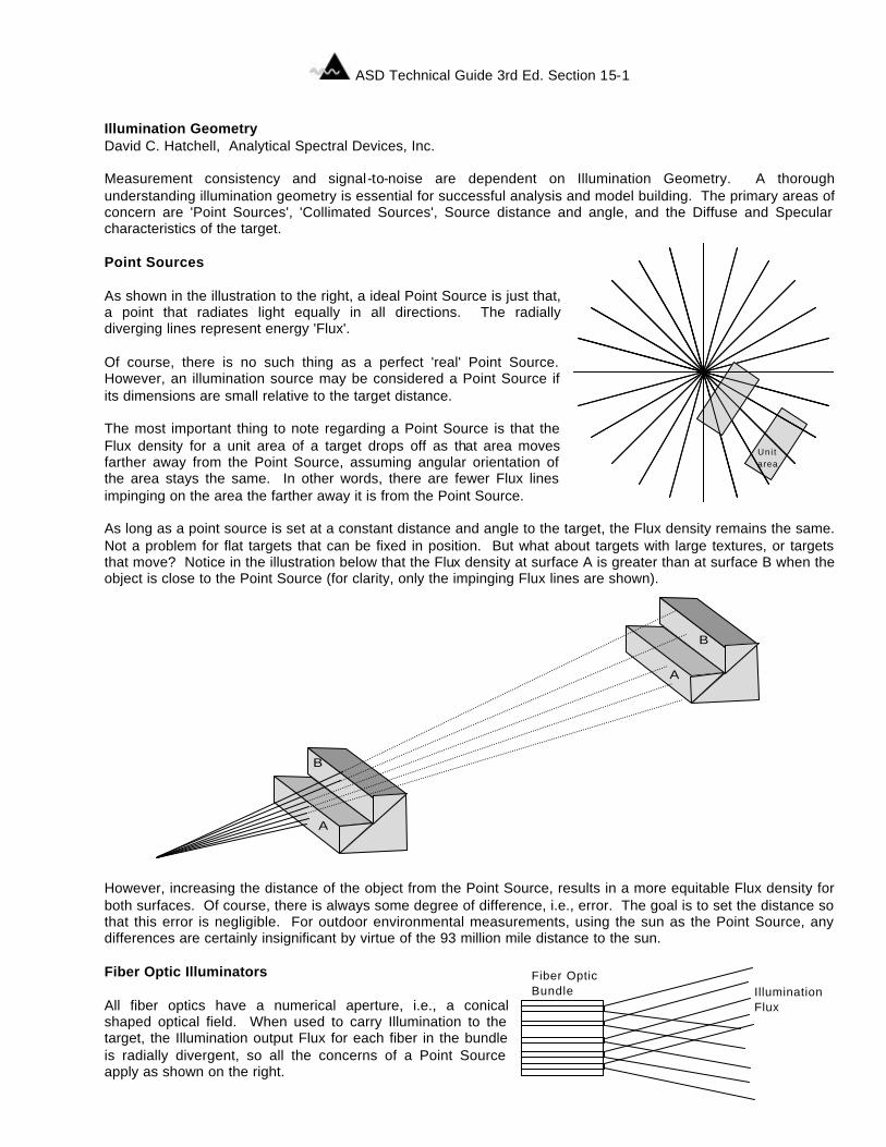
ASD Technical Guide 3rd Ed. Section 15-1
Uni t area
Section 15 Illumination Geometry David C. Hatchell, Analytical Spectral Devices, Inc. Measurement consistency and signal-to-noise are dependent on Illumination Geometry. A thorough understanding illumination geometry is essential for successful analysis and model building. The primary areas of concern are 'Point Sources', 'Collimated Sources', Source distance and angle, and the Diffuse and Specular characteristics of the target. Point Sources As shown in the illustration to the right, a ideal Point Source is just that, a point that radiates light equally in all directions. The radially diverging lines represent energy 'Flux'. Of course, there is no such thing as a perfect 'real' Point Source. However, an illumination source may be considered a Point Source if its dimensions are small relative to the target distance. The most important thing to note regarding a Point Source is that the Flux density for a unit area of a target drops off as that area moves farther away from the Point Source, assuming angular orientation of the area stays the same. In other words, there are fewer Flux lines impinging on the area the farther away it is from the Point Source. As long as a point source is set at a constant distance and angle to the target, the Flux density remains the same. Not a problem for flat targets that can be fixed in position. But what about targets with large textures, or targets that move? Notice in the illustration below that the Flux density at surface A is greater than at surface B when the object is close to the Point Source (for clarity, only the impinging Flux lines are shown).
However, increasing the distance of the object from the Point Source, results in a more equitable Flux density for both surfaces. Of course, there is always some degree of difference, i.e., error. The goal is to set the distance so that this error is negligible. For outdoor environmental measurements, using the sun as the Point Source, any differences are certainly insignificant by virtue of the 93 million mile distance to the sun. Fiber Optic Illuminators All fiber optics have a numerical aperture, i.e., a conical shaped optical field. When used to carry Illumination to the target, the Illumination output Flux for each fiber in the bundle is radially divergent, so all the concerns of a Point Source apply as shown on the right.
A
B
A
B
Illumination Flux
Fiber OpticBundle
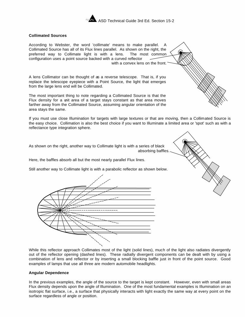
ASD Technical Guide 3rd Ed. Section 15-2
Collimated Sources According to Webster, the word 'collimate' means to make parallel. A Collimated Source has all of its Flux lines parallel. As shown on the right, the preferred way to Collimate light is with a lens. The most common configuration uses a point source backed with a curved reflector
with a convex lens on the front. A lens Collimator can be thought of as a reverse telescope. That is, if you replace the telescope eyepiece with a Point Source, the light that emerges from the large lens end will be Collimated. The most important thing to note regarding a Collimated Source is that the Flux density for a unit area of a target stays constant as that area moves farther away from the Collimated Source, assuming angular orientation of the area stays the same. If you must use close Illumination for targets with large textures or that are moving, then a Collimated Source is the easy choice. Collimation is also the best choice if you want to Illuminate a limited area or 'spot' such as with a reflectance type integration sphere.
As shown on the right, another way to Collimate light is with a series of black absorbing baffles.
Here, the baffles absorb all but the most nearly parallel Flux lines. Still another way to Collimate light is with a parabolic reflector as shown below.
While this reflector approach Collimates most of the light (solid lines), much of the light also radiates divergently out of the reflector opening (dashed lines). These radially divergent components can be dealt with by using a combination of lens and reflector or by inserting a small blocking baffle just in front of the point source. Good examples of lamps that use all three are modern automobile headlights. Angular Dependence In the previous examples, the angle of the source to the target is kept constant. However, even with small areas Flux density depends upon the angle of Illumination. One of the most fundamental examples is Illumination on an isotropic flat surface, i.e., a surface that physically interacts with light exactly the same way at every point on the surface regardless of angle or position.
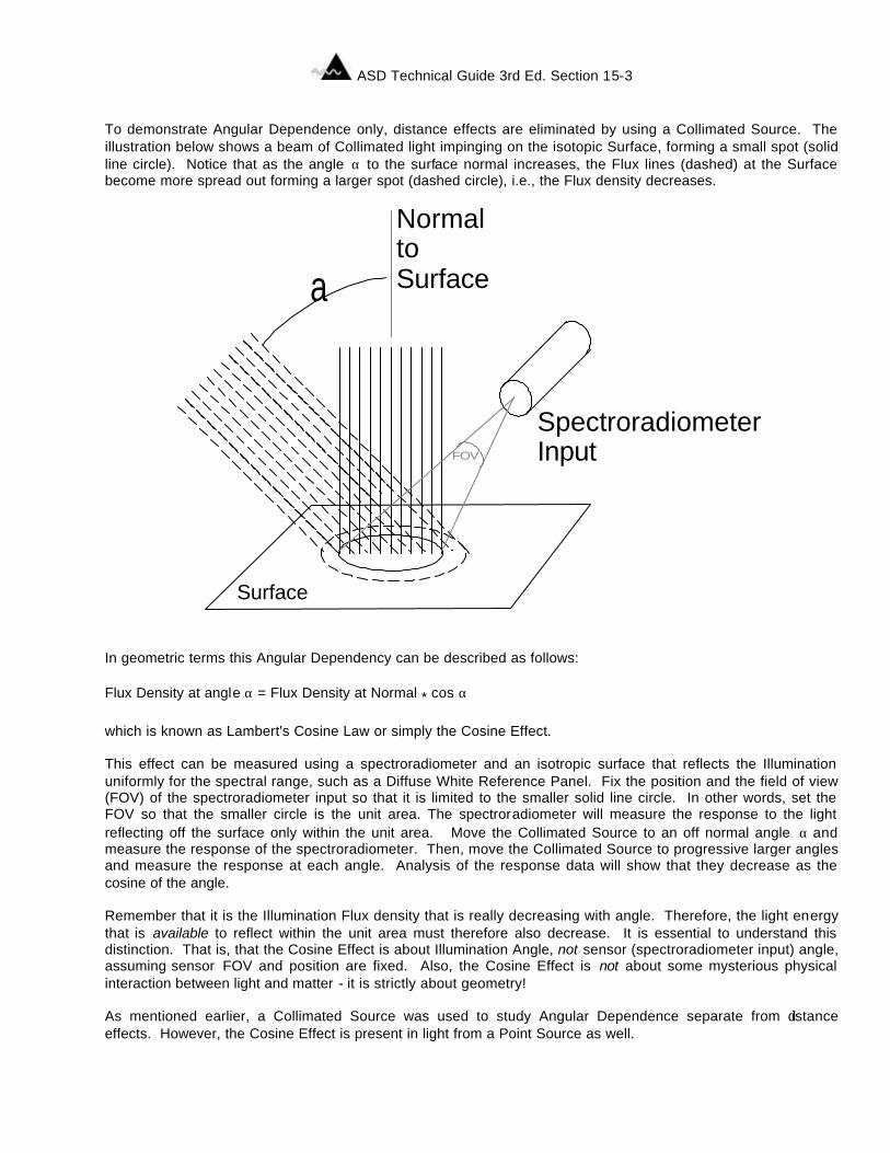
ASD Technical Guide 3rd Ed. Section 15-3
To demonstrate Angular Dependence only, distance effects are eliminated by using a Collimated Source. The illustration below shows a beam of Collimated light impinging on the isotopic Surface, forming a small spot (solid line circle). Notice that as the angle α to the surface normal increases, the Flux lines (dashed) at the Surface become more spread out forming a larger spot (dashed circle), i.e., the Flux density decreases.
In geometric terms this Angular Dependency can be described as follows: Flux Density at angle α = Flux Density at Normal * cos α which is known as Lambert's Cosine Law or simply the Cosine Effect. This effect can be measured using a spectroradiometer and an isotropic surface that reflects the Illumination uniformly for the spectral range, such as a Diffuse White Reference Panel. Fix the position and the field of view (FOV) of the spectroradiometer input so that it is limited to the smaller solid line circle. In other words, set the FOV so that the smaller circle is the unit area. The spectroradiometer will measure the response to the light reflecting off the surface only within the unit area. Move the Collimated Source to an off normal angle α and measure the response of the spectroradiometer. Then, move the Collimated Source to progressive larger angles and measure the response at each angle. Analysis of the response data will show that they decrease as the cosine of the angle. Remember that it is the Illumination Flux density that is really decreasing with angle. Therefore, the light energy that is available to reflect within the unit area must therefore also decrease. It is essential to understand this distinction. That is, that the Cosine Effect is about Illumination Angle, not sensor (spectroradiometer input) angle, assuming sensor FOV and position are fixed. Also, the Cosine Effect is not about some mysterious physical interaction between light and matter - it is strictly about geometry! As mentioned earlier, a Collimated Source was used to study Angular Dependence separate from distance effects. However, the Cosine Effect is present in light from a Point Source as well.
SpectroradiometerInput
NormaltoSurface
FOV
Surface
a
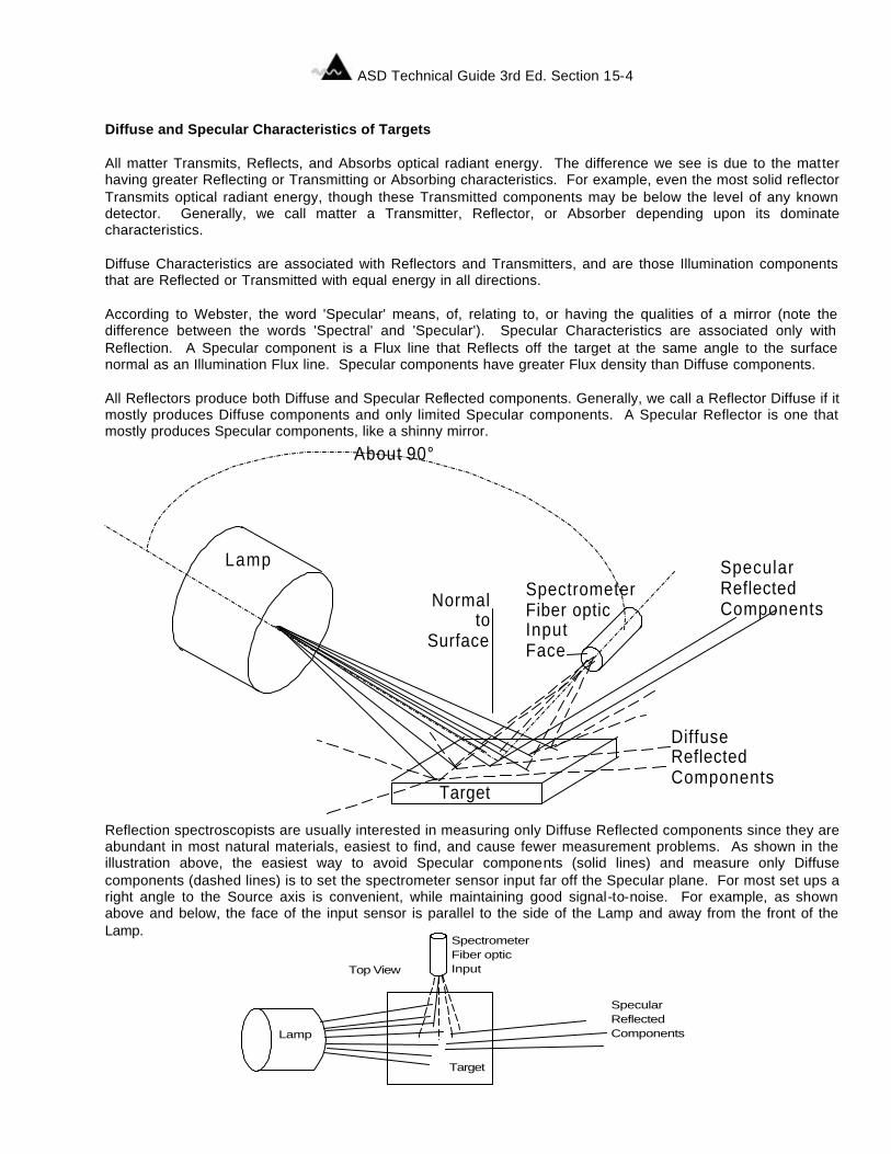
ASD Technical Guide 3rd Ed. Section 15-4
Diffuse and Specular Characteristics of Targets All matter Transmits, Reflects, and Absorbs optical radiant energy. The difference we see is due to the matter having greater Reflecting or Transmitting or Absorbing characteristics. For example, even the most solid reflector Transmits optical radiant energy, though these Transmitted components may be below the level of any known detector. Generally, we call matter a Transmitter, Reflector, or Absorber depending upon its dominate characteristics. Diffuse Characteristics are associated with Reflectors and Transmitters, and are those Illumination components that are Reflected or Transmitted with equal energy in all directions. According to Webster, the word 'Specular' means, of, relating to, or having the qualities of a mirror (note the difference between the words 'Spectral' and 'Specular'). Specular Characteristics are associated only with Reflection. A Specular component is a Flux line that Reflects off the target at the same angle to the surface normal as an Illumination Flux line. Specular components have greater Flux density than Diffuse components. All Reflectors produce both Diffuse and Specular Reflected components. Generally, we call a Reflector Diffuse if it mostly produces Diffuse components and only limited Specular components. A Specular Reflector is one that mostly produces Specular components, like a shinny mirror.
Reflection spectroscopists are usually interested in measuring only Diffuse Reflected components since they are abundant in most natural materials, easiest to find, and cause fewer measurement problems. As shown in the illustration above, the easiest way to avoid Specular components (solid lines) and measure only Diffuse components (dashed lines) is to set the spectrometer sensor input far off the Specular plane. For most set ups a right angle to the Source axis is convenient, while maintaining good signal-to-noise. For example, as shown above and below, the face of the input sensor is parallel to the side of the Lamp and away from the front of the Lamp.
About 90°
Lamp
SpectrometerFiber opticInputFace
Target
SpecularReflectedComponents
DiffuseReflectedComponents
Normalto
Surface
Lamp
SpecularReflectedComponents
Top View
Target
SpectrometerFiber opticInput
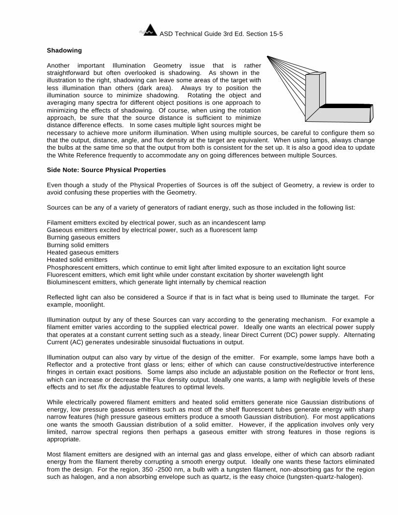
ASD Technical Guide 3rd Ed. Section 15-5
Shadowing Another important Illumination Geometry issue that is rather straightforward but often overlooked is shadowing. As shown in the illustration to the right, shadowing can leave some areas of the target with less illumination than others (dark area). Always try to position the illumination source to minimize shadowing. Rotating the object and averaging many spectra for different object positions is one approach to minimizing the effects of shadowing. Of course, when using the rotation approach, be sure that the source distance is sufficient to minimize distance difference effects. In some cases multiple light sources might be necessary to achieve more uniform illumination. When using multiple sources, be careful to configure them so that the output, distance, angle, and flux density at the target are equivalent. When using lamps, always change the bulbs at the same time so that the output from both is consistent for the set up. It is also a good idea to update the White Reference frequently to accommodate any on going differences between multiple Sources. Side Note: Source Physical Properties Even though a study of the Physical Properties of Sources is off the subject of Geometry, a review is order to avoid confusing these properties with the Geometry. Sources can be any of a variety of generators of radiant energy, such as those included in the following list: Filament emitters excited by electrical power, such as an incandescent lamp Gaseous emitters excited by electrical power, such as a fluorescent lamp Burning gaseous emitters Burning solid emitters Heated gaseous emitters Heated solid emitters Phosphorescent emitters, which continue to emit light after limited exposure to an excitation light source Fluorescent emitters, which emit light while under constant excitation by shorter wavelength light Bioluminescent emitters, which generate light internally by chemical reaction Reflected light can also be considered a Source if that is in fact what is being used to Illuminate the target. For example, moonlight. Illumination output by any of these Sources can vary according to the generating mechanism. For example a filament emitter varies according to the supplied electrical power. Ideally one wants an electrical power supply that operates at a constant current setting such as a steady, linear Direct Current (DC) power supply. Alternating Current (AC) generates undesirable sinusoidal fluctuations in output. Illumination output can also vary by virtue of the design of the emitter. For example, some lamps have both a Reflector and a protective front glass or lens; either of which can cause constructive/destructive interference fringes in certain exact positions. Some lamps also include an adjustable position on the Reflector or front lens, which can increase or decrease the Flux density output. Ideally one wants, a lamp with negligible levels of these effects and to set /fix the adjustable features to optimal levels. While electrically powered filament emitters and heated solid emitters generate nice Gaussian distributions of energy, low pressure gaseous emitters such as most off the shelf fluorescent tubes generate energy with sharp narrow features (high pressure gaseous emitters produce a smooth Gaussian distribution). For most applications one wants the smooth Gaussian distribution of a solid emitter. However, if the application involves only very limited, narrow spectral regions then perhaps a gaseous emitter with strong features in those regions is appropriate. Most filament emitters are designed with an internal gas and glass envelope, either of which can absorb radiant energy from the filament thereby corrupting a smooth energy output. Ideally one wants these factors eliminated from the design. For the region, 350 -2500 nm, a bulb with a tungsten filament, non-absorbing gas for the region such as halogen, and a non absorbing envelope such as quartz, is the easy choice (tungsten-quartz-halogen).

ASD Technical Guide 3rd Ed. Section 15-6
In outdoor environmental applications one is often limited to the Sun as the Source. Beyond the Earth's atmosphere the Sun can be considered a heated high pressure gaseous emitter, which produces a smooth Gaussian energy curve except at the Absorption features of its own outer low pressure atmosphere (Fraunhofer Absorption Lines). However, here at the Earth's surface one also must deal with Absorption features of Earth's low pressure atmosphere, the strongest being water vapor. Whenever possible, one wants to make outdoor measurements on days with low atmospheric humidity and no clouds. Also, whenever possible, if the desired feature falls within one of these low energy regions, one can also search for correlated features in more energetic regions. Another Illumination Property to consider is the medium in which the Source energy must travel through. As in the atmospheric example above, if the Source energy must travel through a gas, liquid, or solid, then the Absorption characteristics of those materials may fall in spectral regions that reduce energy where you most want it. If altering the gaseous mixture, liquid solution, or solid matrix is out of the question, then the only practical alternative is to reduce the path length, with the hope that the desired feature stays stronger than the undesired Absorbing feature. This is in fact the case for most applications. For example when measuring Transmission of analytes in water solutions in the NIR region, use a cuvette or immersion probe with the smallest practical path length. One final Source Property to consider is the energy output relative to the dynamic range of the spectrometer. It is not practical to design any single measuring device to cover all ranges in the universe. Instead these devices are designed to suit the ranges of most applications. If it is not possible to optimize the sensitivity settings of the spectrometer to an Illumination Source that is too bright then Source attenuation may be necessary. Attenuation can be easily accomplished by moving the Source away from the target (Point Source), turning down the Source power, or inserting spatial attenuators or filters or apertures in the Illumination path. Turning down the source power is usually not a viable option for tungsten-quartz-halogen bulbs, which require current within a limited range to maintain output lifetime. As best as possible, always configure your Illumination Source to produce constant energy output, and realize the difference between the Source Physical Properties and Illumination Geometry. Measurement Approaches to Suite the Illumination Geometry The point of understanding Illumination Geometry is not necessarily to avoid one Geometry for the other. Instead, approach your measurement to accommodate the Geometry available, which in many cases cannot be changed. For example, in outdoor environmental applications using the Sun as the Source, one has little choice about the Illumination Geometry. Even for indoor laboratory applications, sample size and handling, signal-to-noise, application variety, and budgetary constraints might render the easy choice as the less practical one. The good news is that almost all limitations of a particular Geometry are possible to accommodate by using the correct measurement approach. In, general if the Illumination field changes re-do your measurement under the new Illumination field. If the Illumination field changes while making a Reflectance or Transmittance measurement, update the White Reference and then re-do the target measurement so the changes drop out in the ratio calculation. If the Illumination field changes significantly, it may also be necessary to update the Optimization (sensitivity) prior to updating the White Reference and re-doing the measurement. If the Illumination field changes while making absolute energy measurements such as Radiance or Irradiance, then be sure to also update your baseline Reference (usually downwelling Irradiance) if you intend to ratio the measurements in post processing. Again, re-Optimization may be necessary prior to the updates. If the target has large textures or is moving, use a Collimated Source or distance the Point Source far enough away to minimize delta-distance effects. If the target texture is large enough or moving enough to create significant shadowing effects, then average multiple spectra for different target positions, or use a spatially broader Source or multiple Sources. In the case of multiple sources be careful to configure them so that the output, distance, angle, and flux density at the target are equivalent. When using lamps, always change the bulbs at the same time so that the output from both is
ASD Technical Guide 3rd Ed. Section 15-7
consistent for the set up. It is also a good idea to update the White Reference frequently to accommodate any on going differences between multiple Sources. If the target texture is large enough to create significant angular effects, then average multiple spectra for different target positions. If the Illumination Angle has changed significantly then take a new Optimization and White Reference, and re-do the target measurement. Transmitting Diffuser filters in the Illumination path can also accommodate many Geometry effects. Choose a Diffuser with negligible Absorption characteristics for the spectral region being used. Of course, such Diffusers will reduce the overall Illumination energy reaching the target. Integrating spheres can also be used to produce a more Diffuse Illumination field. Also, a contact Diffuse Reflectance type integrating sphere can be used to combine all Specular and Diffuse Reflected components into a uniform average. Of course, any Absorption features inside the sphere will reduce Reflectance signal by virtue of the many bounces the Reflected Flux must make before reaching the spectrometer input. In conclusion, the overall goal for Illumination Geometry is to make it consistent. If Illumination consistency is not possible, then update White Reference and target measurement frequently.

ASD Technical Guide 3rd Ed. Section 15-8
ASD Technical Guide 3rd Ed. Section 16-1
Section 16 Wavenumber and Wavelength by David Hatchell, ASD Y = 107 / X where Y = the number of nanometers (nm) X = the number of wavenumbers (cm-1) Y = 107 / 28571 = 350 Resolution in cm-1, (Rcm
-1) is dependent upon wavelength position. So, Resolution in nanometers, (Rnm) is calculated as follows: Rnm = +/- [Y - Y'] = +/- [107 / X] - [107 / X'] = +/- 107 * [1 / X] - [1 / X'] = +/- 107 * [1 / X] - [1 / (X - Rcm
-1)] Example: Rcm
-1= +/- 8 cm-1 @ 4,000 cm-1 Therefore, Rnm = +/- 107 * abs[[1 / 4,000] - [1 / (4,000 - 8)] = +/- 107 * abs[0.00025] - [1 / (3992)] = +/- 107 * abs[0.00025] - [0.0002505] = +/- 107 * 0.0000005 = +/- 5 nm = 10 nm FWHM. TABLE FOR ABOVE EXAMPLE: cm-1: 3,992 <------ 8 ------> 4,000 <------ 8 ------> 4,008 nm: 2,495<------ 5 ------>2,500<------ 5 ------>2,505

ASD Technical Guide 3rd Ed. Section 16-2
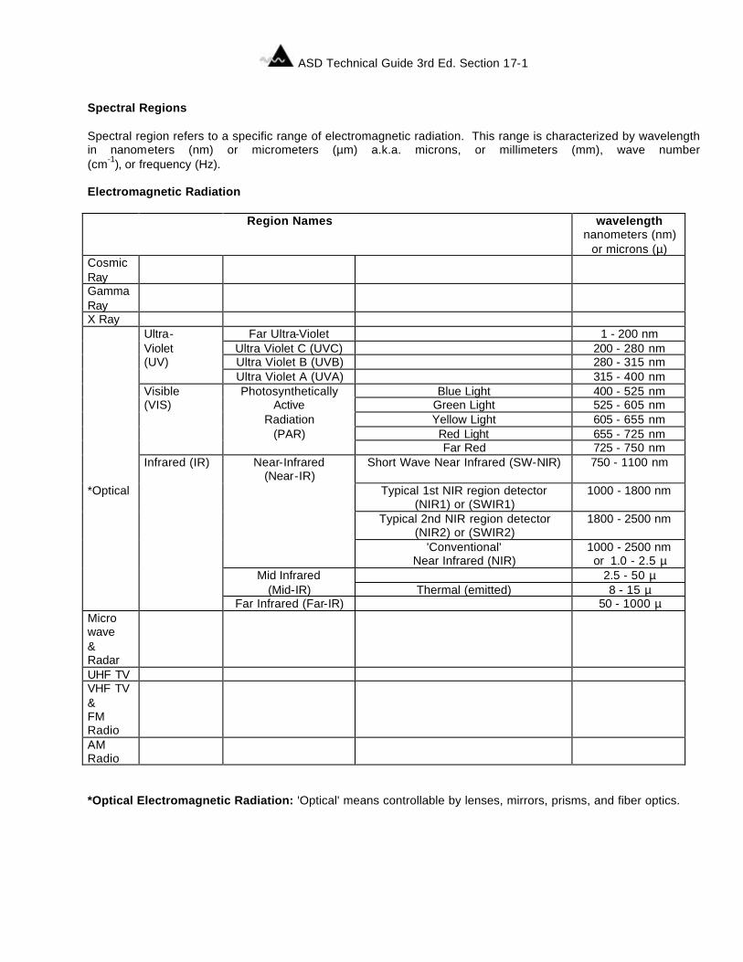
ASD Technical Guide 3rd Ed. Section 17-1
Section 17 Spectral Regions Spectral region refers to a specific range of electromagnetic radiation. This range is characterized by wavelength in nanometers (nm) or micrometers (µm) a.k.a. microns, or millimeters (mm), wave number (cm-1), or frequency (Hz). Electromagnetic Radiation Region Names wavelength
nanometers (nm) or microns (µ)
Cosmic Ray
Gamma Ray
X Ray Ultra- Far Ultra-Violet 1 - 200 nm Violet Ultra Violet C (UVC) 200 - 280 nm (UV) Ultra Violet B (UVB) 280 - 315 nm Ultra Violet A (UVA) 315 - 400 nm Visible Photosynthetically Blue Light 400 - 525 nm (VIS) Active Green Light 525 - 605 nm Radiation Yellow Light 605 - 655 nm (PAR) Red Light 655 - 725 nm Far Red 725 - 750 nm Infrared (IR) Near-Infrared
(Near-IR) Short Wave Near Infrared (SW-NIR) 750 - 1100 nm
*Optical Typical 1st NIR region detector (NIR1) or (SWIR1)
1000 - 1800 nm
Typical 2nd NIR region detector (NIR2) or (SWIR2)
1800 - 2500 nm
'Conventional' Near Infrared (NIR)
1000 - 2500 nm or 1.0 - 2.5 µ
Mid Infrared 2.5 - 50 µ (Mid-IR) Thermal (emitted) 8 - 15 µ Far Infrared (Far-IR) 50 - 1000 µ Micro wave & Radar
UHF TV VHF TV & FM Radio
AM Radio
*Optical Electromagnetic Radiation: 'Optical' means controllable by lenses, mirrors, prisms, and fiber optics.

ASD Technical Guide 3rd Ed. Section 17-2
ASD Technical Guide 3rd Ed. Section 18-1
Section 18 Reflectance by David Hatchell By definition, reflectance, R, is a calculation, such that for a given wavelength channel: R = Energy reflected from target / Energy incident on target In the case of optical radiant energy, the construction known as radiance, L, is used to quantify the optical radiant energy. Radiance has the units, Watts per square meter per steradian per nanometer (W/m2/str/nm). So, in this case, let Lt be radiance reflected from the target, and Li be radiance incident on the target. Then, for a given wavelength channel: R = Lt / Li You can see that in this calculation of R, the units (W/m2/str/nm) cancel out. So, as long as our instrument is configured to properly view Lt and Li, it really doesn't matter that it be calibrated to absolute units. All we really need is the response of the instrument for Lt in some unit of measure and the response of the instrument for Li in the same unit of measure. In the case of an analog photo detector, PD, the current produced by the PD is linear in response to radiance (voltage is approximately logarithmic). This analog current signal can be converted to digital numbers, DN, as in the FieldSpec, giving the following for a given wavelength channel: R = DNt / DNi Reference panel method for measuring reflectance: Now as far as the forementioned "properly view Lt and Li" is concerned, one can easily measure Lt by pointing the fiberoptic input of the FieldSpec at the target. But where does one point the fiberoptic to measure Li, especially in the case of outdoor measurements using solar illumination? Do you point it at the sun? Do you point it at the sky? Do you point it somewhere in the middle? In other words, how, with the limited field-of-view, FOV, of any optical input do you view all the incident energy of the sun and sky per unit steradian? The answer is to aim the fiberoptic input at a diffuse white reflectance panel (sometimes called a calibration panel) that provides a diffuse homogeneous mix of all the full sky and sun radiance reflected at nearly 100 percent up to the fiberoptic input. By the way, chemists like to call this white reference measurement the "baseline". (Ir)radiance method for measuring reflectance: A second method for measuring R involves the construction known as irradiance, E, which has units Watts per square meter per nanometer (W/m2/nm). Again, E is another way of quantifying optical radiant energy. E was also constructed to have a relationship with L. There are many good references discussing the concepts and derivations associated with E and L, such as those listed at the end of this essay. I would like to point out, that these concepts are often introduced by relating L to point emitters and E to flat receivers. While such a presentation offers one example of applying these concepts, this example is not the whole story. Without digressing to much, in general, L and E are geometric constrictions for quantifying the optical radiant energy within a space as it impinges on a geometric surface, regardless of where it came from or where it is going. Well, getting back to E, there is a relation between E and L such that in the case of solar, full-sky incident energy Ei, for a given wavelength channel: Lt = R Ei / π Therefore: R = π Lt / Ei I'm assuming the distance from the target to the fiberoptic input is close enough that atmospheric attenuation of transmission, T, is negligible. Such atmospheric effects become noticeable for great distances between target
ASD Technical Guide 3rd Ed. Section 18-2
and spectrometer, such as from a flying aircraft to the ground. I'm also neglecting stray light radiance, S, back-scattered from the atmosphere or reflected from buildings, trees or other objects too near the target. A more thorough equation for such cases would be of the form: Lt = S + RE i T / π Assuming conditions allow the simpler equation (R = π Lt / Ei) to hold, one can measure R for a given wavelength channel by measuring Lt and then attach a cosine collection device to the fiberoptic input to measure Ei. Of course, measuring R this way, does require absolute radiometric calibrations, one for radiance using the fiberoptic input, (and/or fiberoptic input with FOV) and one for irradiance using the cosine collector attached to the fiberoptic input. This second approach also offers the ability for near continuous monitoring by using two spectroradiometers. One spectroradiometer continuously monitors Ei while the other is used for Lt measurements. NOTE: Calibrated White Spectralon is a near 100% diffuse (Lambertian) reference reflectance panel made from a sintered poly - tetra - fluorethylene based material. You may also want to consider material such as Sintered Halon or Barium Sulfate (BaSO4) powder. We prefer Spectralon, which you may purchase through ASD or directly from the vender: Labsphere, Inc., Shaker St., PO Box 70, North Sutton, NH 03260-0070, PH: 603-927-4266, FX: 603-927-4694, E-mail: [email protected], Website: www.labsphere.com. References: Remote Sensing Optics and Optical Systems, by Phillip N. Slater, 1980, Addison-Wesly Publishing Company, Reading, MA Remote Sensing and Image Interpretation, by Thomas M. Lillesand and Ralph W. Kiefer, 1994, John Wiley & Sons, Inc., New York Introduction to the Physics and Techniques of Remote Sensing, by Charles Elachi, 1987, John Wiley & Sons, Inc., New York Fundamentals of Radiometry: Calculation, Measurement, and Calibration, by James M. Palmer, 1995, SPIE, Bellingham, WA "Ground Reflectance Measurement Techniques: A Comparison", by M. J. Duggin and T. Cunia, in Applied Optics, December 1993, vol 22, No. 23 "Radiance", by Fred E. Nicodemus, in American Journal of Physics, Vol. 31(5), 1963 "Distribution of Optical Radiation with Respect to Position and Direction -- Radiance", by Fred E. Nicodemus and Henry J. Kostkowski, in National Bureau of Standards Technical Notes, Vol. 910-1: 10-44, 58-59, 61, 1976
ASD Technical Guide 3rd Ed. Section 19-1
Section 19 Wavelength and Radiometric Calibration Methods
WAVELENGTH AND RADIOMETRIC CALIBRATION METHODS by Dave Beal, Analytical Spectral Devices, Inc.
Introduction: Reliable field spectrometry data collection depends, to perhaps the greatest extent, upon accurate calibration of the instruments used. The Analytical Spectral Devices FieldSpec line of spectroradiometers is commonly used in the analysis and cross-referencing of Reflectance, Transmittance, and Absorption characteristics of materials and land/sea surfaces. For this reason, accurate wavelength calibration is a necessity and a standard feature included in the acquisition of any FieldSpec instrument package. Periodic examination of the absorption features in the spectra of materials with known characteristics is highly recommended for the SWIR (short wave infrared; 1000 - 2500 nm) detectors. A mercury discharge tube or other known discrete emission light source works well for verifying calibration in the VNIR (visible and near infrared; 350 - 1000 nm) portion of the spectrum. After the instruments are calibrated at the ASD factory with a 0.1 nm bandpass monochromator, their responses to several known elements and emission sources are checked, before shipment, as a verification of method and equipment. Due to the consistency of the detector performance in the FieldSpec instruments, they are also commonly used, as their name implies, in radiometry applications. This, naturally, requires accurate and reliable radiometric calibrations for the instrument and accessories used in such applications, as well as software for manipulation of calibration and data files. Radiometric calibration is an optional feature in the purchase of any FieldSpec instrument and, in most cases, must be performed at Analytical Spectral Devices’ factory, in Boulder, CO, USA. This paper is intended as a guide for current and potential ASD customers who would like to know more about our methodology in calibration so that they can make a better informed decision about how they would like to proceed with their instruments; and perhaps even in how they would prefer to collect and analyze their data. Reflectance or Radiance? Many papers written on the subject refer to the use of spectroradiometers in field reflectance factor measurements. This is because with some instruments, it is best to use the ratio of the reflected radiance of the observed sample to the reflected radiance of a known reference panel (taken at the same time), in order to determine the reflectance factor of the sample. Of course, when this is done, all units fall out in the result, which is typically a number between zero and one for each channel measured. However, instruments such as the FieldSpec spectroradiometer, with a well-characterized linear response, can be used for the same purpose without going to the trouble and expense of radiometric calibration. Raw signal inputs from the sample and the reference panel can be ratioed to achieve the same result. This does not mean that FieldSpec instruments must be used only as spectrometers, or spectrophotometers, as the case may be. On the contrary, at least one-fourth of ASD’s customers have a true need for spectroradiometric data. Spectroradiometric needs might include: Ground-truthing of reflected radiance data collected from high altitudes or from different instruments, radiance of molten solids such as lava, steel and glass, solar irradiance at various levels of the Earth’s atmosphere and points on the Earth’s surface, studies in photosynthesis, flame studies, and synthetic light studies, among many others. But for most of our customers, who use the instruments for remote sensing ground truthing exercises, material absorptance/reflectance characteristics, water/snow/ice studies and mineral identification, an instrument with a good linear response to intensity across the spectral region of interest is all that is needed, in addition to an accurate wavelength calibration, of course. Wavelength Calibration: Wavelength calibration is a standard feature of all ASD instruments. Typically, one calibration will be accurate to within one nanometer and is guaranteed for one year. ASD will always recalibrate a FieldSpec instrument’s wavelength values once, within that time, at no extra charge. The UV/VNIR detector array and housing combine to provide a simple linear relationship between wavelength and channel number. For this reason, all that is needed for calibration is a few well-characterized emission lines, spread throughout the region from 350 - 1000 nm wavelength, and a finely focused instrument. At ASD, the emission lines come from a separate monochromator, set to emit at 50 nm intervals, which are plotted against the responding channel numbers,
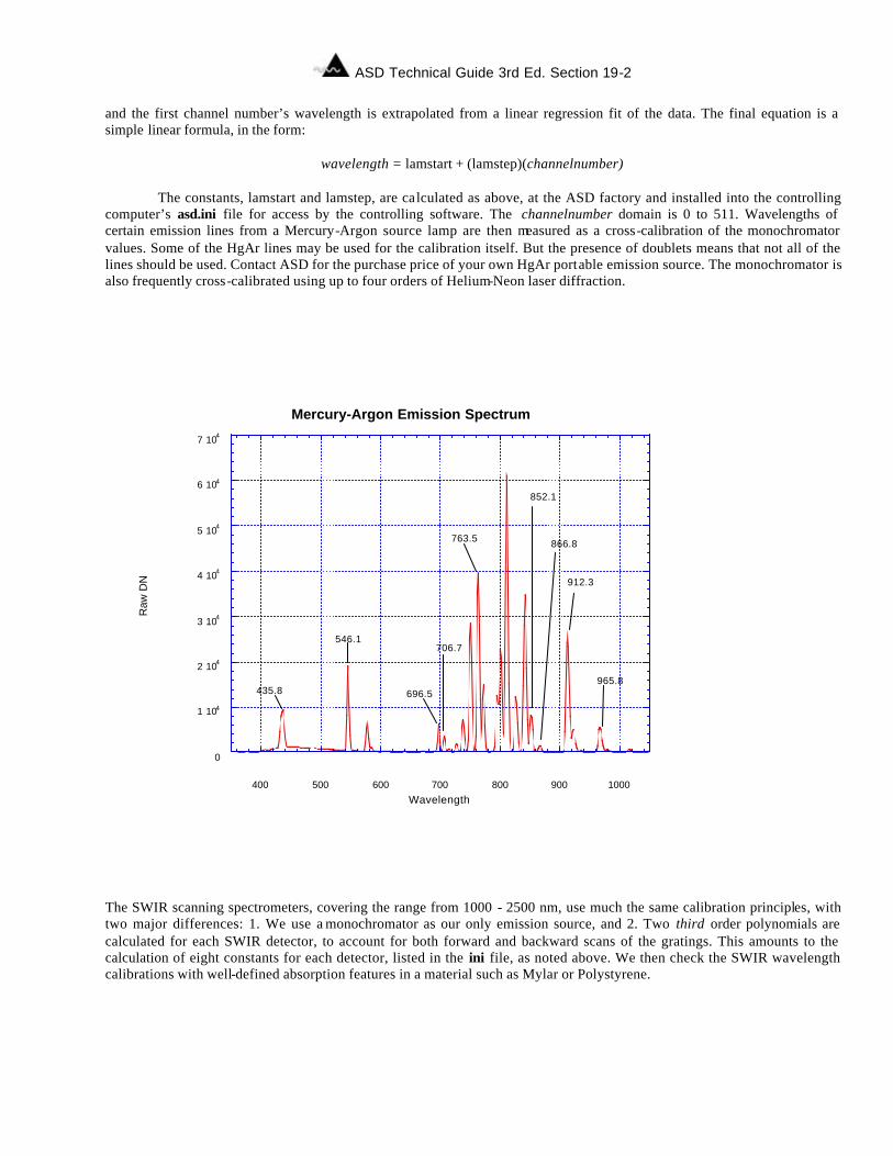
ASD Technical Guide 3rd Ed. Section 19-2
and the first channel number’s wavelength is extrapolated from a linear regression fit of the data. The final equation is a simple linear formula, in the form:
wavelength = lamstart + (lamstep)(channelnumber)
The constants, lamstart and lamstep, are calculated as above, at the ASD factory and installed into the controlling computer’s asd.ini file for access by the controlling software. The channelnumber domain is 0 to 511. Wavelengths of certain emission lines from a Mercury-Argon source lamp are then measured as a cross-calibration of the monochromator values. Some of the HgAr lines may be used for the calibration itself. But the presence of doublets means that not all of the lines should be used. Contact ASD for the purchase price of your own HgAr portable emission source. The monochromator is also frequently cross-calibrated using up to four orders of Helium-Neon laser diffraction.
0
1 104
2 104
3 104
4 104
5 104
6 104
7 104
400 500 600 700 800 900 1000
Mercury-Argon Emission Spectrum
Raw
DN
Wavelength
435.8
546.1
696.5
706.7
763.5
852.1
866.8
912.3
965.8
The SWIR scanning spectrometers, covering the range from 1000 - 2500 nm, use much the same calibration principles, with two major differences: 1. We use a monochromator as our only emission source, and 2. Two third order polynomials are calculated for each SWIR detector, to account for both forward and backward scans of the gratings. This amounts to the calculation of eight constants for each detector, listed in the ini file, as noted above. We then check the SWIR wavelength calibrations with well-defined absorption features in a material such as Mylar or Polystyrene.
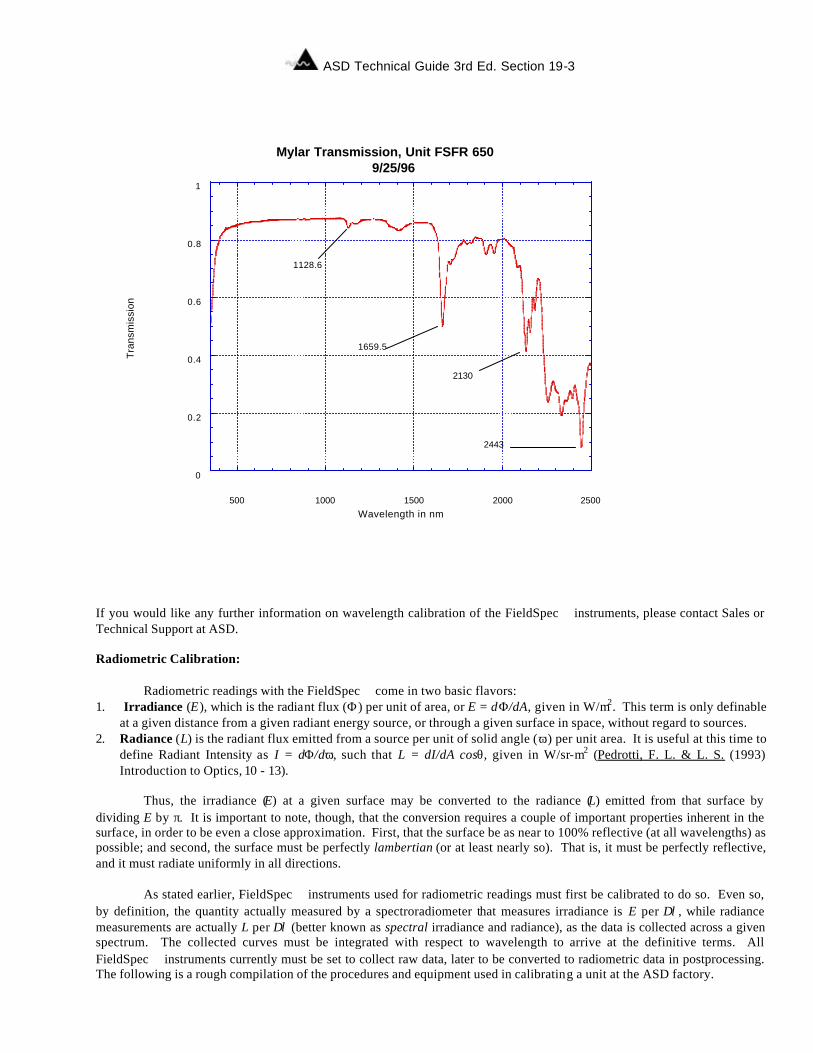
ASD Technical Guide 3rd Ed. Section 19-3
0
0.2
0.4
0.6
0.8
1
500 1000 1500 2000 2500
Mylar Transmission, Unit FSFR 6509/25/96
Tra
nsm
issi
on
Wavelength in nm
1128.6
1659.5
2130
2443
If you would like any further information on wavelength calibration of the FieldSpec instruments, please contact Sales or Technical Support at ASD. Radiometric Calibration: Radiometric readings with the FieldSpec come in two basic flavors: 1. Irradiance (E), which is the radiant flux (Φ) per unit of area, or E = dΦ/dA, given in W/m2. This term is only definable
at a given distance from a given radiant energy source, or through a given surface in space, without regard to sources. 2. Radiance (L) is the radiant flux emitted from a source per unit of solid angle (ω) per unit area. It is useful at this time to
define Radiant Intensity as I = dΦ/dω, such that L = dI/dA cosθ, given in W/sr-m2 (Pedrotti, F. L. & L. S. (1993) Introduction to Optics, 10 - 13).
Thus, the irradiance (E) at a given surface may be converted to the radiance (L) emitted from that surface by
dividing E by π. It is important to note, though, that the conversion requires a couple of important properties inherent in the surface, in order to be even a close approximation. First, that the surface be as near to 100% reflective (at all wavelengths) as possible; and second, the surface must be perfectly lambertian (or at least nearly so). That is, it must be perfectly reflective, and it must radiate uniformly in all directions. As stated earlier, FieldSpec instruments used for radiometric readings must first be calibrated to do so. Even so, by definition, the quantity actually measured by a spectroradiometer that measures irradiance is E per ∆λ, while radiance measurements are actually L per ∆λ (better known as spectral irradiance and radiance), as the data is collected across a given spectrum. The collected curves must be integrated with respect to wavelength to arrive at the definitive terms. All FieldSpec instruments currently must be set to collect raw data, later to be converted to radiometric data in postprocessing. The following is a rough compilation of the procedures and equipment used in calibrating a unit at the ASD factory.
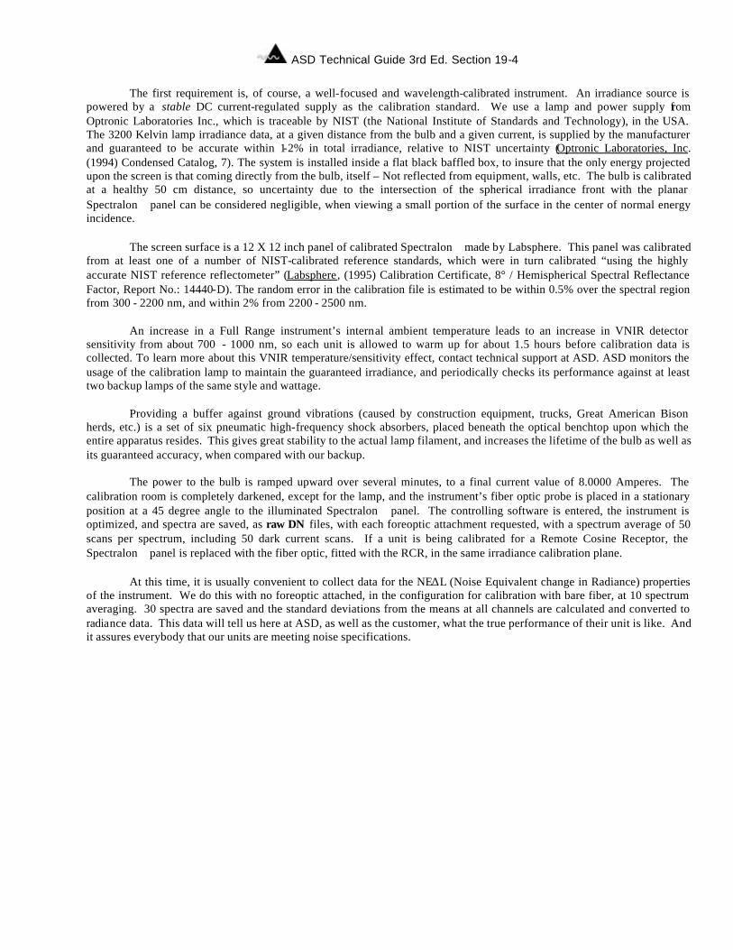
ASD Technical Guide 3rd Ed. Section 19-4
The first requirement is, of course, a well-focused and wavelength-calibrated instrument. An irradiance source is powered by a stable DC current-regulated supply as the calibration standard. We use a lamp and power supply from Optronic Laboratories Inc., which is traceable by NIST (the National Institute of Standards and Technology), in the USA. The 3200 Kelvin lamp irradiance data, at a given distance from the bulb and a given current, is supplied by the manufacturer and guaranteed to be accurate within 1-2% in total irradiance, relative to NIST uncertainty (Optronic Laboratories, Inc. (1994) Condensed Catalog, 7). The system is installed inside a flat black baffled box, to insure that the only energy projected upon the screen is that coming directly from the bulb, itself – Not reflected from equipment, walls, etc. The bulb is calibrated at a healthy 50 cm distance, so uncertainty due to the intersection of the spherical irradiance front with the planar Spectralon panel can be considered negligible, when viewing a small portion of the surface in the center of normal energy incidence. The screen surface is a 12 X 12 inch panel of calibrated Spectralon made by Labsphere. This panel was calibrated from at least one of a number of NIST-calibrated reference standards, which were in turn calibrated “using the highly accurate NIST reference reflectometer” (Labsphere, (1995) Calibration Certificate, 8° / Hemispherical Spectral Reflectance Factor, Report No.: 14440-D). The random error in the calibration file is estimated to be within 0.5% over the spectral region from 300 - 2200 nm, and within 2% from 2200 - 2500 nm. An increase in a Full Range instrument’s internal ambient temperature leads to an increase in VNIR detector sensitivity from about 700 - 1000 nm, so each unit is allowed to warm up for about 1.5 hours before calibration data is collected. To learn more about this VNIR temperature/sensitivity effect, contact technical support at ASD. ASD monitors the usage of the calibration lamp to maintain the guaranteed irradiance, and periodically checks its performance against at least two backup lamps of the same style and wattage. Providing a buffer against ground vibrations (caused by construction equipment, trucks, Great American Bison herds, etc.) is a set of six pneumatic high-frequency shock absorbers, placed beneath the optical benchtop upon which the entire apparatus resides. This gives great stability to the actual lamp filament, and increases the lifetime of the bulb as well as its guaranteed accuracy, when compared with our backup. The power to the bulb is ramped upward over several minutes, to a final current value of 8.0000 Amperes. The calibration room is completely darkened, except for the lamp, and the instrument’s fiber optic probe is placed in a stationary position at a 45 degree angle to the illuminated Spectralon panel. The controlling software is entered, the instrument is optimized, and spectra are saved, as raw DN files, with each foreoptic attachment requested, with a spectrum average of 50 scans per spectrum, including 50 dark current scans. If a unit is being calibrated for a Remote Cosine Receptor, the Spectralon panel is replaced with the fiber optic, fitted with the RCR, in the same irradiance calibration plane.
At this time, it is usually convenient to collect data for the NE∆L (Noise Equivalent change in Radiance) properties of the instrument. We do this with no foreoptic attached, in the configuration for calibration with bare fiber, at 10 spectrum averaging. 30 spectra are saved and the standard deviations from the means at all channels are calculated and converted to radiance data. This data will tell us here at ASD, as well as the customer, what the true performance of their unit is like. And it assures everybody that our units are meeting noise specifications.
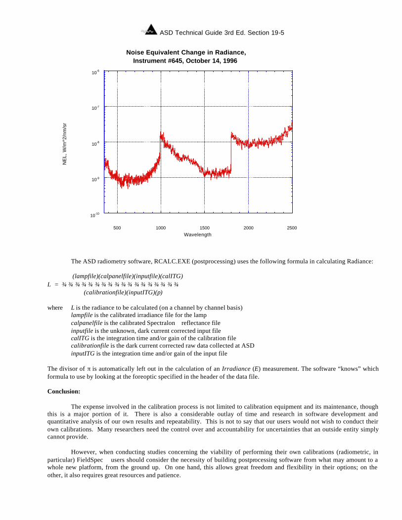
ASD Technical Guide 3rd Ed. Section 19-5
10-10
10-9
10-8
10-7
10-6
500 1000 1500 2000 2500
Noise Equivalent Change in Radiance,Instrument #645, October 14, 1996
NE
L, W
/m^2
/nm
/sr
Wavelength
The ASD radiometry software, RCALC.EXE (postprocessing) uses the following formula in calculating Radiance:
(lampfile)(calpanelfile)(inputfile)(calITG)
L = (calibrationfile)(inputITG)(π) where L is the radiance to be calculated (on a channel by channel basis) lampfile is the calibrated irradiance file for the lamp calpanelfile is the calibrated Spectralon reflectance file inputfile is the unknown, dark current corrected input file calITG is the integration time and/or gain of the calibration file calibrationfile is the dark current corrected raw data collected at ASD inputITG is the integration time and/or gain of the input file The divisor of π is automatically left out in the calculation of an Irradiance (E) measurement. The software “knows” which formula to use by looking at the foreoptic specified in the header of the data file. Conclusion:
The expense involved in the calibration process is not limited to calibration equipment and its maintenance, though this is a major portion of it. There is also a considerable outlay of time and research in software development and quantitative analysis of our own results and repeatability. This is not to say that our users would not wish to conduct their own calibrations. Many researchers need the control over and accountability for uncertainties that an outside entity simply cannot provide. However, when conducting studies concerning the viability of performing their own calibrations (radiometric, in particular) FieldSpec users should consider the necessity of building postprocessing software from what may amount to a whole new platform, from the ground up. On one hand, this allows great freedom and flexibility in their options; on the other, it also requires great resources and patience.

ASD Technical Guide 3rd Ed. Section 19-6
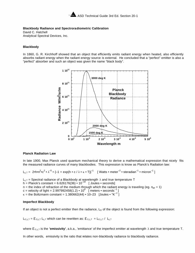
ASD Technical Guide 3rd Ed. Section 20-1
Section 20 Blackbody Radiance and Spectroradiometric Calibration David C. Hatchell Analytical Spectral Devices, Inc. Blackbody In 1860, G. R. Kirchhoff showed that an object that efficiently emits radiant energy when heated, also efficiently absorbs radiant energy when the radiant energy source is external. He concluded that a “perfect” emitter is also a “perfect” absorber and such an object was given the name “black body”. Planck Radiation Law In late 1900, Max Planck used quantum mechanical theory to derive a mathematical expression that nicely fits the measured radiance curves of many blackbodies. This expression is know as Planck’s Radiation law: Lλ,T = 2•h•n2•c2 • λ–5 • –1 + exp(h • c / λ • κ • T)–1 [ Watts • meter–2 • steradian–1 • micron–1 ] Lλ,T = Spectral radiance of a Blackbody at wavelength λ and true temperature T h = Planck’s constant = 6.626176(36) • 10–34 [ Joules • seconds] n = the index of refraction of the medium through which the radiant energy is traveling (eg. nair = 1) c = velocity of light = 2.997992458(1.2) • 108 [ meters • seconds–1 ] κ = the Boltzmann constant = 1.380662(44) • 10–23 [Joules • °K–1 ] Imperfect Blackbody If an object is not a perfect emitter then the radiance, LO of the object is found from the following expression:
LO,λ,T = εO,λ,T Lλ,T which can be rewritten as: εO,λ,T = LO,λ,T / Lλ,T
where εO,λ,T is the 'emissivity', a.k.a., 'emittance' of the imperfect emitter at wavelength λ and true temperature T. In other words, emissivity is the ratio that relates non-blackbody radiance to blackbody radiance.
0
2 1011
4 1011
6 1011
8 1011
1 1012
0 100 1 10-6 2 10-6 3 10-6 4 10-6 5 10-6
Rad
ian
ce W
/m2 /s
r/m
Wavelength m
3000 deg K
2000 deg K
1500 deg K
PlanckBlackbody Radiance
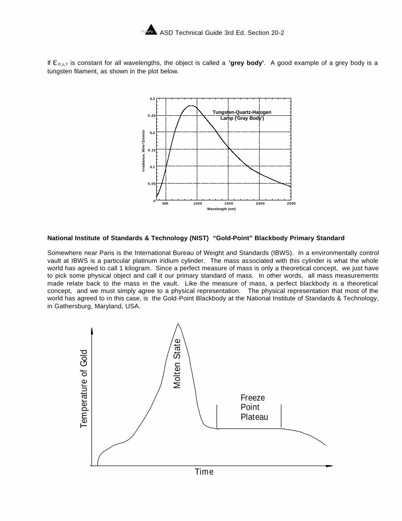
ASD Technical Guide 3rd Ed. Section 20-2
If εO,λ,T is constant for all wavelengths, the object is called a 'grey body'. A good example of a grey body is a tungsten filament, as shown in the plot below. National Institute of Standards & Technology (NIST) “Gold-Point” Blackbody Primary Standard Somewhere near Paris is the International Bureau of Weight and Standards (IBWS). In a environmentally control vault at IBWS is a particular platinum iridium cylinder. The mass associated with this cylinder is what the whole world has agreed to call 1 kilogram. Since a perfect measure of mass is only a theoretical concept, we just have to pick some physical object and call it our primary standard of mass. In other words, all mass measurements made relate back to the mass in the vault. Like the measure of mass, a perfect blackbody is a theoretical concept, and we must simply agree to a physical representation. The physical representation that most of the world has agreed to in this case, is the Gold-Point Blackbody at the National Institute of Standards & Technology, in Gathersburg, Maryland, USA.
0
0.05
0.1
0.15
0.2
0.25
0.3
500 1000 1500 2000 2500
Tungsten-Quartz-HalogenLamp ('Gray Body')
Irra
dia
nce
, W/m
^2/n
m/s
r
Wavelength (nm)
Time
Tem
pera
ture
of G
old
Mol
ten
Stat
e
FreezePointPlateau
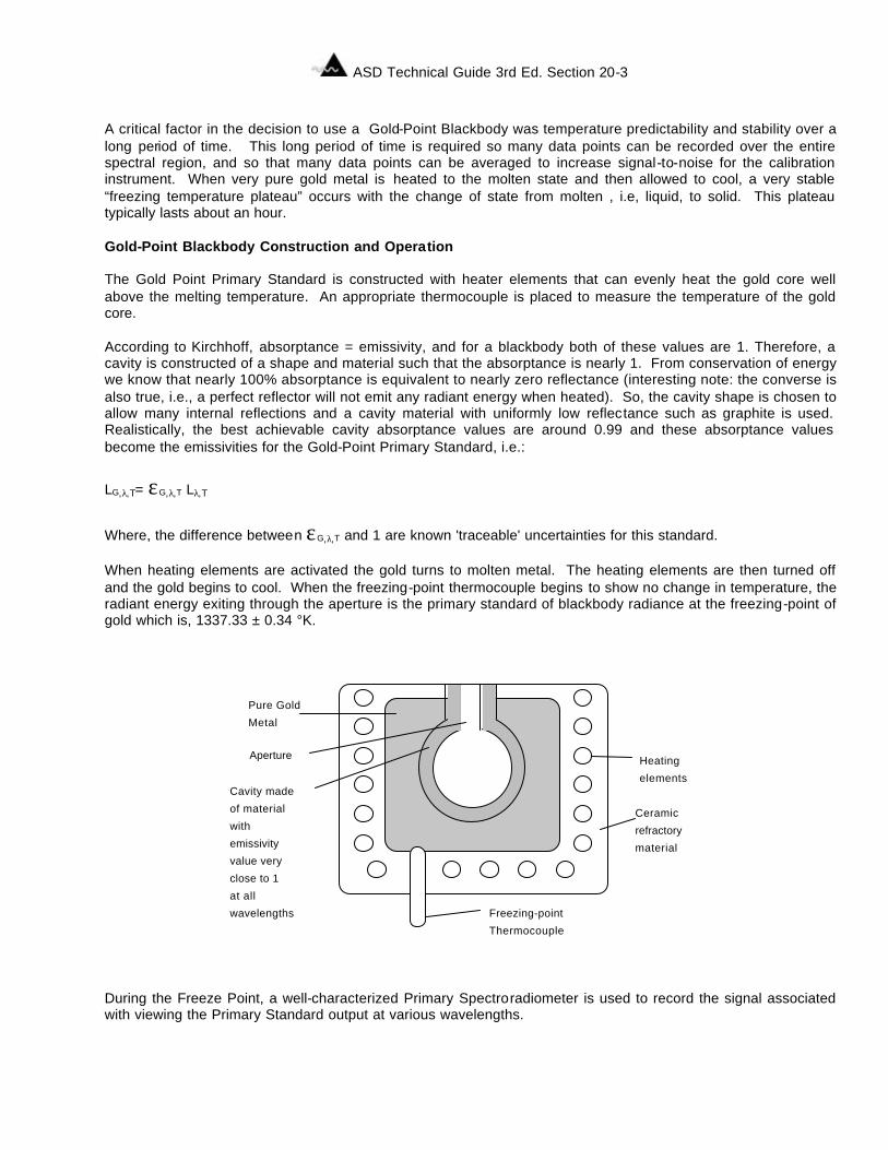
ASD Technical Guide 3rd Ed. Section 20-3
A critical factor in the decision to use a Gold-Point Blackbody was temperature predictability and stability over a long period of time. This long period of time is required so many data points can be recorded over the entire spectral region, and so that many data points can be averaged to increase signal-to-noise for the calibration instrument. When very pure gold metal is heated to the molten state and then allowed to cool, a very stable “freezing temperature plateau” occurs with the change of state from molten , i.e, liquid, to solid. This plateau typically lasts about an hour. Gold-Point Blackbody Construction and Operation The Gold Point Primary Standard is constructed with heater elements that can evenly heat the gold core well above the melting temperature. An appropriate thermocouple is placed to measure the temperature of the gold core. According to Kirchhoff, absorptance = emissivity, and for a blackbody both of these values are 1. Therefore, a cavity is constructed of a shape and material such that the absorptance is nearly 1. From conservation of energy we know that nearly 100% absorptance is equivalent to nearly zero reflectance (interesting note: the converse is also true, i.e., a perfect reflector will not emit any radiant energy when heated). So, the cavity shape is chosen to allow many internal reflections and a cavity material with uniformly low reflectance such as graphite is used. Realistically, the best achievable cavity absorptance values are around 0.99 and these absorptance values become the emissivities for the Gold-Point Primary Standard, i.e.:
LG,λ,T= εG,λ,T Lλ,T
Where, the difference between εG,λ,T and 1 are known 'traceable' uncertainties for this standard. When heating elements are activated the gold turns to molten metal. The heating elements are then turned off and the gold begins to cool. When the freezing-point thermocouple begins to show no change in temperature, the radiant energy exiting through the aperture is the primary standard of blackbody radiance at the freezing-point of gold which is, 1337.33 ± 0.34 °K.
Heatingelements
Ceramicrefractorymaterial
Pure GoldMetal
Cavity madeof materialwithemissivityvalue veryclose to 1 at allwavelengths
Aperture
Freezing-pointThermocouple
During the Freeze Point, a well-characterized Primary Spectroradiometer is used to record the signal associated with viewing the Primary Standard output at various wavelengths.
ASD Technical Guide 3rd Ed. Section 20-4
Other Primary Standards Other Primary Freeze Point standards are also used to add more calibration points to the Primary Spectroradiometer. These include: Silver, freeze point 1234.93 °K Copper, freeze point 1357.77 °K Zinc, freeze point 419.58 °C Tin, freeze point 231.9681 °C Lead, freeze point 327.502 °C Appropriate interpolation functions are then used to complete the radiance response characterization of the Primary Spectroradiometer. This characterization model is recalled to characterize other 'non-Primary' standards. Lamp Transfer Standards Using the Primary Spectroradiometer, its radiance response characterization model, and an appropriate integrating sphere, the radiance of secondary 'Lamp Transfer Standards' are measured at a specific current settings. The lamp, radiance data file, current and distance settings, and traceable uncertainty numbers are sold as a package so that other similarly constructed, third level, 'Working Lamp Standards' can be calibrated. Calibration of Commercial Spectroradiometer The Working Lamp Standards, and their calibration files are used to calibrate commercial spectroradiometers. Since the radiance output of the lamps is know for the specified current and distance, the correction factors for the spectroradiometer signal output can be determined, to within the traceable uncertainties. References Klaus D. Mielenz, Robert D. Saunders, Albert C. Parr, and Jack J. Hsia, The 1990 NIST Scales of Thermal Radiometry, Journal of Research of the National Institute of Standards and Technology, Volume 95, Number 6, November-December 1990. T. P. Merritt and F. F. Hall, Jr., Blackbody Radiation, Selected Papers on Radiometry, SPIE Milestone Series, Volum MS14, Page598-604, Reprinted from Proceedings of the IRE, Vol. 47(2), 1435-1441 (1959). Arthur J. Cussen, Overview of blackbody radiation sources, SPIE Milestone Series, Volum MS14, Page 647-660, Reprinted from Infrared Sensor Technology, Proc, SPIE 344, 2-15, (1982). J.C. Richmond and D. P. DeWitt, Applications of Radiation Thermometry, A symposium sponsored by ASTM Committee E-20 on Temperature Measurement in cooperation with the National Bureau of Standards, pages 4-7, (1984).
ASD Technical Guide 3rd Ed. Section 21-1
Section 21 The Benifits of Portable NIR Analysis Portable NIR analysis is a new concept that has been made possible through advances in solid state and optical materials as well as computer miniaturization. Because portable NIR analysis is a new concept, its time and labor saving potential are limited only by the imagination of the user. But bench-top systems require that the sample be carried to the lab and carefully prepared for examination. The lab instrument performs its own sequence of steps that can take several minutes. Finally, the lab results must be communicated to the appropriate personnel. Such a procedure requires the time and effort of several persons, and may also require undesirable handling and disposal of materials. In contrast, a Portable NIR analyzer can be transported to the site of interest and measurements taken very quickly. NIR SPECTRUM The near infrared region is immediately adjacent to the visible range and falls between 750 and 3,000 nanometers in wavelength. Most organic materials have excellent reflectance or transmittance properties at these wavelengths. The biggest advantage of NIR over Mid-IR and Far-IR is sample preparation. Little or no sample preparation is required for NIR. However, significant preparation required for Mid-IR and Far-IR. For example, due to the extremely high absorption coefficients of materials in the Mid-IR and Far-IR, transmission measurements require that samples be extremely thin, including liquid samples. The samples must be placed between cell window materials that are transparent in the IR, e.g., KBr, CsBr, AgCl, and NaCl, which must be cleaved and polished. These materials are very hygroscopic and must be stored in a desiccator. 'Mulling agents' such as mineral oil must also be used in preparing solid samples. The solid sample, as a fine powder, is suspended in the mineral oil and then smeared between two cell plates. Extreme care must be taken in handling and cleaning the cells. Any oils on one's hands could contaminate the cells. Another advantage of NIR over Mid-IR and Far-IR is 'thermal' noise. All internal electronic components are a source of thermal noise in the Mid-IR and Far-IR. However, internal sources of IR are either insignificant to NIR detectors or can be made insignificant by minor shielding. The disadvantage of NIR analysis is that most of the useful features in a spectrum consist of 'overtones' or combinations of overtones, which are much subtler than the distinct fundamentals found in Mid-IR and Far-IR spectra. However, recent developments in off-the-shelf chemometrics software and powerful PC's have made NIR analysis the practical choice for most applications. SPECTRAL FEATURES According to the principles of quantum physics, molecules may only assume discrete energy levels. Similar to the vibrating string of a musical instrument, the vibration of a molecule has a fundamental frequency, i.e., wavelength as well as a series of overtones. For molecules, the fundamental vibrations involve no change in center of gravity of the molecule. The spectrum shape for any material is the result of these characteristic fundamentals and overtones. There are many fundamentals in the mid and far infrared regions. Near-infrared spectra are mainly the result of overtones. Since the molecular structure of most compounds is very complex, the resulting spectra are actually the result of many overlapping peaks and valleys. Generally speaking, persons performing NIR analysis must then identify and characterize specific features in the spectra by means of statistical methods. Chemometrics software is designed to accomplish this task. CHEMOMETRICS MODELS
ASD Technical Guide 3rd Ed. Section 21-2
In order for any NIR analyzer to make quantitative measurements or qualitative discriminations, the controlling computer must have access to one or more chemometrics models, which represent the type of material being tested. The model is a mathematical construct that had been developed using samples of the same product or class of products. The controlling computer applies the model(s) to the target spectrum and returns a model result. A chemometrics model is developed by collecting spectral readings from a group of samples that display (A) the maximum variability of the characteristic of interest, and (B) non-correlating or random variability in all other characteristics. The same samples are submitted for independent testing to measure the characteristic of interest by a standard analytical method. The spectral data and independent test data are then analyzed using commercially available chemometrics software. The statistical processes used in quantitative spectral analysis include multiple linear regression, classical least squares, inverse least squares and principal component regression. The statistical processes used in qualitative spectral analysis include K-nearest neighbors, SIMCA and others. When a sufficient number of samples has been collected and properly analyzed, a mathematical model is constructed that describes the relationship between specific spectral features and the sample characteristic of interest. Thereafter, a chemist or technician may quickly measure that same characteristic in a new target sample by applying the chemometrics model to the spectrum of the target sample. An NIR analyzer is also able to identify an unknown target sample if its spectral signature matches any of the models already developed. ASD LABSPEC PRO The LabSpec Pro is a highly portable, general-purpose spectrophotometer that has many applications for product analysis. The instrument measures the unique pattern that light reflects off or is transmitted through a product sample. The LabSpec Pro uses a fiber-optic sampling probe to deliver illumination to the physical sample and to collect reflected or transmitted light from the sample. A tungsten-halogen bulb provides the source light, which is carried by one optical fiber or bundle of fibers to the tip of the probe. A separate optical fiber carries the reflected or transmitted light back to the instrument where it passes through the entrance slit of the spectrometer. The heart of the LabSpec Pro is its proprietary spectrometer, which depending upon the model measures incoming light in the Visible (VIS), and/or near-infrared (NIR) region of the electromagnetic spectrum (see price list for different models according to spectral coverage). The instrument functions well with many available reflectance, transmission or trans-reflectance fiber-optic probes. Generally, reflectance probes are used for solids, trans-reflectance probes are used for clear liquids and transmittance probes are used for liquids containing particulates. ASD consultants can assist in the selection of appropriate fiber-optic probes for specific applications. BUILT-IN LIGHT SOURCE NIR analysis requires an adequate level of incident light on the sample. The LabSpec Pro provides a controlled source of incident light having a color temperature of 3,000°K. Even though the built-in light source is designed for stability and accuracy, characteristics of the light source are eliminated when the baseline spectrum is automatically applied to each raw sample spectrum. The internal light source reaches maximum stability after approximately 5 minutes of warm-up time. If it is necessary to acquire spectra during this warm-up period, take a new baseline spectrum immediately before taking each sample spectrum.
ASD Technical Guide 3rd Ed. Section 22-1
Section 22 Making an NIR Analyzer Work For You
MAKING AN NIR ANALYZER WORK FOR YOU
Zhao Lu, Analytical Chemist Analytical Spectral Devices, Inc.
Boulder, CO 80301 USA
ABSTRACT In recent years, NIR analysis has steadily grown in popularity because of its ability to quickly provide qualitative and quantitative information on many products, especially raw materials. To determine if NIR spectroscopy is a reasonable alternative to more traditional methods, many factors must be considered. These factors include sample characteristics, experiment configuration, and data analysis.
SAMPLE CONSIDERATION The chemical constituents and physical phenomena of interest should have direct or indirect absorbance in the NIR region. Virtually all organic compounds do, particularly those with functional groups like hydroxyl, carboxyl, amine and carbon-hydrogen. A good reference for researching near infrared spectra is The Atlas of Near Infrared Spectra, Bio-Rad Sadtler Division, Philadelphia, Pennsylvania. For calibration samples, the amount of analyte in the sample set should be above the detection limit and have sufficient variability. Some analytes are reportedly detectable at the ppm level. For most analytes, the nominal detection limit will be 1% or above. The analytical chemist must have an accurate independent method for measurement of the properties and must know the level of error in the reference methods. Errors in NIR prediction most often arise from errors in the reference methods, instability of the NIR spectrometer, and inappropriate choice of the calibration model. The samples used in the development of calibration sets must be representative. All the variations in the future unknown samples should be covered in the "training" calibration sets, for example, sample composition and particle size, homogeneity, and temperature variation at the working environment. As a rule of thumb, the more samples you have for the training set, the more reliable the calibration model.
EXPERIMENT CONFIGURATION When using an NIR analyzer, instrument characteristics such as sensitivity, resolution, and signal-to-noise ratio parameters need to be evaluated. The quality of these values is a function of the light source stability, optics throughput, dispersion/filter element accuracy, and detector sensitivity in the instrument. The choice of accessories is application dependent. For liquid samples, transmission and transflectance modes are commonly employed using fiber optic probes or cuvettes. The path length is sample dependent, usually ranging from 0.1 to 1 cm. The advantage of using a fiber-optic probe is that sample preparation is significantly reduced and noninvasive or nondestructive measurements become possible. For solid samples, diffuse-reflectance spectra collected by a reflectance probe will provide information for analytes. Diffuse reflectance should be measured without interference from specular reflectance. The setup configuration, such as the angle of incident light and the distance of light illumination / collection ought to be consistent through all the measurements, including those taken in developing the calibration set and for predicting the future unknowns. For solid samples, the sample should be rotated and measurements done on different spots of the sample to average out the sampling error. A group of spectra may be averaged to increase the signal-to-noise ratio.
ASD Technical Guide 3rd Ed. Section 22-2
Random noise is reduced by the factor, square root of the number of spectra averaged. For ASD’s portable NIR spectrometer, it takes 0.1 seconds to acquire one spectrum. Therefore, a 10 second measurement reduces the random noise by a factor of 10.
DATA ANALYSIS NIR spectroscopy is an extremely rapid method of measurement, capable of performing an analysis within a minute. The time-consuming part of NIR work is the data analysis phase, where chemists try to find the correlation between near-infrared spectral characteristics and the property, or properties, of interest as measured by more traditional methods. There are several commercially available software packages for doing this task. Data analysis involves the following steps. Data preprocessing: When the spectral data plots are presented, first determine if there is any baseline drift or slope in the spectra, which often occurs in diffuse-reflectance measurements. Baseline subtraction, first derivative and second derivative transformations may be performed to reduce these effects if necessary. There is a trade-off though, each successive degree of derivative that is taken introduces more noise into the spectral data. Outlier detection: An outlier is a data point that falls well outside of the main population. Outliers result from lab measurement errors, samples from different categories, and instrument error. It is important to check for and remove outliers in both the training set and the set of unknowns that the calibration is to be tested on (see "validation" and "prediction"). Building a good calibration model: This is one of the most important steps in NIR analysis. Developing a calibration model involves calculating the regression equation based on the NIR spectra and the known analyte information. The model is then used to predict the future unknowns. Multiple Linear Regression (MLR), Principal Component Regression (PCR) and Partial Least Squares (PLS) are commonly used linear calibration methods, along with Locally Weighted Regression (LWR) for nonlinear models. In developing a calibration model, several parameters are evaluated: factors, loadings, and scores. When choosing the number of factors, one should try to avoid under-fitting, i.e. too few factors, and over-fitting, i.e. too many factors. If an insufficient number of factors are chosen, the prediction is not reliable because useful information has been left out. If too many factors are chosen, however, more uncertainty is included in the calibration set which will result in errors in prediction. Scores are used to check the sample homogeneity and possible clusters, while loadings are used to interpret how the variables are weighted in principal component space. Validation: The validity of the model must be tested. Usually the way this is done is to split the whole sample set into two sets; one set for calibration and the other for validation. If there are not enough samples, “leave-one-out” cross validation can be performed. This means leaving one sample out, using the rest of the samples to build a calibration model and then using the model to predict the one that was left out. The advantage of doing cross validation is that, unlike calibration with a full data set, the sample being predicted is not included in the calibration model. Thus, the model can be tested independently. Prediction:
Finally, the calibration can be used to predict future unknowns, assuming that the unknowns are in the same sample population as those used in the calibration set. Whether the unknown is an outlier needs to be tested.
SUMMARY Applying an NIR analyzer to a particular application requires the development of a reliable calibration model. The most important steps involve a thorough consideration of experimental design and multivariate calibration. Once this is established, one can enjoy the advantages of the NIR analysis. The speed of the analysis will save time and avoid many mistakes instantaneously. The speed advantage is so valuable to engineers involved with
ASD Technical Guide 3rd Ed. Section 22-3
on-line process monitoring that instruments are routinely installed in the process line with feedback loops. With a portable NIR analyzer such as the LabSpec® Pro spectrometer, samples can be noninvasively analyzed on-the-spot, dramatically reducing costly and time consuming laboratory analysis. The low absorptivity in the NIR region allows measurements to be taken on raw materials without elaborate sample preparation. In the food, agriculture, pharmaceutical, polymer, cosmetics, environmental, textile, and medical fields , portable NIR analysis finds a wide range of applications. There are still many unknown applications waiting to be discovered and with the maturity of this technique, more and more people will use portable NIR analyzers for convenience and flexibility.
REFERENCES Burns D. A. and E. W. Ciurczak (Eds.), Handbook of Near-Infrared Analysis, (Volume 13 in Practical Spectroscopy Series), Marcel Dekker, Inc., New York, 1992 Hildrum K. I., T. Isaksson, T. Naes and A. Tandberg (Eds.), Near Infra-red Spectroscopy, (Ellis Horwood Series in Analytical Chemistry), Ellis Horwood, Ltd., England, 1992 Murray I. and I. A. Cowe (Eds.), Making Light Work: Advances in Near Infrared Spectroscopy, 4th International Conference on Near Infrared Spectroscopy, Aberdeen, Scotland, August 19-23, 1991, Weinheim, New York, Basel, Cambridge, VCH, 1992

ASD Technical Guide 3rd Ed. Section 22-4
ASD Technical Guide 3rd Ed. Section 23-1
Section 23 Derivation of Bouguer-Lambert-Beer (BLB) Law
Derivation of Bouguer-Lambert-Beer (BLB) Law David Hatchell, ASD
Bouguer-Lambert-Beer Law (BLB): The most useful concept in spectrophotometry is the Bouguer-Lambert-Beer Law (BLB). When reflection, fluorescence, and Raman scattering are negligible BLB works very well to determine the concentration of absorbing species in dilute solutions. Another important condition is that the source be monochromatic (same wavelength) or all measurements must be made as a function of wavelength4. Omitting the wavelength nomenclature for clarity, BLB is derived as follows: Let N equal the total number of photons for one second striking a sample of thickness x and a defined surface area of one square centimeter. For the infinitesimal thickness element dx there is an associated decrease –dN in the number of photons allowed to pass through to the next infinitesimal thickness element. This decrease is caused by absorption and it must be proportional to the total number N for thickness x . Therefore:
- dNdx
∝ Nx
Now since x is partially determined by the number of molecules m in the sample, x must be proportional to the total number
of molecules. That is 1x
∝ m . Letting the constant of proportionality = k gives, 1x
= kcm Letting k also absorb the
constant of proportionality for - dNdx
∝ Nx
gives:
- dNdx
= kmN
Since the intensity I of a flux component is in part determined by the number of photons, I must be proportional to N and dI must be proportional to dN . Therefore, Letting k also absorb this constant of proportionality gives:
- dIdx
= km I
This equation can then be rewritten in integral form as follows:
- ⌡⌠
Io
Iι
dI I
= km ⌡⌠0
ι
dx
where ι is the total length of the path length traversed by the transmitted flux and Io is the intensity of the source flux, and
Iι is the intensity of the transmitted flux after passing through the matter. If the incident flux Fo is collimated, that is, all incident flux lines are parallel, and if it is normal to the sample surface, the path length is simply a straight line, giving:
- ln IιIo
= kmι , which can be rewritten as: ln IοIι
= kmι
Letting K = km
ln10 , gives (see note5):
4Gordon Marc Loudon, "The Necessity of Using Monochromatic Radiation in Spectrometry", Journal of Chemical Education, v. 41 (July 1964), p. 391.
5 "natural log" = loge = ln, the factor 1
ln10 converts "ln" to "log10" hereafter "log"
ASD Technical Guide 3rd Ed. Section 23-2
log IοIι
= Kι which is the Bouguer-Lambert part of BLB.
Absorbance (Abs): The quantity, log IοIι
is known as the 'absorbance'. Experiment also shows that absorbance is
proportional to the concentration c of the absorbing species. Letting the proportionality constant be α gives the experimental result of: Abs = αc which is Beer's contribution to the Bouguer-Lambert-Beer law. Beer's and Bouguer-Lambert can be combined via the total differential to form the combined BLB law (see Lohman for the combined derivation)6: Abs = αλιc
where αλ is called the molar absorption coefficient and has units of liters per mole per centimeter. The λ subscript indicates
the wavelength dependence of molar absorption coefficient. When referring to the sphectrophotometric Bouguer-Lambert type measurement the units are usually indicated by AU for absorbance units (eg. absorbance = 6 AU). Abs is used when referring to Beer's expression.
6Fred H. Lohman, "The Mathematical Combination of Lambert's Lw and Beer's Law", Journal of Chemical Education, v. 32 (March 1955), p. 155.
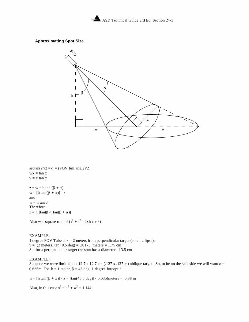
ASD Technical Guide 3rd Ed. Section 24-1
Section 24
Approximating Spot Size
α
x
y
FOV
z
βh
w
arctan(y/x) = α = (FOV full angle)/2 y/x = tan α y = x tan α z + w = h tan (β + α) w = [h tan (β + α)] - z and w = h tan β Therefore: z = h [tan(β)+ tan(β + α)] Also w = square root of (x2 + h2 - 2xh cosβ) EXAMPLE: 1 degree FOV Tube at x = 2 meters from perpendicular target (small ellipse): y = (2 meters) tan (0.5 deg) = 0.0175 meters = 1.75 cm So, for a perpendicular target the spot has a diameter of 3.5 cm EXAMPLE: Suppose we were limited to a 12.7 x 12.7 cm (.127 x .127 m) oblique target. So, to be on the safe side we will want z = 0.635m. For h = 1 meter, β = 45 deg, 1 degree foreoptic: w = [h tan (β + α)] - z = [tan(45.5 deg)] - 0.635]meters = 0.38 m Also, in this case x2 = h2 + w2 = 1.144

ASD Technical Guide 3rd Ed. Section 24-2
ASD Technical Guide 3rd Ed. Section 25-1
Section 25 Foliar Spectral Features Paul J. Curran, (1989), Remote Sensing of Foliar Chemistry, ‘Remote Sensing of Environment’ 30:271-278 (1989) Wavelength(nm)__Mechanism__Chemical(s) 0430_Electron transition_Chlorophyll a 0460_Electron transition_Chlorophyll b 0640_Electron transition_Chlorophyll b 0660_Electron transition_Chlorophyll a 0910_C-H stretch, 3rd overtone_Protein 0930_C-H stretch, 3rd overtone_Oil 0970_O-H bend, 1st overtone_Water, starch 0990_O-H stretch, 2nd overtone_Starch 1020_N-H stretch_Protein 1040_C-H stretch, C-H deformation_Oil 1120_C-H stretch, 2nd overtone_Lignin 1200_O-H bend, 1st overtone_Water, cellulose, starch, lignin 1400_O-H bend, 1st overtone_Water 1420_C-H stretch, C-H deformation_Lignin 1450_O-H stretch, 1st overtone,C-H stretch, C-H deformation_Starch, sugar, lignin, water 1490_O-H stretch, 1st overtone_Cellulose, sugar 1510_N-H stretch, 1st overtone_Protein, nitrogen 1530_O-H stretch, 1st overtone_Starch 1540_O-H stretch, 1st overtone_Starch, cellulose 1580_O-H stretch, 1st overtone_Starch, sugar 1690_C-H stretch, 1st overtone_Lignin, starch, protein, nitogen 1780_C-H stretch, 1st overtone/O-H stretch/H-O-H deformation_Cellulose, sugar, starch 1820_O-H stretch/C-O stretch, 2nd overtone_Cellulose 1900_O-H stretch, C-O stretch_Starch 1940_O-H stretch, O-H deformation_Water, lignin, protein, nitrogen, starch, cellulose 1960_O-H stretch/O-H bend_Sugar, starch 1980_N-H asymmetry_Protein 2000_O-H deformation, C-O deformation_Starch 2060_N=H bend, 2nd overtone/N=H bend/N-H stretch_Protein, Nitrogen 2080_O-H stretch/O-H deformation_Sugar, starch 2100_O=H bend/C-O stretch/C-O-C stretch, 3rd overtone_Starch, cellulose 2130_N-H stretch, Protein 2180_N-H bend, 2nd overtone/C-H stretch/C-O stretch/C=O stretch/ C-N stretch_Protein, nitrogen 2240_C-H stretch, Protein 2250_O-H stretch, O-H deformation_Starch 2270_C-H stretch/O-H stretch, CH2 bend/CH2 stretch_Cellulose, sugar, starch 2280_C-H stretch/CH2 deformation_Starch, cellulose 2300_N-H stretch, C=O stretch, C-H bend, 2nd overtone_Protein, nitrogen 2310_C-H bend, 2nd overtone_Oil 2320_C-H stretch/CH2 deformation_Starch 2340_C-H stretch/O-H deformation/C-H deformation/O-H stretch_Cellulose 2350_CH2 bend, 2nd overtone, C-H deformation, 2nd overtone_Cellulose, protein, nitrogen Near infrared absorption of cellulose (CU, Boulder, CSES Course on Hyperspectral Data Analysis, 1997, page 87) Wavelength(nm)__Mechanism 1480_OH stretching overtone: cellulose and adsorbed water 1930_Adsorbed water 2100_OH and CH deformation modes+OH stretching 2280_CO stretching+OH stretching CH2 bending+CH2 stretching 2340_OH and CH deformation modes + OH stretching 2480_CO stretching+CH and CH2 stretching
ASD Technical Guide 3rd Ed. Section 25-2
Vegetation Index Formulas (Chistopher D. Elvidge and Zhikang Chen, Comparison of Broad-band and Narrow-band Red Versus Near Infrared Vegetation Indices, Desert Research Institute, June 29, 1994) Ratio Vegetation Index (RVI) = NIR/Red Normalized Difference Vegetation Index (NDVI) = (NIR - red) / (NIR + Red) Soil Adjusted Vegetation Index (SAVI) = (1 + L)(NIR - red) / (NIR + red + L) Perpendicular Vegetation Index (PVI) = -cos α (red) + sin α (NIR), where α = angle between the soil line and the NIR axis. Difference Vegetation Index (DVI) = NIR - red

ASD Technical Guide 3rd Ed. Section 25-3
Water Spectral Features (CU, Boulder, CSES Course on Hyperspectral Data Analysis, 1997, pages 35 & 36) Water Vapor Absorption Fundamentals: ν1 = 3657.05 cm-1 = 2.734 µm symmetric stretch ν2 = 1594.75 cm-1 = 6.271 µm bend ν3 = 3755.93 cm-1 = 2.662 µm asymmetric stretch Important Water Vapor Absorptions: ν2 + ν3 = 1.865 µm ν1 + ν3 = 1.379 µm ν1 + ν2 + ν3 = 1.135 µm 2ν1 + ν3 = 0.942 µm Liquid Water Absorption Fundamentals: ν1 = 3219.57 cm-1 = 3.106 µm ν2 = 1644.74 cm-1 = 6.08 µm ν3 = 3444.71 cm-1 = 2.903 µm

ASD Technical Guide 3rd Ed. Section 25-4
ASD Technical Guide 3rd Ed. Section 26-1
Section 26 Glossary
GLOSSARY Absorbance (Abs): (see Bouguer-Lambert-Beer (BLB) law and see Absorbance Units) Absorbance Units: When referring to Absorbance measurements the units are usually indicated by AU for absorbance units (eg. Absorbance = 6 AU). Absorbance = log(1/Transmittanceλ) = -log(Transmittanceλ) Example:
Transmittance = 10–6 ⇒ Absorbance = –log (10–6) ⇒ –Absorbance = log (10–6) ⇒ 10–Absorbance = 10–6 ⇒ Absorbance = 6 AU Absorbed Energy: A portion of incident illumination on a sample is converted to charge carrier energy or into mechcanical energy. Both of these conversions involve the pushing and pulling, i.e., accelerating and decelerating of net charges by the oscillating electric and magnetic fields of the incident illumination. These conversions can involve individual charge carriers such as electrons, or the dipole moment of entire molecules. Sometimes, if the incident illumination frequency matches the resonant frequency of the charge carrier or molecule, these conversions are one-way, in the process known as 'Absorption'. For example, electrons excited into the conduction band to propagate electric current, or the mechanical vibration of a molecule being converted to internal heat. Sometimes, these conversions are two-way. For example, electrons are accelerated and decelerated, which results in a nearly instantaneous release or 'emission' of energy, e.g., conversion back to light energy. Some of these two-way conversion energies continue to propagate or 'scatter' within the sample to be absorbed again, some simply continue through the sample and exit out the other side, and some simply return back out of the sample. Absorption: (see Absorbed Energy). Absorptance (Absorptivity, Absorption Coefficient, Absorption Power): (also see Conservation of Energy) Absorptance is the ratio of the radiant energy absorbed by a sample to the radiant energy incident on the sample. Blackbody (Planckian Radiator, Full Radiator): A theoretical model of a perfect radiator and absorber of radiant energy. Radiant energy of a blackbody is computed using 'Planck's Formula'. Bouguer-Lambert-Beer Law (BLB Law, 'Beer's Law): (also see Absorbance Units) For dilute analyte solutions, collimated incident illumination, negligible luminescence, and negligible scattering:
log(1/Transmittanceλ) = αλlc where αλ is the molar absorption coefficient, l is the path length, and c is the analyte concentration. This equation is called the BLB law and the quantity log(1/Transmittanceλ) is called 'absorbance'. Absorbance is a unitless quantity, however, the term absorbance units (AU) is often used to indicate this type of measurement. BLB is valid only for transmittance measurements and much has been written on the mathematics and physics of this law. There is no rigorous derivation of a similar law that relates reflectance to analyte concentration (see Log(1/Reflectance)). Absorbance cannot be measured directly since it there's no way to directly count the number of photons as they disappear one-by-one. So, what is actually measured is transmittance. Calibration Model: Also known as the 'Prediction Model'. A polynomial or set of polynomials that relate spectral measurements to physical or chemical properties of a sample. Such a model is typically developed using Multiple Linear Regression Methods. This model development is typically referred to as 'Chemometrics'. Calibration for 'Real-Time' Reflectance: Real-time calulation of ratios such as reflectance require a diffuse
ASD Technical Guide 3rd Ed. Section 26-2
measurement of incident illumination, which is also known as the 'white reference' or 'baseline'. Typically reflectance is used for solids, although it can be used with liquids under the right viewing geometry. The white reference can be measured with the instrument viewing the incident illumination, that passes through a nearly transparent lambertian difussor, or is collected by an integrating sphere, or that is reflected off of a nearly 100% reflective lambertian panel. The most convenient and most common approach is the reflective panel. Aim the fiber optic probe the panel then click on the WR (white reference) button in the display. During this baseline measurement, the ASD software is used to adjust instrument gain for optimal performance, and dark-offsets are also determined and stored for automatic subtraction from reflectance calculations. A good white reference material is Spectralon® which is a registered trademark of Labsphere, Inc. Calibration for 'Real-Time' Trasmittance: Real-time calculation of ratios such as transmittance require a measurement of incident illumination, which is also known as the 'baseline'. Typically transmittance is used for liquids, although it can be useful with clear or translucent solids as well. For liquids, either an immersion probe or a cuvette holder is used. With the immersion probe in air, or dipped into a non-absorbing liquid, click on the baseline button on the computer screen. The baseline measurement is stored for automatic real-time calculation of target transmittance measurements. The procedure is the same except for the cuvette in the holder either empty or full of a non-absorbing liquid. During this baseline measurement, the ASD software is used to adjust instrument gain for optimal performance, and dark-offsets are also determined and stored for automatic subtraction from transmittance calculations. Calibration of Wavelength: Wavelength calibrations are performed in our ASD factory laboratory with NIST Traceable sources and a triple monochromator. Under typical use these calibrations should remain stable for approximately one year. Calibration for Radiance and Irradiance Measurements: The FieldSpec spectroradiometer software comes complete with the necessary structure and files for creating spectral radiance and irradiance calibrations. These calibrations correlate the instrument response to the radiant energy of a NIST-traceable standards. A calibration file must be generated for the bare fiberoptic/foreoptic configuration to be used. Irradiance measurements require a Remote Cosine Collector (RCR) foreoptic. There are two options for generating the calibrations: 1. ASD can generate the calibrations here at our factory laboratory in Boulder, Colorado, USA (Product & Price Lists). Under typical use, these calibrations should remain stable for about a year (new calibrations are covered under warranty if the unit is returned within the 1 year warranty period). The radiometric calibration accuracy of the FieldSpec spectroradiometer is ±5% from 400 to 900 nm (UV/VNIR and OpenSkies units), rising to ±8% at 2200 nm over a 10 to 30°C temperature range (NIR and FR units). These values have been determined by viewing a stable, NIST traceable, radiance source with the FieldSpec spectroradiometer and from the radiometric accuracy of the calibration source quoted by its manufacturer, Optronics Laboratory. 2. If the user has the appropriate calibration facilities, they can install their own calibration fi les. Charge-Coupled Device (CCD): (also see Photodiode Array) A CCD is a two dimensional silicon array of detectors manufactured into a single chip and gated for sequential transfer and reading of pixels. A Photodiode Array (PDA) is a one demensional silicon array of detectors manufactued into a single chip. For a CCD, a whole column of pixels at a specific wavelength are co-added or "binned" in a summing register and read as a single pixel. The sensitivity of a CCD is superior to a photo diode array (PDA), but its dynamic range is lower. This type of detector is ideally suited for low light level applications. These include: in situ measurements of apparent optical properties of lake and sea water, fluorescence, and bioluminescence. In general, the S/N of a CCD is superior to a PDA only at VERY LOW LIGHT LEVELS. However, for normal to high light levels the S/N of a CCD is not as good as that of a PDA. The CCD is best used for things like fluorescence, bioluminescence, and solar energy measurements under DEEP, dark natural waters. The PDA is best used for surface measurements under solar illumination and solar energy measurements under shallow, clear natural waters. While the S/N of a PDA is not as good as a CCD at VERY low light levels, the PDA CAN measure very low light levels by setting a long integration time. So, if your mission is to purchase an instrument for a variety of applications, the PDA is probably your best bet. The CCD should be considered only if you wish to specialize in VERY low light level measurements.
ASD Technical Guide 3rd Ed. Section 26-3
Chromophore: Some materials absorb energy by electron transition and are called 'chromophores.' Chromophores typically involve covalently bonded unsaturated groups such as, phenyl. Collimated light: Light for which all flux lines are parallel. Conservation of energy: By the law of Conservation of Energy, the total incident energy Ei interacting with matter is: Ei = EReflection + ETransmission + EAbsorption + ERamon+ELuminescence Dividing through by Ei gives: 100% = (EReflection / Ei) + (ETransmission / Ei) + (EAbsorption / E i) + (ERamon/ Ei) + (ELuminescence / Ei) Some of the quotients above are known as follows: EReflection / Ei= Reflectance, ETransmission / Ei = Transmittance, EAbsorption / Ei = Absorptance Cosine Collector: (see Measurements and see Remote Cosine Receptor) Data Acquisition: (also see Measurements) Data are stored on the standard built-in sub notebook computer internal hard drive and displayed on the sub notebook computer screen. The ASD operating / data collection software uses 1 MB of hard disk space. A single 350 - 2500 nm spectrum including typical headers requires 2.5 MB of hard disk space. A single 350 - 1050 nm spectrum including typical headers requires 2.5 KB of hard disk space. Derivative Spectrum: A spectrum that is the result of applying a derivative transform to the data of the original spectrum. Derivatives of spectra are very useful for two reasons: 1. First, and second derivatives may swing with greater amplitude than the primary spectra. For example, a spectrum suddenly changes from a positive slope to a negative slope, such as at the peak of a narrow feature (see the figure below). The more distinguishable derivatives are especially useful for separating out peaks of overlapping bands. 2. In some cases derivative spectra can be a good noise filter since changes in base line have negligible effect on derivatives. For example, scattering increases with wavelength for some biologically active macromolecules causing an increasing slope of the absorbance baseline. A commonly used approximation of the first derivative is: dα/dλ = [α (λ + ∆λ) - α (λ - ∆λ)] / 2∆λ. A more accurate approximation of the first and higher order derivatives is presented in thorough explanations by Whitaker7 and Morrey 8. Still other methods involve a best fit match to the curve on the features of interest and performing higher order derivatives with numerical analysis.
7Stephen Whitaker and R. L. Pigford, "Numerical Differentiation of Experimental Data", Industrial and Engineering Chemistry, vol. 52, no. 2 February 1960, pp.185 - 187. 8J. R. Morrey, "On Determining Spectral Peak Positions from Composit Spectra with a Digital Computer", Analytical Chemistry, vol. 40, no. 6, May 1968, pp. 905 - 914.
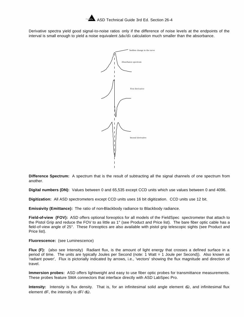
ASD Technical Guide 3rd Ed. Section 26-4
Derivative spectra yield good signal-to-noise ratios only if the difference of noise levels at the endpoints of the interval is small enough to yield a noise equivalent ∆dα/dλ calculation much smaller than the absorbance.
Difference Spectrum: A spectrum that is the result of subtracting all the signal channels of one spectrum from another. Digital numbers (DN): Values between 0 and 65,535 except CCD units which use values between 0 and 4096. Digitization: All ASD spectrometers except CCD units uses 16 bit digitization. CCD units use 12 bit. Emissivity (Emittance): The ratio of non-Blackbody radiance to Blackbody radiance. Field-of-view (FOV): ASD offers optional foreoptics for all models of the FieldSpec spectrometer that attach to the Pistol Grip and reduce the FOV to as little as 1° (see Product and Price list). The bare fiber optic cable has a field-of-view angle of 25°. These Foreoptics are also available with pistol grip telescopic sights (see Product and Price list). Fluorescence: (see Luminescence) Flux (F): (also see Intensity) Radiant flux, is the amount of light energy that crosses a defined surface in a period of time. The units are typically Joules per Second (note: 1 Watt = 1 Joule per Second)). Also known as 'radiant power', Flux is pictorially indicated by arrows, i.e., 'vectors' showing the flux magnitude and direction of travel. Immersion probes: ASD offers lightweight and easy to use fiber optic probes for transmittance measurements. These probes feature SMA connectors that interface directly with ASD LabSpec Pro. Intensity: Intensity is flux density. That is, for an infinitesimal solid angle element dΩ, and infinitesimal flux element dF, the intensity is dF/ dΩ.
Absorbance spectrum
First derivative
Second derivative
Sudden change in the curve
ASD Technical Guide 3rd Ed. Section 26-5
Isotropic Medium: Material in which light energy may impinge upon or travel through without any energy changes due to position or direction. Log(1/Reflectance): A commonly used math pretreatment, useful for linearizing reflectance data. This expression is often abbreviated as log(1/R). In most cases it is possible to find a linear correlation of log(1/R) data to concentration of an analyte in the target matrix. However, a general derivation relating reflectance to concentration cannot be rigorously derived, such as, the Bouguer-Lambert-Beer law for transmittance. Luminescence: Sometimes, a photon incident on a sample is absorbed, causing an electron to jump from its ground state to a higher, excited, energy state. Around 10
-8 seconds later, the electron returns to the ground state
resulting in an emission of a photon of a different wavelength than the incident photon. This return to the ground state also results in an excited vibrational state which reaches equilibrium in about 10
-12 seconds. Altogether, these events are called luminescence. There are two types of luminescence that are
distinguished by their ground and excited states: fluorescence and phosphorescence. The incident photons associated with luminescence are called the "excitation source". Luminescence and inelastic scattering are different and separate events even though it is difficult to differentiate the resulting photons. Except for highly viscous liquids, fluorescence of solutions is always unpolarized even if the excitation source is highly polarized. The wavelength of the fluorescing photons is always longer than the excitation source. The ratio of the energies of fluorescing photons to excitation source is typically less than 0.01. Maintenance: All ASD manufactured products come with a full 1 year limited warranty. Optional service contracts that take effect at warranty expiration are also available at additional cost (see Product & Price lists). Monochromator: Optical device for isolating a very narrow wavelength region of a radiant energy source. The isolation element may be any or combinations of the following: filters, gratings, prisms, and slits. Noise -equivalent-Delta-Radiance (Ne ∆∆ L or NeDL or NER): Defined as the radiance at a signal-to-noise ratio of unity. These values have been determined by viewing a stable, NIST traceable, radiance source with the FieldSpec spectroradiometer, and from the radiometric accuracy of the calibration source quoted by its manufacturer, Optronics Laboratory. NOTE: Standard built-in spectrum averaging function allows up to 31,800 spectra to be averaged thereby reducing the associated NeDL by a factor of the square root of the number of scans averaged. (also see Signal-to-noise ratio). Offset: Systematic noise including 'Dark-Current'. Photon: There are two models for radiant energy, the particle model and the wave model. In the particle model, radiant energy is comprised of discrete packets called photons. A photon's electromagnetic energy is defined as: Ephoton = hf, where h is Planck's constant and f is the frequency of the electromagnetic energy The energy amplitude measured at a specific wavelength of frequency f is determined by the number of photons at that wavelength, i.e., amplitude for the wave model is equivalent to numbers of photons for the particle model. Photodiode Array (PDA): (also see Charge Coupled Device) A PDA is a line of contiguous detectors manufactued into a single chip. Post-dispersive Spectrophotometers: All ASD spectrometers are “post-dispersive”. Because portable spectrometers are typically used outside the controlled laboratory environment, they are exposed to much higher levels of ambient light. In almost all cases, some of this ambient light will stray into the sample being measured. The errors produced by this ambient stray light are much greater for a pre-dispersive spectrometer than they are for a spectrometer that is post-dispersive. In a pre-dispersive spectrometer, the sample is illuminated with monochromatic light. Light scattered off or transmitted through the sample is then collected and delivered to the instrument’s detector. Ambient light that strays into the sample being measured is also collected. Thus, both the monochromatic illumination from the instrument and all wavelengths of the ambient stray light are delivered to the detector. Because the stray ambient light signal can represent a large fraction of the total light signal measured by the detector, it is a major source of error. While this source or error can be minimized by completely shielding the sample form all sources of ambient
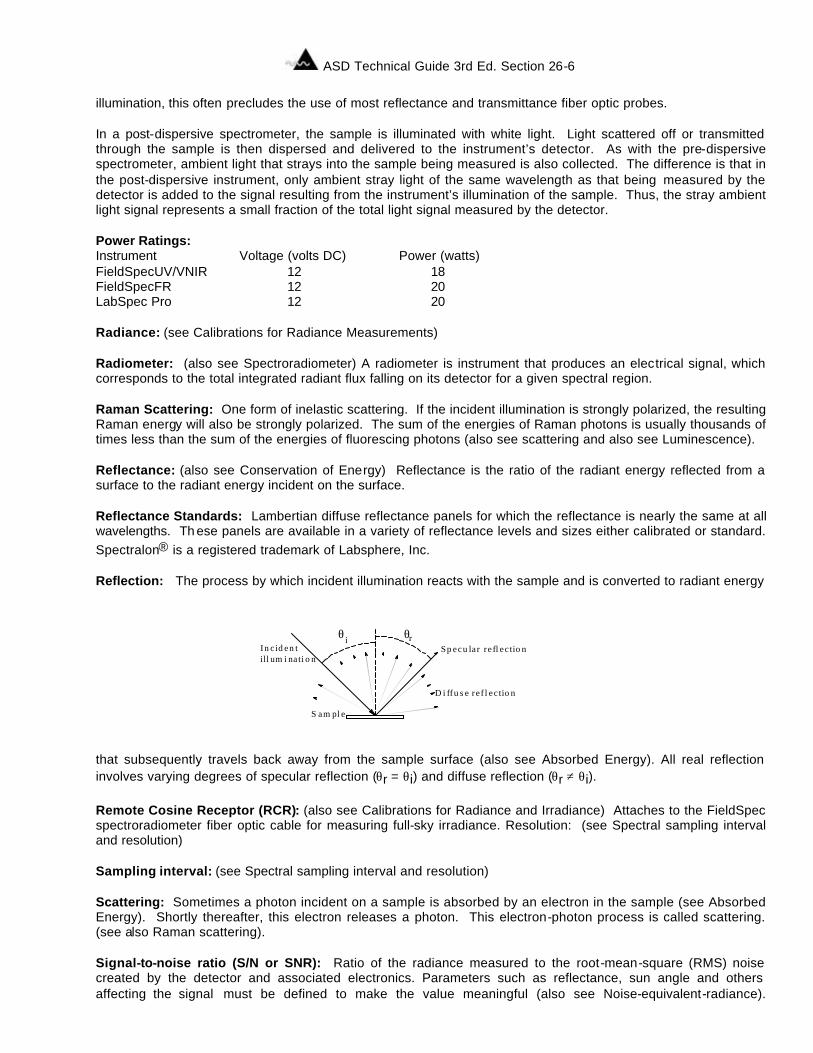
ASD Technical Guide 3rd Ed. Section 26-6
illumination, this often precludes the use of most reflectance and transmittance fiber optic probes. In a post-dispersive spectrometer, the sample is illuminated with white light. Light scattered off or transmitted through the sample is then dispersed and delivered to the instrument’s detector. As with the pre-dispersive spectrometer, ambient light that strays into the sample being measured is also collected. The difference is that in the post-dispersive instrument, only ambient stray light of the same wavelength as that being measured by the detector is added to the signal resulting from the instrument’s illumination of the sample. Thus, the stray ambient light signal represents a small fraction of the total light signal measured by the detector. Power Ratings: Instrument Voltage (volts DC) Power (watts) FieldSpecUV/VNIR 12 18 FieldSpecFR 12 20 LabSpec Pro 12 20 Radiance: (see Calibrations for Radiance Measurements) Radiometer: (also see Spectroradiometer) A radiometer is instrument that produces an electrical signal, which corresponds to the total integrated radiant flux falling on its detector for a given spectral region. Raman Scattering: One form of inelastic scattering. If the incident illumination is strongly polarized, the resulting Raman energy will also be strongly polarized. The sum of the energies of Raman photons is usually thousands of times less than the sum of the energies of fluorescing photons (also see scattering and also see Luminescence). Reflectance: (also see Conservation of Energy) Reflectance is the ratio of the radiant energy reflected from a surface to the radiant energy incident on the surface. Reflectance Standards: Lambertian diffuse reflectance panels for which the reflectance is nearly the same at all wavelengths. Th ese panels are available in a variety of reflectance levels and sizes either calibrated or standard. Spectralon® is a registered trademark of Labsphere, Inc. Reflection: The process by which incident illumination reacts with the sample and is converted to radiant energy
that subsequently travels back away from the sample surface (also see Absorbed Energy). All real reflection involves varying degrees of specular reflection (θr = θi) and diffuse reflection (θr ≠ θi). Remote Cosine Receptor (RCR): (also see Calibrations for Radiance and Irradiance) Attaches to the FieldSpec spectroradiometer fiber optic cable for measuring full-sky irradiance. Resolution: (see Spectral sampling interval and resolution) Sampling interval: (see Spectral sampling interval and resolution) Scattering: Sometimes a photon incident on a sample is absorbed by an electron in the sample (see Absorbed Energy). Shortly thereafter, this electron releases a photon. This electron-photon process is called scattering. (see also Raman scattering). Signal-to-noise ratio (S/N or SNR): Ratio of the radiance measured to the root-mean-square (RMS) noise created by the detector and associated electronics. Parameters such as reflectance, sun angle and others affecting the signal must be defined to make the value meaningful (also see Noise-equivalent-radiance).
Sp ecu lar re fl ec tio nrθ
In c id en till um i na ti o n
S am pl e
iθ
D i ffu s e re f l ec tio n
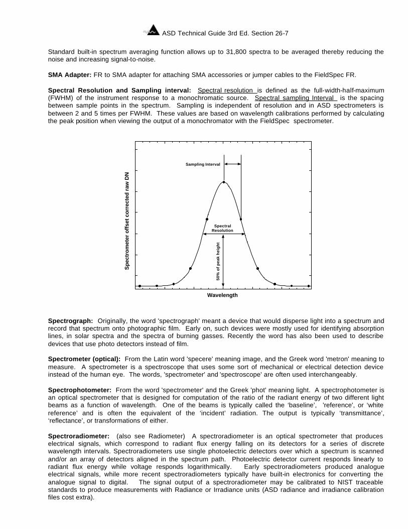
ASD Technical Guide 3rd Ed. Section 26-7
Standard built-in spectrum averaging function allows up to 31,800 spectra to be averaged thereby reducing the noise and increasing signal-to-noise. SMA Adapter: FR to SMA adapter for attaching SMA accessories or jumper cables to the FieldSpec FR. Spectral Resolution and Sampling interval: Spectral resolution is defined as the full-width-half-maximum (FWHM) of the instrument response to a monochromatic source. Spectral sampling Interval is the spacing between sample points in the spectrum. Sampling is independent of resolution and in ASD spectrometers is between 2 and 5 times per FWHM. These values are based on wavelength calibrations performed by calculating the peak position when viewing the output of a monochromator with the FieldSpec spectrometer. Spectrograph: Originally, the word 'spectrograph' meant a device that would disperse light into a spectrum and record that spectrum onto photographic film. Early on, such devices were mostly used for identifying absorption lines, in solar spectra and the spectra of burning gasses. Recently the word has also been used to describe devices that use photo detectors instead of film. Spectrometer (optical): From the Latin word 'specere' meaning image, and the Greek word 'metron' meaning to measure. A spectrometer is a spectroscope that uses some sort of mechanical or electrical detection device instead of the human eye. The words, 'spectrometer' and 'spectroscope' are often used interchangeably. Spectrophotometer: From the word 'spectrometer' and the Greek 'phot' meaning light. A spectrophotometer is an optical spectrometer that is designed for computation of the ratio of the radiant energy of two different light beams as a function of wavelength. One of the beams is typically called the ‘baseline’, 'reference', or ‘white reference’ and is often the equivalent of the ‘incident’ radiation. The output is typically ‘transmittance’, ‘reflectance’, or transformations of either. Spectroradiometer: (also see Radiometer) A spectroradiometer is an optical spectrometer that produces electrical signals, which correspond to radiant flux energy falling on its detectors for a series of discrete wavelength intervals. Spectroradiometers use single photoelectric detectors over which a spectrum is scanned and/or an array of detectors aligned in the spectrum path. Photoelectric detector current responds linearly to radiant flux energy while voltage responds logarithmically. Early spectroradiometers produced analogue electrical signals, while more recent spectroradiometers typically have built-in electronics for converting the analogue signal to digital. The signal output of a spectroradiometer may be calibrated to NIST traceable standards to produce measurements with Radiance or Irradiance units (ASD radiance and irradiance calibration files cost extra).
Wavelength
Sampling Interval
SpectralResolution
50%
of
pea
k h
eig
ht
Spe
ctro
met
er o
ffse
t cor
rect
ed r
aw D
N
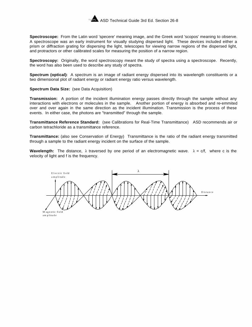
ASD Technical Guide 3rd Ed. Section 26-8
Spectroscope: From the Latin word 'specere' meaning image, and the Greek word 'scopos' meaning to observe. A spectroscope was an early instrument for visually studying dispersed light. These devices included either a prism or diffraction grating for dispersing the light, telescopes for viewing narrow regions of the dispersed light, and protractors or other calibrated scales for measuring the position of a narrow region. Spectroscopy: Originally, the word spectroscopy meant the study of spectra using a spectroscope. Recently, the word has also been used to describe any study of spectra. Spectrum (optical): A spectrum is an image of radiant energy dispersed into its wavelength constituents or a two dimensional plot of radiant energy or radiant energy ratio versus wavelength. Spectrum Data Size: (see Data Acquisition) Transmission: A portion of the incident illumination energy passes directly through the sample without any interactions with electrons or molecules in the sample. Another portion of energy is absorbed and re-emmited over and over again in the same direction as the incident illumination. Transmission is the process of these events. In either case, the photons are "transmitted" through the sample. Transmittance Reference Standard: (see Calibrations for Real-Time Transmittance) ASD recommends air or carbon tetrachloride as a transmittance reference. Transmittance: (also see Conservation of Energy) Transmittance is the ratio of the radiant energy transmitted through a sample to the radiant energy incident on the surface of the sample. Wavelength: The distance, λ traversed by one period of an electromagnetic wave. λ = c/f, where c is the velocity of light and f is the frequency.
λ
D is ta n c e
E l e c tr ic fi e ld
a m p li tud e
M a g n e tic fi e lda m p li tu d e
ASD Technical Guide 3rd Ed. Section 27-1
Section 27 Reprints
Insert Reprints: Ground Truthing Spectrometers Nitrogen Deficiency Detection CERES Experiment Provides Camo: Patterns Issues in Absolute Spectral Radiometric Photonics Diffuser Clarifies A Comparison of Near-Infrared Spectrometers for Insert Reprint:

ASD Technical Guide 3rd Ed. Section 27-2

ASD Technical Guide 3rd Ed. Section 28-1
Section 28 Price List
Insert Price List Here

ASD Technical Guide 3rd Ed. Section 28-2