Embed Size (px)
Citation preview

1
/0975/
Front. Environ. Sci. Engin. China 2009, 3(1): 112-128 DOl 10.1007/s11783-008-0067-z
Analytical solutions of three-dimensional contaminant transport in uniform flow field in porous media: A library
Hongtao WANG ([8J), Huayong WU
Department of Environmental Science and Engineering, Tsinghua University, Beijing 100084, China
© Higher Education Press and Springer-Verlag 2008
Abstract The purpose of this study is to present a library of analytical solutions for the three-dimensional contaminant transport in uniform flow field in porous media with the first-order decay, linear sorption, and zero-order production. The library is constructed using Green's function method (GFM) in combination with available solutions. The library covers a wide range of solutions for various conditions. The aquifer can be vertically finite, semi-infinitive or infinitive, and laterally semi-infinitive or infinitive. The geometry of the sources can be of point, line, plane or volumetric body; and the source release can be continuous, instantaneous, or by following a given function over time. Dimensionless forms of the solutions are also proposed. A computer code FlowCAS is developed to calculate the solutions. Calculated results demonstrate the correctness of the presented solutions. The library is widely applicable to solve contaminant transport problems of one- or multiple- dimensions in uniform flow fields.
Keywords solution library, contaminant transport, analytical solution, dispersion and advection, porous media, type curve, Green's function method (GFM)
Introduction
Analytical solutions of contaminant transport in porous media can be applied in many fields. They can provide better physical insights into the problems; thus, are the basic tools to reveal the mechanism of contaminant transport phenomena. Analytical solutions can help us to analyze the influence of parameters and boundary conditions, measure the field parameters related to contaminant transport, and verify the numerical models, as they are free of numerical dispersions attached to numerical simulations, especially in the advection dominated transport [J]. They can also be used to predict the movement of
Received February 26, 2008; accepted May 8, 2008
E-mail: [email protected]
33853
11"1" III" 111'1 1'1'1 'II" IIII 1"1
contaminant plumes and design the experiments III the field or laboratory scales [2].
Analytical solutions of contaminant transport have been widely studied in the last three decades. Many solutions have been published before and new ones are still appearing. For instance, Cleary and Adrian [3], Sauty and Pierre [4], and van Genuchten [5] have provided analytical solutions for one-dimensional transport with the first-type (Dirichlet) and third-type (Cauchy) boundary conditions, respectively. Hunt [6], Latinopoulos et al [7], and Wilson and Miller [8] have investigated the two dimensional transport models for the continuous release of a point source. Batu has studied the two-dimensional analytical solutions for the plane sources with the first- and the second-type boundary conditions [9,10]. Quezada and Clement developed a generalized solution to multi-dimensional multi-species transport equations coupled through sequential first-order reactions [11]. Recently, Srinivasan and Clement derived a closed-form solution to the problem [12,13].
For the study of three-dimensional contaminant transport in uniform flow field, one of the most widely used analytical solutions is the approximate one proposed by Domenico [14,15]. The solution is expressed in a simple way without integration. Neville has obtained the solution for the vertical rectangle source by taking the source as the boundary condition of the first type [16]. Leij et al. have studied the analytical solutions for non-equilibrium solute transport in three-dimensional porous media using the Laplace, Fourier, and Hankel transforms [17,18]. Later in 2000, Leij et al. have provided a useful Green's function table using the Green's function method (GFM) for various plane sources that can be used to construct solutions [19]. They also illustrated three solutions for a semiinfinitive aquifer. Park and Zhan obtained a series of analytical solutions of contaminant transport from finite one-, two-, and three- dimensional sources in a finitethickness aquifer by GFM [20]. In addition, many other authors have also published some solutions for different sources and boundary conditions [21-26].

The purpose of this paper is to present a library ofanalytical solutions of contaminant transport in uniformflow field in porous media. The users can either use thesolutions presented in the paper or construct their ownsolutions by using the directional solutions and theirintegration results over directional source lengths to solvetheir specific problems. The types of contaminant sourcescan be of point, line, plane or volumetric body; theirrelease duration can be instantaneous, temporary or con-tinuous and their strengths or concentrations can be con-stant or variable over time. The first-order decay orattenuation and linear retardation process (Henry mod-ule) are considered. The aquifer can be vertically infin-itive, semi-infinitive or finite and horizontally infinitiveor semi-infinitive. By using the method of imaging andsuperposition principles, the problems of linear bound-aries, multiple sources, sources of irregular shapes, andrandom change of source strengths and concentrationscan also be solved.
2 Mathematical model and solutionmethods
2.1 Assumptions
The assumptions embedded in the analytical solutions areactually the constraint conditions for their application.Therefore, it is important to know the conditions andlimitations before we make use of the solutions for prac-tical purpose. The following conditions are assumed inthis study:Studied domain The aquifer or the studied domain is
vertically finite with constant thickness or semi-finite,horizontally infinite or semi-finite in x- or y-directions,homogeneous, and anisotropic.Source type There exist sources of point, line, plane or
volumetric body, either regular or irregular in shape. Theycan be treated either as a source term inside the domain oras a boundary condition if the source concentration isprovided. The corresponding domain for the former caseis horizontally infinite, while for the latter case, is hori-zontally semi-finite. The source strength can be constantor time-dependent but not space- independent.Flow field Fluid flow is steady and uniform along the x-
or xz-directions.Retardation Partitioning between dissolved and sorbed
phases is instantaneous and reversible, and can be repre-sented by the linear sorption process.Attenuation Solute undergoes first-order degradation
or decay. The rate constants can be the same or differentin the dissolved and sorbed phases, or zero in the sorbedphase.Initial condition There is no target contaminant in the
studied domain at the initial time.
Transport The contaminant transport in the domain isassumed to be three-dimensional. The components ofhydrodynamic dispersion coefficient tensor are knownwith its principal directions parallel to the x-, y-, and z-axis respectively.It should be noted that from the view of the constraints
applied for the analytical solutions, the above assump-tions are relatively widely applicable, compared to morestrict constraints embedded in other known analyticalsolutions.
2.2 Mathematical model
The three-dimensional advection- dispersion equationwith first-order decay and zero order source or productionunder the above assumptions can be written as [2]
LðCÞ ¼ I=n, (1)
where the linear operator L is defined by
LðCÞ ¼ ∂C∂t
–Dx∂2C∂x2
–Dy∂2C∂y2
–Dz∂2C∂z2
þu∂C∂x
þ lC, (2)
and subject to initial condition
Cðx,y,z,tÞjt¼0 ¼ 0,x,y,z∈D, (3)
and boundary conditions of various types, which will bediscussed later, where C(x, y, z, t) [ML–3] is the soluteconcentration at location (x, y, z) at time t; Dx, Dy, andDz [L
2T–1] are principal dispersion coefficients; l [T–1] isthe first-order constant for decay in liquid and sorbedphases; u [LT–1] is the pore- water velocity along the x-axis; b [L] and n are the thickness and the porosity of theaquifer, respectively; D is the studied domain; and I[ML–3T–1] is the zero-order source term.Note that I exists only in the space occupied by the
source, while for the rest of the domain, I is equal to zero.For instance, if source occupies a space of parallelepipedbody, x 2 [0, x0], y 2 [ – y0, y0], and z 2 [z0, z1],
I ¼ I0f ðtÞ, 0 < x < x0, – y0 < y < y0, z0 < z < z1, t > 0,
0, otherwise,
((4)
where I0 [ML–3T–1] is the initial volumetric mass released bythe source per unit time; f(t) is a dimensionless knownfunction, representing the changes of source strength withtime.The boundary conditions are set as follows:1) Horizontal infinitive boundaries If the source term
is inside the domain and source strength is provided,the horizontal domain is set to infinitive and the con-centration in infinitive boundaries is set to zero, that is,
Hongtao WANG et al. Solutions library of three-dimensional contaminant transport in uniform flow field in porous media 113

Cðx,y,z,tÞjx!�1 ¼ 0, t > 0; (5)
Cðx,y,z,tÞjy!�1 ¼ 0, t > 0: (6)
2) Horizontal semi-infinitive boundaries If the sourceconcentration is provided, it can be treated as a boundarycondition of the first type. The function of sources is imple-mented by the boundary condition while I in Equation (1)is set to zero. For instance, if a vertical rectangle source isalong the yz- plane at x = 0, the studied domain can be setto semi- infinitive in the x-direction, x 2 [0, +1), and theboundary condition at x = 0 is expressed as
Cðx,y,z,tÞjx¼0 ¼C0, y, z∈source, t > 0,
0, otherwise:
((7)
3) Vertical infinitive boundaries If an aquifer can beconsidered as infinitive in thickness, the vertical domainin the z-direction is infinitive, and the vertical infinitiveboundary is set to the first type as
Cðx,y,z,tÞjz!�1 ¼ 0, t > 0: (8)
4) Vertical semi-infinitive boundaries with the sourceconcentration provided on top boundaries The verticaldomain is z 2 [0, +1), and the top boundary condition is
Cðx,y,z,tÞjz¼0 ¼C0, x, y∈source , t > 0,
0, otherwise:
((9)
5) Vertical finite boundaries If an aquifer is of constantthickness, b, the vertical domain is z 2 [0, b]. It is assumedthat the contaminant can not penetrate through the topand bottom boundaries, that is,
∂C∂z
����z¼0
¼ ∂C∂z
����z¼b
¼ 0, –1 < x,y < 1, t > 0: (10)
2.3 Solution method
Solutions to Eq. (1) exist for a variety of boundary con-ditions as stated above. The solutions can be derived bymaking use of traditional integration transform methods,such as Laplace method, or more recent Green’s functionmethod (GFM). The GFM can be briefly described in thefollowing steps [19,20,27,28]:1) Deriving the solutions for an instantaneous point
source in an infinitive, semi-finite and finite aquifer. Thegoverning equation for an infinite aquifer is
LðCÞ ¼ Mp
nδðx – x0 ,y – y0
,z – z0,t – τÞ, (11)
and the corresponding differential equation of the Green’sfunction is [19,29]
L�ðGÞ ¼ δðx – x0,y – y
0,z – z
0,t – τÞ, (12)
where L* is the adjoint differential operator:
L�ðGÞ ¼ –∂G∂τ
–Dx∂2G∂x02
– u∂G∂x0 –Dy
∂2G∂y02
–Dz∂2G∂z02
þ lG,
(13)
where G is the Green’s function; Mp [M] is the massreleased instantaneously at point (x′, y′, z′) at time τ; δ[L–3T–1] is the Dirac delta function.The GFM indicates that a three-dimensional solution
is the product of the three directional solutions [19,27].The directional solutions for directions x, y and z withdifferent boundary conditions are summarized inTable 1. For instance, the directional solution in thex-direction for an instantaneous point source is shownin Eq. (14).Note that if an aquifer is vertically semi-finite or finite
with a constant thickness b, the contaminant cannot pen-etrate through its top or bottom boundaries. To solve theproblem, the method of imaging is applied [30]. Take thefinite thick aquifer as an example, the source and the topand bottom boundaries are imaged for infinite numbers oftimes in the z-direction. Therefore, the boundary valueproblem can be represented by a vertically infinitive prob-lem with infinite numbers of the image sources and theoriginal source [20,2], as shown in Eq. (20).From Table 1 it is easy to construct solutions for the
instantaneous point sources. For instance, the analyticalsolutions for the infinitively and finitely thick aquifers are[20,29]
Cðx,y,z,tÞ ¼ Mp
8nffiffiffiffiffiffiffiffiffiffiffiffiffiffiffiffiffiffiffiffiffiffiffiffiffiffiffiffiffiffiffiffiffip3DxDyDzðt – τÞ3
q exp½ – lðt – τÞ�
�exp –½ðx – x0 Þ – uðt – τÞ�2
4Dxðt – τÞ
)(
�exp –ðy – y0 Þ24Dyðt – τÞ
" #exp –
ðz – z0 Þ24Dzðt – τÞ
" #, (22)
and
Cðx,y,z,tÞ ¼ Mp
4pnbðt – τÞ ffiffiffiffiffiffiffiffiffiffiffiDxDy
p exp½ – lðt – τÞ�
�exp –½ðx – x0 Þ – uðt – τÞ�2
4Dxðt – τÞ
)(
�exp –ðy – y0 Þ24Dyðt – τÞ
" #1þ 2
X1n¼1
cosnpðz0 – z
0 Þb
"
�cosnpðz – z0 Þ
bexp –
Dzn2p2
b2ðt – τÞ
� �#, (23)
114 Front. Environ. Sci. Engin. China 2009, 3(1): 112–128

respectively. When τ = 0, Eqs. (22) and (23) becomes thesolutions for the point source of initially instantaneousrelease [20,2].2) Obtaining the instantaneous solutions by an analytic
integration over the length, area or volume of the source.Taking the above mentioned parallelepiped body sourceas an example, the source body is located at x 2 [0, x0],y 2 [ – y0, y0], and z 2 [z0, z1]. For an infinitively wide andinfinitively thick aquifer,
Cðx,y,z,tÞ ¼ Mv
8nffiffiffiffiffiffiffiffiffiffiffiffiffiffiffiffiffiffiffiffiffiffiffiffiffiffiffiffiffiffiffiffiffip3DxDyDzðt – τÞ3
q exp½ – lðt – τÞ�
�!x0
0!
y0
– y0!
z1
z0exp –
½ðx – x0 Þ – uðt – τÞ�24Dxðt – τÞ
)(
�exp –ðy – y0 Þ24Dyðt – τÞ
" #exp –
ðz – z0 Þ24Dzðt – τÞ
" #dx
0dy
0dz
0:
(24)
The results of the analytic integration over the sourcelength in the corresponding direction, which can be usedto construct analytical solutions for various conditions,are summarized in Table 2 for the infinitive, semi-infin-itive, and finite boundaries.
From Eq. (24) referred to Table 2, we can easily obtainthe analytical solution of the instantaneous release from avolumetric source:
Cðx,y,z,tÞ ¼ Mv
8nexp½ – lðt – τÞ� erfc
x – uðt – τÞ – x02ffiffiffiffiffiffiffiffiffiffiffiffiffiffiffiffiffiDxðt – τÞ
p"
– erfcx – uðt – τÞ2ffiffiffiffiffiffiffiffiffiffiffiffiffiffiffiffiffiDxðt – τÞ
p#
� erfcy – y0
2ffiffiffiffiffiffiffiffiffiffiffiffiffiffiffiffiffiDyðt – τÞ
p – erfcyþ y0
2ffiffiffiffiffiffiffiffiffiffiffiffiffiffiffiffiffiDyðt – τÞ
p" #
� erfcz – z0
2ffiffiffiffiffiffiffiffiffiffiffiffiffiffiffiffiffiDzðt – τÞ
p – erfczþ z0
2ffiffiffiffiffiffiffiffiffiffiffiffiffiffiffiffiffiDzðt – τÞ
p" #
, (30)
where Mv [ML–3] is the mass released instantaneouslyat time τ per unit source volume. Similarly, we canobtain the solutions for a finitely thick aquifer. If τ = 0,Eq. (30) becomes the solution for initially instantaneousrelease.3) Obtaining the solutions of continuous source release
by analytic integration of instantaneous release solutionsover time. For a continuous source, integration of Eq. (30)
Table 1 Directional solutions for the instantaneous point sources
direction condition directional solution
x Cjx!�1 ¼ 0
–1 < x < þ1 Gx ¼1
2ffiffiffiffiffiffiffiffiffiffiffiffiffiffiffiffiffiffiffipDxðt – τÞ
p exp –½ðx – x0 Þ – uðt – τÞ�2
4Dxðt – τÞ
)((14)
Cjx¼0 ¼(C0,ðy,zÞ∈source
0,otherwise0 < x < þ1
Gx ¼x – x
0
2ffiffiffiffiffiffiffiffiffiffiffiffiffiffiffiffiffiffiffipDxðt – τÞ
p exp –½x – x0 – uðt – τÞ�2
4Dxðt – τÞ
( )(15)
y Cjy!�1 ¼ 0
–1 < y < þ1 Gy ¼1
2ffiffiffiffiffiffiffiffiffiffiffiffiffiffiffiffiffiffiffipDyðt – τÞ
p exp –ðy – y0 Þ24Dyðt – τÞ
" #(16)
Cjy¼0 ¼(C0,ðx,zÞ∈source
0,otherwise0 < y < þ1
Gy ¼y – y
0
2ffiffiffiffiffiffiffiffiffiffiffiffiffiffiffiffiffiffiffipDyðt – τÞ
p exp –ðy – y0 Þ24Dyðt – τÞ
" #(17)
z Cjz!�1 ¼ 0
–1 < z < þ1 Gz ¼1
2ffiffiffiffiffiffiffiffiffiffiffiffiffiffiffiffiffiffiffipDzðt – τÞ
p exp –ðz – z0 Þ24Dzðt – τÞ
" #(18)
∂C=∂zjz¼0 ¼ 0
Cjz!þ1 ¼ 0
0£z < þ1
Gz ¼1
2ffiffiffiffiffiffiffiffiffiffiffiffiffiffiffiffiffiffiffipDzðt – τÞ
p exp –ðz – z0 Þ24Dzðt – τÞ
" #þ exp –
ðzþ z0 Þ2
4Dzðt – τÞ
" #( )(19)
∂C=∂zjz¼0 ¼ 0
∂C=∂zjz¼b ¼ 0
0£z£b
Gz ¼1
b1þ 2
X1m¼1
cosmpðz0 – z
0 Þb
cosmpðz – z0 Þ
bexp –
Dzn2p2
b2ðt – τÞ
� �( )(20)
Cjz¼0 ¼(C0,ðx,yÞ∈source
0,otherwise0 < z < þ1
Gz ¼z – z
0
2ffiffiffiffiffiffiffiffiffiffiffiffiffiffiffiffiffiffiffipDzðt – τÞ
p exp –ðx – x0 Þ24Dzðt – τÞ
" #(21)
Hongtao WANG et al. Solutions library of three-dimensional contaminant transport in uniform flow field in porous media 115

over time from 0 to t yields
Cðx,y,z,tÞ ¼ I08n!
t
0f ðt – τÞexpð – lτÞ
� erfcx – uτ – x02ffiffiffiffiffiffiffiffiDxτ
p – erfcx – uτ
2ffiffiffiffiffiffiffiffiDxτ
p� �
� erfcy – y02ffiffiffiffiffiffiffiffiDyτ
p – erfcyþ y02ffiffiffiffiffiffiffiffiDyτ
p" #
� erfcz – z12ffiffiffiffiffiffiffiDzτ
p – erfcz – z02ffiffiffiffiffiffiffiDzτ
p� �
dτ: (31)
3 Solution library
By using the above stated GFM in combinations withsuperposition principle and imaging method, a library ofanalytical solutions is constructed for a three-dimensionalcontaminant transport in a uniform flow field.
3.1 Solutions for continuous release
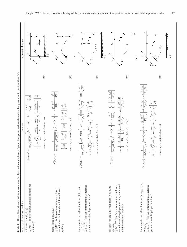
Solutions for the regular continuous source release aresummarized in Table 3, with the source types of point,line, plane, and parallel-piped body in a finite and semi-finite aquifer. Some solutions in the Table have been pub-lished by other authors as noted, and some are, for thefirst time, constructed by using the equations in Tables 1and 2. For the practical application of the solutions, usersmust be aware of the conditions and constraints embed-ded with them.
Equations in Table 3 can be easily simplified to obtainthe solutions for one- or two-dimensional transportproblems. For instance, by letting z0 equal to 0 and z1 tob in Eq. (38), the solution of two-dimensional transport isobtained for a point source in horizontal plane view,which is identical to the solution proposed by Wilsonand Miller [8].Most analytical solutions shown in Table 3 include
the temporal integrations. In general, the integrationsare often evaluated numerically. In this paper, theGaussian Quadrature method is utilized to numericallyevaluate integrations. A computer code named Flow-CAS (Flow and Contaminant transport AnalyticalSolutions) is created by using Borland Delphi 7. Thecode can make calculations of all solutions presented inthis paper.
3.2 Solutions for instantaneous release
As mentioned in the above section, solutions for theinstantaneous release are the basis for deriving the solu-tions for continuous release. Therefore, the solutions inTable 3 can be easily modified to yield the solutions forinstantaneous release. For the cases of given sourcestrengths, by substituting Mp, Ml, Ma, and Mv for Ip, Il,Ia, and I, respectively, taking out of the temporal integ-ration, and substituting t for τ, the corresponding equa-tions in the Table then become the solutions for theinstantaneous release, where Ml [ML–1] and Ma [ML–2]are the mass released per unit source length and per unitsource area, respectively. For instance, the solution for theinstantaneous release of a point source in a finite aquiferis, according to Eq. (32):
Table 2 Results of the integration of directional solutions over the source lengths
sourcerange
condition integration result
0 – x0 Cjx!�1 ¼ 0
–1 < x < þ11
2erfc
x – uðt – τÞ – x02ffiffiffiffiffiffiffiffiffiffiffiffiffiffiffiffiffiDxðt – τÞ
p – erfcx – uðt – τÞ2ffiffiffiffiffiffiffiffiffiffiffiffiffiffiffiffiffiDxðt – τÞ
p" #
(25)
– y0 – y0 Cjy!�1 ¼ 0
–1 < y < þ11
2erfc
y – y02ffiffiffiffiffiffiffiffiffiffiffiffiffiffiffiffiffiDyðt – τÞ
p – erfcyþ y0
2ffiffiffiffiffiffiffiffiffiffiffiffiffiffiffiffiffiDyðt – τÞ
p" #
(26)
z0 – z1 Cjz!�1 ¼ 0
–1 < z < þ11
2erfc
z – z12ffiffiffiffiffiffiffiffiffiffiffiffiffiffiffiffiffiDzðt – τÞ
p – erfcz – z0
2ffiffiffiffiffiffiffiffiffiffiffiffiffiffiffiffiffiDzðt – τÞ
p" #
(27)
z0 – z1 ∂C=∂zjz¼0 ¼ 0
Cjz!þ1 ¼ 0
0£z < þ1
1
2erfc
z – z12ffiffiffiffiffiffiffiDzτ
p – erfcz – z02ffiffiffiffiffiffiffiDzτ
p þ erfczþ z02ffiffiffiffiffiffiffiDzτ
p – erfczþ z12ffiffiffiffiffiffiffiDzτ
p� �
(28)
z0 – z1 ∂C=∂zjz¼0 ¼ 0
∂C=∂zjz¼b ¼ 0
0£z£b
1
bz1 – z0 þ
2b
p
X1n¼1
1
nsin
npz1b
– sinnpz0b
� �cos
npzb
exp –Dzn
2p2
b2ðt – τÞ
� �" #(29)
116 Front. Environ. Sci. Engin. China 2009, 3(1): 112–128
Tab
le3
Three
dimension
alanalytical
solutio
nsforthecontinuo
usreleaseof
point,lin
e,planeandparallelepipedbo
dysourcesin
uniform
flow
field
source
type/bound
arycond
ition
solutio
nschematic
diagram
pointsource
at(0,0,
z 0).
(Ip[M
T–1]isthecontam
inantmassreleased
per
unittim
e.)a
Cðx,
y,z,tÞ¼
1
4pnb
ffiffiffiffiffiffiffiffiffiffiffi
DxD
y
p!t 0
I pðt–
τÞexp
–lτ–ðx–uτÞ2
4Dxτ
–y2
4Dyτ
��
�1þ2X1 m
¼1cosmpz
0
bcosmpz b
exp
–D
zm2p2
b2τ
��
"# d
τ τ
–1
<x,y<
1,0£z£
b,t>
0(32)
pointsource
at(0,0,
z 0)
(Ip[M
T–1]isthecontam
inantmassreleased
perunittim
e,in
thesemi-infinitiv
ethickness
aquifer.)
Cðx,
y,z,tÞ¼
1
8nðpÞ3=
2ffiffiffiffiffiffiffiffi
ffiffiffiffiffiffiffiffiD
xDyD
z
p!t 0
I pðt–
τÞexp
–lτ–ðx–uτÞ2
4Dxτ
–y2
4Dyτ
��
�exp
–ðz–z 0Þ2
4Dzτ
�� þ
exp
–ðzþz 0Þ2
4Dzτ
��
d
τ
τ3=2
–1
<x,y<
1,0£z<
1,t>
0(33)
linesource
inthex-directionfrom
(0,0,
z 0)to
(x0,0,
z 0)
(Il[M
L–1T–1]isthecontam
inantmassreleased
perun
itsource
leng
thperun
ittim
e.)a
Cðx,
y,z,tÞ¼
1
4nbffiffiffiffiffiffiffiffi pD yp
!t 0I lðt–
τÞexp
–lτ–
y2
4Dyτ
�� er
fcx–uτ
–x 0
2ffiffiffiffiffiffiffiffi D xτp
–erfc
x–uτ
2ffiffiffiffiffiffiffiffi D xτp
��
�1þ2X1 m
¼1cosmpz
0
bcosmpz b
exp
–D
zm2p2
b2τ
��
"# d
τ ffiffi τp–1
<x,y<
1,0£z£
b,t>
0(34)
linesource
inthex-directionfrom
(0,0,
z 0)to
(x0,0,
z 0)
(Il[M
L–1T–1]isthecontam
inantmassreleased
perun
itsource
leng
thperun
ittim
e,in
thesemi-
infinitiv
ethicknessaquifer.)
Cðx,
y,z,tÞ¼
1
8npffiffiffiffiffiffiffiffi
ffiffiffiD
yDz
p!t 0
I lðt–
τÞexp
–lτ–
y2
4Dyτ
�� �
exp
–ðz–z 0Þ2
4Dzτ
��
þexp
–ðzþz 0Þ2
4Dzτ
��
erfcx–uτ
–x 0
2ffiffiffiffiffiffiffiffi D xτp
–erfc
x–uτ
2ffiffiffiffiffiffiffiffi D xτp
�� dτ τ
–1
<x,y<
1,0£z<
1,t>
0(35)
linesource
inthey-directionfrom
(0,–y 0,z 0)to
(0,y 0,z 0)
(Il[M
L–1T–1]isthecontam
inantmassreleased
perun
itsource
length
perun
ittim
e.)a
Cðx,
y,z,tÞ¼
1
4nbffiffiffiffiffiffiffiffi pD xp
!t 0I lðt–
τÞexp
–lτ–ðx–uτÞ2
4Dxτ
�� er
fcy–y 0
2ffiffiffiffiffiffiffiffi D yτp
–erfc
yþy 0
2ffiffiffiffiffiffiffiffi D yτp
"#
�1þ2X1 m
¼1cosmpz
0
bcosmpz b
exp
–D
zm2p2
b2τ
��
"# d
τ ffiffi τp–1
<x,y<
1,0£z£
b,t>
0(36)
Hongtao WANG et al. Solutions library of three-dimensional contaminant transport in uniform flow field in porous media 117

(Contin
ued)
source
type/bound
arycond
ition
solutio
nschematic
diagram
linesource
inthey-directionfrom
(0,–y 0,z 0)to
(0,y 0,z 0)
(Il[M
L–1T–1]isthecontam
inantmassreleased
perun
itsource
leng
thperun
ittim
e,in
thesemi-
infinitiv
ethicknessaquifer.)
Cðx,
y,z,tÞ¼
1
8npffiffiffiffiffiffiffiffi
ffiffiffiD
xDz
p!t 0
I lðt–
τÞexp
–lτ–ðx–uτÞ2
4Dxτ
��
�exp
–ðz–z 0Þ2
4Dzτ
�� þ
exp
–ðzþz 0Þ2
4Dzτ
��
er
fcy–y 0
2ffiffiffiffiffiffiffiffi D yτp
–erfc
yþy 0
2ffiffiffiffiffiffiffiffi D yτp
"# d
τ τ
–1
<x,y<
1,0£z<
1,t>
0(37)
linesource
inthez-directionfrom
(0,0,
z 0)to
(0,
0,z 1)
(Il[M
L–1T–1]isthecontam
inantmassreleased
perun
itsource
leng
thperun
ittim
e.)a
Cðx,
y,z,tÞ¼
1
4pnb
ffiffiffiffiffiffiffiffiffiffiffi
DxD
y
p!t 0
I lðt–
τÞexp
–lτ–ðx–uτÞ2
4Dxτ
–y2
4Dyτ
��
�z 1–z 0
þ2b p
X1 m¼1
1 msinmpz
1
b–sinmpz
0
b
�� co
smpz b
exp
–D
zm2p2
b2τ
��
"# d
τ τ
–1
<x,y<
1,0£z£
b,t>
0(38)
linesource
inthez-directionfrom
(0,0,
z 0)to
(0,
0,z 1)
(Il[M
L–1T–1]isthecontam
inantmassreleased
perun
itsource
leng
thperun
ittim
e,in
thesemi-
infinitiv
ethicknessaquifer.)
Cðx,
y,z,tÞ¼
1
8npffiffiffiffiffiffiffiffi
ffiffiffiD
xDy
p!t 0
I lðt–
τÞexp
–lτ–ðx–uτÞ2
4Dxτ
–y2
4Dyτ
��
�erfc
z–z 1
2ffiffiffiffiffiffiffi D zτp
–erfc
z–z 0
2ffiffiffiffiffiffiffi D zτp
þerfc
zþz 0
2ffiffiffiffiffiffiffi D zτp
–erfc
zþz 1
2ffiffiffiffiffiffiffi D zτp
�� dτ τ
–1
<x,y<
1,0£z<
1,t>
0(39)
vertical
rectanglesource
intheyz
planeat
x=0,
y2[–
y 0,y 0],z2[z0,z 1]
(Ia[M
L–2T–1]isthecontam
inantmassreleased
perunitsource
area
perunittim
e.)a
Cðx,
y,z,tÞ¼
1
4nbffiffiffiffiffiffiffiffi pD xp
!t 0I aðt–
τÞexp
–lτ–ðx–uτÞ2
4Dxτ
�� er
fcy–y 0
2ffiffiffiffiffiffiffiffi D yτp
–erfc
yþy 0
2ffiffiffiffiffiffiffiffi D yτp
"#
�z 1–z 0
þ2b p
X1 m¼1
1 msinmpz
1
b–sinmpz
0
b
�� co
smpz b
exp
–D
zm2p2
b2τ
��
"# d
τ ffiffi τp–1
<x,y<
1,0£z£
b,t>
0(40)
118 Front. Environ. Sci. Engin. China 2009, 3(1): 112–128

(Contin
ued)
source
type/bound
arycond
ition
solutio
nschematic
diagram
vertical
boundary
intheyz
planeat
x=
0(The
rectanglesource
isin
y2[–
y 0,y 0],z2[z0,z 1];
Cj x¼
0¼
C0,whenðy,
zÞ∈source
0,otherwise
(where
C0
[ML–3]isthesource
concentration.)b
Cðx,
y,z,tÞ¼
C0x
4bffiffiffiffiffiffiffiffi pD xp
!t 0exp
–lτ–ðx–uτÞ2
4Dxτ
�� er
fcy–y 0
2ffiffiffiffiffiffiffiffi D yτp
–erfc
yþy 0
2ffiffiffiffiffiffiffiffi D yτp
"#
�z 1–z 0
þ2b p
X1 m¼1
1 msinmpz
1
b–sinmpz
0
b
�� co
smpz b
exp
–D
zm2p2
b2τ
��
"# d
τ
τ3=2
x>
0,–1
<y<
1,0£z£
b,t>
0(41)
vertical
rectanglesource
inthexz
planeat
y=0,
x2[0,x 0],z2[z0,z 1]
(Ia[M
L–2T–1]isthecontam
inantmassreleased
perun
itsource
area
perun
ittim
e.)a
Cðx,
y,z,tÞ¼
1
4nbffiffiffiffiffiffiffiffi pD yp
!t 0I aðt–
τÞexp
–lτ–
y2
4Dyτ
�� er
fcx–uτ
–x 0
2ffiffiffiffiffiffiffiffi D xτp
–erfc
x–uτ
2ffiffiffiffiffiffiffiffi D xτp
��
�z 1–z 0
þ2b p
X1 m¼1
1 msinmpz
1
b–sinmpz
0
b
�� co
smpz b
exp
–D
zm2p2
b2τ
��
"# d
τ ffiffi τp–1
<x,y<
1,0£z£
b,t>
0(42)
horizontal
rectanglesource
inthexy
planeat
z=z 0,x2[0,x 0],y2[–
y 0,y 0]
(Ia[M
L–2T–1]isthecontam
inantmassreleased
persource
area
perunittim
e.)a
Cðx,
y,z,tÞ¼
1 4nb!t 0
I aðt–
τÞexpð–
lτÞ
erfcx–uτ
–x 0
2ffiffiffiffiffiffiffiffi D xτp
–erfc
x–uτ
2ffiffiffiffiffiffiffiffi D xτp
��
�erfc
y–y 0
2ffiffiffiffiffiffiffiffi D yτp
–erfc
yþy 0
2ffiffiffiffiffiffiffiffi D yτp
"# 1
þ2X1 m
¼1cosmpz
0
bcosmpz b
exp
–D
zm2p2
b2τ
��
"# d
τ
–1
<x,y<
1,0£z£
b,t>
0(43)
horizontal
boundary
inthexy
planeat
z=0
(The
rectanglesource
isin
x2[0,x 0],y2[–
y 0,
y 0];
Cj z¼
0¼
C0,whenðx,
yÞ∈source
0,otherwise
(where
C0
[ML–3]isthesource
concentration.)
Cðx,
y,z,tÞ¼
C0z
4b!t 0
expð
–lτÞ
erfcx–uτ
–x 0
2ffiffiffiffiffiffiffiffi D xτp
–erfc
x–uτ
2ffiffiffiffiffiffiffiffi D xτp
��
�erfc
y–y 0
2ffiffiffiffiffiffiffiffi D yτp
–erfc
yþy 0
2ffiffiffiffiffiffiffiffi D yτp
"# 1
þ2X1 m
¼1cosmpz b
exp
–D
zm2p2
b2τ
��
"# d
τ τ
–1
<x,y<
1,0
<z£
b,t>
0(44)
horizontal
rectanglesource
inthexy
planeat
z=z 0,x2[0,x 0],y2[–
y 0,y 0]
(Ia[M
L–2T–1]isthecontam
inantmassreleased
persource
area
perunittim
e,in
thesemi-infin-
itive
thicknessaquifer.)
Cðx,
y,z,tÞ¼
1
8nffiffiffiffiffiffiffiffi pD zp
!t 0I aðt–
τÞexp
ð–lτÞ
exp
–ðz–z 0Þ2
4Dzτ
�� þ
exp
–ðzþz 0Þ2
4Dzτ
��
�erfcx–uτ
–x 0
2ffiffiffiffiffiffiffiffi D xτp
–erfc
x–uτ
2ffiffiffiffiffiffiffiffi D xτp
�� er
fcy–y 0
2ffiffiffiffiffiffiffiffi D yτp
–erfc
yþy 0
2ffiffiffiffiffiffiffiffi D yτp
"# d
τ ffiffi τp–1
<x,y<
1,0£z£
b,t>
0(45)
Hongtao WANG et al. Solutions library of three-dimensional contaminant transport in uniform flow field in porous media 119
(Contin
ued)
source
type/boundarycondition
solutio
nschematic
diagram
horizontal
boundary
inthexy
planeat
z=0
(The
rectanglesource
isin
x2[0,x 0],y2[–
y 0,
y 0].The
aquiferissemi-infinitiv
ein
thickness;
Cj z¼
0¼
C0,whenðx,
yÞ∈source
0,otherwise
(where
C0
[ML–3]isthesource
concentration.)c
Cðx,
y,z,tÞ¼
C0z
8ffiffiffiffiffiffiffiffi pD zp
!t 0exp
–lτ–
z2
4Dzτ
��
�erfcx–uτ
–x 0
2ffiffiffiffiffiffiffiffi D xτp
–erfc
x–uτ
2ffiffiffiffiffiffiffiffi D xτp
�� er
fcy–y 0
2ffiffiffiffiffiffiffiffi D yτp
–erfc
yþy 0
2ffiffiffiffiffiffiffiffi D yτp
"# d
τ
τ3=2
–1
<x,y<
1,0
<z£
b,t>
0(46)
horizontal
boundary
inthexy
planeat
z=0
(The
rectanglesource
isin
x2[0,x 0],y2[–
y 0,
y 0].The
aquiferissemi-infinitiv
ein
thickness;
Cj z¼
0¼
C0,whenðx,
yÞ∈source
0,otherwise
(where
C0
[ML–3]isthesource
concentration;
u x,u z
are
theho
rizontal
andvertical
velocitiesrespect-
ively.)
Cðx,
y,z,tÞ¼
C0u z
4n!t 0
expð
–lτÞ
erfcx–u xτ–x 0
2ffiffiffiffiffiffiffiffi D xτp
–erfc
x–u xτ
2ffiffiffiffiffiffiffiffi D xτp
��
�erfc
y–y 0
2ffiffiffiffiffiffiffiffi D yτp
–erfc
yþy 0
2ffiffiffiffiffiffiffiffi D yτp
"#
�1 ffiffiffiffiffiffiffiffiffiffi
pDzτ
pexp
–ðz–u zτÞ2
4Dzτ
�� –
u z 2Dzexp
u zz
Dz
�� er
fczþu zτ
2ffiffiffiffiffiffiffi D zτp
�� d
τ
–1
<x,y<
1,0
<z£
b,t>
0(47)
vertical
rectanglesource
intheyz
planeat
x=0,
y2[–
y 0,y 0],z2[z0,z 1]
(Ia[M
L–2T–1]isthecontam
inantmassreleased
perunit
source
area
perunit
time,
inthesemi-
infinitiv
ethicknessaquifer.)
Cðx,
y,z,tÞ¼
1
8nffiffiffiffiffiffiffiffi pD xp
!t 0I aðt–
τÞexp
–lτ–ðx–uτÞ2
4Dxτ
�� er
fcy–y 0
2ffiffiffiffiffiffiffiffi D yτp
–erfc
yþy 0
2ffiffiffiffiffiffiffiffi D yτp
"#
�erfc
z–z 1
2ffiffiffiffiffiffiffi D zτp
–erfc
z–z 0
2ffiffiffiffiffiffiffi D zτp
þerfc
zþz 0
2ffiffiffiffiffiffiffi D zτp
–erfc
zþz 1
2ffiffiffiffiffiffiffi D zτp
�� dτffiffi τp
–1
<x,y<
1,0£z£
b,t>
0(48)
vertical
rectanglesource
intheyz
planeat
x=0,
y2[–
y 0,y 0],z2[0,z 0]
(The
aquiferissemi-infinitiv
ein
thickness;
Cj x¼
0¼
C0,whenðy,
zÞ∈source
0,otherwise
(where
C0
[ML–3]isthesource
concentration.)d
Cðx,
y,z,tÞ¼
C0x
8ffiffiffiffiffiffiffiffi pD xp
!t 0exp
–lτ–ðx–uτÞ2
4Dxτ
��
�erfc
y–y 0
2ffiffiffiffiffiffiffiffi D yτp
–erfc
yþy 0
2ffiffiffiffiffiffiffiffi D yτp
"# er
fcz–z 1
2ffiffiffiffiffiffiffi D zτp
–erfc
zþz 1
2ffiffiffiffiffiffiffi D zτp
�� d
τ
τ3=2
x>
0,–1
<y<
1,0£z£
b,t>
0(49)
vertical
boundary
intheyz
planeat
x=0
(The
rectanglesource
isin
y2[–
y 0,y 0],z2[0,
z 0];
theaquiferis
semi-
infinitiv
ein
thickness;
C0
[ML–3]isthesource
concentration.
Notethisis
anapproxim
atesolutio
n.)e
Cðx,
y,z,tÞ¼
C0 8exp
ux 2Dx
1–
ffiffiffiffiffiffiffiffiffiffiffiffiffiffiffiffi
ffiffiffi1þ
4lD
x
u2
s
!"
# erfc
x–ut
ffiffiffiffiffiffiffiffiffiffiffiffiffiffiffiffi
ffiffiffi1þ
4lD
x
u2
s 2ffiffiffiffiffiffiffi D xtp
2 6 6 6 6 4
3 7 7 7 7 5
�erfc
y–y 0
2ffiffiffiffiffiffiffiffi
ffiffiffiffiffiD
yx=u
p–erfc
yþy 0
2ffiffiffiffiffiffiffiffi
ffiffiffiffiffiD
yx=u
p"
# erfc
z–z 1
2ffiffiffiffiffiffiffiffi
ffiffiffiffiD
zx=u
p–erfc
zþz 1
2ffiffiffiffiffiffiffiffi
ffiffiffiffiD
zx=u
p"
#
–1
<x,y<
1,0£z£
b,t>
0(50)
120 Front. Environ. Sci. Engin. China 2009, 3(1): 112–128

(Contin
ued)
source
type/bound
arycondition
solutio
nschematic
diagram
Steadysolutio
nalon
gx-
axis:
Cðx,
0,0,1
Þ¼C0exp
ux 2Dx
1–
ffiffiffiffiffiffiffiffiffiffiffiffiffiffiffiffi
ffiffiffi1þ
4lD
x
u2
r
!"
# erf
y 02ffiffiffiffiffiffiffiffi
ffiffiffiffiffiD
yx=u
p ! er
fz 1
2ffiffiffiffiffiffiffiffi
ffiffiffiffiD
zx=u
p !
(51)
vertical
rectanglesource
inxz
planeat
y=0,
x2[0,x 0],z2[z0,z 1]
(Ia[M
L–2T–1]isthecontam
inantmassreleased
perunitsource
area
perunittim
e,in
thesemi-
infinitiv
ethicknessaquifer.)
Cðx,
y,z,tÞ¼
1
8nffiffiffiffiffiffiffiffi pD yp
!t 0I aðt–
τÞexp
–lτ–
y2
4Dyτ
�� er
fcx–uτ
–x 0
2ffiffiffiffiffiffiffiffi D xτp
–erfc
x–uτ
2ffiffiffiffiffiffiffiffi D xτp
��
�erfc
z–z 1
2ffiffiffiffiffiffiffi D zτp
–erfc
z–z 0
2ffiffiffiffiffiffiffi D zτp
þerfc
zþz 0
2ffiffiffiffiffiffiffi D zτp
–erfc
zþz 1
2ffiffiffiffiffiffiffi D zτp
�� dτffiffi τp
–1
<x,y<
1,0£z<
1,t>
0(52)
horizontal
ellip
ticsource
inthexy
planeat
z=z 0
with
thecenter
at(x
0,y 0,z 0),anda 1
anda 2
asthesemi-axisparalleledrespectiv
ely
tox-
andy-axis
(Ia[M
L–2T–1]iscontam
inantmassreleased
per
source
area
perunittim
e.The
aquiferissemi-
infinitiv
ein
thickness.
Intheequatio
n,I 1ismod
ified
Besselfunctio
nof
firstkind
offirstorder;l,ls,[T
–1]first-order
constantsfordecayin
liquidandsorbed
phases;
andr 1,r 2
[T–1]theforw
ardandreverserate
coefficientsrespectiv
ely.)f
Cðx,
y,z,tÞ¼
1
8pnffiffiffiffiffiffiffiffi
ffiffiffiD
xDz
p!t 0!x 0
þa1
x 0–a 1I aðt–
τÞF1ðτÞ
!τ 0
F2ðτÞ
F3ðx–q,pÞF4ðpÞF
5ðpÞd
p p
8 < :þF
3ðx–q,τÞ
τF4ðτÞ
F5ðτÞ d
qdτ
–1
<x,y<
1,0£z<
1,t>
0(53)
where
F1(t)=exp[–(r2+
ls)t];F2ðtÞ
¼I 1� 2
ffiffiffiffiffiffiffiffiffiffiffiffiffiffiffiffi
ffiffiffiffiffiffir 1r 2pðt–
pÞp
�ffiffiffiffiffiffiffiffi r 1r 2p t–
p
qF3ðx,
tÞ¼
exp
ux 2Dx–
x2 4Dxt–tr 1
þl–r 2–lsþ
u2 4Dx
��
hi
F4ðtÞ
¼exp
–ðzþ
z 0Þ2
4Dzt
hi þ
exp
–ðz–z 0Þ2
4Dzt
hi ;
F5(t)=erfc[k
2(q,y,t)]–erfc[k
1(q,y,t)]
k 1ðq,y,tÞ¼
y–y 0þY
2ffiffiffiffiffi D ytp
k 2ðq,y,tÞ¼
y–y 0
–Y
2ffiffiffiffiffi D ytp
y¼
a 2
ffiffiffiffiffiffiffiffiffiffiffiffiffiffiffiffi
ffiffiffiffi1–
ðq–x 0Þ2
a2 1
r
Hongtao WANG et al. Solutions library of three-dimensional contaminant transport in uniform flow field in porous media 121

(Contin
ued)
source
type/bound
arycond
ition
solutio
nschematic
diagram
horizontal
ellip
ticsource,as
describedabove
with
thefinite
aquiferthickness,bf
Cðx,
y,z,tÞ¼
1
4nbffiffiffiffiffiffiffiffi pD xp
!t 0!x 0
þa1
x 0–a 1I aðt–
τÞF1ðτÞ
!τ 0
F2ðτÞ
F3ðx–q,pÞF5ðpÞF
6ðpÞd
p ffiffiffi pp8 < :
þF3ðx–q,τÞ ffiffi τpF5ðτÞ
F6ðτÞ d
qdτ
–1
<x,y<
1,0£
z£b,t>
0(54)
where
F6ðtÞ
¼1þ2X1 n¼
1
cosnp
z 0 bcosnp
z
bexp
–D
zn2p2
b2t
�� ;
therestareas
abov
e
parallelepipedbo
dysource
atx2[0,x 0],
y2[–
y 0,y 0],z2[0,z 0]
(I[M
L–3T–1]isthecontam
inantmassreleased
perunitsource
volumeperunittim
e.)a
Cðx,
y,z,tÞ¼
1 4nb!t 0
Iðt–τÞe
xpð–
lτÞ
erfcx–uτ
–x 0
2ffiffiffiffiffiffiffiffi D xτp
–erfc
x–uτ
2ffiffiffiffiffiffiffiffi D xτp
��
�erfc
y–y 0
2ffiffiffiffiffiffiffiffi D yτp
–erfc
yþy 0
2ffiffiffiffiffiffiffiffi D yτp
"#
�z 1–z 0
þ2b p
X1 m¼1
1 msinmpz
1
b–sinmpz
0
b
�� co
smpz b
exp
–D
zm2p2
b2τ
��
"# d
τ
–1
<x,y<
1,0£z£
b,t>
0(55)
parallelepipedbo
dysource,as
describedabove,
butwith
semi-infinitiv
eaquiferthickness
Cðx,
y,z,tÞ¼
1 8n!t 0
Iðt–τÞe
xpð–
lτÞ
erfcx–uτ
–x 0
2ffiffiffiffiffiffiffiffi D xτp
–erfc
x–uτ
2ffiffiffiffiffiffiffiffi D xτp
��
�erfc
y–y 0
2ffiffiffiffiffiffiffiffi D yτp
–erfc
yþy 0
2ffiffiffiffiffiffiffiffi D yτp
"#
�erfc
z–z 1
2ffiffiffiffiffiffiffi D zτp
–erfc
z–z 0
2ffiffiffiffiffiffiffi D zτp
þerfc
zþz 0
2ffiffiffiffiffiffiffi D zτp
–erfc
zþz 1
2ffiffiffiffiffiffiffi D zτp
�� d
τ
–1
<x,y<
1,0£z<
1,t>
0(56)
Notes:aParkandZhan,
2001
[20];bNeville,
1994
[16];cLeijet
al.,2000
[19];dSagar,1982[21];eDom
enico,
1987
[14];fSim
etal.,1999
[25].PtS:pointsource;LS-x,LS-y,andLS-z:lin
esourcesalong
directions
x,y,
andzrespectiv
ely;
PS–xy,PS–xz,andPS–yz:planesourcesin
planes
xy,xz,andyz
respectiv
ely;
BC0–xy
andBC0–yz:givenconcentration
boundaries
inxy
and
yzplanes
respectiv
ely;
EPS-
xy:ellip
ticplanesource
inthexy
plane;
VS:volumetricsource.
122 Front. Environ. Sci. Engin. China 2009, 3(1): 112–128

Cðx,y,z,tÞ ¼ Mp
4pnbtffiffiffiffiffiffiffiffiffiffiffiDxDy
p exp – lt –ðx – utÞ24Dxτ
–y2
4Dyt
� �
� 1þ 2X1m¼1
cosmpz0b
cosmpzb
exp –Dzm
2p2
b2t
� �" #:(57)
For the cases of constant concentration boundaries, theinstantaneous solutions can be obtained by taking out ofthe temporal integration, substituting t for τ, and multi-plying the right-handed terms by t in the correspondingequations of given C0. For instance, the instantaneoussolution in accordance with Eq. (41) is:
Cðx,y,z,tÞ ¼ C0x
4bffiffiffiffiffiffiffiffiffiffipDxt
p exp – lt –ðx – utÞ24Dxt
� �
� erfcy – y02ffiffiffiffiffiffiffiDyt
p – erfcyþ y02ffiffiffiffiffiffiffiDyt
p" #
� z1 – z0 þ2b
p
X1m¼1
1
msin
mpz1b
– sinmpz0b
� �"
cosmpzb
exp –Dzm
2p2
b2t
� ��: (58)
3.3 Solutions for short period release
The source strength for short period release can beexpressed as
IðtÞ ¼ I0f ðtÞ, 0 < t£t0,
0, t > t0,
((59)
where t0 [T] is the time of source elimination. When thecalculation time t≤t0, the solutions are the same as thosefor the continuous release. When t> t0, the solutions canbe obtained by changing the lower limit of the integrationfrom 0 to (t–t0).
3.4 Solutions for the exponential decay of the sourcestrength
In this case, the change of source strength with time isdeterminative, which can be expressed as f(t) = exp( – αt),where α [T–1] is the decay constant. Considering the pro-blems of the point source, for instance, Ip(t) = Ip0exp( – αt),where Ip0 [MT–1] is the initial point source strength.Substituting this function into Eq. (32) yields
Cðx,y,z,tÞ ¼ Ip04pnb
ffiffiffiffiffiffiffiffiffiffiffiDxDy
p !t
0exp½ – αðt – τÞ�
�exp – lτ –ðx – uτÞ24Dxτ
–y2
4Dyτ
� �
� 1þ 2X1m¼1
cosmpz0b
cosmpzb
exp –Dzm
2p2
b2τ
� �" #dττ:
(60)
3.5 Transport with retardation-sorption
If there exists solid sorption during the transport processas stated in the assumptions, and the sorption process canbe represented by the linear module of Henry type, thegoverning equation is
Rd∂C∂t
¼ Dx∂2C∂x2
þ Dy∂2C∂y2
þ Dz∂2C∂z2
– u∂C∂x
– lRdC þ I
n, (61)
where l is the rate constant of first-order decay in thedissolved and sorbed phases; and Rd is retardation factor
Rd ¼ 1þ �bnKd, (62)
where ρb [ML–3] is porous medium bulk density, and Kd
[L3M–1] is the distribution coefficient.If
D0x ¼ Dx=Rd, D
0y ¼ Dy=Rd, D
0z ¼ Dz=Rd,
u0 ¼ u=Rd, I
0 ¼ I=Rd, M0 ¼ M=Rd, (63)
in Eq. (61), the equation is identical to Eq. (1) in form,which means that its solutions are the same if the abovereplacements are substituted. Hence, all solutions givenabove are applicable for the retardation transport, onlyif Dx, Dy, Dz, u, I, and M in the equations are replaced byD
0x, D
0y, D
0z, u′, I′, and M′, respectively.
If the decay in the sorbed phase is not neglectable, thegoverning equation becomes
Rd∂C∂t
¼ Dx∂2C∂x2
þ Dy∂2C∂y2
þ Dz∂2C∂z2
– u∂C∂x
– lC þ I
n: (64)
In this case, l must also be replaced by l′ = l/Rd.
3.6 Solutions for the sources near linear boundaries
Two principal types of linear boundaries are oftenencountered in felds for the contaminant transport stud-ies: impenetrable boundary, such as impermeable layers;and absorbable boundary, such as rivers connected toaquifers. It is supposed that the contaminant can not pen-etrate through the impermeable layers. The river can elim-inate the contaminant instantaneously when it flows intothe river. For these cases, if ground water flows along theboundary direction, the solutions for the concentrationcan be obtained using the method of imaging when thecontaminant has reached the boundaries, as shown inFig. 1. The coordinates of calculation point p are (x, y)in xOy system (real domain) and (�, ζ) in �oζ system
Hongtao WANG et al. Solutions library of three-dimensional contaminant transport in uniform flow field in porous media 123

(imaging domain), respectively. Substituting them intoEq. (55) yields two solutions C1 and C2. For the impen-etrable boundary, the concentration for point p isC = C1 + C2; for the river boundary, C = C1 – C2. Themethod of imaging are often used for the solutions ofhorizontally infinitive domain, that is, –1< x,y<+1.
3.7 Superposition of multiple sources and sourcechanges with time
The solutions discussed above can also be used for con-centration calculation for multiple sources. On the basisof superposition principles, the concentration for calcula-tion point p is equal to the sum of concentrations forindividual sources. This can also be used for the irregularsource problems, since an irregular source can be approxi-mated by the combination of a limited number of regularsources. Similarly, if the changes of source strength orconcentration with time can be represented by a limitednumber of steps, the superimposed solutions can also beobtained [1].
3.8 Dimensionless solutions
Dimensionless parameters are particularly useful fordrawing type curves and comparing analytical solutions,because a much wider range of parameter values can becovered in a compact fashion than the situation whendimensional parameters are used [29].The dimensionless parameters can be defined differ-
ently for different kinds of solutions [4,20,29]. In thispaper, the dimensionless parameters are defined as fol-lows:
CD ¼
Cðx, y, z, tÞ=C0, for solutions of given
boundary concentration C0,Cðx, y, z, tÞnb ffiffiffiffiffiffiffiffiffiffiffi
DxDy
p=I0, for solutions of
given source strength I0, ðb ¼ constantÞ,Cðx, y, z, tÞnDx
ffiffiffiffiffiffiffiffiffiffiffiDyDz
p=I0u, for solutions
of given source strength I0, ðb ! þ1Þ
8>>>>>>>><>>>>>>>>:
(65)
td ¼ut
x, xd ¼
ux
Dx¼ Pe, xd0 ¼
ux0Dx
¼ Pe0,
yd ¼uyffiffiffiffiffiffiffiffiffiffiffiDxDy
p , yd0 ¼uy0ffiffiffiffiffiffiffiffiffiffiffiDxDy
p , ld ¼lDx
u2:
(66)
For the finite thickness (b = constant),
zd ¼z
b, zd0 ¼
z0b, zd1 ¼
z1b, ud ¼
buffiffiffiffiffiffiffiffiffiffiffiDxDz
p : (67)
For the semi-infinitive or infinitive thickness (b! +1or b !±1)
zd ¼uzffiffiffiffiffiffiffiffiffiffiffiDxDz
p , zd0 ¼uz0ffiffiffiffiffiffiffiffiffiffiffiDxDz
p , zd1 ¼uz1ffiffiffiffiffiffiffiffiffiffiffiDxDz
p : (68)
In the above equations, CD is relative concentration, tDis dimensionless time, xD, yD, and zD are dimensionlessdistances in directions x, y, and z, respectively, Pe is thePeclet number, lD is the dimensionless decay constant, uDis the dimensionless pore velocity, and I0 [MT–1] is thesource mass released per unit time. It is not feasible tocompare the dimensionless calculation results for differ-ent definitions, since the dimensionless parameters aredifferent either for an infinitive and finite aquifer or fora given source strength or concentration.With dimensionless parameters as defined above, all
solutions in the library can be transferred into theirdimensionless forms. For instance, Eqs. (32) and (33) inTable 3 become
Cd ¼1
4p!tD
0exp – lDPeτ –
Peð1 – τÞ24τ
–y2d
4peτ
� �
� 1þ 2X1m¼1
cosmpzd0cosmpzdexp –m2p2
u2dPeτ
� �" #dττ,
(69)
and
Cd ¼1
8ffiffiffiffiffiffiffiffiffiffip3Pe
p !tD
0exp – ldPeτ –
Peð1 – τÞ24τ
–y2d4peτ
� �
� exp –ðzd – zd0Þ24Peτ
� �þ exp –
ðzd þ zd0Þ24Peτ
� � dτ
τ3=2,
(70)
where τ is the dimensionless integration variable (tD).Equation (49), which is a solution for given boundaryconcentration C0, becomes
Fig. 1 Schematic representation of imaging method near alinear boundary
124 Front. Environ. Sci. Engin. China 2009, 3(1): 112–128
CD ¼ 1
8
ffiffiffiffiffiffiPe
p
r!
tD
0exp – lDPeτ –
Peð1 – τÞ24τ
� �
� erfcyd – yd02ffiffiffiffiffiffiffiPeτ
p – erfcyD þ yD02ffiffiffiffiffiffiffiPeτ
p� �
erfczD – zD12ffiffiffiffiffiffiffiPeτ
p�
– erfczD – zD02ffiffiffiffiffiffiffiPeτ
p�
dτ
τ3=2: (71)
4 Example calculations
The analytical solution library presented above can bewidely applied for various practical purposes. Here we willdiscuss two kinds of applications: one is drawing typecurves, which can be used, for instance, for parameteridentification; and the other is comparing the effect ofsource geometries on concentration calculations.
4.1 Examples of type curves
Eq. (55) is taken as an example to draw the type curves. Itsdimensionless form is
CD ¼ Pe
8yd0ðzD1 – zD0ÞPe0 !tD
0expð – lDPeτÞ
� erfcPeð1 – τÞ –Pe0
2ffiffiffiffiffiffiffipeτ
p – erfcPeð1 – τÞ2ffiffiffiffiffiffiffiPeτ
p� �
erfcyD – yD02ffiffiffiffiffiffiffiPeτ
p�
– erfcyD þ yD02ffiffiffiffiffiffiffiPeτ
p�½ zD1 – zD0 þ
2
p
X1m¼1
1
mðsinmpzd1
– sinmpzD0ÞcosmpzDexp –m2p2
u2DPeτ
� ��dτ: (72)
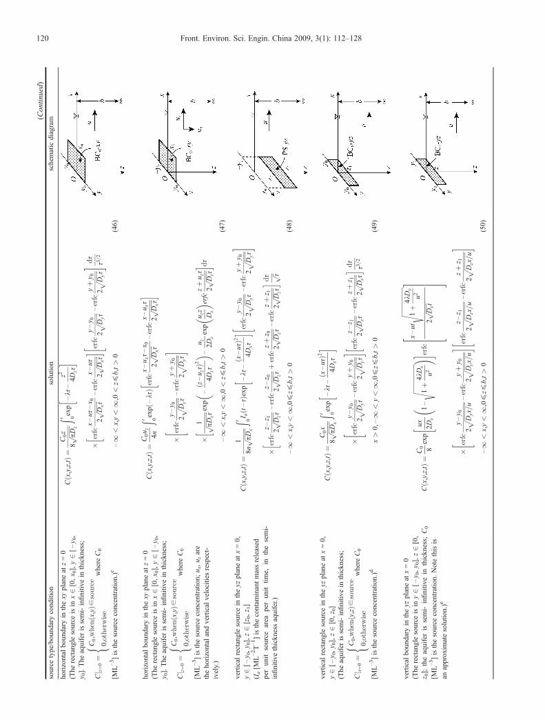
Figure 2 presents a graph of relative concentrations (CD)versus dimensionless time (tD), calculated using Eq. (72),without decay (lD = 0) or sorption (RD = 1) and for differ-ent values of Peclet numbers (Pe). Calculations are per-formed along the plume centerline (yD = 0, zD = 0.5) for asource of coordinates xD0 = 0.5, yD0 = 0.25, zD0 = 0,zD1 = 0.5, and uD = 1. It is found that dimensionless timevalues to reach quasi steady-state conditions are differentfor different Peclet numbers and smaller Peclet numbershave larger dimensionless time values to reach. This is dif-ferent than what was described by Guyonnet and Neville(2004), in which a constant dimensionless time value of 10 issuggested [29]. From Fig. 2 it can be seen that the concen-trations increasewith time for agiven space point. Differentplaces have experienced a similar concentration change.Locations of smaller Peclect numbers (Pe = xD) have longerconcentration increase duration of dimentionless time thanthose of larger ones before they reach their steady state.Figure 3 is the calculation results of Eq. (72) for steady
state concentrations along the x direction for differentvalues of dimensionless lateral distance (yD) with zD keptequal to 0.5 and uD to 1. The calculations are performedwith the same source conditions as in Fig. 2 with yD valuesfrom 0 to 5. As groundwater flows along the x axis and thedimensionless source length is 0.5 in the x direction(Pe0 = xD0), the steady concentrations increase in theplaces of Peclet number from 0 to 3 along the plume cen-terline with the maximum value at the point of Pecletnumber equal to 0.3. Then the concentrations decreaserapidly. The steady concentrations are significantly influ-enced by lateral distance to the plume centerline, espe-cially at low values of Peclet number, but with a similartrend of distributions.
Fig. 2 Type curves of Eq. (72) along the plume centerline for different values of Peclet number (Pe)
Hongtao WANG et al. Solutions library of three-dimensional contaminant transport in uniform flow field in porous media 125

4.2 Effect of source geometries on the concentrations
For a given transport equation, analytical solutions willdiffer according to the source geometry [29]. Huyakorn etal. [31] compared several analytical solutions for three-dimensional transport in groundwater. Guyonnet andNeville [29] compared two solutions: one is the solutionproposed by Domenico [14], as shown in Eq. (50) and theother, by Sagar [21] in Eq. (49). As an example, the effectof three different sources—point, line, and plane on theconcentration calculations will be discussed. The dimen-sionless forms of Eq. (36) for the line source and Eq. (40)for the plane source are
CD ¼ 1
8yD0
ffiffiffiffiffiffiPe
p
s!
tD
0exp – lDPeτ –
Peð1 – τÞ24τ
� �
� erfcyD – yD02ffiffiffiffiffiffiffiPeτ
p – erfcyD þ yD02ffiffiffiffiffiffiffiPeτ
p� �
� 1þ 2X1m¼1
cosmpzD0cosmpzDexp –m2p2
u2DPeτ
� �" #dτffiffiτ
p ,
(73)
and
CD ¼ 1
8yD0ðzD1 – zD0Þ
ffiffiffiffiffiffiPe
p
r!
tD
0exp – lDPeτ –
Peð1 – τÞ24τ
� �
� erfcyD – yD02ffiffiffiffiffiffiffiPeτ
p – erfcyD þ yD02ffiffiffiffiffiffiffiPeτ
p� �
� zD1 – zD0 þ2
p
X1m¼1
1
mðsinmpzD1 – sinmpzD0Þ
"
�cosmpzDexp –m2p2
u2DPeτ
� ��dτffiffiτ
p , (74)
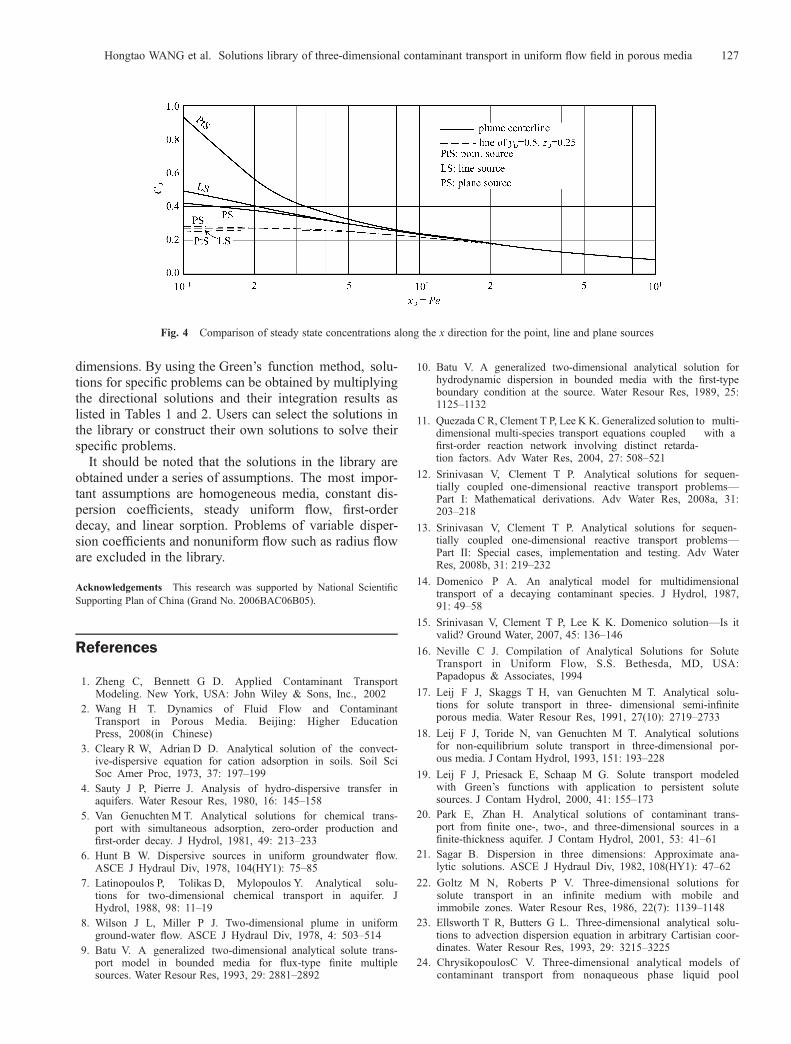
respectively, and the dimensionless form for the pointsource is shown in Eqs (69) and (70). The sources areplaced in the middle of the aquifer thickness with a dimen-sionless length of 1.0 for the line source and side lengths of1.0 � 0.5 for the rectangle plane source. Three types ofsources have the same source strength. The concentra-tions are calculated for the steady state along the plumecenterline and the line of yD = 0.5 and zD = 0.25, as shownin Fig. 4.It is shown that the source types affect the concentra-
tion distribution significantly for smaller values of Pecletnumber. However, this effect decreases with the increasein Peclet number. For the case described above with unitaquifer thickness and isotropic dispersion coefficients, theconcentration difference is less than 5% when the Pecletnumber is greater than 1.0. As the source size gets larger,the medium gets more anisotropic. When the aquifer getsthicker, the effect of source types on concentrationsbecomes greater. Accordingly, the value of Peclet number,beyond which the effect of source types can be neglected,gets larger.
5 Conclusions
The library of analytical solutions presented in this paperis a useful tool to analyze the contaminant transport inporous media. Dimensionless forms of the solutions pro-vided make dimensionless analyses very convenient, suchas drawing type curves and comparing solutions. The cor-rectness of the solutions is well tested by known solutionsand inter-comparison. As the library covers most of theavailable solutions, it can be used to solve a wide range ofcontaminant transport problems for one or multiple
Fig. 3 Steady state concentrations of Eq. (72) along the x direction for different values of dimensionless lateral distance (yD) withzD = 0.5 and uD = 1
126 Front. Environ. Sci. Engin. China 2009, 3(1): 112–128
dimensions. By using the Green’s function method, solu-tions for specific problems can be obtained by multiplyingthe directional solutions and their integration results aslisted in Tables 1 and 2. Users can select the solutions inthe library or construct their own solutions to solve theirspecific problems.It should be noted that the solutions in the library are
obtained under a series of assumptions. The most impor-tant assumptions are homogeneous media, constant dis-persion coefficients, steady uniform flow, first-orderdecay, and linear sorption. Problems of variable disper-sion coefficients and nonuniform flow such as radius floware excluded in the library.
Acknowledgements This research was supported by National ScientificSupporting Plan of China (Grand No. 2006BAC06B05).
References
1. Zheng C, Bennett G D. Applied Contaminant TransportModeling. New York, USA: John Wiley & Sons, Inc., 2002
2. Wang H T. Dynamics of Fluid Flow and ContaminantTransport in Porous Media. Beijing: Higher EducationPress, 2008(in Chinese)
3. Cleary R W, Adrian D D. Analytical solution of the convect-ive-dispersive equation for cation adsorption in soils. Soil SciSoc Amer Proc, 1973, 37: 197–199
4. Sauty J P, Pierre J. Analysis of hydro-dispersive transfer inaquifers. Water Resour Res, 1980, 16: 145–158
5. Van Genuchten M T. Analytical solutions for chemical trans-port with simultaneous adsorption, zero-order production andfirst-order decay. J Hydrol, 1981, 49: 213–233
6. Hunt B W. Dispersive sources in uniform groundwater flow.ASCE J Hydraul Div, 1978, 104(HY1): 75–85
7. Latinopoulos P, Tolikas D, Mylopoulos Y. Analytical solu-tions for two-dimensional chemical transport in aquifer. JHydrol, 1988, 98: 11–19
8. Wilson J L, Miller P J. Two-dimensional plume in uniformground-water flow. ASCE J Hydraul Div, 1978, 4: 503–514
9. Batu V. A generalized two-dimensional analytical solute trans-port model in bounded media for flux-type finite multiplesources. Water Resour Res, 1993, 29: 2881–2892
10. Batu V. A generalized two-dimensional analytical solution forhydrodynamic dispersion in bounded media with the first-typeboundary condition at the source. Water Resour Res, 1989, 25:1125–1132
11. Quezada C R, Clement T P, Lee K K. Generalized solution to multi-dimensional multi-species transport equations coupled with afirst-order reaction network involving distinct retarda-tion factors. Adv Water Res, 2004, 27: 508–521
12. Srinivasan V, Clement T P. Analytical solutions for sequen-tially coupled one-dimensional reactive transport problems—Part I: Mathematical derivations. Adv Water Res, 2008a, 31:203–218
13. Srinivasan V, Clement T P. Analytical solutions for sequen-tially coupled one-dimensional reactive transport problems—Part II: Special cases, implementation and testing. Adv WaterRes, 2008b, 31: 219–232
14. Domenico P A. An analytical model for multidimensionaltransport of a decaying contaminant species. J Hydrol, 1987,91: 49–58
15. Srinivasan V, Clement T P, Lee K K. Domenico solution—Is itvalid? Ground Water, 2007, 45: 136–146
16. Neville C J. Compilation of Analytical Solutions for SoluteTransport in Uniform Flow, S.S. Bethesda, MD, USA:Papadopus & Associates, 1994
17. Leij F J, Skaggs T H, van Genuchten M T. Analytical solu-tions for solute transport in three- dimensional semi-infiniteporous media. Water Resour Res, 1991, 27(10): 2719–2733
18. Leij F J, Toride N, van Genuchten M T. Analytical solutionsfor non-equilibrium solute transport in three-dimensional por-ous media. J Contam Hydrol, 1993, 151: 193–228
19. Leij F J, Priesack E, Schaap M G. Solute transport modeledwith Green’s functions with application to persistent solutesources. J Contam Hydrol, 2000, 41: 155–173
20. Park E, Zhan H. Analytical solutions of contaminant trans-port from finite one-, two-, and three-dimensional sources in afinite-thickness aquifer. J Contam Hydrol, 2001, 53: 41–61
21. Sagar B. Dispersion in three dimensions: Approximate ana-lytic solutions. ASCE J Hydraul Div, 1982, 108(HY1): 47–62
22. Goltz M N, Roberts P V. Three-dimensional solutions forsolute transport in an infinite medium with mobile andimmobile zones. Water Resour Res, 1986, 22(7): 1139–1148
23. Ellsworth T R, Butters G L. Three-dimensional analytical solu-tions to advection dispersion equation in arbitrary Cartisian coor-dinates. Water Resour Res, 1993, 29: 3215–3225
24. ChrysikopoulosC V. Three-dimensional analytical models ofcontaminant transport from nonaqueous phase liquid pool
Fig. 4 Comparison of steady state concentrations along the x direction for the point, line and plane sources
Hongtao WANG et al. Solutions library of three-dimensional contaminant transport in uniform flow field in porous media 127

dissolution in saturated subsurface formations. Water ResourRes, 1995, 31: 1137–1145
25. Sim Y, Chrysikopoulos C V. Analytical solutions for solutetransport in saturated porous media with semi-infinite or finitethickness. Adv Water Res, 1999, 22(5): 507–519
26. Luo J, Cirpka O A, Fienen M N, Wu W M, Mehlhorn T L,Carley J, JardineP M, CriddleC S, KitanidisP K. A parametrictransfer function methodology for analyzing reactive transportin nonuniform flow. J Contam Hydrol, 2006, 83: 27–41
27. Yeh G T, Tsai Y J. Analytical three dimensional transient mod-eling of effluent discharges. Water Resour Res, 1976, 12: 533–540
28. Jones N L, Clement T P, Hansen C M. A three-dimensionalanalytical tool for modeling reactive transport. GroundWater, 2006, 44: 613–617
29. Guyonnet D, Neville C. Dimensionless analysis of two analyt-ical solutions for 3-D solute transport in groundwater. JContam Hydrol, 2004, 75: 141–153
30. Bear J. Dynamics of Fluids in Porous Media. New York,USA: Elsevier, 1972
31. Huyakorn P, Ungs M, Mulkey L, Sudicky E. A three-dimen-sional analytical method for predicting leachate migration.Ground Water, 1987, 25(5): 588–598
128 Front. Environ. Sci. Engin. China 2009, 3(1): 112–128