Analytical Solution of the Diffusivity Equation. FAQReferencesSummaryInfo Learning Objectives Introduction Analytical Solution Linear Systems Radial Systems

Analytical Solution of the Diffusivity Equation

FAQReferenc

esSummar

yInfo

Learning Objectives

Introduction

Analytical SolutionLinear Systems

Radial Systems

Program ExerciseResources

Home

HOMERadial System Linear System

Introduction

Programming Exercise

Resources

Analytical Solution

FAQReferenc

esSummar

yInfo

Learning Objectives

Introduction


Radial Systems


Learning Objectives

Learning objectives in this module:

1. Develop problem solution skills using computers and numerical methods

2. Review flow equations and methods for analytical solution the equations

3. Develop programming skills using FORTRAN

No new FORTRAN elements are introduced in this module, you should, from what you have learnt earlier, be able to solve this problem without any problems

FAQReferenc

esSummar

yInfo

Learning Objectives

Introduction


Radial Systems


Introduction

In analysis of fluid flow in petroleum reservoirs, we need partial differential equations that describe the fluids flowing and the reservoir they are flowing in. Then we need to be able to solve the equations for the conditions of flow that we are interested in. Derivation of the equations normally involves the following elements:

Continuity equations Darcy’s equations PVT relationships for the fluids Compressibility of reservoir rock

Examples of such equations are the simplest forms of the diffusivity equations for linear and radial flow

FAQReferenc

esSummar

yInfo

Learning Objectives

Introduction


Radial Systems


Introduction

Below, the geometries of the two simple reservoir systems and the corresponding partial differential equations are shown:

Q

x=0

x=L

2P

x2(

c

k)Pt

r

1

r

r

(rP

r)

c

k

P

t

Linear flow

Radial flow

FAQReferenc

esSummar

yInfo

Learning Objectives

Introduction


Radial Systems


Analytical Solution

In order to solve the partial differential equations shown earlier, we need to have initial conditions, i.e. initial pressure distribution in the system, and boundary conditions, i.e. rates or pressures at for instance left and right sides of the systems. We will examine two of the most common sets of conditions and analytical solutions for these

Linear System

Radial System

FAQReferenc

esSummar

yInfo

Learning Objectives

Introduction


Radial Systems


Linear System

For the linear system, we have a horizontal porous rod, where fluid is being injected into the left face at a flow rate Q. The injected fluid will be transported through the rod and eventually be produced out of the right face of the rod.

The one-phase partial differential equation (PDE) for this system, in it’s simplest form, is called the linear diffusivity equation. It is valid for one-dimensional flow of a liquid in a horizontal system, where it is assumed that porosity (), viscosity (), permeability (k ) and compressibility (c ) all are constants.

Qin

x=0

x=L

QoutPL

PR

FAQReferenc

esSummar

yInfo

Learning Objectives

Introduction


Radial Systems


Linear System

The linear diffusivity equation may be written as:

(1)

If the initial pressure of the rod is PR , and we assume constant pressures at the end faces, PL and PR for left and right faces, respectively, we have the following analytical solution:

(2)

t

P

k

c

x

P

)(2

2

P(x,t ) PL (PR PL )x

L

2

1

nexp(

n2 2

L2

k

ct )sin(

nx

L)

n 1

Continue

FAQReferenc

esSummar

yInfo

Learning Objectives

Introduction


Radial Systems


which is the expression for a straight line

Linear System

The pressure solution is dependent on position, x, as well as time, t. As time increases, the exponential term becomes smaller, and eventually the solution reduces to the steady-state form:

Click to see what the equation reduces to as time increases

P(x,t ) PL (PR PL )x

L

2

1

nexp(

n2 2

L2

k

ct )sin(

nx

L)

n 1

?

(2)(3)

FAQReferenc

esSummar

yInfo

Learning Objectives

Introduction


Radial Systems


Linear System

The corresponding steady state differential equation is obtained by setting the right hand side of Eq. (1) equal to zero:

Graphically, the solution may be presented as:

d2Pdx2 0

P

x

Left sidepressure

Initial andright sidepressure

Steady statesolution

Transientsolution

As can be observed from the figure, the pressure will increase in all parts of the system for some period of time (transient solution), and eventually approach the final distribution (steady state), described by a straight line between the two end pressures

(4)

FAQReferenc

esSummar

yInfo

Learning Objectives

Introduction


Radial Systems


Radial System

For the radial system below (one-dimensional cylindrical coordinates), we have a horizontal porous disk, where fluid is being injected at the outer boundary and produced at the center. The one-phase one-dimensional (radial) flow equation (PDE) in this coordinate system becomes:

For an infinite reservoir at an initial pressure Pi and with P(r∞)=Pi

and well rate q from a well in the center (at r=rw) the analytical solution is:

where is the exponential integral

1r

r

1rPr

ck

Pr

P Pi q

4khEi

cr 2

4kt

Ei( x) e u

ux

du

(6)

(5)

r rw

Continue

Continue

FAQReferenc

esSummar

yInfo

Learning Objectives

Introduction


Radial Systems


Radial System

A steady state solution does not exist for an infinite system, since the pressure will continue to decrease as long as we produce from the center. However, if we use a different set of boundary conditions, so that:

we can solve the steady state form of the equation:

By integrating twice, the steady state solution becomes:

P(r rw ) Pw

P(r re) Pe

1r

ddr

1r

dPdr

0

P Pw Pe Pw

ln re / rw ln r / rw

(7)

(9)

(8)

Continue

Continue

FAQReferenc

esSummar

yInfo

Learning Objectives

Introduction


Radial Systems


Program Exercise

This programming exercise involves the construction of a reservoir simulation program, although in a very simple form. The following steps should be carried out:

1. Make a FORTRAN program that computes the analytical solutions of Eqs. (2) and (6). When the program is started, it should ask on the screen which geometry should be used, LIN or RAD, and the name of the input data file (where all parameters are to be read from)

2. Read from the screen which values of x (or r) and t the solution should be computed for.

3. The results should be written to the screen as well as to an output file

Data set for linear system

Data set for radial system

Here

Here

FAQReferenc

esSummar

yInfo

Learning Objectives

Introduction


Radial Systems


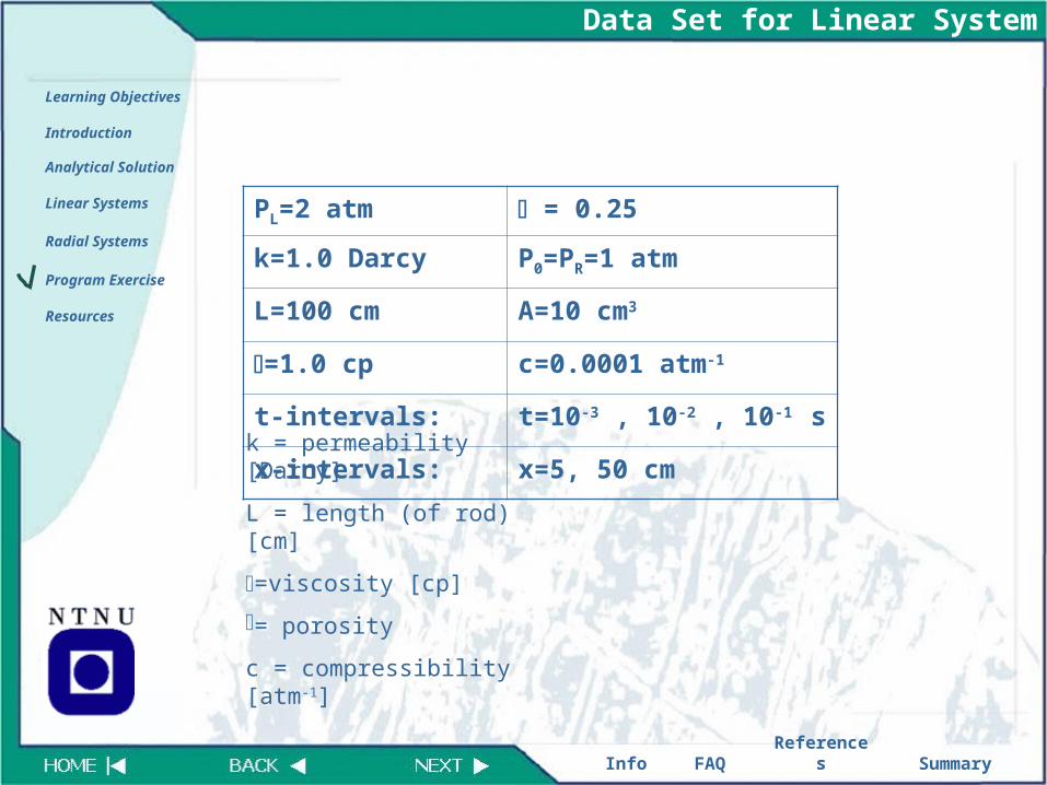
Data Set for Linear System

PL=2 atm = 0.25

k=1.0 Darcy P0=PR=1 atm

L=100 cm A=10 cm3

=1.0 cp c=0.0001 atm-1

t-intervals: t=10-3 , 10-2 , 10-1 s

x-intervals: x=5, 50 cmk = permeability [Darcy]

L = length (of rod) [cm]

=viscosity [cp]

= porosity

c = compressibility [atm-

1]

FAQReferenc

esSummar

yInfo

Learning Objectives

Introduction


Radial Systems


Data Set for Radial System

h=1000 cm = 0.25

k=1.0 Darcy c=0.0001 atm-1

rw=25 cm q=104 cm3/s

=1.0 cp

t-intervals: t= 1E06, 5E06, 10E06 s

r-intervals: r=100, 1000, 5000 cm

k = permeability [Darcy]

rw=wellbore radius [cm]

=viscosity [cp]

= porosity

c = compressibility [atm-

1]

q=flowrate [cm3/s]

FAQReferenc

esSummar

yInfo

Learning Objectives

Introduction


Radial Systems


Resources

Introduction to Fortran

Fortran Template here

The whole exercise in a printable format here

Web sites

Numerical Recipes In Fortran

Fortran Tutorial

Professional Programmer's Guide to Fortran77

Programming in Fortran77

Fortran Template

PDE_Analytical

FAQReferenc

esSummar

yInfo

Learning Objectives

Introduction


Radial Systems


General information

Title: Analytical Solution of the Diffusivity Equation

Teacher(s): Professor Jon Kleppe

Assistant(s): Per Jørgen Dahl Svendsen

Abstract: Provide a good background for solving problems within petroleum related topics using numerical methods

4 keywords: Diffusivity Equation, Linear Flow, Radial Flow, Fortran

Topic discipline:

Level: 2

Prerequisites: None

Learning goals: Develop problem solution skills using computers and numerical methods

Size in megabytes: 0.7 MB

Software requirements: MS Power Point 2002 or later, Flash Player 6.0

Estimated time to complete:

Copyright information: The author has copyright to the module and use of the content must be in agreement with the responsible author or in agreement with http://www.learningjournals.net.

About the author

Thor A. Thorsen

incling sound, video, animation files

Thor A. Thorsen

for example Geophysics -> Processing

Thor A. Thorsen

0 is very easy – 4 is most difficult

Thor A. Thorsen

in minutes

Thor A. Thorsen

Individual learning or project-based learning

Thor A. Thorsen

Title with reference to version number starting with 1.0

Thor A. Thorsen

Flash-player, etc.

Thor A. Thorsen

With link to an web-site with contact information, taks and publications

Jonny Hesthammer

Ideally, this link should be to the authors web homepage as this will ensure continuous update of adresses, publications etc. However, for those who have not yet created their own homepage we provide a separate page in this document for author information. The current link is to that page and it must be changed (right click with mouse on action button and select "edit hyperlink") to the relevant web link.

FAQReferenc

esSummar

yInfo

Learning Objectives

Introduction


Radial Systems


FAQ

No questions have been posted yet. However, when questions are asked they will be posted here.

Remember, if something is unclear to you, it is a good chance that there are more people that have the same question

For more general questions and definitions try these

Dataleksikon

Webopedia

Schlumberger Oilfield Glossary

FAQReferenc

esSummar

yInfo

Learning Objectives

Introduction


Radial Systems


References

See for instance:H. S. Carslaw and J. C. Jaeger: Conduction of Heat in Solids, 2nd ed., Oxford, 1985

Numerical Recipes in Fortran in pdf format online:

Numerical Recipes in Fortran

FAQReferenc

esSummar

yInfo

Learning Objectives

Introduction


Radial Systems


Summary

Subsequent to this module you should...

be able to keep track of loops and conditional statements

have no problems handling output and input data have obtained a better understanding on solving

problems in Fortran

Documents

Analytical Solution of the Diffusivity Equation. FAQReferencesSummaryInfo Learning Objectives Introduction Analytical Solution Linear Systems Radial Systems