Analytical parameterization of rotors and proof of a Goldberg

Conjecture by Optimal Control Theory

Terence Bayen ∗

Resume

Curves which can be rotated freely in a n-gon (that is a regular polygon with n

sides) so that they always remain in contact with every side of the n-gon are cal-led rotors. Using optimal control theory, we prove that, the rotor with minimal areaconsists of a finite union of arcs of circle. Moreover, the radii of these arcs are exactlythe distances of the diagonals of the n-gon from the parallel sides. Finally, using theextension of Noether’s Theorem to optimal control (as performed in [29]), we showthat a minimizer is necessarily a regular rotor, which proves a conjecture formulatedin 1957 by Goldberg (see [14]).

1 Introduction

In this paper, we investigate properties of rotors, that is, convex curves that can befreely rotated inside a regular polygon Pn with n sides, n ≥ 3, while remaining in contactwith every side of Pn. When n = 4, P4 is a square of side α, and a rotor of P4 is called acurve of constant width α or an orbiform. When n = 3, P3 is an equilateral triangle, anda rotor of P3 is called a ∆-curve. There are infinitely many such curves besides the circle(see section 2).

Orbiforms have been studied geometrically since the nineteen century (see [5], [21],[23], [26], [33]). In particular, Reuleaux’s name is attached to those orbiforms obtained byintersecting a finite number of discs of equal radii α. The Reuleaux triangle is the mostfamous of these orbiforms : it consists of the intersection of three circles of radius one andwhose centers are on the vertices of an equilateral triangle of side one. Orbiforms havemany interesting properties and applications in mechanics (see [5], [6], [7], [22], [23], [24],[33]). For example, Reuleaux triangles are used in boring square holes and it is also partof the Wankel engine used by Japan’s Mazda cars ( c©Copyright Mazda Motor Corpora-tion). Nowdays, the study of rotors is potentially interesting in mechanics for the designof engines or propellers in the navy for example.

An interesting shape optimization problem consists in determining the convex bodymaximizing or minimizing the area in the class of rotors. It is easy to show that the disc hasalways maximal area in this class. This is a consequence of the isoperimetric inequality asall rotors have the same perimeter (see Barbier’s Theorem in section 2.3). The question offinding a rotor of least area is more difficult. First, notice that the problem of minimizing

∗Laboratoire des Signaux et Systemes, Ecole Superieure d’Electricite, 91192 Gif-sur-Yvette, France.bayen@ann.jussieu.fr, http://www.cmap.polytechnique.fr/~bayen/

1

the area is well posed, as rotors are convex bodies (see section 2.2). This question has beensolved for n = 4 (that is in the case of orbiforms) by Blaschke using the mixed-volume(see [5]) and Lebesgue (see [21]). They show that the Reuleaux triangle has the least areain the class of constant width bodies of R

2. Fujiwara has given the first analytic proof ofthis result (see [11]). More recently, Harrell gave a modern proof using minimization underconstraints (see [17]). The study of these problems in R

2 is useful for extensions in R3, and

also in the domain of spectral analysis. For example, the problem of finding a constantwidth body of minimal volume in R

3 has been recently investigated (see [4], [19]). Theoptimization of eigenvalues with respect to the domain Ω is also an intense field of research(see [18] for an overview of many spectral problems involving convexity). These questionsrequire a careful study of the dimension 2.

The ∆-curves have many similar geometrical properties to the orbiforms (see [7], [33]).Fujiwara gave an analytic proof in [11] that, among all ∆-curves inscribed in an equilateraltriangle of side one, the one of minimal area is the ∆-biangle or lens. It consists of two

circular arcs of radius√

32 and of length π

3 . This result was also established by Blaschkeand later by Weissbach (see [32]).

Whereas the case n = 3 and n = 4 have been investigated, the question of findingthe rotor of least area for n ≥ 5 is open. Standard geometrical proofs cannot be appliedin this case (see [12]). In [14] and [15], Goldberg constructs a family of ”trammel” rotorsin a regular polygon, (Oln±1

n )l∈N∗ , that have 2(ln± 1) symmetries, and he conjectured in[14] that the minimizer is a rotor called On−1

n obtained for l = 1. The boundary of a rotorOln±1

n consists of a finite union of arcs of circles of different radii ri and of equal sectors (seesection 2.6). The values ri are exactly the distances of the diagonals of the n-gon from theparallel sides. In this class, On−1

n has the minimum number of arcs. An analytic descriptionof these regular rotors is given in [10] by Focke. In 1975, Klotzler made an analytic studyof the minimization problem using optimal control theory (see [2], [3], [20]). He showed in[20] that a minimizer consists of a union of arcs of circle of radii ri, but he failed to provethat a minimizer is in the class (Oln±1

n )l∈N∗ . His idea consists in reformulating the initialminimization problem into an optimal control problem by choosing the radius of curvatureas control variable. Unfortunately, he seems to prove that the regular rotors Oln±1

n are localminimizers of the area in the subclass Rln±1

n of rotors having the same number of arcs andthe same radii of curvature. This result contradicts the one of Firey (see [9]) in the casen = 4 : the author shows that regular Reuleaux polygons with N sides, N ≥ 5, maximizethe area in the class of Reuleaux polygons with the same number of sides. Moreover, in[2], the author performs only convex perturbations of a regular rotor Oln±1

n . This kindof perturbation increases the area by the concavity of the functional (Brunn-Minkowski’sTheorem, see [8]). The main difficulty is to consider non-convex perturbations of thoserotors which are not obtained by a strictly convex combination of two rotors.

The aim of the paper is to prove the following theorem conjectured by Goldberg in1957 (see [14]) :

Theorem 1.1 Among all rotors of a regular polygon Pn (n ≥ 3), the one of minimal areais the regular rotor On−1

n .

In section 2, we give an analytic parameterization of a rotor using the support function ofa convex body (see [6] or [27], for an overview of the properties of the support function). Insection 3, we formulate the minimization problem into an optimal control problem which

2

is similar to the one obtained by Klotzler (see [20]). Indeed, the convexity constraintsenable us to choose the radius of curvature of the boundary of a rotor, as control variable.Thanks to this new parameterization, the initial shape optimization is well posed. Bythe Pontryagin Maximum Principle (PMP), we show that the extremal trajectories are”bang-bang” and we determine the corresponding number of switching points. We thusrestrict the class of extremal trajectories step by step. Whereas the computation of theextremal trajectories performed by Klotzler, is incomplete (he does not show that theswitching points of an extremal trajectory are equidistant), we prove, in section 4, Theorem1.1 by using an extension of Noether’s Theorem to optimal control theory provided in[28]. We compute conserved quantities along an extremal trajectory, and thus, we cancharacterize the switching points of an extremal (see section 4). This shows that therotors corresponding to the extremal trajectories belong to the class (Oln±1

n )l∈N∗ . Wethen conclude the proof of Goldberg’s conjecture by proposition 2.11. Note that by thisproposition, there is no need to examine the optimality of extremal trajectories.

2 Construction of a rotor

2.1 Support function of a convex body

A body or a domain in RN ,N ≥ 2, is a non-empty compact connected subset of R

N . LetK be a convex body. The support function of K is defined as the map hK : R

N\0 → R

withhK(ν) := max

x∈Kx · ν, ν ∈ R

N\0.

The support function is clearly homogeneous of degree 1. A convex body is uniquelydetermined by its support function (see [6] p.29 or [19]). Let K be a convex body of non-empty interior and assume that the origin is inside K. Recall that, for a convex body, ahyperplane H is a hyperplane of support for K if there exists x ∈ K ∩ H such that Kis included in one of the half-spaces defined by H. If ν belongs to SN−1, hK(ν) can beinterpreted as the distance from the origin to the support hyperplane of K with normalvector ν (see figure 1). The support function is non negative if and only if the originis inside K. The next proposition characterizes the degree of regularity of the supportfunction (see [6] p.28 or [27]) :

Proposition 2.1 Let K be a convex body of RN and hK its support function. Then hK

is of class C1 if and only if K is strictly convex.

From now on, we consider convex bodies in dimension 2. The support function of aconvex body K of R

2 will be denoted pK(θ) := hK(eiθ), θ ∈ R or p(θ) to simplify. Thefunction pK is 2π-periodic. If K is a convex body, we denote by ∂K its boundary. Given(z1, z2) ∈ C

2, their scalar product in R2 will be written indifferently ℜ(z1z2) or z1 · z2.

Proposition 2.2 Let K be a strictly convex body and p its support function. We assumethat the boundary of K, ∂K is Lipschitz. Then, ∂K can be described by the equations :

x(θ) = p(θ) cos(θ) − p(θ) sin(θ),

y(θ) = p(θ) sin(θ) + p(θ) cos(θ),(2.1)

where θ ∈ R.

3

Fig. 1 – The support function of a convex body K is the distance p(θ) between the tangentto K orthogonal to (cos(θ), sin(θ)) and the origin.

Proof. Let θ be in [0, 2π] and uθ the vector of coordinates (cos(θ), sin(θ)). The supportfunction p(θ) is defined by :

p(θ) := maxx∈K

x · uθ,

and p is of class C1 by the strict convexity. As K is compact, the maximum is reached atsome point of coordinates (x(θ), y(θ)) and we have :

x(θ) cos(θ) + y(θ) sin(θ) = p(θ). (2.2)

As the boundary of K is Lipschitz, the functions (x, y) are differentiable almost everywhere(Rademacher’s Theorem). Moreover, the vector uθ is orthogonal to the support line givenby X cos(θ) + Y sin(θ) = 0, hence, we must have :

(x(θ), y(θ)) · ~uθ = 0.

By derivating (2.2), we get :

−x(θ) sin(θ) + y(θ) cos(θ) = p(θ),

which gives (2.1).

Equation (2.1) can be rewritten : z(θ) := x(θ) + iy(θ) = (p(θ) + ip(θ))eiθ.

In the following, the space C1,1 denotes the set of maps p : R → R, of class C1, andsuch that p is locally Lipschitz.

Proposition 2.3 Let K be a convex body and p its support function. We assume that pis of class C1,1. Then, the radius of curvature p + p of the boundary ∂K exists almosteverywhere and, for a.e. θ ∈ R,

p(θ) + p(θ) ≥ 0. (2.3)

Proof. As p is of class C1,1, the functions (x(θ), y(θ)) are differentiable almost everywhereand by standard formulas, the radius of curvature f of ∂K is given by f = p+ p. As thebody K is convex, f must be non negative and consequently we have f(θ) = p(θ)+p(θ) ≥ 0for a.e. θ ∈ R.

If K is a convex body of support function p and if p is of class C1,1, the tangent vec-tor to ∂K is given by

z(θ) = i(p(θ) + p(θ))eiθ.

4

When p + p = 0 on a set A of positive measure, then we have z = 0. Geometricallyspeaking, this means that the boundary ∂K has a corner : for θ ∈ A, the point z(θ) isstationary. For a given function f ∈ L∞(R,R) and 2π-periodic, we denote by

c1(f) =1

2π

∫ 2π

0f(θ)eiθdθ,

the first Fourier coefficient of f .

Proposition 2.4 Let f ∈ L∞(R,R) be a 2π-periodic function. Then, any function p thatsatisfies f = p+ p is of class C1,1, and p is 2π-periodic if and only if c1(f) = 0.

Proof. Let f ∈ L∞(R,R) be a 2π-periodic function. A function p satisfies f = p + p ifand only if there exists (a, b) ∈ R

2 such that for all θ ∈ R :

p(θ) =

∫ θ

0f(t) sin(θ − t)dt+ a cos(θ) + b sin(θ). (2.4)

By (2.4), any function p that satisfies p + p = f is of class C1,1. Moreover, any suchfunction p is of class C1,1, and is 2π-periodic if and only if its restriction on [0, 2π] satisfiesp(0) = p(2π), p(0) = p(2π). But we have :

∫ 2π

0(p(θ) + p(θ))eiθdθ = p(2π) − p(0) − i(p(2π) − p(0)).

Hence, any function p satisfying (2.4) is 2π-periodic if and only if p(2π) = p(0) andp(2π) = p(0), that is if and only if c1(f) = 0.

If we deal with f = p+ p instead of p, we get an additional condition c1(f) = 0 which saysthat the boundary ∂K given by equation (2.1) is closed. The next theorem is a consequenceof the two previous propositions.

Theorem 2.1 (i). Let K be a strictly convex body of R2 and p its support function. If p

is of class C1,1, then p+ p ≥ 0.(ii). Conversely, let f ∈ L∞(R,R) be a 2π-periodic function such that f ≥ 0 and c1(f) = 0.If p is a function satisfying f = p+ p, then p is of class C1,1, 2π-periodic (in the sense ofC1,1 maps) and it is the support function of a strictly convex body.

Let K be a strictly convex body. We denote by p its support function of class C1 and byA(p) its area. By Stokes’s formula and by (2.1), we have :

A(p) =1

2

∫ 2π

0(p2(θ) − p2(θ))dθ. (2.5)

By integrating by parts, the area becomes :

A(p) =1

2

∫ 2π

0p(θ)

(

p(θ) + p(θ))

dθ, (2.6)

which has a sense because p+ p is a positive Radon measure, and (2.6) can be interpretedas the product of a positive Radon measure and a continuous function. In the next section,we show that the support function of a rotor is of class C1,1 and (2.6) is clearly defined inthat case.

5

2.2 Construction of a rotor by its support function

In this section, we recall classical definitions and properties of rotors (see [6],[16],[33]).Let K be a convex domain and P be a convex polygon. P will be called a tangential

polygon of K and K an osculating domain in P , if K ⊂ P and every side of P has anon-empty intersection with K (see [16]). We say that a polygon P is equiangular if allits interior angles at the vertices are equal. We say that a convex polygon P is a n-gon ifit is a regular polygon with n sides, n ≥ 3.

Definition 2.1 A convex domain K will be called a rotor in a polygon Q if for everyrotation ρ, there exists a translation vector pρ such that ρK + pρ is an osculating domainin K.

In the following, we assume that Q is a regular polygon with n ≥ 3 sides, that is weconsider only rotors of a regular polygon. Hence, K is a rotor in a regular n-gon Q if andonly if all tangential equiangular n-gons are regular and have equal perimeters. A rotor ofa n-gon Pn has the property to rotate inside Pn while remaining in contact with all sidesof Pn. The disc is the most simple example of rotor. A rotor is a strictly convex domain(see [16],[33]). Consequently the support function of a rotor is of class C1.

Let r be the radius of the inscribed circle of the n-gon Pn and δ := 2πn . We give in

the following theorem an analytic description of a rotor which will be used in the rest ofthe paper.

Theorem 2.2 (i). Let K be a rotor and p its support function. Then, p satisfies :

p(θ) − 2 cos(δ)p(θ + δ) + p(θ + 2δ) = 4r sin2

(

δ

2

)

, ∀θ ∈ [0, 2π]. (2.7)

Moreover p is of class C1,1 and satisfies (2.3).(ii). Conversely, let p be a 2π-periodic function of class C1,1. Assume that p satisfies (2.3)and (2.7). Then p is the support function of a rotor K.

The characterization of a rotor by (2.7) is well-known (see [7], [10], [20]), but we show inparticular that the support function of a rotor is actually of class C1,1. Before doing theproof of the theorem, we set some notations :

Sn(p) := p(θ) − 2 cos(δ)p(θ + δ) + p(θ + 2δ), (2.8)

and

Cn := 4r sin2

(

δ

2

)

. (2.9)

Proof of (i). We refer to chapter 8 of [33] for the following geometric property. Bydefinition of a rotor, the tangents to ∂K at each contact point are the sides of the n-gon.Hence the perpendiculars to these paths at their contact points meet in a point which isthe instantaneous center of rotation of the body. A simple computation yields (2.7). Wenow prove that p is of class C1,1. First, we have :

∑

0≤k≤n−1

p(θ + kδ) = nr, ∀θ ∈ R. (2.10)

Indeed, by writing (2.7) at points θ, θ + δ,...,θ + (n − 1)δ, and adding all this equalities,we get (2.10). As K is strictly convex, its support function p is of class C1. We now showthat p satisfies the inequality :

(

p(θ′) − p(θ))

sin(θ − θ′) ≤(

p(θ) + p(θ′)) (

1 − cos(θ − θ′))

, ∀(θ, θ′) ∈ [0, 2π]. (2.11)

6

By definition of the support function, we have for all (θ, θ′) ∈ [0, 2π] :

(x(θ′), y(θ′)) · (cos(θ), sin(θ)) ≤ p(θ).

Taking into account (2.1), we get :

p(θ′) sin(θ − θ′) ≤ p(θ) − p(θ′) cos(θ′ − θ).

If we permute θ and θ′, we obtain :

p(θ) sin(θ′ − θ) ≤ p(θ′) − p(θ) cos(θ′ − θ).

Adding the two last inequalities yields (2.11). We now write (2.11) at the points θ + kδ

and θ′ + kδ, 0 ≤ k ≤ n− 1. We get, for all (θ, θ′) ∈ [0, 2π] and 0 ≤ k ≤ n− 1,

(

p(θ′ + kδ) − p(θ + kδ))

sin(θ − θ′) ≤(

p(θ + kδ) + p(θ′ + kδ)) (

1 − cos(θ − θ′))

. (2.12)

By (2.10), we obtain for all (θ, θ′) ∈ [0, 2π] :

∑

1≤k≤n−1

p(θ + kδ) = nr − p(θ), (2.13)

and∑

1≤k≤n−1

p(θ + kδ) = −p(θ). (2.14)

Combining (2.12), (2.13) and (2.14), we obtain :

(

−p(θ′) + p(θ))

sin(θ − θ′) ≤ (2nr − p(θ) − p(θ′))(1 − cos(θ − θ′)).

Therefore, by (2.11) and the previous inequality, we get for all (θ, θ′) ∈ [0, 2π] :

|(p(θ′) − p(θ)) sin(θ − θ′)| ≤ 2nr sin2

(

θ − θ′

2

)

.

Consequently, p satisfies the inequality :

|p(θ′) − p(θ)| ≤ 2nr

∣

∣

∣

∣

tan

(

θ − θ′

2

)∣

∣

∣

∣

,

for all (θ, θ′) ∈ [0, 2π] such that |θ − θ′| 6∈ 0, π, 2π. This inequality proves that p is Lip-schitz, and thus p is of class C1,1. As K is convex and p of class C1,1, it satisfies (2.3).This concludes the proof of (i).

Proof of (ii). Let us assume that conditions (2.3) and (2.7) are satisfied. As p is of classC1,1, 2π-periodic and satisfies (2.3), it is the support function of a strictly convex bodyK. A straightforward computation using (2.7) shows that an osculating polygon to K isequiangular, consequently, K is a rotor.

An example of a function p satisfying (2.7) is given by :

p(θ) = 1 +1

1 − (ln− 1)2cos((ln− 1)θ) (2.15)

where l ∈ N∗ (see figure 2). A simple computation shows that we have Sn(p) = Cn with

r = 1. Moreover, we have easily p(θ) + p(θ) = 1 + cos((ln− 1)θ) ≥ 0, ∀θ ∈ R. Hence, p is

7

Fig. 2 – Example of rotors whose support function is given by (2.15) for n = 3, l = 2 andn = 5, l = 1, 2.

the support function of a rotor K in a n-gon. The boundary of K is of class C∞ becausep is of class C∞.

In the following, we denote by E the set of the functions p ∈ C1,1(R) that are 2π-periodicand that satisfy (2.3) and (2.7). The problem of finding a rotor of minimal area is nowequivalent to the optimization problem :

minp∈E

A(p). (2.16)

The existence of a minimizer for problem (2.16) follows easily from standard compacityarguments (see [31],[33]).

2.3 Basic properties of rotors

This section is devoted to well-known results about rotors which can be found in thecase n = 3 or n = 4 in [5], [7] and [33]. Let us first recall Barbier’s Theorem which is asimple consequence of (2.7).

Theorem 2.3 Let r be the radius of the inscribed circle in Pn. Then the perimeter ofevery rotor R of Pn is equal to 2πr.

Proof. Let R be a rotor and p be its support function. The perimeter L of R is givenby the integral of the radius of curvature :

L =

∫ 2π

0(p(θ) + p(θ))dθ,

which is well defined as p is of class C1,1. As p is 2π-periodic, the perimeter becomesL =

∫ 2π0 p(θ)dθ. Now, integrating (2.7) on the interval [0, 2π] and using the 2π-periodicity

of p, we get L = 2πr.

Proposition 2.5 Among all rotors of a regular polygon Pn, the one of maximal area isthe disc of radius r.

Proof. By the isoperimetric inequality, the body of maximal area among all closed curveshaving the same perimeter is the disc, and the disc is a rotor of Pn.

When n = 4, a rotor is called a constant width body.

8

Definition 2.2 The width of a convex curve in a given direction is the distance between apair of supporting lines of the curve perpendicular to this direction. If the width is constantin every direction, the curve is a curve of constant width.

Equivalently, a constant width body has the property to rotate inside a square whileremaining tangent to the four sides of the square. The relation (2.7) can be simplified inthe case n = 4, which corresponds to the constant width bodies. The support function ofK satisfies in this case :

p(θ) + p(θ + π) = 2r, ∀θ ∈ R, (2.17)

which is exactly saying that any pair of parallel support lines to K are separated by thedistance 2r (see [13]).

2.4 Formulation of the constraints on the interval [0, 2δ]

In this section, we derive consequences of (2.7) which will be useful to formulate theoptimal control problem associated to the minimization problem. Let us define the realssk and tk for k = 0, ..., n− 1 by :

sk :=sin(kδ)

sin(δ), tk := 2

sin(kδ2 ) sin( (k−1)δ

2 )

cos( δ2)

r. (2.18)

Lemma 2.1 Let p be a map in C1,1(R), 2π-periodic satisfying (2.7). Then we have,

p(θ + kδ) = skp(θ + δ) − sk−1p(θ) + tk, ∀θ ∈ [0, 2π]. (2.19)

Proof. Let θ ∈ [0, 2π] and vk := p(θ + kδ). We have by (2.7) :

vk − 2 cos(δ)vk+1 + vk+2 = 4r sin2

(

δ

2

)

. (2.20)

We solve this linear recurrent sequence and get :

vk = aωk + aωk + r,

where ω := eiδ and v0 = p(θ), v1 = p(θ + δ). This gives (2.19).

Corollary 2.1 If n is even, a rotor K in a n-gon is a constant width body.

Proof. Let K be a rotor and p be its support function which satisfies (2.7). We assumethat n = 2m, m ∈ N

∗. Using (2.19) with k = m, we get sm = 0, sm−1 = 1 and tm = 2r.Consequently, p satisfies :

p(θ +mδ) = −p(θ) + 2r,

which is exactly saying that K is of constant width as mδ = π.

We reformulate now the area of a rotor on the interval [0, 2δ]. Let r be the radius ofthe inscribed circle to the n-gon and P ∈ C1,1(R,R), F ∈ L∞(R,R) be the maps definedby :

P (θ) := p(θ) − r,

F (θ) := p(θ) + p(θ) − r = P (θ) + P (θ).(2.21)

9

Lemma 2.2 Let p be the support function of a rotor and f its radius of curvature. Thearea of a rotor is given by

A(p) =n

4 sin2( δ2)A(P ) + πr2,

where

A(P ) =

∫ δ

0

(

P (θ)F (θ)+P (θ+δ)F (θ+δ)−cos(δ)(

F (θ)P (θ+δ)+F (θ+δ)P (θ))

)

dθ. (2.22)

Proof. We have by (2.6) :

A(f) =1

2

∫ 2π

0p(θ)f(θ)dθ =

1

2

∑

0≤k≤n−1

∫ (k+1)δ

kδp(θ)f(θ)dθ

=1

2

∑

0≤k≤n−1

∫ δ

0p(θ + kδ)f(θ + kδ)dθ.

Replacing p(θ + kδ) and f(θ + kδ) using (2.19), we get the result by the equalities :

∑

0≤k≤n−1

s2k =∑

0≤k≤n−1

s2k−1 =2

2 sin2(δ),

and∑

0≤k≤n−1

sktk = −n

4 cos2( δ2),

∑

0≤k≤n−1

sksk−1 =n cos(δ)

2 sin2(δ).

Note that in the special case of sets of constant width (n = 4), one finds the usualfunctional (see [13]) :

A(p) = πr2 −

∫ π

0p(θ)(1 − f(θ))dθ, (2.23)

which can be easily obtained by (2.6) and (2.17).

2.5 Simplification of the functional

Before going into details for solving the minimization problem (2.16), we diagonalizethe functional (2.22) (see [20] for the same parameterization). In particular, we establishthe equivalence between the parameterization of a rotor by its support function and thenew parameterization. The following parameterization will be useful to define an optimalcontrol problem equivalent to (2.16). We set :

γ := cos(δ), σ := sin(δ), ω1

2 := eiδ2 , ω− 1

2 := e−iδ2 ,

that is we denote by ω1

2 and ω− 1

2 a squareroot of ω and ω.Recall that given a rotor K of support function p, the functions P and F are defined

by (2.21) and by (2.8) and (2.9) we have Sn(f) = Cn if and only if Sn(F ) = 0. We definenow the functions W ∈ C1,1(R,C) and Z ∈ L∞(R,C) by :

W (θ) := P (θ) − ωP (θ + δ),

Z(θ) := F (θ) − ωF (θ + δ),(2.24)

10

where θ ∈ R, so that :W + W = Z. (2.25)

The functions W and Z can be interpreted as the complex support function and thecomplex radius of curvature associated to a rotor. We denote by X1, X3, U , V thereal and imaginary parts of W and Z :

W = X1 + iX3,

Z = U + iV,

so that we have

X1(θ) = P (θ) − γP (θ + δ),

X3(θ) = σP (θ + δ),

U(θ) = F (θ) − γF (θ + δ),

V (θ) = σF (θ + δ).

(2.26)

We have equivalently

P (θ) = X1(θ) + γσX3(θ),

P (θ + δ) = 1σX3(θ),

F (θ) = U(θ) + γσV (θ),

F (θ + δ) = 1σV (θ + δ).

(2.27)

Proposition 2.6 The functions W and Z satisfy the relations :

W (θ + δ) = ωW (θ),∀θ ∈ R,

Z(θ + δ) = ωZ(θ), a.e. θ ∈ R.(2.28)

Proof. Let p be the support function of a rotor. We have by (2.7) Sn(p) = Cn, whereCn is given by (2.9). Thus, Sn(P ) = 0, that is :

∀θ ∈ R, P (θ) − 2γP (θ + δ) + P (θ + 2δ) = 0. (2.29)

Eliminating P (θ + 2δ) in the equation above, we get

∀θ ∈ R, W (θ + δ) = P (θ + δ) − ω(2γP (θ + δ) − P (θ)),

which gives W (θ + δ) = ωW (θ), ∀θ ∈ R. By derivating the previous equation, we getZ(θ + δ) = ωZ(θ), ∀θ ∈ R.

In the following, Pn denotes the regular polygon of center the origin and of vertices thepoints of coordinates (r∗ωkeiα)0≤k≤n−1, where r∗ := 2r sin( δ

2) and α := −π2 − δ

2 .

Proposition 2.7 Let K be a rotor, p its support function and f = p + p its radius ofcurvature. We denote by Z its complex radius of curvature. Then, we have f ≥ 0 if andonly if Z(θ) ∈ Pn, for a.e. θ ∈ [0, δ].

Proof. Let us consider for 0 ≤ k ≤ n− 1 the map defined by

uk(x, y) = sky − sk−1x+ tk.

By Lemma 2.1, we have for θ ∈ [0, δ] and for 0 ≤ k ≤ n− 1 :

f(θ + kδ) = uk (f(θ), f(θ + δ)) .

11

Therefore we have for θ ∈ [0, δ] :

f ≥ 0 ⇐⇒ uk(f(θ), f(θ + δ)) ≥ 0, k = 0, ..., n− 1

⇐⇒ sk

(

f(θ + δ) − r)

− sk−1

(

f(θ) − r)

+ tk + r(sk − sk−1) ≥ 0

⇐⇒ sin(kδ)F (θ + δ) − sin((k − 1)δ)F (θ) ≥ −σr

⇐⇒ ℑ(

sin(kδ)Z(θ) − sin((k − 1)δ)Z(θ − δ))

≥ −σ2r

⇐⇒ ℑ(

sin(kδ)Z(θ) − sin((k − 1)δ)ωZ(θ))

≥ −σ2r

⇐⇒ ℑ(ωk−1Z(θ)) ≥ −σr.

Let z = x+ iy be a complex number, Dk the hyperplane of equation ℑ(ωk−1z) = −σr andHk the half plane defined for z ∈ C by ℑ(ωk−1z) ≥ −σr. We easily have that z ∈ Dk+1 ifand only if ωz ∈ Dk. Hence, for θ ∈ [0, δ], Z(θ) satisfies ℑ(ωk−1Z(θ)) ≥ −σr, 0 ≤ k ≤ n−1if and only if Z(θ) belongs to the intersection of the half spaces Hk. This intersection isnon-empty as 0 belongs toHk for all 0 ≤ k ≤ n−1 and is convex as allHk are convex, henceit is a non-empty convex polygon. Moreover, a simple computation yields that the verticesof Pn are given by the intersection Dk ∩Dk+1 and are of coordinates −2ir sin( δ

2)ei(k−1

2)δ,

for 0 ≤ k ≤ n− 1.

It is convenient to work with Pn because we will see in the next section that the op-timal control takes its values at the vertices of Pn (the extremal points of Pn).

Proposition 2.8 Let p be the support function of a rotor K. Then, the area of K is givenby :

A(p) = πr2 +n

4σ2

∫ δ

0UX1 + V X3 = πr2 +

n

4σ2

∫ δ

0ℜ(ZW ). (2.30)

Proof. The area of the rotor K described by p ∈ E is given by (2.22). Replacing P (θ),P (θ + δ), F (θ) and F (θ + δ) by W (θ), W (θ + δ), Z(θ), Z(θ + δ), we get (2.30) by using(2.28).

Notice the similarity between (2.6) and (2.30).

Definition 2.3 Let Γ be the set of the complex functions W in C1,1([0, δ]) that satisfy :

W (δ) = ωW (0),

W (δ) = ωW (0),(2.31)

and such that the function Z = W + W takes its values in the polygon Pn.

Definition 2.4 We denote by Z the set of the complex valued functions Z ∈ L∞(R,C)satisfying :

Z(θ + δ) = ωZ(θ), ∀ θ ∈ R,

andZ(θ) ∈ Pn, ∀ θ ∈ R.

We can now prove the equivalence between the parameterization of a rotorK by its supportfunction p and its complex support function W .

12

Theorem 2.4 (i). Let W = X1 + iX3 be a function in Γ. Let us define the function p on[0, 2δ] by p = P + r where P is given by (2.27). Then, if we extend p on the interval [0, 2π]by (2.19) and if we note p this extension, p is the support function of a rotor.(ii). Conversely, if p is the support function of a rotor K and P := p−r, then the functionW|[0,δ] defined by (2.24) belongs to Γ.

Proof of (i). First, let us take W = X1 + iX3 ∈ Γ. We have by (2.31) :

1σX3(0) = X1(δ) + γ

σX3(δ),

σX1(0) − γX3(0) = −X3(δ),(2.32)

and

1σ X3(0) = X1(δ) + γ

σ X3(δ),

σX1(0) − γX3(0) = −X3(δ).(2.33)

We now define a function P on the interval [0, 2δ] by :

P (θ) = X1(θ) +γ

σX3(θ), P (θ + δ) =

1

σX3(θ),

for θ ∈ [0, δ]. By (2.32), we have

P(

δ−)

= P(

δ+)

,

and by (2.33) we haveP

(

δ−)

= P(

δ+)

.

Consequently, the function P is of class C1 on [0, 2δ]. By (2.32) we get also

Sn(P )(0) = 0,

and by (2.33) we getSn(P )(0) = 0.

Hence, the functions P and P satisfy Sn(P ) = 0 and Sn(P ) = 0 for θ = 0. If we extendp = P + r to the interval [0, 2π] by (2.19) and to R by 2π-periodicity, it satisfies, byconstruction, Sn(p) = Cn. We also have p(0) = p(2π) and p(0) = p(2π) by (2.19) so thatthe function p is of class C1. Finally, we have p+ p ≥ 0 because Z ∈ Pn. We conclude thatp is the support function of a rotor.

Proof of (ii). Let us now consider the support function p of a rotor. We define a func-tion W by (2.24). First, the condition (2.3) satisfied by p implies that Z = W + W takesits value in Pn. Let us show that W satisfies (2.31). By (2.26), we have :

1

σX3(0) = X1(δ) +

γ

σX3(δ),

and by using Sn(P )(0) = 0, we get :

σX1(0) − γX3(0) = −X3(δ).

These two real conditions implyW (δ) = ωW (0). By using (2.27) and the equality Sn(P )(0) =0 we get W (δ) = ωW (0). Hence W belongs to Γ.

13

Remark 2.1 Let us make two remarks. Firstly, any function W ∈ Γ such that Z = W+Wsatisfies, by (2.31), the condition :

∫ δ

0Z(θ)eiθdθ = 0. (2.34)

Secondly, (2.30) remains unchanged if we replace W by Weiα and Z by Zeiα, where α ∈ R.

From now on, we will mainly deal with the set Γ instead of the set E as there is a one-to-one correspondence between these two sets. For W ∈ Γ such that W = X1 + iX3 andZ = W + W = U + iV , we denote by J(W ) the functional

J(W ) =

∫ δ

0UX1 + V X3 =

∫ δ

0ℜ(ZW ), (2.35)

and by A(W ) the area of a rotor. An integration by parts shows that we have

J(W ) =

∫ δ

0ZW =

∫ δ

0|W |2 − |W |2,

and as J(W ) ∈ R, we have∫ δ

0ℑ(ZW ) = 0.

The area of a rotor becomes :

A(W ) = πr2 +n

4σ2J(W ).

The initial problem, finding the rotor of least area (problem (2.16)), is now equivalent to :

minW∈Γ

J(W ). (2.36)

In section 3 and 4, we will solve problem (2.36) using the optimal control theory.

2.6 Fourier series of regular rotors

Before going further into the analysis of (2.36), we describe by Fourier series the twofamilies of regular rotors Oln±1

n introduced in section 1. An analogous description is givenby Focke (see [10]), but we use here the new parameterization (W,Z) which simplifies thecomputations.

We consider the subset J ⊂ Z defined for n ≥ 3 by :

J = (nZ + 1) ∪ (nZ − 1)\±1,

and let p be the support function of a rotor. Then p is given by :

p(θ) = r + c1eiθ + c−1e

−iθ +∑

j∈J

cjeijθ (2.37)

where cj are the Fourier coefficients of p. In the case of constant width bodies, the supportfunction becomes

p(θ) = r + c1eiθ + c−1e

−iθ +∑

l∈Z∗

(

c4l−1ei(4l−1)θ + c4l+1e

i(4l+1)θ)

.

14

By Parseval equality, the area of a rotor K becomes :

A(p) = π(

r2 −∑

j∈J

|cj |2

j2 − 1

)

. (2.38)

Let m ∈ N∗, ε = ±1, L = mn − ε, τ = δ

L and s = L − 1. We can easily check that thecomplex function defined by

Z(θ) =∑

0≤j≤s

ωεj1[jτ,(j+1)τ [ (2.39)

is an element of Z. We will define the regular rotors by (2.39).

Definition 2.5 We call regular rotor any element W of Γ such that W +W is of the form(2.39). The first series consists of the rotors obtained for ε = 1 and the second series isobtained for ε = −1.

The integer L = s+1 denotes the number of intervals of the subdivision [0, δ]. We considernow the set

Jε =

k ∈ Z, k ≡ ε[n]

.

Proposition 2.9 The Fourier series of a regular rotor is given by

Z(θ) =n

πe−

iεδ2 sin

(

εδ

2

)

∑

k∈Jε

eikLθ

k. (2.40)

Proof. The function θ 7−→ eiθZ(θ) is δ-periodic as we have Z(θ+ δ) = ωZ(θ). Thus, onehas, for a.e. θ ∈ R,

Z(θ)eiθ =∑

k∈Z

ckeiknθ,

where the Fourier coefficients are given by

ck =n

2π

∫ δ

0e−i(kn−1)θZ(θ)dθ.

Using (2.39), we get for k ∈ Z

ck =i

kn− 1

(

e−i(kn−1)τ − 1)

∑

0≤j≤s

ωεje−i(kn−1)jτ .

The previous sum can be easily computed and we get c0 = 0 and

ck 6= 0 ⇐⇒ ωεe−i(kn−1)τ = 1,

because τ = δL . For ε = 1, one has :

ωεe−i(kn−1)τ = 1 ⇐⇒ ∃j ∈ Z, kn− 1 = (jn+ 1)L.

For ε = +1, we finally obtain :

ck =n

π(jn+ 1)e−i δ

2 sin

(

δ

2

)

.

15

For ε = −1, a similar computation yields :

ck = −n

π(jn− 1)ei

δ2 sin

(

δ

2

)

.

This gives (2.40).

The Fourier series of Z can be also written :

Z(θ) =n

πe−iε δ

2 sin

(

εδ

2

)

∑

j∈Z

ei((mnj−εj+εm)n−1)θ

jn+ ε.

We will call the first series of rotors Omn−1n obtained for ε = +1 and the second series

obtained for ε = −1 will be called Omn+1n (see [10], [20]). For n = 4, the two families O4m−1

4

and O4m+14 describe the odd Reuleaux polygons (see [9]). A Reuleaux polygon consists of

the intersection of N circles of radius 1 (N is odd), and of center the vertices of a N -gonof side 1. An analogous geometrical description of Oln±1

n can be found in [15].

Proposition 2.10 Let K be a rotor and Z its complex radius of curvature. If Z is givenby (2.39), then the area of K becomes :

A(K) = πr2 −r2n2

2πtan2

(

δ

2

)

∑

j∈Z

1

(jn+ 1)2(

(mn− ε)2(jn+ 1)2 − 1) . (2.41)

Proof. By (2.30), we have :

A(K) = πr2 +n

4σ2

∫ δ

0Z(θ)W (θ)dθ,

where W is in Γ and satisfies W + W = Z. By (2.40), the function W is given by

W (θ) = −n

πe−iε δ

2

∑

k∈Jε

eikLθ

k(k2L2 − 1).

Applying Parseval equality yields (2.41).

The following proposition has been proved in [10]. It will be useful for proving Gold-berg’s conjecture (see section 4). We give a short proof using the expression of the area ofa rotor given by (2.41).

Proposition 2.11 In the class of the regular rotors Omn±1n , the one of minimal area is

On−1n obtained for m = 1 and ε = +1. Its Fourier series is given by :

Z(θ) =n

πe−i δ

2 sin

(

δ

2

)

∑

j∈Z

ei(((n−1)j+1)n−1)θ

jn+ 1. (2.42)

Proof. The area of a rotor K described by Z ∈ Z is an increasing function of m ∈ N∗

by (2.41). Thus the minimum in the class of regular rotors is obtained for m = 1. Theminimum between On−1

n and On+1n is clearly On−1

n .

It is easy to see that On−1n is invariant with respect to the action of the dihedral group of

order 2(n− 1), Dn−1. For example, the Reuleaux triangle is invariant with respect to thegroup D3 and the ∆-biangle with respect to the group D2. Anyway, it seems difficult toprove that a minimizer of problem (2.36) has these symmetries.

16

3 The minimization problem as an optimal control problem

3.1 First consequences of the PMP

In the case of the sets of constant width (n = 4), one can deal with one control on theinterval [0, π] because the functional to minimize is given by (2.23) (see [13]). The optimalcontrol problem in the general case (n ≥ 3) requires a sharper analysis here because wehave to deal with a control (U, V ) ∈ R

2 on [0, δ] as γ 6= 0.

Let us consider the polygon P ′n which corresponds to the initial polygon Pn by an ho-

motheticity of ratio λ = 12 sin( δ

2)

and a rotation of angle α = π2 + δ

2 . Hence, the vertices

of the polygon P ′n are the points of coordinates (ωj)0≤j≤n−1. We consider the differential

system (harmonic oscillator) on the interval [0, δ] described by the equations :

X1 = X2,

X2 = −X1 + U,

X3 = X4,

X4 = −X3 + V,

(3.1)

where the control (U, V ) takes its values within the polygon P ′n. As the vector (X1, X3) sa-

tisfies the boundary conditions given by (2.31), the Pontryagin Maximum Principle (PMP)will lead to transversality conditions. Notice that the initial and final states are not fixed,but they are linked by (2.31).

By the linearity of (3.1), the problem (2.36) is clearly equivalent to minimize (2.30), where(X1, X2, X3, X4) satisfies (2.31), (3.1) and the control (U, V ) takes its values within thepolygon P ′

n. We have thus reformulated the initial shape optimization problem into anoptimal control problem :

min

∫ δ

0UX1 + V X3, (U, V ) ∈ P ′

n, (X1, X2, X3, X4) satisfies (2.31) and (3.1).

. (3.2)

Definition 3.1 We note X = (X1, X2, X3, X4) ∈ R4 the state variable and q = (q1, q2, q3, q4) ∈

R4 the dual variable. The Hamiltonian of the system H := H(X, q, U, V, p0) is given by :

H = q1X2 + q2(−X1 + U) + q3X4 + q4(−X3 + V ) + p0(UX1 + V X3), (3.3)

where p0 ∈ R.

We first prove the existence of an optimal control of (3.2).

Theorem 3.1 There exists an optimal control for problem (3.2).

Proof. There exists an admissible trajectory of (3.2) corresponding to Z = 0, hence,the set of admissible trajectories is non-empty. The existence of an optimal will followfrom an application of Filipov’s Theorem (see [1] or [30] p.98). Firstly, we check that thetrajectories are uniformly bounded. Indeed, the set of admissible controls is compact, andby linearity of (3.1), we obtain a uniform bound by Gronwall’s lemma. Secondly, given(X1, X2, X3, X4) ∈ R

4, the set defined by

(X1U +X3V,X2,−X1 + U,X4,−X3 + V ), (U, V ) ∈ P ′n

,

17

is clearly convex. By Filipov’s theorem (see [30]), we get the result.

By the PMP, there exists a map X : [0, δ] → R4 absolutely continuous, a map q :

[0, δ] → R4 absolutely continuous, there exists a constant p0 ≤ 0 and an optimal control

Z(θ) =(

U(θ), V (θ))

satisfying the equations :

X =∂H

∂q, (3.4a)

q = −∂H

∂X, (3.4b)

andmax

(U ,V )∈P ′

n

H(X(θ), q(θ), U , V , p0) = H(X(θ), q(θ), U(θ), V (θ), p0). (3.5)

Moreover, the pair (p0, q) is non trivial and q satisfies transversality conditions that wewill explicit in the paragraph below.

Definition 3.2 We will call an extremal trajectory a quadruplet (X, q, p0, Z) satisfying(3.4a), (3.4b), (3.5) and such that the pair (X, q) is absolutely continuous on [0, δ], p0 ≤ 0and (p0, q) is non zero. The control Z = (U, V ) corresponding to an extremal trajectorywill be called extremal control.

As the system is autonomous, the Hamiltonian of the system is conserved along the ex-tremal trajectories of the system. By (3.4b), the variable q satisfies the dual system :

q1 = q2 − p0U

q2 = −q1

q3 = q4 − p0V

q4 = −q3.

(3.6)

The system (3.1) can also be written

W +W = Z, (3.7)

whereW = X1 + iX3, Z = U + iV,

and from now on, for convenience, we will mainly deal with complex variables. We writethe dual variable q = (q1, q2, q3, q4) in the following way :

Π = q2 + iq4, (3.8)

so that we haveΠ = −q1 − iq3. (3.9)

We get from (3.6) :Π + Π = p0Z. (3.10)

It follows that W and Π are of class C1,1 on the interval [0, δ] as the control Z is bounded.Let us now compute the transversality conditions by using the variables (W,Π). The vectorof C

4

(W (0), W (0),W (δ), W (δ)),

18

takes its values in the subspace M of C4 defined by :

M :=

(A,B, ωA, ωB), (A,B) ∈ C2

.

The orthogonal of M in C4 (with respect to the canonical scalar product in C

4) is simply :

M⊥ =

(A′, B′,−ωA′,−ωB′), (A′, B′) ∈ C2

.

By the PMP, the vector (−q(0), q(δ)) = (−Π(0),−Π(0),Π(δ), Π(δ)) is in M⊥ (see [25],[30] for transversality conditions in the periodic case). Hence, we have : Π(δ) = ωΠ(0) andΠ(δ) = ωΠ(0), consequently, Π satisfies (2.31), that is the same boundary conditions asW . Note that the Hamiltonian can be expressed as follows :

H = −ℜ(WΠ) −ℜ(W Π) + ℜ((p0W + Π)Z). (3.11)

By (3.8) and (3.9), the scalar product in C2 between W and Π is given by :

〈W,Π〉 :=∑

1≤i≤4

qiXi = −ℜ(W Π) + ℜ(WΠ). (3.12)

We now simplify the system (3.4a)-(3.4b) by expressing the dual variable Π as a function ofthe state variable W . This corresponds to a reduction of the number of degrees of freedomof the system (3.4a)-(3.4b).

Lemma 3.1 Let W be an extremal trajectory of the system and Π = q2 + iq4 its dualvariable. Then, there exists A ∈ C such that the function Π − p0W is of the form :

Π(θ) − p0W (θ) = Ae−iθ, θ ∈ [0, δ].

Proof. We have by (3.7) and (3.10) :

Π + Π = p0(U + iV ) = p0Z = p0(W +W ),

and consequently, the function y = Π− p0W satisfies y+ y = 0. There exist two constants(A,B) ∈ C

2 such that ∀θ ∈ [0, δ], we have

Π(θ) − p0W (θ) = Ae−iθ +Beiθ. (3.13)

Let us prove that B = 0. For θ = 0 and θ = δ, we get :

Π(0) − p0W (0) = A+B, Π(δ) − p0W (δ) = Aω +Bω.

But, as (W,Π) belong to Γ, we have by the transversality conditions :

Π(δ) − p0W (δ) = ωΠ(0) − p0ωW (0) = Aω +Bω.

Thus, we conclude that B = 0.

We now show that an extremal trajectory is not abnormal.

Lemma 3.2 Let (X, q, p0, Z) an extremal trajectory. Then, the constant p0 is strictly ne-gative.

19

Proof. Let us assume that p0 = 0. As the point (0, 0) belongs to P ′n, we get by the

PMP : for almost θ ∈ [0, δ]

q2(θ)U(θ) + q4(θ)V (θ) ≥ 0.

Consequently,∫ δ

0

(

q2(θ)U(θ) + q4(θ)V (θ))

dθ ≥ 0.

But, we have :

∫ δ

0

(

q2(θ)U(θ) + q4(θ)V (θ))

dt =

∫ δ

0Re(Π(θ)Z(θ))dθ.

and by the previous lemma and (2.34), we have :

∫ δ

0ΠZ =

∫ δ

0AeiθZ(θ)dθ = 0.

Hence, the function ℜ(ΠZ) must be zero on the interval [0, δ]. If Π is not zero, then theextremal control associated to this trajectory is orthogonal to Π. This contradicts (3.5) bychoosing a control Z ∈ P ′

n such that ℜ(ΠZ) > 0. Hence, Π must be 0 everywhere. This isnot possible because by the PMP, the pair (Π, p0) is not zero.

In the following, we take p0 = −1 for any extremal trajectory of the system. Let (W,Π, Z)be an extremal trajectory defined by ∂H

∂U = ∂H∂V = 0, that is we have Π = W . As p0 = −1,

we get by lemma 3.1 :

W (θ) =A

2e−iθ, θ ∈ [0, δ].

Such an extremal trajectory represents the disc which maximizes the area, and this casecan be excluded.

Lemma 3.3 Let W an extremal trajectory of the system and Π its dual variable. Then,there exists an extremal trajectory of the system, W1, with dual variable Π1, such that :

Π1 = −W1,

and such that the functional of both extremals is identical.

Proof. For λ ∈ C, we consider the functions (W1,Π1) defined on [0, δ] by :

W1(θ) = W (θ) + λe−iθ,

Π1(θ) = Π(θ) + λe−iθ.

We haveW1 +W1 = Z, Π1 + Π1 = −Z.

We can easily check that W1 and Π1 satisfy (2.31). By (2.34), the functional remainsunchanged :

∫ δ

0ℜ(ZW 1) =

∫ δ

0ℜ(ZW ).

Hence, (W1,Π1) is also an optimal trajectory. Recall that the Hamiltonian along thistrajectory is defined by :

H1 = −ℜ(W1Π1) −ℜ(W ′1Π

′1) + ℜ((Π1 −W1)Z).

20

Using Lemma 3.1, we have Π = −W +Ae−iθ, and by a computation, we get :

H1 = H + 2ℜ(Aλ) + 2|λ|2,

where H is given by (3.11). This shows that the PMP (3.5) gives the same extremal controlfor (W,Π) and for (W1,Π1) as both Hamiltonian are equal up to a constant. Finally, wehave :

Π1 +W1 = (A+ 2λ)e−iθ,

and by taking λ such that A = −2λ, we get the lemma.

From now on, we consider extremal solutions (W,Z) of the system such that the dualvariable Π satisfies Π = −W (by Lemma 3.3). To simplify, we will say that W is an ex-tremal trajectory of the system if Π = −W and if it satisfies the Pontryagin MaximumPrinciple. The Hamiltonian of the system is constant along such an extremal and can bewritten using (3.11) :

H = |W |2 + |W |2 − 2ℜ(W · Z) = |W − Z|2 + |W |2 − |Z|2. (3.14)

Remark 3.1 By (3.14), and by using (3.5), we get H ≥ 0 along an extremal trajectory.

3.2 Computation of the extremal control

We now examine more into details the consequences of the PMP to describe the ex-tremal trajectories. Let us recall the definition of a switching point.

Definition 3.3 Let Z = (U, V ) be an extremal control of problem (3.2). A point τ ∈]0, δ[is called a switching point if for every ε > 0 such that [τ − ε, τ + ε] ⊂]0, δ[, the control Zis non-constant on [τ − ε, τ + ε].

To restrict the class of extremal trajectories, we prove step by step that :

– An extremal is bang-bang and the associated control takes its values on the verticesof P ′

n (lemma 3.4).– An extremal control takes its values regularly on the vertices of P ′

n (theorem 3.2).– The number of switching points of an extremal control is finite (theorem 3.3).– The number of switching points of an extremal control is prescribed (theorem 3.4).– The distance between two consecutive switching points is constant (proposition 4.1).

We first prove two lemmas which will be useful to prove theorem 3.2 and 3.3.

Lemma 3.4 Let W an extremal trajectory of the system. Then the extremal control takesits values on the vertices of P ′

n.

Proof. First, we show that the extremal control takes its values on the vertices of P ′n.

By (3.5) and (3.14), the extremal control is a solution of the maximization problem :

maxz∈P ′

n

φ(z) (3.15)

where φ is defined on P ′n by φ(z) := −2ℜ(zW (θ)) and θ ∈ [0, δ] is fixed. Let z0 be a point

where the maximum in (3.15) is obtained.If W (θ) = 0, then the maximum in (3.15) can be taken arbitrarily in P ′

n and, in particular,on a vertex of P ′

n. Let us assume now that W (θ) 6= 0. The maximum of φ is necessarily on

21

the boundary of P ′n because ∇φ(z0) 6= 0. Hence, z0 is of the form z0 = t0ω

j +(1− t0)ωj+1,

where t0 ∈ [0, 1] and 0 ≤ j ≤ n− 1. If W (θ) is orthogonal to ωj+1 − ωj , then we can takez0 = ωj or z0 = ωj+1. If this is not the case, let us define the function ψ on [0, 1] by :

ψ(t) = −2ℜ(

(tωj + (1 − t)ωj+1)W (θ))

.

As we have ψ(t0) 6= 0, the maximum in (3.15) cannot be reached at t0. Hence, the maximumin (3.15) is reached on a vertex of P ′

n and this proves the lemma.

Lemma 3.5 Let W an extremal trajectory of the system and τj, j ∈ N a switching pointof the extremal control Z such that Z(τ−j ) = ωkj and Z(τ+

j ) = ωkj+1 with (kj , kj+1) ∈ N2.

Then, there exists tj ∈ R such that :

W (τj) = tjωkj+kj+1

2 . (3.16)

Proof. The Hamiltonian is constant along an extremal trajectory, and the functionsθ 7−→ |W (θ)|2 and θ 7−→ |W ′(θ)|2 are continuous. Hence, the function θ 7−→ ℜ(W (θ)Z(θ))is continuous, and at a switching point τj , we get :

ℜ(

W (τj)ωkj

)

= ℜ(

W (τj)ωkj+1

)

.

Geometrically speaking, the vector W (τj) is orthogonal to the segment [ωkj , ωkj+1 ], henceit takes the form given by (3.16).

By lemma 3.4, an extremal trajectory is ”bang-bang” : the extremal control associa-ted to this trajectory takes the extremal values of the convex polygon P ′

n. We now showthat the extremal control goes all over the vertices ωj clockwise or counterclockwise.

Theorem 3.2 Let W an extremal trajectory of the system. There exists ε ∈ ±1 suchthat if τj is a switching point with Z(τ−j ) = ωkj and Z(τ+

j ) = ωkj+1, then

kj+1 − kj = ε.

Proof. By lemma 3.5, we have at a switching points τj :

W (τj) = tjωkj+kj+1

2 ,

where tj ∈ R. Geometrically speaking, the vector W (τj) is parallel to the median of thesegment [ωkj , ωkj+1 ], which is a side or a diagonal of the polygon P ′

n. The line ∆ directedby W (τj) contains 0, 1, or 2 vertices of P ′

n.First, assume that ∆ does not contain any vertex of P ′

n. If |kj − kj+1| 6= 1, there existsanother vertex ωs := (Us, Vs) of P ′

n, which is different from ωj and ωj+1, and such that :

−2ℜ(W (τj)ωs) > −2ℜ(W (τj)ω

j),

or−2ℜ(W (τj)ω

s) > −2ℜ(W (τj)ωj+1).

This means that the scalar product between W (τj) and ωs is less than the scalar productbetween W (τj) and ωkj or ωkj+1 . Assume for example that the first inequality is satisfiedby ωs. We obtain by (3.14) :

H(W (τj),Π(τj), Us, Vs, p0) > H(W (τj),Π(τj), U(τ−j ), V (τ−j ), p0).

22

This contradicts (3.5), that is the maximality of the Hamiltonian along an extremal.Assume now that ∆ contains only one vertex of P ′

n (in this case n is necessarily even) and|kj − kj+1| 6= 1. The segment [ωkj , ωkj+1 ] is parallel to a side [ωr, ωr+1] of P ′

n. Let us callωl the vertex of P ′

n opposite to [ωr, ωr+1]. As in the previous case, we get a contradictionin (3.5). Indeed, one has :

H(W (τj),Π(τj), Us, Vs, p0) > H(W (τj),Π(τj), U(τ−j ), V (τ−j ), p0),

with s equal to r, r + 1 or l and with ωs := (Us, Vs).If ∆ contains two vertices ωs and ωl of Pn and if |kj − kj+1| 6= 1, we get a similar contra-diction in (3.5) by considering the vertex ωs or ωl.

We have thus proved that |kj+1 − kj | = 1 for any switching point τj . To conclude theproof of the theorem, we have to show that the extremal control does not contain a sub-sequence of the form ωp, ωp+1, ωp, · · · , where p ∈ N. Let us assume that an extremalcontrol Z takes the form :

Z(θ) = 1[τ1,τ2[ + ω1[τ2,τ3[ + 1[τ3,τ4[ + Z(θ), θ ∈ [0, δ],

where τ1 < τ2 < τ3 < τ4 and (τ2, τ3) are two consecutive switching points, and Z is therestriction of Z on [0, δ]\[τ1, τ4] :

Z = Z∣

∣[0,δ]\[τ1,τ4].

It is always possible to consider this case by multiplying Z by ωp, since it does not changethe extremality of (W,Z). As Z is switching from 1 to ω for θ = τ2, we have by lemma

3.5 : W (τ2) = t2ω1

2 , t2 ∈ R. Notice that by (3.14), we have necessarily t1 < 0. Indeed, bythe maximality condition, the value of the Hamiltonian on the extremal is greater thanthe value of the Hamiltonian obtained with (U , V ) = (0, 0). At the switching point τ3, we

have similarly : W (τ3) = t3ω1

2 , where t3 < 0. Hence, the vectors W (τ2) and W (τ3) areparallel. For θ ∈ [τ2, τ3], the function θ 7−→ W (θ) describes an arc of ellipse whose centeris the point ω. Indeed, by (3.7), we have :

W (θ) = ω +A2eiθ +B2e

−iθ, (A2, B2) ∈ C2.

Hence, the vectors W (τ2) and W (τ3) are equal or opposite because the line directed byW (τ2) crosses the ellipse in at most two points. But, as we have : W (τ2) ·W (τ3) = t2t3 > 0,we must have

W (τ2) = W (τ3).

This condition will bring to a contradiction. Let E be the ellipse of center ω on which thefunction W takes its values for θ ∈ [τ1, τ2].First case : E is not degenerated. The function W satisfies W (τ2) = W (τ3). As W is ofclass C1, it must go all over the ellipse, and this is possible only if τ2 = τ1 + 2kπ, k ∈ N

∗.As (τ2, τ3) belong to the interval [0, δ], we get a contradiction.Second case : E is a segment which contains W (τ2) and ω. For θ ∈ [τ2, τ3], W (θ) takesits values within this segment. For θ ∈ [τ1, τ2], the function θ 7−→ W (θ) takes its valueswithin an ellipse E ′ of center the point (1, 0). By lemma (3.5), W satisfies for θ = τ2 :

W (τ2) = t2ω1

2 . Hence, the function W cannot be of class C1 at the point θ = τ2, sinceW (θ) is parallel to W (τ2) for θ ∈ [τ2, τ3]. We thus get a contradiction.We have thus proved that for any switching point τj , kj+1−kj = ε, where ε = ±1 is fixed by

23

the rotation of Z clockwise or counterclockwise. This concludes the proof of the theorem.

We now show that an extremal control switches a finite number of times on the inter-val [0, δ].

Theorem 3.3 Let W be an extremal trajectory of the system. Then, there exists a sub-division (τj)0≤j≤r of [0, δ] with r ∈ N

∗ such that τ0 = 0, τr+1 = δ and such that on each[τj , τj+1[ the extremal control (U, V ) satisfies Z = ωεj+h where h ∈ N, ε = ±1.

Proof. Let us prove that the number of switching points is finite on the interval [0, δ].Assume that there exists a sequence (τj) of switching points in [0, δ] that converges to apoint τ ∈ [0, δ]. We will show that

W (τ) = 0, W (τ) = 0. (3.17)

Assume that Z rotates clockwise, that is ε = ±1. We have by lemma 3.5 :

W (τj) = tjωj+ 1

2 .

As W is of class C1,1 on [0, π], the sequence (tj) is bounded. Consequently (up to asubsequence), we can assume that the sequence (tj) converges to a real t ∈ R. Assume

that t 6= 0, then there exists j0 ∈ N such that for j ≥ j0 we have tj 6= 0. Hence,W (τj)

W (τj+1)

converges to 1 andW (τj)

W (τj+1)=

tj

tj+1ω,

which converges to ω. Thus t = 0 and W (τ) = 0. Again, we get a contradiction if we as-sume that W (τ) 6= 0. This shows (3.17). The Hamiltonian H along this extremal is 0. Byremark 3.5 and by (3.14), the value of H is greater than the value of H for (U , V ) = (0, 0).It follows that W ≡ 0, and Z ≡ 0. This extremal represents the disc, which is not aminimizer. An extremal trajectory has then a finite number of switching points. Finally,if we consider ωh, h ∈ N, the initial value of the control and ε = ±1 the rotation clockwiseor counterclockwise of the control, we get the theorem.

We now compute the exact number of switching points of an extremal. We prove thefollowing result :

Theorem 3.4 Let W be an extremal trajectory and Z the extremal control. Then, wehave :

Z =∑

0≤j≤s

ωεj+h1[τj ,τj+1[, (3.18)

where ε ∈ ±1, h ∈ N and τ0 = 0 < τ1 < · · · < τs < τs+1 = δ. Moreover, the number Lof switching points of Z in the interval [0, δ] is given by :

L = s+ 1 = ln− ε, l ∈ N∗. (3.19)

Proof. According to theorem 3.3, an extremal control Z takes the values (ωεj+h)0≤j≤n−1

with h ∈ N and ε = ±1, on a finite subdivision of [0, δ] denoted by (τj)0≤j≤s+1 with τ0 = 0and τs+1 = δ. Without loss of generality, we can assume that ε = +1. If Z = ωh forθ = 0+, by performing a rotation of the control, that is by changing Z into Zωh, wecan always assume that Z(0+) = 1. By extending the function W to R by the relation

24

W (θ+ δ) = ωW (θ) (recall that W is in Γ), we can assume that 0 is a switching point. Thefunction Z is now given by :

Z =∑

0≤j≤s

ωj1[τj ,τj+1[,

with τ0 = 0 < τ1 < · · · < τs < τs+1 = δ. As Z is in Z, we must have Z(δ+) = ωZ(0+) = ω.On the interval [τs, δ[, we have : Z = ωs. Consequently, the point δ is a switching pointand we must have ωs+1 = ω. Thus, s+1 is of the form s+1 = −1+ ln, l ∈ N

∗. The numberof switching point in the interval [0, δ] is s+ 1 as δ is not considered as a switching pointof this interval. We have proved the theorem in the case where ε = +1. When, the controlZ satisfies, Z = ωj , the proof is the same and we must have ωs+1 = ω. Consequently, s isgiven by s = ln, l ∈ N

∗. In this case the number of switching points is s+ 1 = ln+ 1. Thisends the proof of the theorem.

In the case of regular rotors Oln±1n , the switching points are of the form jτ , j = 1, · · · , s =

ln± 1− 1 with τ = δs+1 and the associated control is given by (2.39). In the next section,

we show that the distance between two consecutive switching points τj and τj+1 of anextremal is constant. This will prove that a minimizer is necessarily a regular rotor.

An extremal (W,Z) given by (3.18) satisfies on each interval [τj , τj+1] :

W (θ) = Ajeiθ +Bje

−iθ + ωεj+h. (3.20)

A simple computation using (3.14) shows that the Hamiltonian along this trajectory is :

H = 2|Aj |2 + 2|Bj |

2 − 1, ∀ 0 ≤ j ≤ s, (3.21)

and, as H is constant, we have

|Aj |2 + |Bj |

2 ≡ cst, ∀ 0 ≤ j ≤ s.

4 Conserved quantities along the extremal trajectories

In this section we prove by an extension of Noether’s Theorem in optimal control theorythat the angular momentum is conserved along an extremal trajectory. Combining the twoconserved quantities (Hamiltonian and angular momentum) we will show that extremaltrajectories describe regular rotors. We use the results of D. Torres (see [28], [29]) in orderto prove the conservation of the angular momentum.

4.1 Conservation of the angular momentum

Let M be the function defined on the interval [0, δ] by

M(θ) = ℑ(

(W (θ) − Z(θ))W (θ))

, θ ∈ [0, δ],

where (W (θ), Z(θ)) is an admissible trajectory of problem (3.2). This quantity is usuallycalled the angular momentum in mechanics (cross product between the position andthe velocity). If (W (θ), Z(θ)) is an extremal trajectory of (3.2) given by (3.18), we have,for 0 ≤ j ≤ s, and θ ∈ [τj , τj+1[,

M(θ) = ℑ(

(W (θ) − ωεj+h)W (θ))

.

25

By differentiating, we get :M(θ) = 0,∀θ ∈ [τj , τj+1[.

This proves that the function M(θ) is piecewise constant on each [τj , τj+1]. We now showa stronger result :

Theorem 4.1 Along an extremal trajectory of (3.2), the quantity M(θ) is constant :

∀θ ∈ [0, δ], M(θ) = 0.

Proof. Let us consider the C1 transformation hα : C × C → C, α ∈ R+, defined by :

hα(W,Z) = eiα(W − Z) + Z. (4.1)

Geometrically speaking, hα(W,Z) is the image of W −Z by the rotation of angle α and ofcenter Z. For any (W,Z) ∈ C

2, we have h0(W,Z) = W . Now, given an extremal trajectory(W (θ), Z(θ)) of (3.2), we denote by Wα the image of (W (θ), Z(θ)) by hα. We then haveon [0, δ] :

Wα +Wα = Z.

Consequently, Wα satisfies the same equation than W , and the extremal control associatedto Wα is Z. Let L : C × C be the C1 map defined by :

L(W,Z) = ℜ(WZ).

If (W (θ), Z(θ)) is an extremal trajectory, we have :

L(Wα, Z) = cos(α)L(W,Z) − sin(α)ℑ(WZ) + 1 − cos(α),

Considering the C1 map F : C × C × R+ → R defined by :

F (W, W , α) = − sin(α)ℑ(WW ),

we then have along an extremal trajectory (W (θ), Z(θ)) :

L(Wα(θ), Z(θ)) = cos(α)L(W (θ), Z(θ)) +d

dθF (W (θ), W (θ), α) + 1 − cos(α), ∀θ ∈ [0, δ].

By (3.12), the scalar product between the state variable W and the dual variable Π is :

〈W,Π〉 = −ℜ(W Π) + ℜ(WΠ).

We now are in position to derive consequences of the invariance theorem (see [28]). Let(W (θ), Z(θ)) be an extremal trajectory of (3.2), H the Hamiltonian along this trajectory,and Π(θ) the dual variable. We then have :

p0∂F (W (θ), Z(θ), α)

∂α

∣

∣

∣

α=0+

⟨

∂Wα(θ)

∂α

∣

∣

∣

α=0,Π(θ)

⟩

−H ≡ cst, (4.2)

for all θ ∈ [0, δ]. But, we have :

p0∂F (W (θ), Z(θ), α)

∂α

∣

∣

∣

α=0= −ℑ(W (θ)W (θ)), ∀θ ∈ [0, δ],

and by Lemma 3.3, we can take Π = −W so that :⟨

∂Wα(θ)

∂α

∣

∣

∣

α=0,Π(θ)

⟩

= ℑ(W (θ)Z(θ)) + 2ℑ(W (θ)W (θ)), ∀θ ∈ [0, δ].

As the Hamiltonian is constant along an extremal trajectory, we get by (4.2) :

ℑ((W − Z)W ) ≡ cst.

This ends the proof of the theorem.

26

4.2 Conserved quantities and equidistance of the switching points

Thanks to the two conserved quantities along a Pontryagin extremal, we are now inposition to prove the equidistance of the switching points. We first show the followingproposition :

Proposition 4.1 For an extremal trajectory given by (3.18), we have for 0 ≤ j ≤ s,τj+1 − τj = τ1 − τ0.

Proof. A simple computation shows that for an extremal given by (3.18) we have oneach [τj , τj+1[, 0 ≤ j ≤ s :

M(θ) = |Aj |2 − |Bj |

2, θ ∈ [τj , τj+1[. (4.3)

Thus, by (3.21) and Theorem 4.1, we get, for 0 ≤ j ≤ s,

|Aj | = |A0|,

|Bj | = |B0|.(4.4)

Since W is of class C1 at each switching point τj , the coefficients Aj and Bj , 1 ≤ j ≤ s

are given by :

Aj = Aj−1 + 12(ωj−1 − ωj)e−iτj ,

Bj = Bj−1 + 12(ωj−1 − ωj)eiτj .

(4.5)

Combining (4.4) and (4.5), we get

ℜ(AjAj−1) ≡ cst, 1 ≤ j ≤ s. (4.6)

Geometrically speaking, the complex (Aj)0≤j≤s lie on a circle of center the origin and ofradius |A0|, and Aj+1 is the image of Aj by a rotation of fixed angle by (4.6). In terms ofthe switching point (τj)1≤j≤s, the phase between Aj+1−Aj and Aj−Aj−1 is δ−(τj+1−τj)by (4.5). But using (4.4) and (4.6), the phase between these two complex numbers is thesame than the phase between Aj and Aj−1. By (4.6), the phase between Aj+1 − Aj andAj −Aj−1 is constant, which ends the proof of the proposition.

Corollary 4.1 Let W an extremal trajectory of the system and Z the extremal control.Then, the corresponding rotor is in the class (Oln±1

n )l∈N∗ and the extremal control Z isgiven by (2.39).

Proof. This is a a consequence of the previous proposition, as two consecutive switchingpoints of an extremal are equidistant. The corresponding rotor given by (3.18) satisfiesτj+1 − τj ≡ cst, and it is necessarily an element of (Oln±1

n )l∈N∗ .

By Proposition 2.11, the rotor of minimal area in the class Oln±1n is On−1

n (with the leastnumber of arcs). As the rotor of minimal area belongs necessarily to this class (by thePMP), it is On−1

n . By (2.39) the optimal control Zmin corresponding to On−1n is obtained

for s+ 1 = n− 1 and is given by :

Zmin =∑

0≤j≤n−2

ωj1[j δ

n−1,(j+1) δ

n−1[ (4.7)

This proves Goldberg’s conjecture (Theorem 1.1). Note that there is no necessity of veri-fying the optimality of the extremal trajectories corresponding to (Oln±1

n )l∈N∗\On−1n , as

27

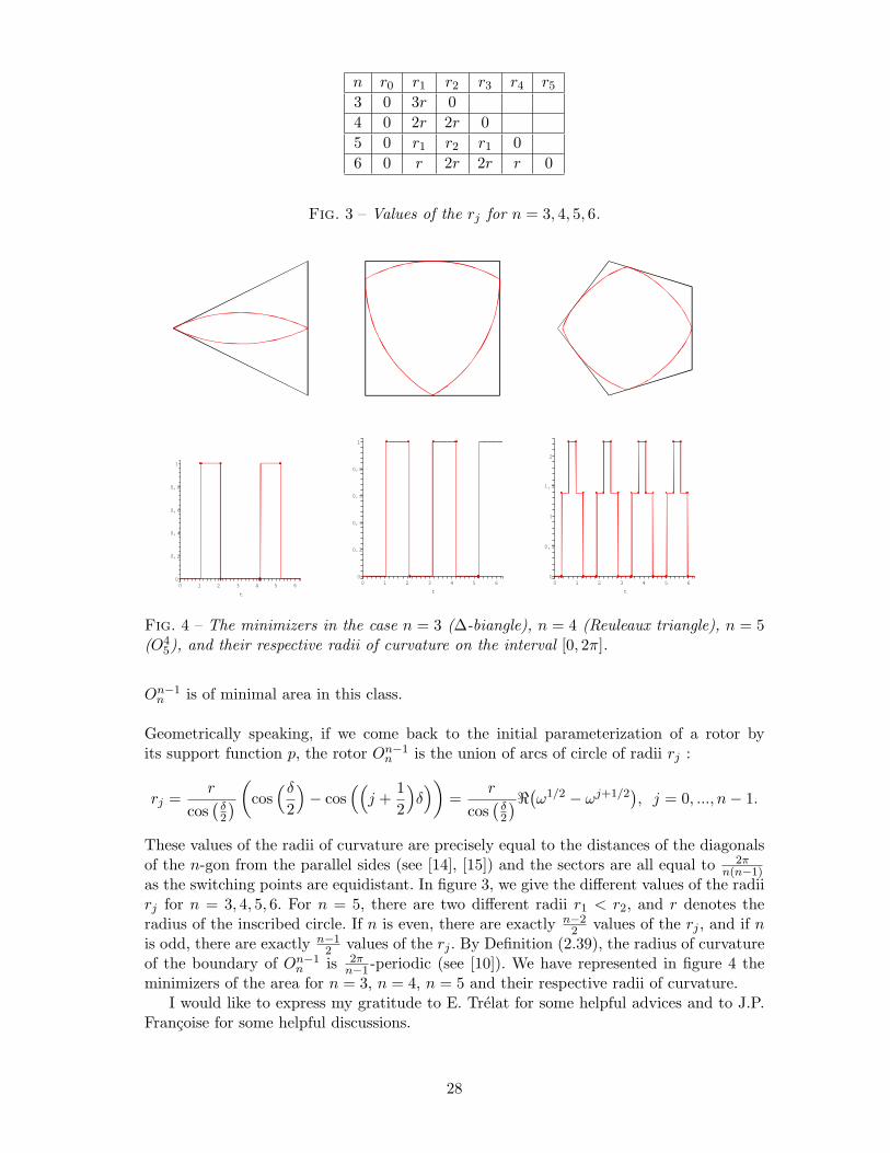
n r0 r1 r2 r3 r4 r53 0 3r 0

4 0 2r 2r 0

5 0 r1 r2 r1 0

6 0 r 2r 2r r 0

Fig. 3 – Values of the rj for n = 3, 4, 5, 6.

0

1

0,6

0,8

0,4

0

0,2

t

51 642 3

1

0,8

0,6

0,4

0,2

0

t

6543210 43210

2

1,5

1

0,5

0

t

65

Fig. 4 – The minimizers in the case n = 3 (∆-biangle), n = 4 (Reuleaux triangle), n = 5(O4

5), and their respective radii of curvature on the interval [0, 2π].

On−1n is of minimal area in this class.

Geometrically speaking, if we come back to the initial parameterization of a rotor byits support function p, the rotor On−1

n is the union of arcs of circle of radii rj :

rj =r

cos(

δ2

)

(

cos(δ

2

)

− cos((

j +1

2

)

δ)

)

=r

cos(

δ2

)ℜ(

ω1/2 − ωj+1/2)

, j = 0, ..., n− 1.

These values of the radii of curvature are precisely equal to the distances of the diagonalsof the n-gon from the parallel sides (see [14], [15]) and the sectors are all equal to 2π

n(n−1)as the switching points are equidistant. In figure 3, we give the different values of the radiirj for n = 3, 4, 5, 6. For n = 5, there are two different radii r1 < r2, and r denotes theradius of the inscribed circle. If n is even, there are exactly n−2

2 values of the rj , and if nis odd, there are exactly n−1

2 values of the rj . By Definition (2.39), the radius of curvatureof the boundary of On−1

n is 2πn−1 -periodic (see [10]). We have represented in figure 4 the

minimizers of the area for n = 3, n = 4, n = 5 and their respective radii of curvature.I would like to express my gratitude to E. Trelat for some helpful advices and to J.P.

Francoise for some helpful discussions.

28

References

[1] Andrei A. Agrachev and Yuri L. Sachkov. Control theory from the geometric viewpoint,volume 87 of Encyclopaedia of Mathematical Sciences. Springer-Verlag, Berlin, 2004., Control Theory and Optimization, II.

[2] J. A. Andrejewa and R. Klotzler. Zur analytischen Losung geometrischer Optimie-rungsaufgaben mittels Dualitat bei Steuerungsproblemen. I. Z. Angew. Math. Mech.,64(1) :35–44, 1984.

[3] J. A. Andrejewa and R. Klotzler. Zur analytischen Losung geometrischer Optimie-rungsaufgaben mittels Dualitat bei Steuerungsproblemen. II. Z. Angew. Math. Mech.,64(3) :147–153, 1984.

[4] T. Bayen, T. Lachand-Robert, and E. Oudet. Analytic parametrization of three-dimensional bodies of constant width. Arch. Ration. Mech. Anal., 186(2) :225–249,2007.

[5] Wilhelm Blaschke. Konvexe Bereiche gegebener konstanter Breite und kleinsten In-halts. Math. Ann., 76(4) :504–513, 1915.

[6] T. Bonnesen and W. Fenchel. Theory of convex bodies. BCS Associates, Moscow, ID,1987. Translated from the German and edited by L. Boron, C. Christenson and B.Smith.

[7] G. D. Chakerian and H. Groemer. Convex bodies of constant width. In Convexityand its applications, pages 49–96. Birkhauser, Basel, 1983.

[8] Bernard Dacorogna. Introduction to the calculus of variations. Imperial College Press,London, 2004. Translated from the 1992 French original.

[9] W. J. Firey. Isoperimetric ratios of Reuleaux polygons. Pacific J. Math., 10 :823–829,1960.

[10] J. Focke. Symmetrische n-Orbiformen kleinsten Inhalts. Acta Math. Acad. Sci. Hun-gar., 20 :39–68, 1969.

[11] Matsusaburo Fujiwara. Analytical proof of Blaschke’s theorem on the curve ofconstant breadth with minimum area. Proc. Tokyo Imp. Acad. Japan, 3 :300–302,1927.

[12] Matsusaburo Fujiwara and S. Kakeya. On some problems of maxima and minima forthe curve of constant breadth and the in-resolvable curve of the equilateral triangle.Tohoku Mathemaical Journal, 11 :92–110, 1917.

[13] Mostafa Ghandehari. An optimal control formulation of the Blaschke-Lebesgue theo-rem. J. Math. Anal. Appl., 200(2) :322–331, 1996.

[14] Michael Goldberg. Trammel rotors in regular polygons. Amer. Math. Monthly, 64 :71–78, 1957.

[15] Michael Goldberg. Rotors in polygons and polyhedra. Math. Comput, 14 :229–239,1960.

[16] P. M. Gruber and J. M. Wills, editors. Handbook of convex geometry. Vol. A, B.North-Holland Publishing Co., Amsterdam, 1993.

[17] Evans M. Harrell, II. A direct proof of a theorem of Blaschke and Lebesgue. J. Geom.Anal., 12(1) :81–88, 2002.

[18] Antoine Henrot. Extremum problems for eigenvalues of elliptic operators. Frontiersin Mathematics. Birkhauser Verlag, Basel, 2006.

29

[19] Ralph Howard. Convex bodies of constant width and constant brightness. Adv. Math.,204(1) :241–261, 2006.

[20] R. Klotzler. Beweis einer Vermutung uber n-Orbiformen kleinsten Inhalts. Z. Angew.Math. Mech., 55(10) :557–570, 1975.

[21] Henri Lebesgue. Sur quelques questions de minimum, relatives aux courbes orbi-formes, et sur leurs rapports avec le calcul des variations. Journal de Mathematiques(8eme serie), 4, 1921.

[22] E Meissner. Uber die Anwendung von Fourierreihen auf einige Aufgaben der Geome-trie und Kinematik. Vierteljahresschr. Naturfor. Ges. Zurich, 54 :309–329, 1909.

[23] E Meissner. Uber Punktmengen konstanter Breite. Vierteljahresschr. Naturfor. Ges.Zurich, 56 :42–50, 1911.

[24] E Meissner. Drei Gipsmodelle von Flachen konstanter Breite. Zeitschrift der Mathe-matik und Physik, 60 :92–94, 1912.

[25] L. S. Pontryagin, V. G. Boltyanskii, R. V. Gamkrelidze, and E. F. Mishchenko. Themathematical theory of optimal processes. Translated from the Russian by K. N.Trirogoff ; edited by L. W. Neustadt. Interscience Publishers John Wiley & Sons, Inc.New York-London, 1962.

[26] F Reuleaux. The kinematics of machinery : Outline of a theory of machines. Mac-millan, London, 1876.

[27] Rolf Schneider. Convex bodies : the Brunn-Minkowski theory, volume 44 of Encyclo-pedia of Mathematics and its Applications. Cambridge University Press, Cambridge,1993.

[28] Delfim F. M. Torres. Conserved quantities along the pontryagin extremals of quasi-invariant optimal control problems. Proceedings of the 10th Mediterranean Conferenceon Control and Automation, 2002.

[29] Delfim F. M. Torres. On the Noether invariance principle for constrained optimalcontrol problems. WSEAS Trans. Math., 3(3) :620–624, 2004.

[30] Emmanuel Trelat. Controle optimal. Mathematiques Concretes. [Concrete Mathema-tics]. Vuibert, Paris, 2005. Theorie & applications. [Theory and applications].

[31] Frederick A. Valentine. Convex sets. McGraw-Hill Series in Higher Mathematics.McGraw-Hill Book Co., New York, 1964.

[32] Bernulf Weissbach. Rotoren im regularen Dreieck. Publ. Math. Debrecen, 19 :21–27(1973), 1972.

[33] I. M. Yaglom and V. G. Boltyanskii. Convex Figures. Holt, Rinehart and Winston.New York.

30