Analytical models of approximations for wave functions and energydispersion in zigzag graphene nanoribbonsMahdi Moradinasab, Hamed Nematian, Mahdi Pourfath, Morteza Fathipour, and Hans Kosina Citation: J. Appl. Phys. 111, 074318 (2012); doi: 10.1063/1.3702429 View online: http://dx.doi.org/10.1063/1.3702429 View Table of Contents: http://jap.aip.org/resource/1/JAPIAU/v111/i7 Published by the American Institute of Physics. Related ArticlesEffect of in-situ oxygen on the electronic properties of graphene grown by carbon molecular beam epitaxy grown Appl. Phys. Lett. 100, 133107 (2012) Oxygen density dependent band gap of reduced graphene oxide J. Appl. Phys. 111, 054317 (2012) Electronic structures of graphane with vacancies and graphene adsorbed with fluorine atoms AIP Advances 2, 012173 (2012) Transport properties of hybrid graphene/graphane nanoribbons Appl. Phys. Lett. 100, 103109 (2012) Lateral in-plane coupling between graphene nanoribbons: A density functional study J. Appl. Phys. 111, 043714 (2012) Additional information on J. Appl. Phys.Journal Homepage: http://jap.aip.org/ Journal Information: http://jap.aip.org/about/about_the_journal Top downloads: http://jap.aip.org/features/most_downloaded Information for Authors: http://jap.aip.org/authors

Downloaded 13 Apr 2012 to 128.131.68.147. Redistribution subject to AIP license or copyright; see http://jap.aip.org/about/rights_and_permissions

Analytical models of approximations for wave functions and energydispersion in zigzag graphene nanoribbons

Mahdi Moradinasab,1,2,a) Hamed Nematian,2,3 Mahdi Pourfath,1,2 Morteza Fathipour,1

and Hans Kosina2

1School of Electrical and Computer Engineering, University of Tehran, North Kargar St., Tehran, Iran2Institute for Microelectronics, Technische Universitat Wien, Gubhausstrabe 27-29/E360,Wien A-1040, Austria3Department of Electronics, Science and Research Branch, Islamic Azad University, Tehran, Iran

(Received 25 January 2012; accepted 28 February 2012; published online 12 April 2012)

In this work, we present analytical solutions for the wave functions and energy dispersion of zigzag

graphene nanoribbons. A nearest neighbor tight-binding model is employed to describe the electronic

band structure of graphene nanoribbons. However, an exact analytical solution for the dispersion relation

and the wave functions of zigzag nanoribbons cannot be obtained. We propose two approximations of

the discrete energies, which are valid for a wide range of nanoribbon indices. Employing these models,

selection rules for optical transitions and optical properties of zigzag graphene nanoribbons are studied.VC 2012 American Institute of Physics. [http://dx.doi.org/10.1063/1.3702429]

I. INTRODUCTION

Graphene, a one-atomic-layer carbon sheet with a honey-

comb structure has received much attention over the past few

years. An extraordinarily high carrier mobility of more than

2� 105 cm2/Vs (Refs. 1–3) makes graphene a major candidate

for future electronic applications. Graphene is also regarded

as a pivotal material in the emerging field of spin electronics,

due to spin coherence even at room temperature.4,5 One of the

many interesting properties of Dirac electrons in graphene is

the drastic change of the conductivity of graphene-based

structures with the confinement of electrons. Structures that

realize this behavior are carbon nanotubes (CNTs) and gra-

phene nanoribbons (GNRs), which impose periodic and zero

boundary conditions, respectively, on the transverse electron

wave-vector. In CNT-based devices, control over the chirality

and diameter and thus of the associated electronic bandgap

remains a major technological problem. GNRs do not suffer

this problem and thus are recognized as promising building

blocks for nano-electronic devices.6 GNRs with a width of

smaller than 10 nm with ultrasmooth edges have been fabri-

cated.7 CNTs and GNRs are represented by a pair of indices

(n and m) called the chiral vector. The edges of GNRs can sig-

nificantly affect the electronic properties of the ribbon. In the

electronic band structure of GNRs with zigzag edges

(ZGNRs), a flat band, which corresponds to localized states at

the edges, appears around the Fermi level.8 However, such

states do not appear in GNRs with armchair edges (AGNRs).8

The energy band structure of AGNRs can be obtained by mak-

ing the transverse wavenumber discrete, in accordance with

the edge boundary condition, which is analogous to the case

of carbon nanotubes, where periodic boundary conditions

apply.9 An analytical model for the dispersion relation and the

wave functions of AGNRs is presented in Ref. 10. However,

because in ZGNRs, the transverse wavenumber depends not

only on the ribbon width, but also on the longitudinal

wavenumber, the energy band structure cannot be obtained

simply by slicing the bulk graphene band structure. Therefore,

exact analytical models cannot be derived for ZGNRs.9 In this

work, we present two approximations for the wavenumber of

ZGNRs, which result in simple analytical expressions for

band structure and wave functions. We show that the analyti-

cal model is valid for a wide range of GNR indices.

The organization of this paper is as the following: In

Sec. II, the electronic structure of ZGNRs is studied. The

wavenumber approximations to reach analytical models for

the dispersion relation and the wave function are derived in

Sec. III. In Sec. IV, the models are employed to obtain opti-

cal transition rules and optical properties of ZGNRs. The

two approximations used in our models and the obtained op-

tical properties are discussed in Sec. V. Finally, Sec. VI pro-

vides concluding remarks.

II. ELECTRONIC STRUCTURE

The structure of graphene consists of two types of sub-

lattices, A and B, see Fig. 1. In graphene, three r bonds hy-

bridize in an sp2 configuration, whereas the other 2pz orbital,

which is perpendicular to the graphene layer, forms p cova-

lent bonds. Each atom in an sp2-coordination has three near-

est neighbors, located acc¼ 1.42 A away. It is well known

that the electronic and optical properties of GNRs are mainly

determined by the p electrons.11. To model these p electrons,

a nearest neighbor tight-binding approximation has been

widely used.12,13 Based on this approximation, the Hamilto-

nian can be written as

H ¼ tXhp;qiðjApihBqj þ jBqihApjÞ: (1)

jApi and jBpi are atomic wave functions of the 2pz orbitals

centered at lattice sites and are labeled as Ap and Bp,

respectively, hp; qi represents pairs of nearest neighbor sites

p and q, t ¼ hApjHjBqi � �2:7 eV is the transfer integral,

and the on-site potential is assumed to be zero.a)moradinasab@iue.tuwien.ac.at.

0021-8979/2012/111(7)/074318/9/$30.00 VC 2012 American Institute of Physics111, 074318-1

JOURNAL OF APPLIED PHYSICS 111, 074318 (2012)

Downloaded 13 Apr 2012 to 128.131.68.147. Redistribution subject to AIP license or copyright; see http://jap.aip.org/about/rights_and_permissions

The total wave function of the system is given by14

jwi ¼ CAjwAi þ CBjwBi; (2)

where jwAi and jwBi are the wave functions for sublattices A

and B, respectively,

jwAi ¼1ffiffiffiffiffiffiOA

pXN

p¼1

eikxxAp /A

p jApi; jwBi ¼1ffiffiffiffiffiffiOB

pXN

p¼1

eikxxBp /B

p jBpi;

(3)

where OA=B are the normalization factors, N is the number of

atoms in the A and B sublattices in the unit-cell of the GNR,

xA=Bp are the x-positions of the pth A/B-type carbon atoms,

and /A=Bp is the amplitude of the transverse wave function of

the pth A/B-type carbon atoms.

To obtain /p, one can substitute the ansatz for the wave

functions into the Schrodinger equation. An A-type carbon

atom at some atomic site n has one B-type atom at some atomic

site N – n and two B-type neighbors at N� nþ 1 (see Fig. 1),(t f /B

N�nþ1 þ t uBN�n ¼ E uA

n ;

t uAn�1 þ t f /A

n ¼ E uBN�nþ1:

(4)

Replacing the index n with nþ 1 in the second relation of

Eq. (4), one obtains

/BN�n ¼ ð1=EÞðt uA

n þ t f /Anþ1Þ: (5)

Substituting this relation in Eq. (4), one can rewrite

Eq. (4) as

C/An ¼ /A

nþ1 þ /An�1; (6)

with

C ¼ ðE=tÞ2 � f 2 � 1

fand

f ¼ 2cosðk � a=2Þ ¼ 2cos

ffiffiffi3p

2kxacc

� �: (7)

Due to symmetry, a similar relation holds for the B-type

carbon atoms,

C/Bn ¼ /B

nþ1 þ /Bn�1: (8)

Considering the boundary condition /A0 ¼ /B

0 ¼ 0, the solu-

tion to the recursive formula is given by (see Appendix C)

/Bn ¼

CþffiffiffiffiffiffiffiffiffiffiffiffiffiffiC2 � 4p

2

!n

� C�ffiffiffiffiffiffiffiffiffiffiffiffiffiffiC2 � 4p

2

!n

ffiffiffiffiffiffiffiffiffiffiffiffiffiffiC2 � 4p /B

1 : (9)

Depending on the values of C, Eq. (7) can have three differ-

ent solutions. For jCj > 2, /Bn has a hyperbolic solution,

where the wave function is localized at the edges of the

ribbon,

/Bn ¼

2 sinh ðnhÞffiffiffiffiffiffiffiffiffiffiffiffiffiffiC2 � 4p /B

1 ; (10)

where h is given by

C ¼ 2 cosh ðhÞ: (11)

For C¼6 2, the amplitude of the wave function increases

linearly with n. This critical case appears at the transition

point from localized states to delocalized states. For jCj < 2,ffiffiffiffiffiffiffiffiffiffiffiffiffiffiC2 � 4p

is a pure imaginary number. The solution, /Bn , is

therefore given by

/Bn ¼

Cþ iffiffiffiffiffiffiffiffiffiffiffiffiffiffi4� C2p

2

!n

� C� iffiffiffiffiffiffiffiffiffiffiffiffiffiffi4� C2p

2

!n

iffiffiffiffiffiffiffiffiffiffiffiffiffiffi4� C2p /B

1 ; (12)

/Bn ¼

2 sin ðnhÞffiffiffiffiffiffiffiffiffiffiffiffiffiffi4� C2p /B

1 ¼sin ðnhÞsin ðhÞ /B

1 ; (13)

where h is the wavenumber and is given by

C ¼ 2 cos ðhÞ: (14)

Under this condition, the wave function has an oscillatory

behavior and is not localized. The prefactors CA and CB in

Eq. (2) are found to be CA ¼ 6CB (see Appendix A). To

simplify the equations, we assume /A=B1 ¼ sinðhÞ. The result-

ing normalization factors can be obtained as O ¼ N þ 1=2

(Appendix B), and the wave functions become

jwi ¼ 1ffiffiffiffiOp

XN

n¼1

eikxxAn sinðnhÞjAni6

1ffiffiffiffiOp

XN

n¼1

eikxxBn sinðnhÞjBni:

(15)

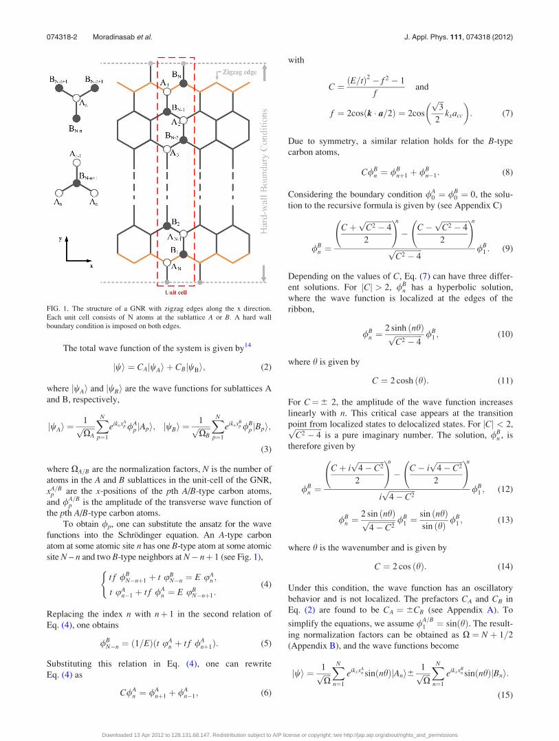
FIG. 1. The structure of a GNR with zigzag edges along the x direction.

Each unit cell consists of N atoms at the sublattice A or B. A hard wall

boundary condition is imposed on both edges.

074318-2 Moradinasab et al. J. Appl. Phys. 111, 074318 (2012)

Downloaded 13 Apr 2012 to 128.131.68.147. Redistribution subject to AIP license or copyright; see http://jap.aip.org/about/rights_and_permissions

In order to obtain the respective energy spectrum, Eq. (7)

can be written as

E ¼ 6t½Cf þ f 2 þ 1�1=2: (16)

By substituting Eq. (7) and Eq. (14) in Eq. (16), the energy

dispersion relation takes the form

E¼6t 1þ 4cos2

ffiffiffi3p

2kxacc

� �þ 4cos

ffiffiffi3p

2kxacc

� �cosðhÞ

� �1=2

:

(17)

III. WAVENUMBER APPROXIMATIONS

In the following, the relation between h and kx is

obtained. Setting n¼Nþ 1 in Eq. (4) gives

E/B0 ¼ t/A

N þ 2t cos

ffiffiffi3p

2kxacc

� �/A

Nþ1: (18)

On the other hand, the wave functions for n¼N and

n¼Nþ 1 are given by Eq. (13),

/AN ¼

sinðNhÞsinðhÞ /A

1 ; /ANþ1 ¼

sinððN þ 1ÞhÞsinðhÞ /A

1 : (19)

By imposing a hardwall boundary condition, /B0 ¼ 0, Eq. (18)

can be rewritten as

tsinðNhÞsinðhÞ /A

1 þ2tcos

ffiffiffi3p

2kxacc

� �sinððNþ1ÞhÞ

sinðhÞ /A1 ¼ 0; (20)

and we obtain the quantization condition,

sinðNhÞsinððN þ 1ÞhÞ ¼ �2 cos

ffiffiffi3p

2kxacc

� �; (21)

from Eq. (21). h can be extracted and used in the analytical

derivation of the wave functions and energy dispersion rela-

tion of ZGNRs. Figure 2 shows the variation of h as a func-

tion of kx for different subbands. As can be seen, a weak

dependency exists between h and kx. However, we assume a

constant h with respect to kx, so the right-hand side of Eq.

(21) becomes a constant. At this point, two approaches exist

to simplify Eq. (21) based on choosing kx. In general, using

all kx in the range of ½0; p=ffiffiffi3p

acc�, except kx ¼ 2p=3ffiffiffi3p

acc,

results in non-analytical solution, and curve fitting is

required to extract h. This approach is first discussed. For

kx¼ 0, Eq. (21) can be written as

sin ðNhÞsin ððN þ 1ÞhÞ ¼ �2: (22)

Using curve fitting, one finds

h ¼ Q

N þ P¼(

Q ¼ p1tþ p2

P ¼ p01tþ p02;(23)

where t is related to the subband number q (q¼ 2t) and N is

the index of ZGNR. p1, p2, p01, and p02 are fitting factors. Per-

forming a fit for the range of N 2 [6, 100],

h ¼ 3:31t� 0:5208

N þ 0:07003tþ 0:5216: (24)

Figure 3 compares h obtained from Eq. (24) with exact

numerical results.

Another approach for approximating h is selecting

kx ¼ 2p=3ffiffiffi3p

acc, which makes the right side of Eq. (21)

equal to �1,

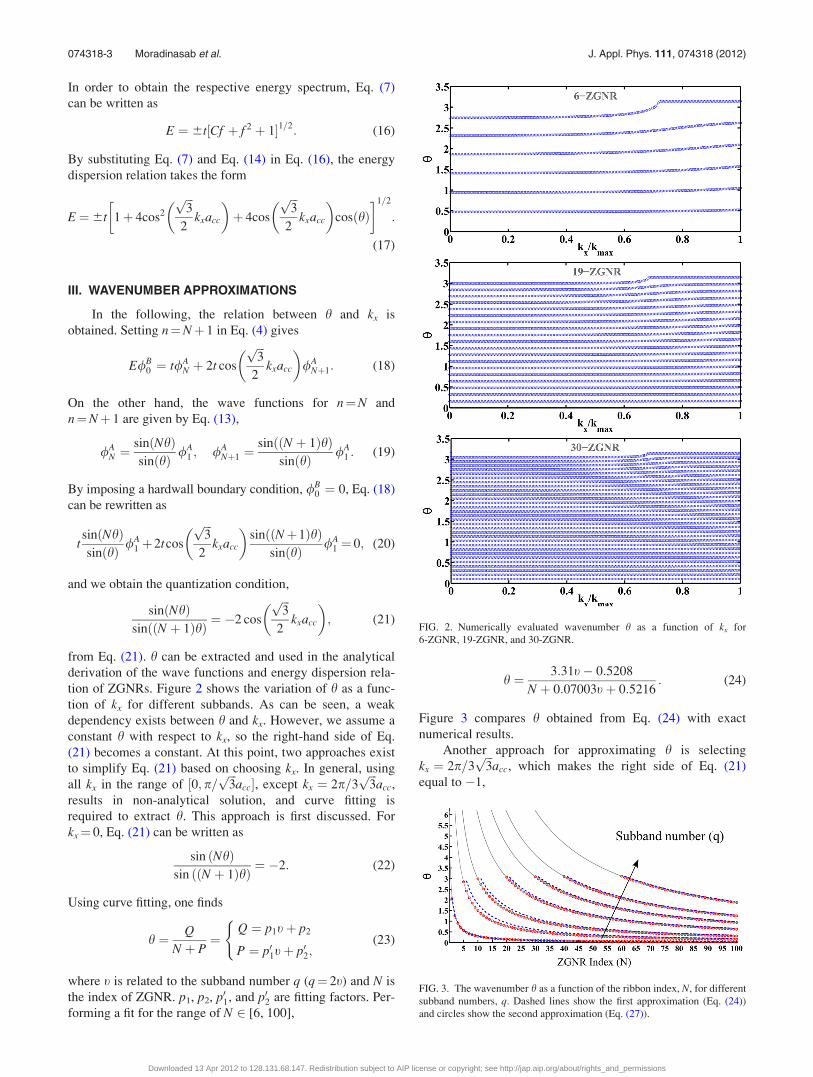
FIG. 2. Numerically evaluated wavenumber h as a function of kx for

6-ZGNR, 19-ZGNR, and 30-ZGNR.

FIG. 3. The wavenumber h as a function of the ribbon index, N, for different

subband numbers, q. Dashed lines show the first approximation (Eq. (24))

and circles show the second approximation (Eq. (27)).

074318-3 Moradinasab et al. J. Appl. Phys. 111, 074318 (2012)

Downloaded 13 Apr 2012 to 128.131.68.147. Redistribution subject to AIP license or copyright; see http://jap.aip.org/about/rights_and_permissions

sinðNhÞ þ sinððN þ 1ÞhÞ ¼ 0;

2sinðð2N þ 1Þh=2Þcosðh=2Þ ¼ 0;(25)

and has the following solution:

h ¼ tpN þ 1=2

: (26)

By representing t in terms of subband index q, h is obtained

as a function of q and N,

h ¼ qp2N þ 1

: (27)

Figure 3 compares the discussed approximations with exact

numerical results. The value of h for Eq. (27) shows a good

agreement with that obtained from numerical calculations.

The approximation is valid for a wide range of ZGNR indi-

ces. Using the analytical expression for h, analytical wave

functions and energy dispersion are evaluated from Eq. (15)

and Eq. (17). The results for a 6-ZGNR and a 19-ZGNR are

shown in Fig. 4 and Fig. 5, respectively.

IV. OPTICAL MATRIX ELEMENTS AND TRANSITIONRULES

Optical transition rules can be obtained from the optical

matrix elements. The interband optical matrix element deter-

mines the probability for a transition from a state jmi to a final

state jni and is given by ðe=m0ÞhnjA � pjmi,15 where e is

the elementary charge, m0 is the electron mass, A ¼ Ae is the

vector potential, e is a unit vector parallel to A, and p is the

linear momentum operator. The vector potential can be sepa-

rated from the expectation value, assuming the wave vector of

the electromagnetic field is negligible compared to the elec-

tronic wave vector (dipole approximation). As a result, optical

matrix elements can be achieved by evaluating momentum

matrix elements, hnje � pjmi. In this work, the electromagnetic

field is assumed to be polarized along the x direction.

pn;m ¼ hnjpxjmi: (28)

Knowing the wave function of atomic orbitals,16 the matrix

elements of the momentum operator can be calculated from

Eq. (28). However, in most of the tight-binding models, the

atomic orbitals are unknown, a difficulty which is usually

circumvented by the gradient approximation.17 By using the

operator relation p ¼ ðim0=�hÞ [H, r], Eq. (28) can be rewrit-

ten as pn;m ¼ ðim0=�hÞhnjHx� xHjmi. In this approximation,

intra-atomic transitions are ignored. However, as we employ

a single orbital model to describe the electronic band struc-

ture of ZGNRs, intra-atomic transitions are intrinsically

neglected. Therefore, the momentum matrix elements can be

approximated as18

pn;m ¼ ðxm � xnÞim0

�hhnjHjmi: (29)

With the wave functions derived in Sec. II, evaluation of

transition rules from Eq. (29) is possible. Using the wave

functions from Eq. (15) in Eq. (29), and considering only

nearest neighbors, one can obtain (see Appendix D)

Ph;h0 ¼2ffiffiffi3p

m0acct

�hð2N þ 1Þ sin

ffiffiffi3p

2kacc

� �X2N

n¼1

hsinðnh0Þsinðð2N � nþ 1ÞhÞ

� sinðnhÞsinðð2N � nþ 1Þh0Þi: (30)

The upper limit of summation 2N is due to degenerate points

of valance and conduction bands at kx ¼ 62p=3ffiffiffi3p

acc. The

subband indices are included in h and h0 [see Eq. (27)].

The summation over sine functions in Eq. (30) determines

the transition rules. By some trigonometric identities, one

can rewrite this summation as follows:

Ph;h0 ¼�2

ffiffiffi3p

m0acct

�hð2Nþ 1Þ sin

ffiffiffi3p

2kacc

� �

cos�ð2Nþ 1Þðhþ h0Þ=2

�sin�2Nðh� h0Þ=2

�sin�ðh� h0Þ=2

�"

�cos�ð2Nþ 1Þðh� h0Þ=2

�sin�2Nðhþ h0Þ=2

�sin�ðhþ h0Þ=2

�#:

(31)

Using the analytical approximation of h in Eq. (27) for the

cosine terms in Eq. (31) gives

cos�ð2N þ 1Þðh6h0Þ=2

�¼ cos ðq6q0Þ p

2

: (32)

If q¼ 2rþ 1 and q0 ¼ 2r0 or q¼ 2r and q0 ¼ 2r0 þ 1, where

r and r0 are non-zero integers, q 6 q0 ¼ 2r00 þ 1, both terms in

the bracket of Eq. (31) will be zero. In the case of q¼ 2r and

q0 ¼ 2r0 or q¼ 2rþ 1 and q0 ¼ 2r0 þ 1, the terms in the

bracket will be non-zero. Therefore, the transitions between

valence and conduction subbands only with the same parity

(odd to odd and even to even) are allowed,

Ph;h0 ¼ Pq;q0

¼0; if q¼ odd ðevenÞ and q0 ¼ even ðoddÞ;6¼ 0; if q¼ odd ðevenÞ and q0 ¼ odd ðevenÞ:

�(33)

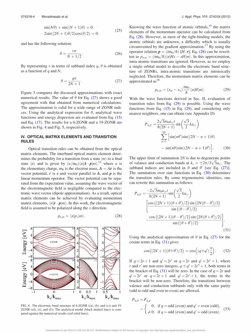
FIG. 4. The electronic band structure of 6-ZGNR ((a), (b), and (c)) and 19-

ZGNR ((d), (e), and (f)). The analytical model (black dashed lines) is com-

pared against the numerical results (red solid lines).

074318-4 Moradinasab et al. J. Appl. Phys. 111, 074318 (2012)

Downloaded 13 Apr 2012 to 128.131.68.147. Redistribution subject to AIP license or copyright; see http://jap.aip.org/about/rights_and_permissions

V. RESULTS AND DISCUSSION

In this section, the energy dispersion relation and the wave

functions for the approximated discrete wavenumbers h are

evaluated and compared against exact numerical calculations.

Equation (27) is employed to give the wave functions

and energy dispersions from Eq. (15) and Eq. (17), respec-

tively. Based on the structure depicted in Fig. 1, the width of

a zigzag nanoribbon is given by

W ¼ 3N

2þ 1

� �acc; (34)

where acc¼ 1.42 A is the carbon-carbon bond length in gra-

phene. For ZGNRs with a width below 50 nm, indices in the

range 6 to 235 have to be considered. In this range of indices,

the wave functions and the energy dispersion have been eval-

uated. It should be noted that structures wider than 50 nm are

also evaluated, and the results show excellent agreement

with those obtained from numerical simulation. Figure 6

shows several wave functions for 125-ZGNR evaluated from

two approximations proposed. As can be seen, the wave

functions obtained by Eq. (27) are matched very well with

the numerical calculations. The dispersion relation of some

subbands for 125-ZGNR is shown in Fig. 7. Similar to the

wave functions, the dispersion relations obtained by h from

Eq. (27) show well agreement with the numerical results.

An important conclusion that one can draw from these

results is that the analytical approximation of h presented in

Eq. (27) is more accurate than the solution obtained by using

a curve fitted h (see Fig. 6 and Fig. 7). Also, the accuracy of

the analytical method increases as the ZGNR index increases

(see the energy dispersions for 6-ZGNR and 19-ZGNR in

Fig. 4 and 125-ZGNR in Fig. 7). As can be seen in Fig. 2,

this increase in accuracy is due to the fact that h is relatively

independent of changes in the wave-vector (kx) for large val-

ues of N. In order to investigate the applicability of the

FIG. 5. The wave functions of 6-ZGNR and 19-ZGNR. Red(blue) symbols denote the wave functions in sublattice B(A). The analytical model (squares) is

compared against the numerical results (circles).

074318-5 Moradinasab et al. J. Appl. Phys. 111, 074318 (2012)

Downloaded 13 Apr 2012 to 128.131.68.147. Redistribution subject to AIP license or copyright; see http://jap.aip.org/about/rights_and_permissions

proposed models, the optical matrix elements are derived

analytically based on our models in Sec. IV. To evaluate the

transition rules, we can also investigate the symmetry of the

transition matrix element in Eq. (28). If the symmetry of this

element spans the totally symmetric representation of the

point group to which the unit cell belongs, then its value is

not zero and the transition is allowed. Otherwise, the transi-

tion is forbidden. Assuming a uniform potential profile

across the ribbon’s width, the subbands’ wave functions are

either symmetric or antisymmetric along the y direction,

h�yjwc=ti ¼ 6hyjwc=ti: (35)

Considering the wave functions for 6-ZGNR and 19-ZGNR

(Fig. 5), subbands corresponding to odd indices are symmet-

ric, while those corresponding to even indices are

antisymmetric.

Therefore, the momentum matrix elements are non-zero

for transitions from the symmetric (antisymmetric) to the

symmetric (antisymmetric) wave functions. This transition

rule results in transitions from subbands with odd (even) to

odd (even) indices in ZGNRs,19 which confirms the result

obtained from our analytical derivation of the wave functions

and momentum matrix elements.

The imaginary part of the dielectric function is used to

investigate the optical properties of a material.15 If the inci-

dent light is assumed to be polarized along the transport

direction (x-axis), the imaginary part of the dielectric func-

tion in the linear response regime is given by15

eiðxÞ ¼1

4pe0

2pe

mx

� �2

�X

kx

jpc;tj2dðEcðkxÞ � EtðkxÞ � �hxÞ;

(36)

where �hx is the energy of the incident photons and pc,t are

the momentum matrix elements for optical transitions (Ph;h0

in our study). To demonstrate the applicability of our mod-

els, the imaginary part of the dielectric function ei is calcu-

lated numerically for 6-ZGNR and 19-ZGNR [see Fig. 8(a)

and Fig. 8(b)]. Peaks in ei(x) indicate absorptions of photons

with energy �hx. From the electronic band structure in Fig.

8(c), it can be found that the peaks in ei(x) are related to

transitions from n¼ 6 to n¼ 8 (A) and n¼ 6 to n¼ 10 (C).

FIG. 7. The electronic band structure of 125-

ZGNR. The analytical model (red symbols) and

the curve fitted (blue symbols) are compared

with the numerical results (black symbols).

FIG. 6. The wave functions of 125-ZGNR. Red(blue) symbols denote the

wave functions at the sublattice B(A). The analytical model (squares) and

curve-fitted model (diamonds) are compared against the numerical results

(circles) for different subbands.

FIG. 8. Dielectric function of (a) 6-ZGNR and (b) 19-ZGNR. The peaks are

related to electronic band structure of (c) 6-ZGNR and (d) 19-ZGNR.

074318-6 Moradinasab et al. J. Appl. Phys. 111, 074318 (2012)

Downloaded 13 Apr 2012 to 128.131.68.147. Redistribution subject to AIP license or copyright; see http://jap.aip.org/about/rights_and_permissions

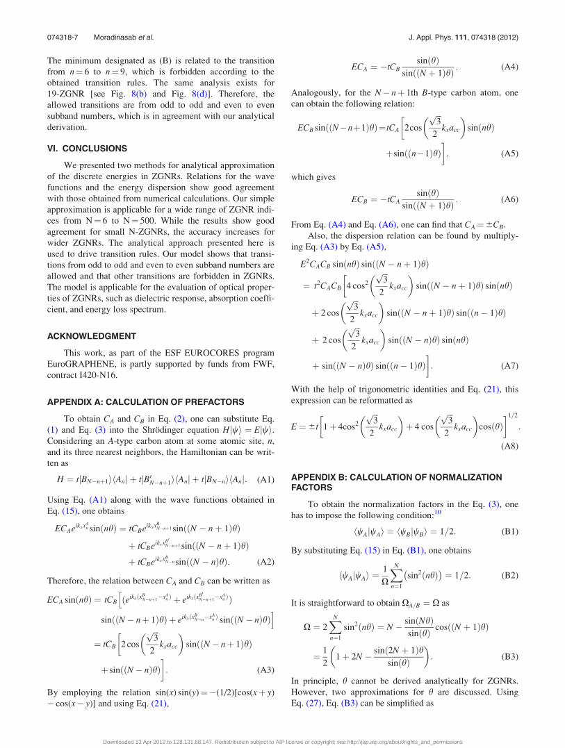
The minimum designated as (B) is related to the transition

from n¼ 6 to n¼ 9, which is forbidden according to the

obtained transition rules. The same analysis exists for

19-ZGNR [see Fig. 8(b) and Fig. 8(d)]. Therefore, the

allowed transitions are from odd to odd and even to even

subband numbers, which is in agreement with our analytical

derivation.

VI. CONCLUSIONS

We presented two methods for analytical approximation

of the discrete energies in ZGNRs. Relations for the wave

functions and the energy dispersion show good agreement

with those obtained from numerical calculations. Our simple

approximation is applicable for a wide range of ZGNR indi-

ces from N¼ 6 to N¼ 500. While the results show good

agreement for small N-ZGNRs, the accuracy increases for

wider ZGNRs. The analytical approach presented here is

used to drive transition rules. Our model shows that transi-

tions from odd to odd and even to even subband numbers are

allowed and that other transitions are forbidden in ZGNRs.

The model is applicable for the evaluation of optical proper-

ties of ZGNRs, such as dielectric response, absorption coeffi-

cient, and energy loss spectrum.

ACKNOWLEDGMENT

This work, as part of the ESF EUROCORES program

EuroGRAPHENE, is partly supported by funds from FWF,

contract I420-N16.

APPENDIX A: CALCULATION OF PREFACTORS

To obtain CA and CB in Eq. (2), one can substitute Eq.

(1) and Eq. (3) into the Shrodinger equation Hjwi ¼ Ejwi.Considering an A-type carbon atom at some atomic site, n,

and its three nearest neighbors, the Hamiltonian can be writ-

ten as

H ¼ tjBN�nþ1ihAnj þ tjB0N�nþ1ihAnj þ tjBN�nihAnj: (A1)

Using Eq. (A1) along with the wave functions obtained in

Eq. (15), one obtains

ECAeikxxAn sinðnhÞ ¼ tCBeikxxB

N�nþ1 sinððN � nþ 1ÞhÞ

þ tCBeikxxB0N�nþ1 sinððN � nþ 1ÞhÞ

þ tCBeikxxBN�n sinððN � nÞhÞ: (A2)

Therefore, the relation between CA and CB can be written as

ECA sinðnhÞ ¼ tCB ðeikxðxBN�nþ1

�xAn Þ þ eikxðxB0

N�nþ1�xA

n ÞÞh

sinððN� nþ 1ÞhÞ þ eikxðxBN�n�xA

n Þ sinððN� nÞhÞi

¼ tCB

�2 cos

ffiffiffi3p

2kxacc

� �sinððN� nþ 1ÞhÞ

þ sinððN� nÞhÞ�: (A3)

By employing the relation sin(x) sin(y)¼�(1/2)[cos(xþ y)

� cos(x� y)] and using Eq. (21),

ECA ¼ �tCBsinðhÞ

sinððN þ 1ÞhÞ : (A4)

Analogously, for the N� nþ 1th B-type carbon atom, one

can obtain the following relation:

ECB sinððN�nþ1ÞhÞ¼tCA

�2cos

ffiffiffi3p

2kxacc

� �sinðnhÞ

þsinððn�1ÞhÞ�; (A5)

which gives

ECB ¼ �tCAsinðhÞ

sinððN þ 1ÞhÞ : (A6)

From Eq. (A4) and Eq. (A6), one can find that CA¼6CB.

Also, the dispersion relation can be found by multiply-

ing Eq. (A3) by Eq. (A5),

E2CACB sinðnhÞ sinððN � nþ 1ÞhÞ

¼ t2CACB 4 cos2

ffiffiffi3p

2kxacc

� �sinððN � nþ 1ÞhÞ sinðnhÞ

�

þ 2 cos

ffiffiffi3p

2kxacc

� �sinððN � nþ 1ÞhÞ sinððn� 1ÞhÞ

þ 2 cos

ffiffiffi3p

2kxacc

� �sinððN � nÞhÞ sinðnhÞ

þ sinððN � nÞhÞ sinððn� 1ÞhÞ�: (A7)

With the help of trigonometric identities and Eq. (21), this

expression can be reformatted as

E¼6t 1þ 4cos2

ffiffiffi3p

2kxacc

� �þ 4 cos

ffiffiffi3p

2kxacc

� �cosðhÞ

� �1=2

:

(A8)

APPENDIX B: CALCULATION OF NORMALIZATIONFACTORS

To obtain the normalization factors in the Eq. (3), one

has to impose the following condition:10

hwAjwAi ¼ hwBjwBi ¼ 1=2: (B1)

By substituting Eq. (15) in Eq. (B1), one obtains

hwAjwAi ¼1

O

XN

n¼1

sin2ðnhÞ� �

¼ 1=2: (B2)

It is straightforward to obtain OA=B ¼ O as

O ¼ 2XN

n¼1

sin2ðnhÞ ¼ N � sinðNhÞsinðhÞ cosððN þ 1ÞhÞ

¼ 1

21þ 2N � sinð2N þ 1Þh

sinðhÞ

� �: (B3)

In principle, h cannot be derived analytically for ZGNRs.

However, two approximations for h are discussed. Using

Eq. (27), Eq. (B3) can be simplified as

074318-7 Moradinasab et al. J. Appl. Phys. 111, 074318 (2012)

Downloaded 13 Apr 2012 to 128.131.68.147. Redistribution subject to AIP license or copyright; see http://jap.aip.org/about/rights_and_permissions

O ¼ N þ 1=2: (B4)

APPENDIX C: RECURSIVE FORMULA SOLUTION

To solve the recursive formula,

/nþ1 � C/n þ /n�1 ¼ 0; (C1)

one can consider the ansatz /n¼ tn and follow the similar

equation,

t2 � Ctþ 1 ¼ 0: (C2)

This equation is the generating polynomial of the recursive

formula Eq. (C1). The roots of Eq. (C2) are

t1;2 ¼ðC6

ffiffiffiffiffiffiffiffiffiffiffiffiffiffiffiffiC2 � 4Þ

p2

: (C3)

The general solution of the difference equation is

/n ¼ atn1 þ btn2: (C4)

Since t1 is a root of the equation, the other root, t2, can be

written as t2 ¼ t�11 .

By substituting those two roots in Eq. (C4), one obtains

/n ¼ atn1 þ bt�n1 : (C5)

Imposing the initial condition, /0¼ 0, results in

aþ b ¼ 0; a ¼ �b; (C6)

and from the Eq. (C5),

/n ¼ aðtn1 � t�n

1 Þ: (C7)

As a result,

a ¼ /1ffiffiffiffiffiffiffiffiffiffiffiffiffiffiC2 � 4p ; b ¼ � /1ffiffiffiffiffiffiffiffiffiffiffiffiffiffi

C2 � 4p : (C8)

By substituting Eq. (C3) and Eq. (C8) in Eq. (C7), one obtains

/n ¼/1ffiffiffiffiffiffiffiffiffiffiffiffiffiffi

C2 � 4p Cþ

ffiffiffiffiffiffiffiffiffiffiffiffiffiffiC2 � 4p

2

!n

� /1ffiffiffiffiffiffiffiffiffiffiffiffiffiffiC2 � 4p C�

ffiffiffiffiffiffiffiffiffiffiffiffiffiffiC2 � 4p

2

!n

: (C9)

Eq. (C9) can be rewritten as

/n ¼Cþ

ffiffiffiffiffiffiffiffiC2�4p

2

n� C�

ffiffiffiffiffiffiffiffiC2�4p

2

n

ffiffiffiffiffiffiffiffiffiffiffiffiffiffiC2 � 4p /1: (C10)

APPENDIX D: OPTICAL MATRIX ELEMENTS

Using Eq. (15) and Eq. (29), the matrix elements

ph;h0 ðkxÞ � hþ; h; kxjpxj�; h0; kxi for an interband transition

from a valence band state j�; h; kxi to a conduction band

state jþ; h0; kxi are obtained as

Ph;h0 ¼ ðxh0 � xhÞim0

�hhhjHjh0i; (D1)

Ph;h0 ¼im0

�hO

XN

n¼1

XN

m¼1

eikðxBm�xA

n ÞsinðnhÞsinðmh0ÞhAnjHjBmiðxBm � xA

n Þ � eikðxAm�xB

n Þsinðnh0ÞsinðmhÞhBnjHjAmiðxAm � xB

n Þh i

: (D2)

Considering only the nearest neighbors, each atom with some

index, n, has two neighbors with index N� nþ 1 and one

neighbor with index N� n (see Fig. 1). Therefore, the index,

m, has only three values, with hAnjHjBmi ¼ t. So we have

Ph;h0 ¼im0

�hO

� �iffiffiffi3p

acct

2

� �XN

n¼1

ðeiffiffi3p

kxa=2 � e�iffiffi3p

kxa=2Þ sinðnhÞ sinððN � nþ 1Þh0Þh

�ðe�iffiffi3p

kxa=2 � eiffiffi3p

kxa=2Þ sinðnh0Þ sinððN � nþ 1ÞhÞi: (D3)

After some algebra and replacing O from Eq. (B4), the optical matrix elements are

Ph;h0 ¼�2

ffiffiffi3p

m0acct

�hð2N þ 1Þ sin

ffiffiffi3p

2kacc

� �XN

n¼1

hsinðnhÞsinððN � nþ 1Þh0Þ � sinðnh0ÞsinððN � nþ 1ÞhÞ

i: (D4)

1X. Du, I. Skachko, A. Barker, and E. Andrei, Nat. Nanotechnol. 3, 491

(2008).2K. Bolotin, K. Sikesb, Z. Jianga, M. Klimac, G. Fudenberga, J. Honec, P.

Kima, and H. Stormera, Solid-State Commun. 146, 351 (2008).3J.-H. Chen, C. Jang, S. Xiao, M. Ishighami, and M. Fuhrer, Nat. Nanotech-

nol. 3, 206 (2008).

4N. Tombros, C. Jozsa, M. Popinciuc, H. Jonkman, and B. van Wees, Na-

ture (London) 448, 571 (2008).5S. Cho, Y.-F. Chen, and M. Fuhrer, Appl. Phys. Lett. 91, 123105

(2007).6M. Freitag, Nat. Nanotechnol. 3, 455 (2008).7X. Li, L. Zhang, S. Lee, and H. Dai, Science 319, 1229 (2008).

074318-8 Moradinasab et al. J. Appl. Phys. 111, 074318 (2012)

Downloaded 13 Apr 2012 to 128.131.68.147. Redistribution subject to AIP license or copyright; see http://jap.aip.org/about/rights_and_permissions

8K. Nakada, M. Fujita, G. Dresselhaus, and M. S. Dresselhaus, Phys. Rev.

B 54, 17954 (1996).9K. Wakabayashi, K. I. Sasaki, T. Nakanishi, and T. Enoki, Sci. Technol.

Adv. Mater. 11, 054504 (2010).10H. Zheng, Z. Wang, T. Luo, Q. Shi, and J. Chen, Phys. Rev. B 75, 165414

(2007).11R. Saito, G. Dresselhaus, and M. Dresselhaus, Physical Properties of Car-

bon Nanotubes (Imperial College Press, London, 1998).12S. Reich, J. Maultzsch, C. Thomsen, and P. Ordejon, Phys. Rev. B 66,

035412 (2002).

13Y. Hancock, A. Uppstu, K. Saloriutta, A. Harju, and M. J. Puska, Phys.

Rev. B 81, 245402 (2010).14S. V. Goupalov, Phys. Rev. B 72, 195403 (2005).15P. T. Yu and M. Cardona, Fundamentals of Semiconductors: Physics and

Materials Properties (Springer, Berlin, 2001).16A. K. Gupta, O. E. Alon, and N. Moiseyev, Phys. Rev. B 68, 205101

(2003).17G. Dresselhaus and M. S. Dresselhaus, Phys. Rev. 160, 649 (1967).18T. G. Pedersen, Phys. Rev. B 67, 113106 (2003).19H. Hsu and L. E. Reichl, Phys. Rev. B 76, 045418 (2007).

074318-9 Moradinasab et al. J. Appl. Phys. 111, 074318 (2012)

Downloaded 13 Apr 2012 to 128.131.68.147. Redistribution subject to AIP license or copyright; see http://jap.aip.org/about/rights_and_permissions