Analytical Modeling of Beyond Visual Range Air Combat

Analytical Modeling of Beyond Visual Range AirCombat

Darin Corman, [email protected] (A project report writtenunder the guidance of Prof. Raj Jain) Download

Abstract

The paper reviews fundamental beyond-visual-range air-combat analytical models and enhances thesemodels. In particular, the fundamental models reviewed are sequential missile exchanges. A one-versus-onemodel is developed to handle the case when both sides are destroyed in a single exchange. The paper thandevelops an analytical model that takes into account engagement geometry, detection range, aircraft speed,missile speed, and missile seeker type for a single missile exchange. This type of model can be used to predictthe order of missile exchanges.

Keywords: Air Combat, Beyond Visual Range, Analytical Modeling

Table of Contents

1. Introduction2. Fundamental Analytical Models 2.1 Undefended Target - One-Sided Engagements 2.2 One Versus One Sequential Engagements 2.3 Many Versus Many One-Sided Engagements3. Extentions To Fundamental Analytical Models 3.1 One Versus One Sequential Engagement - Mutual Kills 3.2 Including Engagement Geometry, Detection, Speed, And Different Weapon Technologies4. Conclusion5. Acronyms6. References

1. Introduction

There is an extensive history of applying mathematics to military science. During World War II the professionoperations research was created to use mathematics to address military problems. During the same timeperiod, warfare was changing rapidly due to new technology such as aircraft. A new branch of the UnitedStates Military was founded, the Air Force, to best exploit this new domain of warfare. Since its inception, theAir Force has relied on science and mathematics to determine investments in technology and form itsdoctrine. The quintessential model of combat was developed by Lanchester while contemplating the impactaircraft would have on warfare (1). During the cold war simple analytical models were developed and used tounderstand air-to-air combat in the jet-age. The Rand Corporation played a key role in the development ofthese models.

Analytical Modeling of Beyond Visual Range Air Combat

1 of 13

Today, simulation is the main tool used to study complex military problems. Performance analysis of variousmilitary systems and systems-of-systems is often the subject. There are many reasons for the predominance ofsimulation in the study of the performance of military systems. The reasons are not unique to the study ofmilitary systems, for example Dr Jain's book on computer systems performance analysis outlines the strengthsof computer simulation (2). Among them are moderate fidelity, moderate abstraction, and the ability to studysystems that do not yet exist. All of these reasons make it more saleable to decision makers. Nevertheless,simulation can be a time intensive and still requires verification from other methods such as measurement,analytical models, or expert opinion. Analytical models, while lacking detail, are simple and fast. They areuseful as screening tools and understanding more complex simulations. They can also be used in largecomputer simulations when fast run times are necessary or when a simulation requires modeling aphenomenon but it is not the subject of the study. In order to be accepted by decision makers, theassumptions that are made in analytical models must not impair the purpose of the analysis.

Historic analytical models to study air combat for beyond-visual-range (BVR) missile exchanges, whilehaving there place, do not take into account factors important to current-day aircraft. At the very least auseful model should include the geometry of the engagement, detections, speeds, and types of missiles used.The purpose of this paper is two-fold. The first objective is to survey several analytical models of air-to-airBVR missile exchanges. The second objective is to expand on these models to create a useful model toanalyze current and future aircraft performance.

2. Fundamental Analytical Models

2.1 Undefended Target - One-Sided Engagements

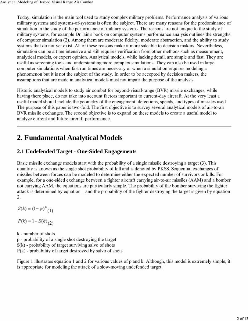
Basic missile exchange models start with the probability of a single missile destroying a target (3). Thisquantity is known as the single shot probability of kill and is denoted by PKSS. Sequential exchanges ofmissiles between forces can be modeled to determine either the expected number of survivors or kills. Forexample, for a one-sided exchange between a fighter aircraft carrying air-to-air missiles (AAM) and a bombernot carrying AAM, the equations are particularly simple. The probability of the bomber surviving the fighterattack is determined by equation 1 and the probability of the fighter destroying the target is given by equation2.

(1)

(2)

k - number of shotsp - probability of a single shot destroying the targetS(k) - probability of target surviving salvo of shotsP(k) - probability of target destroyed by salvo of shots

Figure 1 illustrates equation 1 and 2 for various values of p and k. Although, this model is extremely simple, itis appropriate for modeling the attack of a slow-moving undefended target.


2 of 13

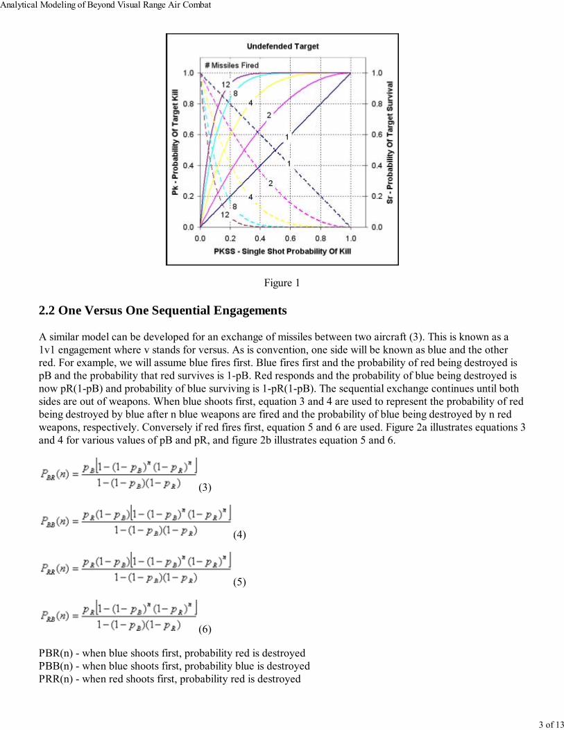
Figure 1

2.2 One Versus One Sequential Engagements

A similar model can be developed for an exchange of missiles between two aircraft (3). This is known as a1v1 engagement where v stands for versus. As is convention, one side will be known as blue and the otherred. For example, we will assume blue fires first. Blue fires first and the probability of red being destroyed ispB and the probability that red survives is 1-pB. Red responds and the probability of blue being destroyed isnow pR(1-pB) and probability of blue surviving is 1-pR(1-pB). The sequential exchange continues until bothsides are out of weapons. When blue shoots first, equation 3 and 4 are used to represent the probability of redbeing destroyed by blue after n blue weapons are fired and the probability of blue being destroyed by n redweapons, respectively. Conversely if red fires first, equation 5 and 6 are used. Figure 2a illustrates equations 3and 4 for various values of pB and pR, and figure 2b illustrates equation 5 and 6.

(3)

(4)

(5)

(6)

PBR(n) - when blue shoots first, probability red is destroyedPBB(n) - when blue shoots first, probability blue is destroyedPRR(n) - when red shoots first, probability red is destroyed


3 of 13

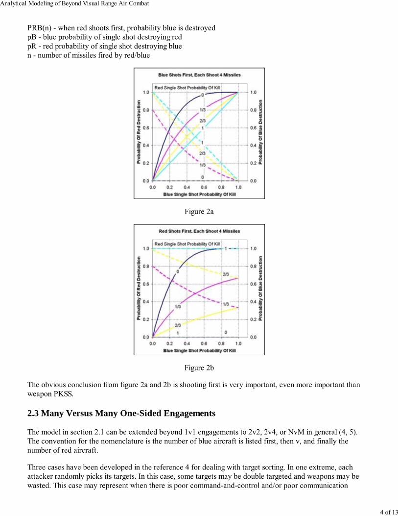
PRB(n) - when red shoots first, probability blue is destroyedpB - blue probability of single shot destroying redpR - red probability of single shot destroying bluen - number of missiles fired by red/blue

Figure 2a

Figure 2b

The obvious conclusion from figure 2a and 2b is shooting first is very important, even more important thanweapon PKSS.

2.3 Many Versus Many One-Sided Engagements

The model in section 2.1 can be extended beyond 1v1 engagements to 2v2, 2v4, or NvM in general (4, 5).The convention for the nomenclature is the number of blue aircraft is listed first, then v, and finally thenumber of red aircraft.

Three cases have been developed in the reference 4 for dealing with target sorting. In one extreme, eachattacker randomly picks its targets. In this case, some targets may be double targeted and weapons may bewasted. This case may represent when there is poor command-and-control and/or poor communication


4 of 13

between the individual attackers. The other extreme is perfect target sorting where all attackers uniformlydistribute weapons over the targets. This case represents when the attackers and/or their controllers havegood communication and the ability to effectively sort targets. The third case is an extension of the secondwhere the attackers and/or their controllers have the ability to make a good kill assessment allowing them tofocus new salvos only on surviving targets.

This paper will focus on the simple extension of the 1v1 engagement to an NvN engagement. It is important todemonstrate that 1v1 results can be extended to many-on-many, but the details can be worked out in latter. Inthis situation N = M, and each attacker is assigned a single target. In addition the attacker expends all itsmissiles on its assigned target. Equations 7-10 can be used to determine the average number of survivors afterthe engagement is complete.

(7)

(8)

(9)

(10)

J - number of weapons per attackerM - number of attackersN - total number of weponsT - number of targetsp J - probability of kill for J shotsp - probability of a single shot destroying the targetSr - average survivability of each targetE S - expected number of surviving targets

Since M = T, equations 7-10 can be simplified to equation 11.

(11)

3. Extentions To Fundamental Analytical Models

3.1 One Versus One Sequential Engagement - Mutual Kills

Although the chance of both sides getting destroyed simultaneously may seem remote, with missiles that areactively guided in the terminal phase it can occur. This type of missile only needs to be guided by the attackerto within a certain range of the target, and then the attacker may disengage from the fight. This is advantagecompared to the less sophisticated semi-active guided missile that must be guided all the way to the target (4).The author was not able to find the derivation of a 1v1 sequential engagement in which both sides' shotsarrive simultaneously resulting in a mutual kill. Therefore equations are derived for this situation. The missilesin this case no longer arrive sequentially, but each side's volley arrives simultaneously. With each volley thereare four potential outcomes: both sides are destroyed, red is destroyed and blue survives, red survives andblue is destroyed, or both sides survive. For example, equation 12 is the probability red is destroyed in thefirst exchange. It is the sum of the probability both sides are destroyed, and red is destroyed and bluesurvives.


5 of 13

(12)

Similarly, equation 13 represents the probability red is destroyed in the second volley. It is the probability thatred and blue survived the first volley multiplied by the two cases where red is destroyed.

(13)

The natural result of this procedure is a general equation for n shots. Equation 14 and 15 represent theprobability of destruction after n shots for red and blue, respectively.

(14)

(15)

A careful reader will note the resulting equation 12 is the same as equation 3. Similarly equation 13 is thesame as equation 6.

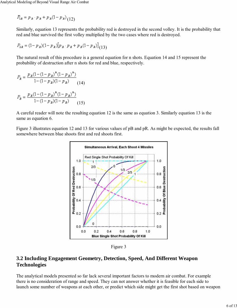
Figure 3 illustrates equation 12 and 13 for various values of pB and pR. As might be expected, the results fallsomewhere between blue shoots first and red shoots first.

Figure 3

3.2 Including Engagement Geometry, Detection, Speed, And Different WeaponTechnologies

The analytical models presented so far lack several important factors to modern air combat. For examplethere is no consideration of range and speed. They can not answer whether it is feasible for each side tolaunch some number of weapons at each other, or predict which side might get the first shot based on weapon


6 of 13

system characteristics. To answer these deficiencies it is necessary to introduce ranges and speeds. Reference5 develops an analytical model that includes these important factors. The model that follows, builds on thatdeveloped in reference 5 for our purposes.

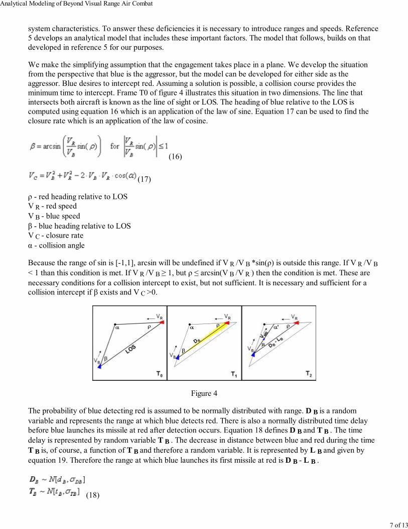
We make the simplifying assumption that the engagement takes place in a plane. We develop the situationfrom the perspective that blue is the aggressor, but the model can be developed for either side as theaggressor. Blue desires to intercept red. Assuming a solution is possible, a collision course provides theminimum time to intercept. Frame T0 of figure 4 illustrates this situation in two dimensions. The line thatintersects both aircraft is known as the line of sight or LOS. The heading of blue relative to the LOS iscomputed using equation 16 which is an application of the law of sine. Equation 17 can be used to find theclosure rate which is an application of the law of cosine.

(16)

(17)

ρ - red heading relative to LOSV R - red speedV B - blue speedβ - blue heading relative to LOSV C - closure rateα - collision angle

Because the range of sin is [-1,1], arcsin will be undefined if V R /V B *sin(ρ) is outside this range. If V R /V B< 1 than this condition is met. If V R /V B ≥ 1, but ρ ≤ arcsin(V B /V R ) then the condition is met. These arenecessary conditions for a collision intercept to exist, but not sufficient. It is necessary and sufficient for acollision intercept if β exists and V C >0.

Figure 4

The probability of blue detecting red is assumed to be normally distributed with range. D B is a randomvariable and represents the range at which blue detects red. There is also a normally distributed time delaybefore blue launches its missile at red after detection occurs. Equation 18 defines D B and T B . The timedelay is represented by random variable T B . The decrease in distance between blue and red during the timeT B is, of course, a function of T B and therefore a random variable. It is represented by L B and given byequation 19. Therefore the range at which blue launches its first missile at red is D B - L B .

(18)


7 of 13

(19)

A desired characteristic of the model is the blue aircraft must detect the red aircraft before launching itsmissile. The normal distribution, assumed for simplicity, can violate this condition. Care must be taken tochoose a t B and σ TB such that the probability of launching before detection is very small i.e. t B should be 3σTB away from 0.

The line the blue missile flies is different than the blue aircraft because the blue missile is traveling at adifferent speed. For simplicity it is assumed the speed at which the missile travels is the summation of theaircraft speed and a base missile speed. The line the missile follows is determined by equations 20 - 22.

(20)

(21)

(22)

V MB - blue missile speed without including speed imparted by launching aircraftμ B - blue missile heading relative to line of sightα MB - blue missile collision angle with red aircraftV CMB - closure rate of blue missile and red aircraftR MB - distance blue missile flies to get to red aircraft

The distance separating blue and red once the blue missile destroys red is D B - L B - M B . Equation 23 isused to calculate M B . The quantity R MB / V CMB is the time of flight (TOF) of the missile. Equation 24 isfound by substituting for M B in D B - L B - M B

(23)

(24)

Radar seekers are most common for BVR missiles. There are two types of radar seekers used: semi-activeradar (SAR) and active radar (AR). For air combat, AR seekers have been used on newer missiles. SARguided missiles must be supported until impact with the target. AR guided missiles only have to be supporteduntil the missile is within a certain range of the target (4). The advantages of this can be seen in theapplication of the above developed model.

As in reference 5, the probability of blue destroying red before red reaches launch range can be computed.This computation is for a SAR guided missile. This computation and comparison is a good way to validate theanalytical model. The condition that must be met for blue to destroy red before red reaches launch range is


8 of 13

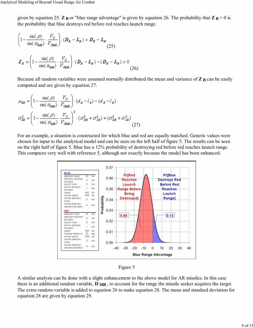
given by equation 25. Z B or "blue range advantage" is given by equation 26. The probability that Z B > 0 isthe probability that blue destroys red before red reaches launch range.

(25)

(26)

Because all random variables were assumed normally distributed the mean and variance of Z B can be easilycomputed and are given by equation 27.

(27)

For an example, a situation is constructed for which blue and red are equally matched. Generic values werechosen for input to the analytical model and can be seen on the left half of figure 5. The results can be seenon the right half of figure 5. Blue has a 12% probability of destroying red before red reaches launch range.This compares very well with reference 5, although not exactly because the model has been enhanced.

Figure 5

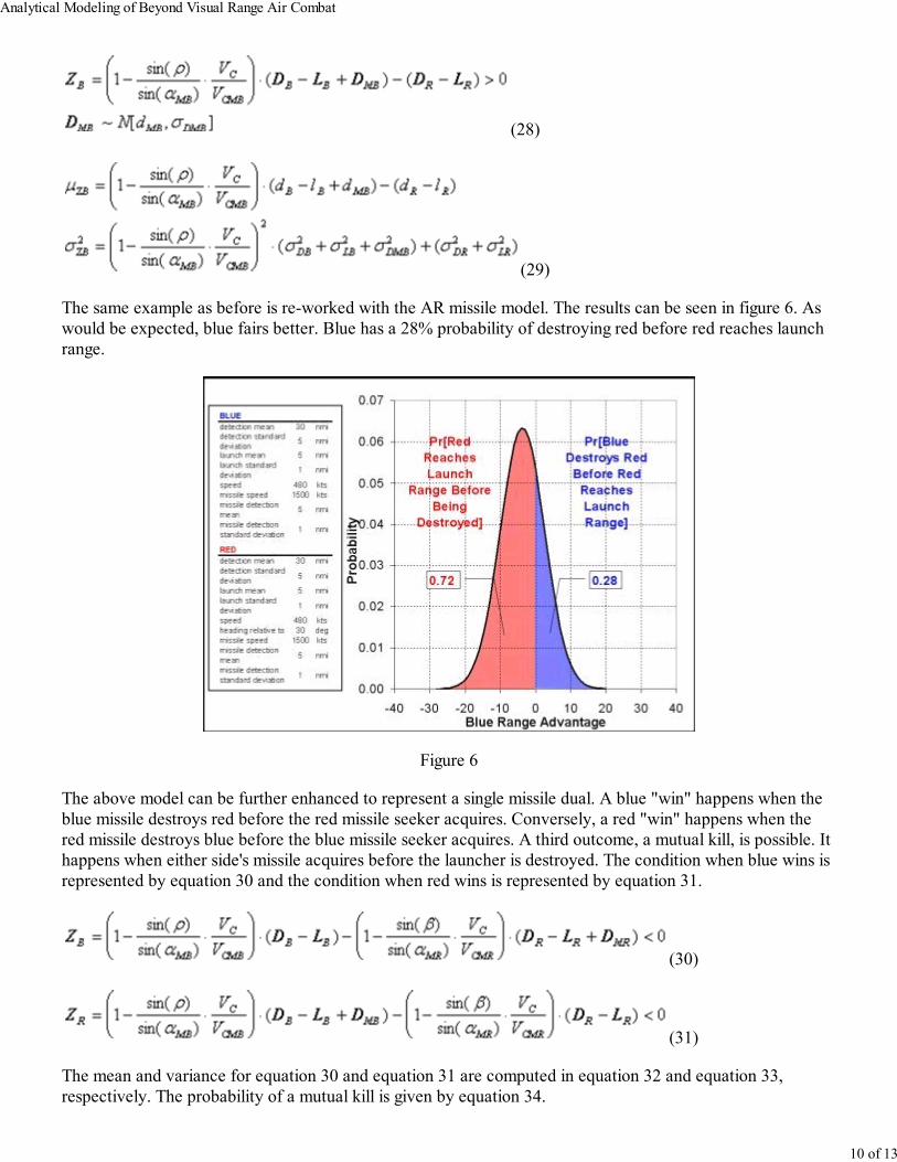
A similar analysis can be done with a slight enhancement to the above model for AR missiles. In this casethere is an additional random variable, D MB , to account for the range the missile seeker acquires the target.The extra random variable is added to equation 26 to make equation 28. The mean and standard deviation forequation 28 are given by equation 29.


9 of 13

(28)

(29)

The same example as before is re-worked with the AR missile model. The results can be seen in figure 6. Aswould be expected, blue fairs better. Blue has a 28% probability of destroying red before red reaches launchrange.

Figure 6

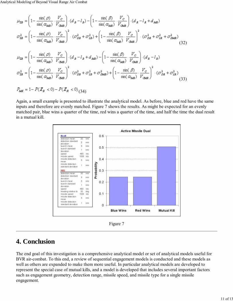
The above model can be further enhanced to represent a single missile dual. A blue "win" happens when theblue missile destroys red before the red missile seeker acquires. Conversely, a red "win" happens when thered missile destroys blue before the blue missile seeker acquires. A third outcome, a mutual kill, is possible. Ithappens when either side's missile acquires before the launcher is destroyed. The condition when blue wins isrepresented by equation 30 and the condition when red wins is represented by equation 31.

(30)

(31)

The mean and variance for equation 30 and equation 31 are computed in equation 32 and equation 33,respectively. The probability of a mutual kill is given by equation 34.


10 of 13

(32)

(33)

(34)

Again, a small example is presented to illustrate the analytical model. As before, blue and red have the sameinputs and therefore are evenly matched. Figure 7 shows the results. As might be expected for an evenlymatched pair, blue wins a quarter of the time, red wins a quarter of the time, and half the time the dual resultin a mutual kill.

Figure 7

4. Conclusion

The end goal of this investigation is a comprehensive analytical model or set of analytical models useful forBVR air-combat. To this end, a review of sequential engagement models is conducted and these models aswell as others are expanded to make them more useful. In particular analytical models are developed torepresent the special case of mutual kills, and a model is developed that includes several important factorssuch as engagement geometry, detection range, missile speed, and missile type for a single missileengagement.


11 of 13

Sequential models are fundamental because more complex models usually result in a PKSS exchange. If thisis the case, regardless of the complexity of the model, the results can be reproduced if the exchange order isknown e.g. a tree diagram can be used to determine probabilities of survival, etc (4). Unfortunately, theexchange is rarely "textbook" back and forth. Models that take into account engagement geometries andspeed are necessary to predict the exchange order and how many weapons are exchanged per time period.

The utility of a "toolbox" of analytical models would be the ability to quickly conduct performance analysis.In particular, a design of experiment (DOE) using an analytical model could help understand the relativeimportance of factors such as detection range, speed, and number of weapons carried. The understandinggained from relatively simple analytical models can help verify more complex simulations.

Unfortunately, the small progress made in this report falls well short of a comprehensive analytical modelingtoolbox. In particular a many-on-many sequential engagement model is missing. The limited amount of workdone on developing a many-on-many sequential engagement model reveals some of the pitfalls of analyticalmodeling. For example, unsatisfactory assumptions are often necessary to obtain a closed-form solution.Nevertheless, the special cases where closed-form solutions exist can be used to validate more generalspreadsheet models.

8. Acronyms

AAM - air-to-air missileAR - active radarBVR - beyond visual rangeDOE - design of experimentsLOAL - lock-on after launchLOBL - lock-on before launchLOS - line of sightPKSS - probability of kill single shotSAR - semi-active radarTOF - time of flight

9. References

F. W. Lanchester, Aircraft In Warfare: The Dawn Of The Fourth Arm, 1916.1.Raj Jain, The Art Of Computer Systems Performance Analysis: Techniques for Experimental DesignMeasurement, Simulation, and Modeling, 1991.

2.

J.S. Przemieniecki, Mathematical Methods In Defense Analyses, 3rd Ed, AIAA Education Series, 2000.3.Robert E. Ball, The Fundamentals Of Aircraft Combat, Survivability Analysis And Design, 2nd Ed,AIAA Education Series, 2003.

4.

Lester E. Dubins and George W. Morgenthaler, "Inclusion of Detection in Probability of SurvivalModels," Operations Research, November 1961, 782-801.

5.

Daniel H. Wagner, W. Charles Mylander, and Thomas J. Sanders, Naval Operations Analysis 3rd Ed,Navel Institute Publishing, 1999.

6.

Last modified on November 24, 2008This and other papers on latest advances in performance analysis are available on line athttp://www.cse.wustl.edu/~jain/cse567-08/index.html


12 of 13

Back to Raj Jain's Home Page


13 of 13

Documents

Analytical Modeling of Beyond Visual Range Air Combat