Abstract— Roball is a spherical robot designed to be a

platform to study child-robot interaction in open settings. It has

a spherical shell and uses motors attached along its rolling axis

plus an actuated counterweight for steering. It is designed to be

inexpensive and to generate a wide variety of movement. To

evaluate its locomotion capabilities in relation to the size and

weight of its components, we have derived analytical models

describing its longitudinal and lateral motion. Simulation

results are presented using MATLAB/Simulink and

SimMechanics, and validated using a real robot.

I. INTRODUCTION

spherical rolling robot is a mobile platform that moves

by using a mechanism that either change the center of

gravity or generate a force to make the robot roll on its outer

shell. Spherical rolling robots can be categorized into six

categories:

• A single driving wheel placed at the bottom inside a

sphere, attached to axis supporting a controlling box, a

spring and a balance wheel [1][2].

• A spherical wheel with an arch-shaped body outside the

sphere, similar to a mono-cycle robot [3].

• A hollow sphere with a small car [4] resting on the

bottom of the sphere. The concept is similar to having a

gerbil run inside a spherical plastic ball.

• A sphere with two side rotors, mutually perpendicular,

plus one rotor attached to the bottom of the sphere [5].

The change in angular velocities of these internal rotors

turning on themselves makes the robot move.

• A sphere with four inertial wheels [6][7] or masses that

move [8] over four axes in a tethrahedral structure.

• A sphere with motors attached to the side of the sphere

at the position of the rolling axis. A rotational mass [9]

or an actuated counterweight [10] [11] can be used to

steer the robot.

Surveys of ball-shaped and spherical robots are presented

in [2][4][12].

This work was supported in part by the Canada Research Chair (CRC),

the Natural Sciences and Engineering Research Council of Canada

(NSERC) and the Canadian Foundation for Innovation (CFI).

Jean-François Laplante and Patrice Masson are with the Department of

Mechanical Engineering of the Université de Sherbrooke, Québec

CANADA J1K 2R1 (e-mail: {Jean-Francois.Laplante,

Patrice.Masson}@USherbrooke.ca).

F. Michaud holds the Canada Research Chair in Mobile Robotics and

Intelligent Autonomous Systems. He is with the Department of Electrical

Engineering and Computer Engineering of the Université de Sherbrooke,

Québec CANADA J1K 2R1 (phone: 819-821-8000 x 62107; fax: 819 821-

7937; e-mail: Francois.Michaud@USherbrooke.ca).

Fig. 1. First (left) and second (right) prototypes of Roball.

Our robot, named Roball [10][11][13][14], fits in the last

category. Roball is made of three rigid bodies: its spherical

outer shell, its internal structure holding the different internal

components of the robot (motors, microcontroller and

circuits), and its counterweight. We built two prototypes of

Roball: Roball-1 is made of a plastic sphere (bought in a pet

store) attached at the middle, and Roball-2 is designed to be

manufactured by thermoforming and was fabricated using

Rapid Prototyping in ABS (acrylonitrile-butadiene-styrene

copolymers) plastic. Shown in Fig. 1, both are about 6

inches in diameter. Propulsion motors are located on the side

of the internal structure, perpendicular (on the horizontal

plane) to the front heading of the robot and attached to the

extremities of the spherical shell. They move the center of

gravity of the robot forward or backward, for longitudinal

motion of the robot. The speed of the motors is regulated

according to longitudinal inclination of the internal structure,

keeping the center of gravity of the robot close to the

ground. Lateral motion is achieved using the battery as the

counterweight, mounted on a servo-motor. This allows the

robot to tilt on one side or the other as the shell rolls.

Since cost is an issue in designing a toy robot for child-

robot interaction [13], we used inexpensive sensors such as

tilt sensors (first prototype using two propulsion motors –

resolution approximately 30° over 160°) or custom-designed

inclinometers using small pendulums, wheel encoders and

photodetectors (second prototype using one propulsion

motor – resolution 10° over 360°) to provide control

measurement for velocity control of the robot’s motors. Such

increased range is required with Roball-2 because its

steering mechanism allows the robot to flip over from one

side to the other, over 250°, as shown in Fig. 2. Note that

with one of its side being flat (the other is the robot’s face),

Roball-2 can lie with its face facing upward, to facilitate

interaction with people.

Even though the six categories of spherical rolling robots

have implemented prototypes, not all have detailed

Analytical Longitudinal and Lateral Models of a Spherical Rolling

Robot

Jean-François Laplante, Patrice Masson and François Michaud

A

mathematical models of the robot’s motion capabilities. In

relation to other types of spherical rolling robots, only [3]

and [4] present models for longitudinal motion that can show

similarities with Roball, but following different locomotion

principles. For a spherical robot like Roball, to our

knowledge, no kinematic and dynamic models of

longitudinal or lateral motions have yet been developed. For

our work, advanced models would not be necessary to derive

a controller for the robot because of the low-precision

sensors used onboard. Simple models are desired to evaluate

the influence of the robot’s weight and diameter on its

motion.

Fig. 2. Roball-2 moving from one side to another, by moving its internal

counterweight. The middle picture illustrates how Roball-2 can lie face up.

In this paper, we present models that describe

mathematically the robot’s longitudinal and lateral motion

capabilities on flat surfaces, first described using

MATLAB/Simulink in Section II, and then validated using

SimMechanics and experimentally using Roball-2 as

reported in Section III.

II. MOTION MODELS

A. Longitudinal Motion

Let us start with a simplified model, only considering no-

slip longitudinal motion on flat surfaces. Fig. 3 illustrates the

simplified model with a side view of the robot. It represents

the spherical outer shell with its center of mass CMS and a

pendulum (composed of a massless link and a point mass at

its end) with center of mass CMQ and the axis attached at the

center of the sphere.

Fig. 3. Simplified model for longitudinal motion, side view of the robot.

Dynamic models can be derived for the pendulum and the

sphere using Newton-Euler method, summing the forces and

summing the moments. Fig. 4 illustrates the forces and

moments on each of the two rigid bodies. The sum of forces

on the pendulum expressed in relation to X and Y reference

frame is given by (1), with RX and RY the reacting forces at

the point of contact of the axis, rQ being the length of the

pendulum’s shaft, g is the gravitational acceleration, and ˙ ̇ x S

being the longitudinal acceleration of the sphere.

RX

RY

+ mQ

0

g

= mQ

˙ ̇ QrQ cos Q˙ Q

2rQ sin Q + ˙ ̇ x S˙ ̇ QrQ sin Q + ˙ Q

2rQ cos Q + 0

(1)

The sum of moments on the pendulum is presented by (2),

with C being the torque applied at the center of the sphere

and JQ the moment of inertia of the pendulum about an axis

perpendicular to the X-Y plane.

C mQrQgsin Q = JQ ˙ ̇ Q (2)

Fig. 4. Forces and moments for the pendulum (left) and the sphere (right).

The sum of forces and the sum of moments for the sphere

are given by (3) and (4) respectively, with f representing the

contact force, N the normal force with the ground, rS being

the radius of the sphere, JS the inertia of the sphere about an

axis perpendicular to the X-Y plane, and ˙ ̇ S the angular

acceleration of the sphere.

RX

RY

+ mS

0

g

+

f

N

= mS

˙ ̇ x S0

(3)

C + f rS = JS ˙ ̇ S (4)

The longitudinal acceleration of the sphere can be

expressed in terms of the angular acceleration of the sphere

according to (5).

˙ ̇ x S = ˙ ̇ SrS (5)

Fig. 5.

Q (left) and ˙ S (right) in relation to time using the non-linear

longitudinal model, with mS = 0.448 kg, rS = 0.0889 m, JS = 2.35x10-3 kg

m2, mQ = 0.5 kg, rQ = 0.0317 m, JQ = 5.025x10-4 kg m2.

Fig. 5 illustrates Q

and ˙ S with respect to time with a

step excitation of C = 0.01 Nm, using (1) to (5) is generated

in a MATLAB/Simulink simulation. The results indicate that

the system oscillates around a mean value of Q = 0.7 rad,

and such oscillations have an impact on the speed of the

sphere ˙ S .

In order to simulate Roball’s behavior, a model of its

propulsion actuator, i.e., a DC motor, must be derived.

Equations (6) and (7) present this model, with L the motor’s

inductance, R its resistance, kE the back electromotive force

(back-emf) constant, kM the torque constant constant, Z the

gear ratio, and i and e the current and applied voltage

respectively.

L˙ i + Ri + kE Z ˙ S ˙ Q( ) = e (6)

C = kM Zi (7)

Considering only the forces in the X axis and using these

seven equations, three non-linear equations are derived

expressing the longitudinal dynamic model of the robot.

Equation (8) is obtained by isolating RX in (1) and (3),

isolating f using (4) replacing ˙ ̇ x S by (5) and replacing C by

(7). Equation (9) is derived from replacing (7) in (2).

Equation (10) is derived directly from (6).

mQ (rQ ˙ ̇ Q cos Q rQ ˙ Q2 sin Q rS ˙ ̇ S ) +

kM Zi JS ˙ ̇ SrS

mSrS ˙ ̇ S = 0 (8)

JQ ˙ ̇ Q + mQrQgsin Q kM Zi = 0 (9)

L˙ i + Ri + kE Z ˙ S ˙ Q( ) e = 0 (10)

Using (8), (9) and (10), a linear model is expressed with

state variables of the form uBxAx +=& , with u equals to e,

is given by (11) and (12). The model is linearized at Q = 0

and ˙ Q = 0 .

˙ S˙ ̇ S˙ Q˙ ̇ Q˙ i

=

0 1 0 0 0

0 0mQ

2 rQ2rS g

G 0mQ rQ rS kM +kM ZJQ

G

0 0 0 1 0

0 0mQ rQ g

JQ0 kM Z

JQ

0 kE ZL 0 kE Z

LR

L

S

˙ S

Q

˙ Qi

+ e

0

0

0

01L

(11)

G = JQ mQrS2 + mSrS

2 + JS( ) (12)

Using the linear longitudinal model, we can demonstrate

that the system is controllable by state feedback [14] in order

to remove the oscillations shown in Fig. 5. However, with

Roball-2, to minimize the cost, we only have onboard

inclinometers installed on the robot, a small microcontroller

and no velocity sensors measuring the sphere’s speed of

rotation. It is therefore impossible to implement a complete

state-based control approach with Roball-2. The control

strategy is thus to assign a constant speed setpoint for the

sphere, and to use the angle Q

of Roball-2’s internal

structure measured by the inclinometer as the error signal.

At constant velocity and without considering friction,

Q 0 .

Fig. 6 illustrates the pole-zero map of the open-loop

transfer function of the system, derived using the linear

model given by (11). It shows an angular frequency of 3.85

rad/s and a damping of 0.089. For a unit step input, the gain

of the steady state response would be -0.8525.

Fig. 6. Pole-zero map (left) and unit step input (right) of the linear

longitudinal model, with kE = 3.3517x10-3 V/rad, kM = 2.130x10-3 N m/A.

Fig. 7. Effect of KBF on the pole-zero map.

In a closed-loop configuration, a proportional controller

with gain KBF can stabilize Q

around the desired position.

Fig. 7 shows the effect of KBF on the pole-zero map. As KBF

increases, the conjugated pole is moving away from the

imaginary axis while the real pole is moving closer, and

eventually the system becomes over-damped. KBF=0.126 is

the smallest gain for which the system remains over-damped

and stable. This results for a system with a rise time of 0.62

sec, no overshoot, a natural frequency of 4.2 rad/s and a

damping of 1, as shown in Fig. 8.

Fig. 8. Pole-zero map (left) and unit step input (right) of the linear

longitudinal model with KBF =0.126.

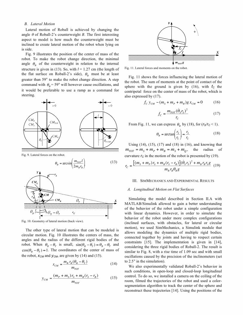
B. Lateral Motion

Lateral motion of Roball is achieved by changing the

angle of Roball-2’s counterweight B. The first interesting

aspect to model is how much the counterweight must be

inclined to create lateral motion of the robot when lying on

is side.

Fig. 9 illustrates the position of the center of mass of the

robot. To make the robot change direction, the minimal

angle B of the counterweight in relation to the internal

structure is given in (13). So, with l = 1.27 cm (the length of

the flat surface on Roball-2’s side), B must be at least

greater than 59° to make the robot change direction. A step

command with B = 59° will however cause oscillations, and

it would be preferable to use a ramp as a command for

steering.

Fig. 9. Lateral forces on the robot.

B = arcsin

mTOT l

2mBrB

(13)

Fig. 10. Geometry of lateral motion (back view).

The other type of lateral motion that can be modeled is

circular motion. Fig. 10 illustrates the centers of mass, the

angles and the radius of the different rigid bodies of the

robot. When B T is small, sin( B T ) B T and

cos( B T ) 1. The coordinates of the center of mass of

the robot, xCM and yCM, are given by (14) and (15).

xCM =mB rB ( B T )

mTOT

(14)

yCM =(mP + mS ) rS + mB (rS rB )

mTOT

(15)

Fig. 11. Lateral forces and moments on the robot.

Fig. 11 shows the forces influencing the lateral motion of

the robot. The sum of moments at the point of contact of the

sphere with the ground is given by (16), with fC the

centripetal force on the center of mass of the robot, which is

also expressed by (17).

fC yCM (mS + mP + mB )g xCM = 0 (16)

fC =mTOT ( ˙ SrS )2

rC (17)

From Fig. 11, we can express B by (18), for (rS/rC < 1).

B = arctan

rSrC

rSrC

(18)

Using (14), (15), (17) and (18) in (16), and knowing that

mTOT = mS + mP + mB = mS + mQ , the radius of

curvature rC in the motion of the robot is presented by (19).

rC =(mS + mP ) rS + mB (rS rB )[ ]( ˙ S rS )2 + mB rBrSg

mB rB Bg (19)

III. SIMMECHANICS AND EXPERIMENTAL RESULTS

A. Longitudinal Motion on Flat Surfaces

Simulating the model described in Section II.A with

MATLAB/Simulink allowed to gain a better understanding

of the behavior of the robot under a simple configuration

with linear dynamics. However, in order to simulate the

behavior of the robot under more complex configurations

(inclined surfaces, with obstacles, for lateral or circular

motion), we used SimMechanics, a Simulink module that

allows modeling the dynamics of multiple rigid bodies,

connected together by joints and having to respect certain

constraints [15]. The implementation is given in [14],

considering the three rigid bodies of Roball-2. The result is

similar to Fig. 8, with a rise time of 1.09 sec and with small

oscillations caused by the precision of the inclinometers (set

to 2.5° in the simulation).

We also experimentally validated Roball-2’s behavior in

such conditions, in open-loop and closed-loop longitudinal

control. To do so, we installed a camera on the ceiling of the

room, filmed the trajectories of the robot and used a color-

segmentation algorithm to track the center of the sphere and

reconstruct these trajectories [14]. Using the positions of the

robot as a function of time, the velocity of the sphere can be

derived. Fig. 12 shows all of the results obtained with a

velocity setpoint of 4 rad/s with Roball-2 and with

SimMechanics. Compared to the simulation, more

oscillations occur with the real robot. This is caused by the

fact that the resolution of the inclinometer used on the robot

is 10°. To avoid inadequate behavior, inclinometer data

between ±10° are set to 0. This limitation causes oscillations

but, despite that, the closed-loop control allows reducing by

60% the oscillations in the angular speed of the robot,

compared to the open-loop configuration.

Fig. 12. Unit step input of Roball in open and closed loops with KBF =0.126

using SimMechanics.

B. Lateral Motion

Fig. 13 shows results obtained using this model for

different rotational velocities ˙ S . The round dots represent

results obtained using SimMechanics for ( ˙ S , B ) = (2 rad/s,

9°) and for ( ˙ S , B ) = (4 rad/s, 24°). MATLAB/Simulink

simulation results are shown for 2 rad/s, 3 rad/s and 4 rad/s.

Fig. 13. Radius of curvature in relation to the angle of the counterweight,

for different rotational velocities of the sphere.

Fig. 14. Circular trajectories made by Roball at ( ˙ S ,

B) = (3 rad/s, 45°).

Using the ceiling camera setup, we validated some of

these results using Roball-2 at ˙ S =3 rad/s and B set to 15°,

30° and 45°. Fig. 14 illustrates one trial. It is worth noticing

that the center of the circular trajectories moves as the robot

turn. This is caused by low-resolution readings of the

inclinometer (used in a PI controller of the angle of the

counterweight), unbalanced masses in the robot and small

inclination of the floor. Considering each complete circle

made by the robot and averaging the radius of curvature,

results in Fig. 13 shows good similarities between the

mathematical model and the trajectories of the real robot.

Finally, changing the setpoint for B over time allows

creating interesting trajectories like a spiral or an 8-figure, as

shown from simulation in Fig. 15. Such trajectories were

reproduced with Roball-2, but with less precision because of

the limitations of its onboard sensors. However, such sensors

are sufficient for generating interesting trajectories that will

keep children engaged in interacting with the robot.

Fig. 15. Spiral (top) and 8-figure (bottom) trajectories with ˙ S = 3 rad/s over

a 2m 2m area. The assigned setpoints for B

over time are shown on the

left, and on the right top views of the trajectories made by the robot are

shown.

IV. CONCLUSION

Manufacturing custom spherical shelves is expensive,

and being capable of anticipating the influence of the robotic

components’ weights and size before fabricating the robot

would be quite helpful. Spherical robots have complex

dynamics, and being able to simulate their behavior would

be quite valuable in the design process.

In this paper, we have presented non-linear and linear

models of longitudinal and lateral motions of a spherical

rolling robot that applies a torque at the rolling axis and can

control the position of a counterweight for steering.

Experimental trials done using Roball-2 confirm the validity

of the models, considering the resolution of its onboard

sensors.

Future work involves the design of new prototypes of

Roball of different sizes and weights, making the shell as

robust and light as possible, and to use these prototypes to

study infant-robot interaction [13]. As of now, Roball’s

prototypes were designed without any use of models to set

its size, weight, radius of the flat surface of its side, etc. The

models described in this paper will be useful in helping

evaluate the motion capabilities of different versions of

Roball before going into fabrication.

ACKNOWLEDGMENT

The authors want to acknowledge the contributions of

Serge Caron and Dominic Létourneau in building Roball’s

second prototype. Special thanks to Michel Lauria for his

helpful comments in reviewing this paper.

REFERENCES

[1] S. Halme, T. Schönberg, and Y. Wang, “Motion control of a spherical

mobile robot,” in Proc. Int. Workshop on Advanced Motion Control, Japan, 1996.

[2] K. Husay, Instrumentation of a Spherical Mobile Robot, Master’s

Thesis, Department of Engineering Cybernetics, Trondheim

06.08.2003, 2003.

[3] A. Koshiyama and K. Yamafuji, “Design and control of an all-

direction steering type mobile robot,” The International Journal of Robotics Research, vol. 12, no. 5, pp. 411-419, 1993.

[4] A. Bicchi, A. Balluchi, D. Prattichizzo, A. Gorelli, “Introducing the

Sphericle: An experimental testbed for research and teaching in non-

holonomy,” in Proc. IEEE Int. Conf. on Robotics and Automation,

1997.

[5] S. Bhattacharya and S. K. Agrawal, “Spherical rolling robot: A design

and motion planning studies,” IEEE Transactions on Robotics and Automation, vol. 16, no. 6, pp. 835-839, 2000.

[6] R. Mukherjee and M. Minor, “A simple motion planner for a spherical

mobile robot,”, in Proc. IEEE/ASME Int. Conf. on Advanced Intelligent Mechatronics, pp. 896-877, 1999.

[7] R. Mukherjee and T. Das, “Feedback stabilization of a spherical

mobile robot,” Proc. IEEE/RSJ Int. Conf. on Intelligent Robots and Systems, pp. 2154-2162, 2002.

[8] A. Javadi and P. Mojabi, “Introducing August: A novel strategy for an

omnidirectional spherical rolling robot,” in Proc. IEEE Int. Conf. on Robotics and Automation, pp. 3527-3533, 2002.

[9] B. Chemel, E. Mustcheler, and H. Schempf, “Cyclops: Miniature

robotic reconnaissance system,” in Proc. IEEE Int. Conf. on Robotics and Automation, 1999.

[10] F. Michaud and S. Caron, “Roball, the rolling robot,” Autonomous Robots, vol. 2, no. 12, pp. 211-222, 2002.

[11] F. Michaud and S. Caron, “Roball – the rolling robot (Patent style),”

U.S. Patent #6,227,933, May 8, 2001.

[12] J. Suomela and T. Ylikorpi, “Ball-shaped robots: An historical

overview and recent development at TKK,” Field and Service Robots, STAR 25, pp. 343-354, 2006.

[13] J.-F. Laplante, F. Michaud, H. Larouche, A. Duquette, S. Caron, D.

Létourneau, P. Masson, “Autonomous spherical mobile robot to study

child development,” IEEE Trans. on Systems, Man, and Cybernetics, Part A, vol. 35, no. 4, pp. 471-480, 2005.

[14] J.-F. Laplante, Étude de la dynamique d’un robot sphérique et de son effet sur l’attention et la mobilité de jeunes enfants, Masters thesis,

Department of Mechanical Engineering, Université de Sherbrooke,

Sherbrooke, Québec Canada, 2004.

[15] G. D. Woods, “Simulating mechanical systems in Simulink with

SimMechanics,” The MathWorks inc., 2003.