Embed Size (px)
Citation preview
Universität der Bundeswehr München
Fakultät für Elektrotechnik und Informationstechnik
Analytical and numerical analysis and simulation
of heat transfer in electrical conductors and fuses
Audrius Ilgevicius Vorsitzender des Promotionsausschusses: Prof. Dr.-Ing. K. Landes
1. Berichterstatter: Prof. Dr.-Ing. H.-D. Ließ
2. Berichterstatter: Prof. Habil. Dr. R. Ciegis
3. Berichterstatter: Prof. Dr.-Ing. H. Dalichau
Tag der Prüfung: 17.09.2004
Mit der Promotion erlangter akademischer Grad: Doktor-Ingenieur
(Dr.-Ing.)
Neubiberg, den 1. November 20004 Die Dissertation wurde am 23.4.2004 bei der Universität der Bundeswehr München eingereicht.
Contents List of symbols
iii
1 Introduction 1.1 Objectives of current study……………………………………………… 1.2 Methodology of current research………………………………………... 1.3 Scientific novelty………………………………………………………... 1.4 Research approval and publications…………………………………......
1 2 3 5 6
2 Physical models of conductors and their heat transfer equations 2.1 Overview………………………………………………………………... 2.2 Geometry of physical models…………………………………………… 2.3 Conservative form of the heat transfer equations……………………...... 2.3.1 Flat cables……………………………………………………...... 2.3.2 Round wires………………………………………………........... 2.3.3 Electric fuses…………………………………………………...... 2.4 Physical material constants……................................................................ 2.5 Determination of heat transfer coefficients……………………………... 2.5.1 Convection coefficient for the long horizontal cylinder………… 2.5.2 Convection coefficient for horizontal plate……………………... 2.5.3 Exact mathematical expressions of the physical constants of air.. 2.5.4 Radiation………………………………………………………… 2.6 Boundary conditions……………………………………………………..
9 9
10 13 15 16 17 17 20 21 23 26 29 31
3 Analytical analysis of heat transfer in a steady state 3.1 Calculation of the thermo-electrical characteristics of flat cables………. 3.1.1 Vertical heat transfer with temperature- independent coefficients. 3.1.2 Vertical heat transfer with temperature-dependent coefficients… 3.1.3 Stationary solution of vertical heat transfer equation…………… 3.2 Calculation of the thermo-electrical characteristics of round wires…….. 3.2.1 Radial heat transfer with temperature- independent coefficients... 3.2.2 Radial heat transfer with temperature-dependent coefficients….. 3.2.3 Stationary solution of radial heat transfer equation……………... 3.3 Calculation of the thermo-electrical characteristics of fuses……………. 3.3.1 Axial heat transfer with temperature- independent coefficients…. 3.3.2 Axial heat transfer with temperature-dependent coefficients…… 3.3.3 Avalanche effect in metallic conductor…………………………. 3.3.4 Stationary solution for axial heat transfer equation……………...
35 35 35 36 37 42 42 42 43 46 46 47 48 49
4. Numerical calculation of temperature behaviour in a transient state 4.1 Overview of the numerical methods used in heat transfer computation... 4.2 Fundamentals of the finite volume method (FVM)……………………... 4.3 Non-linear heat transfer model of electrical conductors………………... 4.3.1 Approximation of heat transfer equations by FVM……………... 4.3.1.1 Flat electric cable………………………………………... 4.3.1.2 Round electric wire……………………………………… 4.3.1.3 Electric fuse……………………………………………... 4.3.2 Numerical implementation of boundary conditions…………….. 4.3.2.1 Flat electric cable………………………………………...
51 51 54 57 58 58 61 64 66 66

ii Contents
4.3.2.2 Round electric wire……………………………………… 4.3.2.3 Electric fuse……………………………………………... 4.3.3 Solution of the equation system by Newton-Raphson method….. 4.3.2.1 Flat electric cable………………………………………... 4.3.2.2 Round electric wire……………………………………… 4.3.2.3 Electric fuse……………………………………………...
68 69 69 69 71 72
5. Basic considerations of the experiment and experimental setup 5.1 Basic considerations of the experiment………………………………… 5.1.1 Direct current resistance versus temperature measurement……... 5.1.2 Direct current versus voltage measurement……………………... 5.2 Experimental setup……………................................................................ 5.2.1 Determination of the cable conductor temperature coefficient…. 5.2.2 Determination of the cable conductor temperature……………... 5.3 Measuring process and parameter acquisition…………………………... 5.3.1 Determination of the cable conductor temperature coefficient…. 5.3.2 Determination of the cable conductor temperature……………...
75 75 75 79 82 82 83 84 84 85
6. Mathematical model validation and interpolation of the numerical results 6.1 Mathematical model validation…………………………………………. 6.2 Interpolation of the numerical results to reduce heat transfer equations...
89 89 97
7. Calculations of the heat transfer in a multi-wire bundle
7.1 Coordinate transformation of multi-wire bundle geometry……………... 7.2 Calculation of the heat transfer in the real multi-wire bundle…………...
103 103 108
8. Summary and outlook 8.1 Summary………………………………………………………………… 8.2 Conclusions……………………………………………………………... 8.3 Suggestions for future research………………………………………….
113 113 116 117
Appendix A Heat transfer equations for electric conductors A.1 Heat transfer equations for flat electric cable…………………………… A.2 Heat transfer equations for round electric wire…………………………. A.3 Heat transfer equations for an electric fuse element…………………….
119 119 121 123
B Numerical algorithm application for heat transfer simulation B.1 Numerical heat transfer simulation and interpolation of the results…….. B.2 Calculation of thermo-electric characteristics by the polynomial functions…………………………………………………………………
125 125
126
C Software for measurement data acquisition C.1 Algorithm description and measurement program……………………… C.2 Measurement results……………………………………………………..
129 129 131
Bibliography 135 Acknolegment 139
List of symbols A surface area, m2 Af cross section area of flat cable, m2 Afu cross section area of the fuse, m2 a,b,c,d polynomial coefficients of polynomial function (in Eq. 1.1, 1.3) an,bn,cn intermediate variables in tri-diagonal matrix b width of flat cable, m d thicknes of flat cable,m D multi-wire bundle diameter, m E electric field strength, V/m E0 electric field strength at reference temperature, V/m F filling factor of multi-wire bundle f filling factor of electric wire conductor G heat conductance in multi-wire bundle, W/mK Gr Grashof number g gravitational acceleration, m/s2
i spatial index in numerical calculation I electric current, A I0 nominal electric current of electric wires or cables, A J electric current density, A/m2
K number of time steps in numerical calculation algorithm Kd1,KT1, KT21,KT22, KT31
intermediate variable of heat convection equation (section 2)
L characteristic length of the fuse element or cable, m L length of the wire, m N number of nodes in the numerical scheme N vector size in the numerical algorithm or number of time constants Nu Nusselt number P electric power per unit length, W/m or perimeter, m Pr Prandtl number q heat flux, W/m2 qc heat flux caused by the convection, W/m2 qr heat flux caused by the radiation, W/m2 qv rate of energy generation per unit volume, W/m3
R ohmic resistance, Ω Ra Rayleigh number r0, r1 cylinder radius, m r,Φ,z cylindrical coordinates S thickness of insulation of multi-wire bundle, m T temperature, °C ∆T temperature difference, K Tenv environment temperature, °C Ts surface temperature of the conductor, °C T∞ absolute temperature, K t time, s tg heating-up time, s u perimeter of fuse element, m

iv List of symbols x,y,z rectangular coordinates, m W energy rate, W ∆Wst stored energy in the solid, W Wout energy entering the solid, W Wint energy generated in the solid by the Joule losses, W Wout energy rate dissipated by the solid, W Greek Letters α overall heat convection coefficient, W/m2K αc heat convection coefficient, W/m2K αr radiation coefficient αρ,α0 linear temperature coefficient of copper resistance, 1/K ß volumetric thermal expansion coefficient, 1/K ßρ,ß0 square temperature coefficient of copper resistance, 1/K2
χ length constant, m ∆ Laplace operator ε emissivity ? heat conductivity coefficient, W/mK ν kinematic viscosity, m2/s ρ density, kg/m3
ρel specific resistivity, Ωm ρ0 specific resistivity at reference temperature 20°C, Ωm σ Stefan-Bolzman constant φ azimuthal angle, rad γ specific heat capacity per volume, J/m3K τ time constant, s τg heating-up time constant, s τ0 time constant at I=0, s Subscripts ave average c convection env environment el electric f flat cable fu fuse g heating-up time notation i spatial nodes notation in numerical algorithm r radiation, round wire v volume ∞ free-stream conditions Superscripts * absolute temperature - 273.15 K n time index in the numerical algorithm 4 temperature of fourth order
________________
CHAPTER 1 ________________
INTRODUCTION Thermo-electrical investigations of electrical conductors (wires, cables, fuses) have been described in a great variety of applications and gained increasing attention by a number of research works [1,2,3,4]. The major part of these works was devoted to the analysis of heat transfer in electrical conductors for high voltage power distribution sys-tems. However, today, power supply in mobile systems like aircrafts, ships or cars have to be considered due to weight restrictions. The main difference between power lines and wires for mobile applications is the length, which does not exceeds 8 m i.e. in the cars. This causes higher current density that leads higher voltage drop. Today, in the modern mobile vehicles electrical and electronic equipment is of great importance. Electronics is used for the applications like electromechanical drives (ser-vomotors, pumps) as well as for air conditioners and safety equipment. In the future even safety – critical systems in the cars might be replaced by so-called “x-by-wire” technology [5,6], where steering, braking, shifting and throttle is performed by electron-ics. The electronics replaces the mechanical systems due to the following reasons:
- to increase passenger comfort, - to reduce the weight of a vehicle while increasing the inner space, - to increase safety, - to reduce fuel consumption and costs
Since, the power consumers are distributed over the whole vehicle, the power must be delivered to the consumers by electrical wires. With increasing number of consumers, the amount of wires and the wire size rises also. Since the space in mobile systems is limited and weight is always being reduced, wire conductor sizes must be kept as small as possible. Therefore, it is necessary to investigate heat transfer in electrical conductors in order to be able to calculate optimal conductor cross-section for long lasting load. This information can be obtained from the current-temperature (= steady state) charac-teristic of each wire. It is also important to consider current-time (= transient-state) characteristic of wires versus fuses. This information is important for the fuse design, whose current-time characteristic should match wire current-time characteristic in order to protect the wire reliable against overload and short-circuit currents. The main development in the field of heat transfer computation in electric power cables was made by the work of Neher and McGrath [6] published in 1957. Later, there were a number of publications published as IEEE transactions. In 1997 based on IEEE transac-tions George J. Anders published the first book [7], which is the only devoted solely to the fundamental theory and practice of computing the maximum current a power cable
2 Chapter 1. Introduction can carry without overheating. Almost all references to scientific articles and books of heat transfer analysis in electric cables are summarized in this book. However, literature [7] is only devoted to the heat transfer computations for transmis-sion, distribution, and industrial applications. The problem dealing with mobile systems, is not covered by the book. The main difference between the electric cables used in in-dustrial applications and mobile systems is that the latter have generally shorter lengths and much higher operating temperature ranges. The first attempt to develop a theory of heat transfer calculation in electric conductors for mobile applications was made by T. Schulz [8]. In his dissertation, the steady-state heat transfer equations of electric conductors have been solved analytically with some simplifications. This is sufficient to elaborate tendency. For more precise calculations, however, numerical methods should be applied. In addition to this, there is also a need for the mathematical relationships of thermo-electrical characteristics for computer aided design program. The present available computer simulation programs for heat transfer like CableCad or Ansys [9,10] are too complex, use pure numerical methods requiring specific knowledge, and are not specia l-ized for heat transfer calculation in electric cables and fuses. On the contrary, the im-plementation of a simple mathematical model into a computer program, would allow the development of a very time-efficient cable design tool. All this shows, that there is a requirement to investigate the heat transfer in electrical conductors and to develop efficient algorithms for the calculation of the thermo-electrical characteristics. In this study, efficient algorithms means, that all characteris-tics of conductors should be described by simple mathematical functions. One of the possible ways to solve this problem is to combine analytical and numerical analysis methods.
1.1 Objectives of current study The aim of the present research is to analyse heat transfer of one-dimensional electric conductor models and to develop a simplified calculation methodology of thermo-electrical characteristics for computer aided electric cable design algorithms. In order to achieve this goal the following problems must be solved:
• To create one-dimensional mathematical model of electric conductors for calcu-lation of thermo-electrical characteristics of electrical cables and fuses;
• To analyze steady-state heat transfer by solving partial differential equations analytically;
• To calculate steady / transient – state characteristics using a one-dimensional numerical model;
• To verify the obtained numerical model by experimental data; • To develop a simplified calculation methodology of electric conductor charac-
teristics by fitting earlier obtained numerical results with polynomial functions.
1.2 Methodology of current research 3
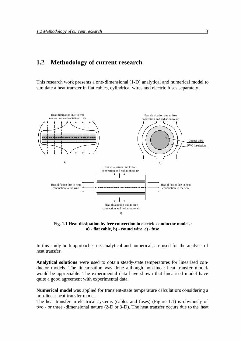
1.2 Methodology of current research This research work presents a one-dimensional (1-D) analytical and numerical model to simulate a heat transfer in flat cables, cylindrical wires and electric fuses separately.
a) b)Heat dissipation due to free
convection and radiation to air
Heat difusion due to heatconduction to the wire
Heat difusion due to heatconduction to the wire
Heat dissipation due to freeconvection and radiation to air
Heat dissipation due to freeconvection and radiation to air
Heat dissipation due to freeconvection and radiation to air
c)
Copper wire
PVC insulation
Fig. 1.1 Heat dissipation by free convection in electric conductor models:
a) - flat cable, b) - round wire, c) - fuse In this study both approaches i.e. analytical and numerical, are used for the analysis of heat transfer. Analytical solutions were used to obtain steady-state temperatures for linearised con-ductor models. The linearisation was done although non- linear heat transfer models would be appreciable. The experimental data have shown that linearised model have quite a good agreement with experimental data. Numerical model was applied for transient-state temperature calculations considering a non- linear heat transfer model. The heat transfer in electrical systems (cables and fuses) (Figure 1.1) is obviously of two - or three -dimensional nature (2-D or 3-D). The heat transfer occurs due to the heat

4 Chapter 1. Introduction diffusion from fuse to the wire or to the fuse holder; also the heat is dissipated from the surfaces of conductors to the ambient due to temperature differences. However, due to the complexity of the numerical model and large time scale of heat transfer processes in the cables it is not computationally efficient to use three-dimensional models to simu-late heat transfer in electrical systems. The CPU time for simulating the same physical system using two- or three -dimensional models is significantly longer than required by a simplified 1-D model. In creating a mathematical model of flat cables (Figure 1.1a) we regard heat transfer only in y – direction (see three-dimensional drawing) while side effects are negligible. Boundary conditions are symmetrical and convective-radiative. Here, convection is assumed unforced and laminar. Flat cable has insula-tion/conductor/insulation layer sequence, where the insulation is PolyVinylChloride (PVC) and the conductor is copper. Insulation layer is described by heat conductivity, specific heat capacity and heat dissipation coefficient. Conductor layer is heated with uniform volumetric heat, generated by electrical current. In the case of cylindrical wires (Figure 1.1b), the 3-D problem is reduced to 1-D regard-ing only radial heat transfer and as infinite length of the wire. The same material proper-ties and boundary conditions apply as for flat cable. The fuse model (1.1c) can also be considered as a cylindrical conductor, only with finite length and without insulation. The model is also reduced to a 1-D model neglecting ra-dial heat transfer, because the fuse element has very high heat conductivity. Since the fuse element has finite length, axial heat transfer is modelled with prescribed tempera-tures on the boundaries T(0,t) and T(L,t). These temperatures are known from wire tem-peratures determined earlier. Due to the non-linear behaviour of material properties with respect to the temperature, a numerical algorithm had to be applied. A finite volume (FV) method was used to ap-proximate partial derivatives of heat transfer equation. The obtained system of non-linear algebraic equations was solved by iterative Newton-Raphson method in order to find nodal unknowns of temperatures in the conductors. The final step of this work was the evaluation of numerical simulation results by the polynomial fitting procedure using the least square (LS) algorithm. A number of mathematical methods have been proposed [10,11,12,13,14] for the analysis of heat transfer in electrical conductors. Usually these methods are pure-analytical or numeri-cal. Analytical methods are easy to handle, physically meaningful but of limited appli-cation for complicated models (non- linear, non-homogenous) and boundary conditions. A numerical approach enables us to implement more realistic boundary conditions, which can be applied to complicated geometries. In order to understand physical mean-ing of the results received from the numerical simulation, calculation results have to be described by simple mathematical equations with as small a number of unknown vari-ables as possible. Therefore, thermo-electrical characteristics of electrical conductors are analysed by polynomial or logarithmical functions. The second reason of derivation of simplified equations is to implement these formulas into computer tool, where a very good time-efficiency can be achieved.

1.3. Scientific novelty 5
1.3 Scientific novelty The special scientific contribution of this work is the particular way to combine analyt i-cal and numerical methods to calculate the thermal behaviour of electrical conductors. The proposed algorithm is based on the following steps: 1. Analytical derivation of the heat transfer equations.
2. Analytical solution of the obtained differential equations with mainly tem-perature independent or linear dependent physical constants. 3. Simplification of the obtained analytical solution to reduce the number of variables. 4. Numerical approximation of the heat transfer equations with non- linear tem-perature dependent phys ical constants. 5. Model validation of the numerical results by experimental data. 6. Interpolation (fitting) of the received numerical results with the simplified equations derived from the analytical solution of the heat transfer equations. 7. Evaluation of the results to receive a limited amount of independent constants (e.g. temperature) to describe the thermal-electrical characteristics with suffi-cient accuracy.
In this study, for the first time, a methodology of heat transfer analysis in electric sys-tems for mobile applications has been formulated. It is shown that it is possible to de-scribe main thermo-electrical characteristics by simplified quasi-analytical functions, which are valid for one particular conductor type. Obtained thermo-electrical characteristics of electrical conductors are:
- thermo – electrical characteristic ∆T(I) :
( ) 20 IbIaIIT +=≤∆
(1.1) - heating-up time characteristic tg(I) :
( )20
2
2
00 lnII
IIIt
−=> τ
(1.2)
- time constant characteristic τ(I) :

6 Chapter 1. Introduction
25.0 IdIcI +−= ττ (1.3)
Having the relationship between the conductor temperature and electrical current (Eq. 1.1), voltage drop in the conductor can be calculated as following:
- voltage drop per length characteristic E(I) :
A
TTI
AI
E))(1( 2
0 ∆+∆+== ρρ βαρρ
(1.4) here: ∆T conductor temperature difference against environment in K I current in A I0 nominal current in A a,b,c,d constants t heating up time in s τ0 nominal time constant in s τ current dependent time constant in s τI time constant at zero current in s E voltage drop per length in V/m ρ specific resistance (resistivity) in Ωm ρ0 specific resistance at reference temperature (e.g. 20°C) in Ωm αρ linear temperature coefficient of the specific resistance in 1/K
βρ square temperature coefficient of the specific resistance in 1/K2
A conductor cross sectional area in m2
In this work an algorithm is proposed to describe thermo-electrical characteristics with the simplified equations (see above 1.1-1.4), which were obtained from analytical and numerical models. This algorithm is suited for implementation in the computer aided cable design program. Based on the proposed algorithm to calculate thermo-electrical characteristics a com-puter program to design electrical systems in cars has been written [15].
1.4 Research approval and publications Created methodology and algorithms, which have been developed to calculate thermo-electrical characteristics of electrical cables for car applications were implemented by cable harness manufacturer Leoni Bordnetzsysteme GmbH and DaimlerChrysler AG. The basic achievements of present research have been presented at the following inter-national conferences:

1.4. Research approval and publications 7
- The 7th International Conference “Electronics’2003” in Kaunas, Lithuania, 2003; - The 8th International Conference “Mathematical Modelling and Analysis” in
Trakai, Lithuania, 2003 The content of the dissertation includes three scientific publications: the two papers are published in the journal “Mathematical Modelling and Analysis” and one publication in “Electronics and Electrical Engineering”. Both journals are edited in Lithuania by an international editorial board.
________________
CHAPTER 2 ________________ PHYSICAL MODELS
OF CONDUCTORS AND THEIR HEAT TRANSFER
EQUATIONS
2.1 Overview Before the discussion of the theoretical model, a short “guide” will be presented at first. This “guidance” is intended to show concisely in what steps the heat transfer equations are going to be developed. It will also be discussed how these equations are solved for cable rating problems. After a short introduction to the model geometry, heat transfer equations of different model geometries will be derived. These equations describe the temperature behaviour in electrical conductors and fuses. As a next step, the heat convection and radiation coefficients will be determined. The heat convective coefficient is presented for cylindrical and horizontal surfaces. Because of its nonlinearity, this coefficient will have to be linearized for the later analytical analysis of the heat equation. Following this, the main physical material parameters of the heat equation will be con-sidered. Because of its non- linearity (e.g. heat conductivity and electrical resistance) in reality, certain simplifications have to be introduced. It will be shown that these simpli-fications can be tolerated for the thermal analysis of the electrical conductor and do not restrict the validity of the simplified thermal conductor model in the temperature range of interest. Finally, required boundary conditions will be introduced. They have to be linearized in order to implement them into an analytical solution of the heat equation. With these preparations, it will be possible to investigate the thermo-electrical charac-teristics of conductors and calculate their ratings.

10 Chapter 2. Physical models of conductors and their heat transfer equations
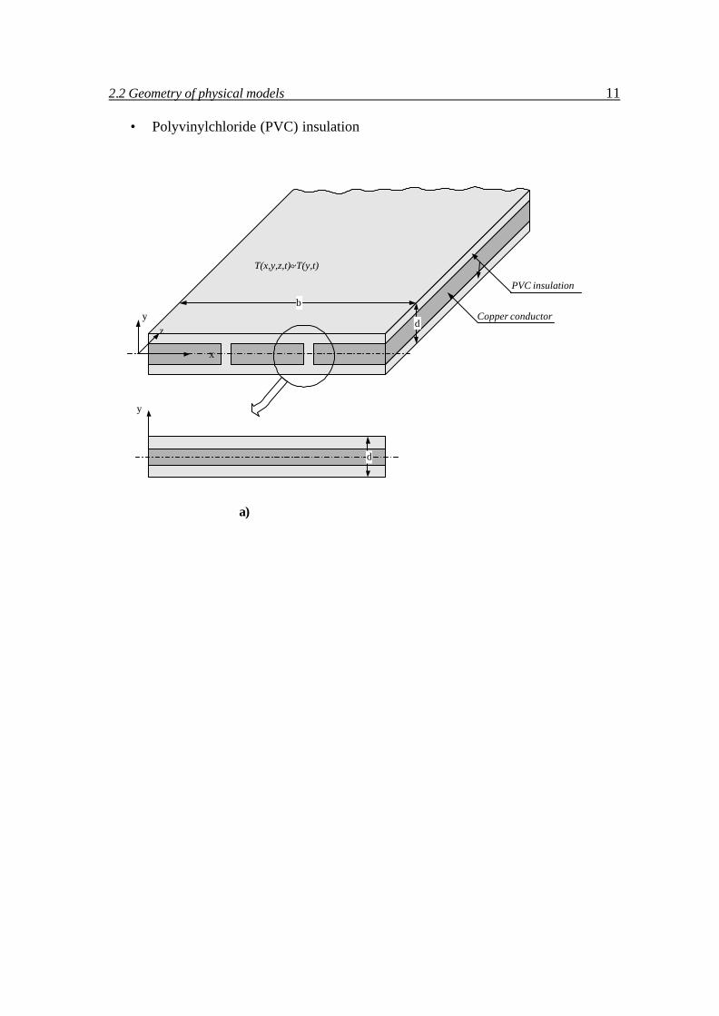
2.2 Geometry of physical models On the basis of electrical conductors, three different models will be considered:
flat insulated cable, round insulated wire, and electrical fuse.
These three different types of conductors cover the main part of power supply system in many applications. In the flat cable model, the term “cable” is used because it has more than one wire. All models are one – dimensional systems, because the other dimensions in all cases vanish due to large difference between cross-sections (for a round wire or fuse) or thickness (for flat cable) and length of the conductors. A. The flat cable model (Fig. 2.1,a) is reduced to one-dimensional heat conduction, whereby spatial derivatives with respect to x and z are neglected:
( 0(...)(...) ≡∂=∂ zx ).
The reduction of the model is possible because of infinite length of the cable L and much bigger width b compared to the thickness d. Due to lateral symmetry of this model, it is sufficient to analyse the upper part of the flat cable only. The model consists of three layers and can be extended depending on the flat cable structure. From “bot-tom” to “top” in the figure (2.1,a) we have:
• Polyvinylchloride (PVC) insulation • Metallic conductors (pure copper) • Polyvinylchloride (PVC) insulation
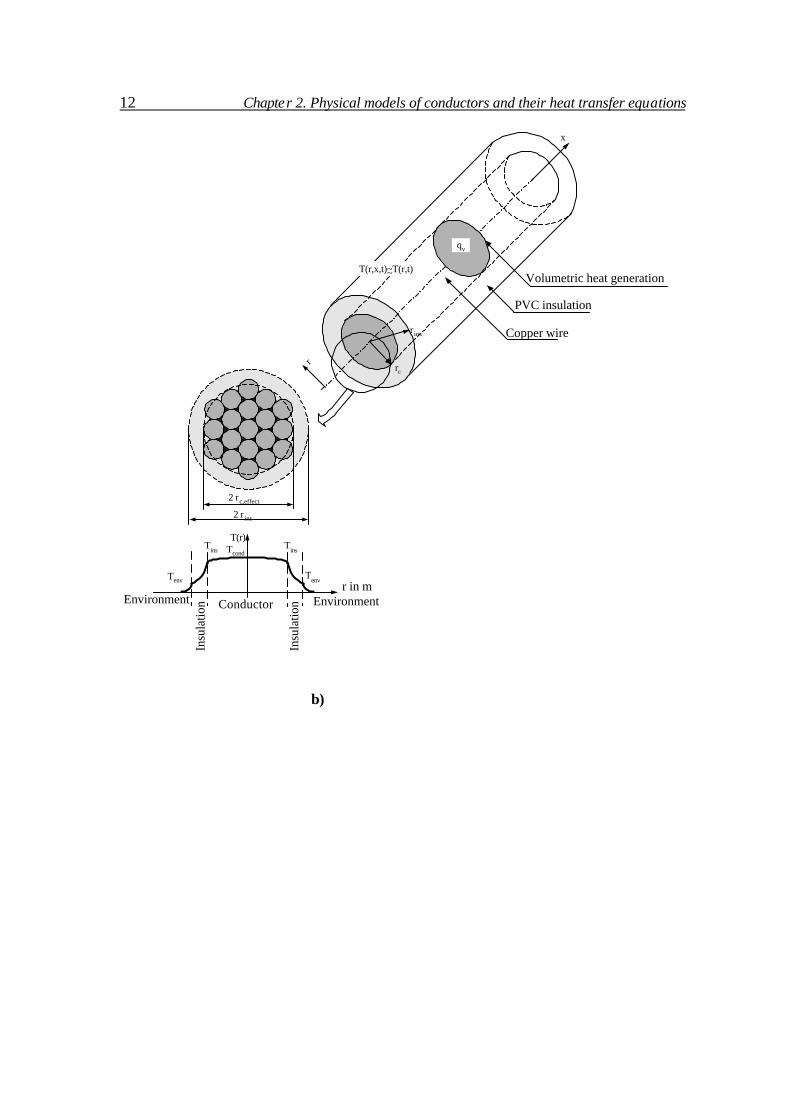
For the sake of simplicity, the conductors (the middle layer) are considered as a homo-geneous conductor layer. B. In round wire model (Fig. 2.1, b) all spatial derivatives of the heat equation vanish with respect to x and ϕ :
( 0(...)(...) ≡∂=∂ ϕx ). The heat conduction in the axial direction is neglected, because normally the length of the wire is much larger than its area, therefore, the boundary effects can be neglected. The angular dimension ϕ is also neglected due to rotational symmetry of the conductor and insulation layer. The whole model consists of two layers and can be extended to more layers, depending on the wire construction. In this model, we have:
• Metallic conductor (98% copper)
2.2 Geometry of physical models 11
• Polyvinylchloride (PVC) insulation
yz
x
d
b
T(x,y,z,t)~T(y,t)~
Copper conductor
PVC insulation
y
d
a)
12 Chapter 2. Physical models of conductors and their heat transfer equations
2 r ins
2 rc,effect
r
r ins
rc
Copper wire
PVC insulation
T(r,x,t)~T(r,t)~ Volumetric heat generation
x
Tenv r in m
Environment
Insu
latio
n Conductor
Insu
latio
n Environment
Tins TcondTins
Tenv
T(r)
qv
b)

2.3 Conservative form of the heat transfer equations 13
Wire
Fuse holderelement 1 Fuse element Wire
Fuse holderelement 2
y
x
Wire
T
Fuse holderelement 1
Fuse holderelement 2
Wire
Temperature T1
Temperature T2
Max.TemperatureTmax
xFuse element
c) Fig. 2.1 Model geometries and heat conduction parameters: a – flat cable, b – round wire, c
– electric fuse The metallic conductor is assumed homogeneous and a perfect cylinder. In reality, the core of wire is made of a number of single conductors with small air gaps in between. If single conductors are arranged symmetrically, then the wire has a hexagonal shape. C. The electrical fuse model is one – dimensional (Fig. 2.1, c) with the heat conduction only along the x – axis. The heat conduction in y – direction is not considered because of very high heat conductivity of copper compared to the heat convection from the sur-face. The shape of the fuse model in x – direction is non-homogeneous. The whole model consists of one layer – copper, bras or any other alloy.
2.3 Conservative form of the heat transfer equations In order to calculate heat dissipation (heat conduction, convection and radiation), the relevant heat transfer equations have to be solved. These equations define the relation-ship between the heat generated by electrical current in metallic conductor, and the tem-perature distribution within the wire or cable (conductor and insulation) and in its sur-roundings.

14 Chapter 2. Physical models of conductors and their heat transfer equations The analysis of heat transfer is governed by the law of conservation of energy. We will formulate this law on a energy rate basis; which means, that at any instant, there must be a balance between all power rates, as measured in Joules (= Ws). The energy conser-vation law can be written in following form:
outstent WWWW +=+ int (2.1) where:
Went is the rate of energy entering the electrical conductor. This energy may be generated by other cables or wires located in the vicinity of other cables or by solar energy, Wint is the rate of heat generated internally by Joule losses, Wst is the rate of energy stored within the cable, Wout is the rate of energy which is dissipated by conduction, convection, and ra-diation.
The inflow and outflow terms Went and Wout are surface phenomena, and these rates are proportional to the surface area. The thermal energy generation rate Wint is associated with the rate of conversion of electrical energy to thermal energy and is proportional to the volume. The energy storage is also a volumetric phenomena, but it is simply associ-ated with an increase (Wst > 0) or decrease (Wst < 0) in the energy of cable. Under steady-state conditions, there is, of course, no change in energy storage (Wst = 0). A de-tailed derivation of the heat transfer equation is given in Appendix A. From the Equation (2.1), (see also Appendix A) general form of the heat transfer equa-tion in conservative form 1in Cartesian (2.2) and cylindrical (2.2a) coordinates is ob-tained as follows [11]:
tT
qzT
zyT
yxT
x v ∂∂
=+
∂∂
∂∂
+
∂∂
∂∂
+
∂∂
∂∂
γρλλλ (2.2)
tT
qT
rrT
rrrx
Tx V ∂
∂=+
∂∂
∂∂
+
∂∂
∂∂
+
∂∂
∂∂
γρφ
λφ
λλ2
11 (2.2a)
here: ? heat conductivity in W/mK qV volumetric heat generation in W/m3
1The conservative form is a form of heat conduction equation where space dependant thermal conductiv-ity or other coefficients remains conserved within different media of materials. The conservative form is given as
∂∂
∂∂
=∂∂
xT
xTT
λγ and the nonconservative form as xT
xxT
tT
∂∂
∂∂
+∂∂
=∂∂ λ
λγ2
2

2.3 Conservative form of the heat transfer equations 15 γ specific heat capacity in W/kgK ρ density in kg/m3
The heat equations (2.2, 2.2a) are the basis for future heat transfer analysis in electrical conductors.
2.3.1 Flat cables
The heat transfer equation (2.2) for flat cable (Fig. 2.1, a), which is derived (in Appen-dix A.1) is simplified for one-dimension as follows:
),(),(
),(),(
),( Tyqt
tyTTy
ytyT
Tyy V=
∂∂
+
∂
∂∂∂
− ργλ (2.3)
As mentioned in the Chapter 2.3, in this model it is considered middle symmetry (Fig.2.2). This assumption is allowed because heat convection and radiation from “top” side of the cable surface has almost the same heat dissipation rate as from the “bottom” side of the cable. It is important to emphasize, that the free convection in air situation is considered. The cable is placed horizontal in the air. In order to simplify the model, the metallic conductor is treated as a homogeneous body across the cable width d (see Fig. 2.1,a). Here, the heat conductivity coefficient λ is space dependant, due to different material layers in the wire. The specific heat capacity term γ is a non-linear function of temperature for copper and PVC insulation. The heat generation by electrical current is expressed as qv term and is called volumetric specific heat flux. It is a linear function of temperature in metallic conductor and vanishes in PVC insulation.
y
x
Insulation Metallic conductor
0
Fig. 2.2 Flat cable model with homogeneous metallic conductor

16 Chapter 2. Physical models of conductors and their heat transfer equations Here, in the equation (2.3), volumetric heat flux is expressed as:
[ ])20(1 20220
22
2
22
−+==⋅⋅
=⋅⋅
== TA
IJ
dlAIdl
dlAIdR
dVdQ
q elV α
ρρ
ρ (2.4)
here
ρel specific resistance of the metallic conductor given by
[ ])20(1 2020 −+= Tel αρρ in Om,
ρ20 specific resistance of the conductor at 20°C temperature α20 copper temperature coefficient at 20°C in 1/K
(α20 = 3.83. 10-3 1/K) l length of the cable in m J current density in A/m2
I denotes current through the wire in A A area of metallic conductor in m2.
2.3.2 Round wires Heat transfer in round wires is determined, in principle, by the same equation as (2.3), heat transfer in radial direction must also be considered. The general form of heat equa-tion in cylindrical coordinates is:
),(),(
),(),(1
),(1
2
TrqtT
Tr
xT
Trx
TTr
rrT
rTrrr
V=∂∂
+
∂∂
∂∂
+
∂∂
∂∂
+
∂∂
∂∂
−
ργ
λφ
λφ
λ (2.5)
Taking into account the model simplifications given earlier (see Fig. 1,b), the heat equa-tion is reduced to the one-dimensional form (see also Appendix A.2):
),(),(
),(),(
),(1
Trqt
trTTr
rtrT
rTrrr V=
∂∂
+
∂∂
∂∂
− ργλ (2.6)
The temperature profile in flat cables and round wires shown in Figure (2.1,a,b) under assumption, that the temperature gradient in a metallic conductor is very small due to its very high heat conductivity. In the insulation the temperature gradient is much larger. The main temperature drop, however, is between the wire surface and environment. This temperature drop is caused by convection and described by heat convection coeffi-

2.4 Physical material constants 17 cient α. Therefore, here it is very important to determine this coefficient correctly. This problem will be discussed in the section 2.5.
2.3.3 Electric fuses
The following differential equation for the heat transfer in the fuse element is given (Appendix, A.3):
[ ]
)()(),(
)()(
)),(()(),(
)( 44
TqxAt
txTxAT
uTtxTTTx
txTxA
x
V
envrc
=∂
∂+
⋅−+∆+
∂∂
∂∂
−
ργ
ααλ (2.7)
here: A cross section area of the fuse element in m2
αc, αr convection and radiation coefficients respectively u circumference in m
envTtxTT −=∆ ),( in K
According to the model (Fig. 2.1,c), the heat transfer should be analysed only in the x direction, because of the short lengths of the fuse melting element. The mathematical model of fuse element should calculate melting temperature of the fuse. Here, radial heat conduction can be neglected due to high heat conductivity of the fuse material. In equation (2.8) the heat flux qV is derived in the same way as in equation (2.5). In ad-dition to this, the equation is valid also for a variable cross sectional area. 2.4 Physical material constants Heat transfer equation given in section 2.3 depends on the specific resistance, heat con-ductivity and the heat capacity of the conductor material. All three values are tempera-ture dependent, however their values are only known for certain temperatures. In order to interpolate between these given values, a linear or square function has to be used to describe the relationship. This estimation is very important in order to model the heat transfer qualitative ly. Different calculation precision criteria are defined for the analytical approach and for the numerical approach. For the analytical approach it is necessary to have temperature independent or linear dependent constants. The numerical approach of the heat transfer model allows more precise temperature calculation in the conductors. Here, non- linear functions can be implemented for the description of the material constants.

18 Chapter 2. Physical models of conductors and their heat transfer equations The following diagrams show the exact graphical and numerical coefficients of the spe-cific resistance, ρ, of copper, of the heat conductivity, ?, of pure copper and PVC, and of the specific heat capacity, γ, of pure copper and PVC [16]. The temperature range in the diagrams is very wide, although in this work only temperature up to 200°C has been considered. The reason of this high temperature range in the charts is to show the over-view how the coefficients behave within wide temperature range. Linear and non- linear approximation has been made using the available data.
273 373 473 573 673 773 873 973 1073 1173 1273 1373
1,50E-008
2,00E-008
2,50E-008
3,00E-008
3,50E-008
4,00E-008
4,50E-008
5,00E-008
5,50E-008
Cu
Spec
ific
resi
stiv
ity ρ
in Ω
m
Absolute temperature T in K
a)
273 373 473 573 673 773 873 973 1073 1173 1273370
375
380
385
390
395
400
405
Cu
Ther
mal
con
duct
ivity
λ in
W/m
K
Absolute temperature T in K
b)

2.4 Physical material constants 19
273 373 473 573 673 773 873 973 1073 1173 1273 1373
375
380
385
390
395
400
405
410
415
420
425
430
435
440
445
Cu
Spec
ific
heat
γ in
J/k
gK
Absolute temperature T in K
c)
Fig. 2.3 Values of: (a) specific resistance, (b) thermal conductivity and (c) specific heat capacity of pure copper
Heat conductivity and specific heat capacity values of PVC:
Temperature in °C Name of material DIN code
20 50 100 Thermal heat conductivity ? in W/Km
Polyvinylchloride PVC 0.17 0.17 0.17 Specific heat capacity γ in J/kgK
Polyvinylchloride PVC 960 1040 1530
Tab 2.1. Values of thermal conductivity and heat capacity of PVC Approximation of the temperature dependent copper and PVC material coefficients: a) Specific resistance of copper ρ:
( ) ( )[ ]2000 1 TTTT −+−+= ρρ βαρρ
here: ρ0 specific resistance at 20°C, ρ0 = 1.75.10-8 in Om αρ linear temperature coefficient, αρ = 4.00.10-3 in 1/K ßρ square temperature coefficient. ßρ = 6.00.10-7 in 1/K2 T temperature of the conductor in °C

20 Chapter 2. Physical models of conductors and their heat transfer equations T0 – reference temperature. In this study reference temperature coincides with environment temperature Tenv . b) specific heat capacity of copper γ:
Tγαγγ += 0 , CT °≤≤ 2000 here: γ0 heat capacity at 20°C reference temperature, γ0 = 381 in J/kgK αγ approximated linear temperature coefficient of heat capacity in 1/K
αγ = 0.17 1/K c) specific heat capacity of PVC γ:
20 TT γγ βαγγ +−= CT °≤≤ 1000
here: γ0 heat capacity at 20°C reference temperature, γ0 = 920 in J/kgK αγ approximated linear temperature coefficient of heat capacity in 1/K
αγ = 1.3 1/K ßγ approximated square temperature coefficient of heat capacity in 1/K2
ßγ =0.074 1/K2
2.5 Determination of heat transfer coefficients The heat transfer from the surface is governed by convection and radiation. This effect can be described by the corresponding convection and radiation heat transfer coeffi-cients. Both depend on the surface and environment temperatures. Convection takes place between the boundary surface and a heat transport by a fluid (e.g. air) in motion at a different temperature. Radiation occurs by electromagnetic wave heat exchange between the surface and its surrounding environment separated by air. In this work the convective heat transfer coefficient of laminar flow has to be examined for the following two different model geometries:
- horizontal cylinder surfaces - horizontal plate surfaces
The result of this examination leads to two different heat transfer coefficients valid for round and for plate surfaces. The convection and radiation coefficient appears in the boundary conditions of the heat transfer equations for the electrical conductor models. At the lower temperatures, which are typical for electric cable applications, convection is the basic heat dissipation component (ca. 90%).
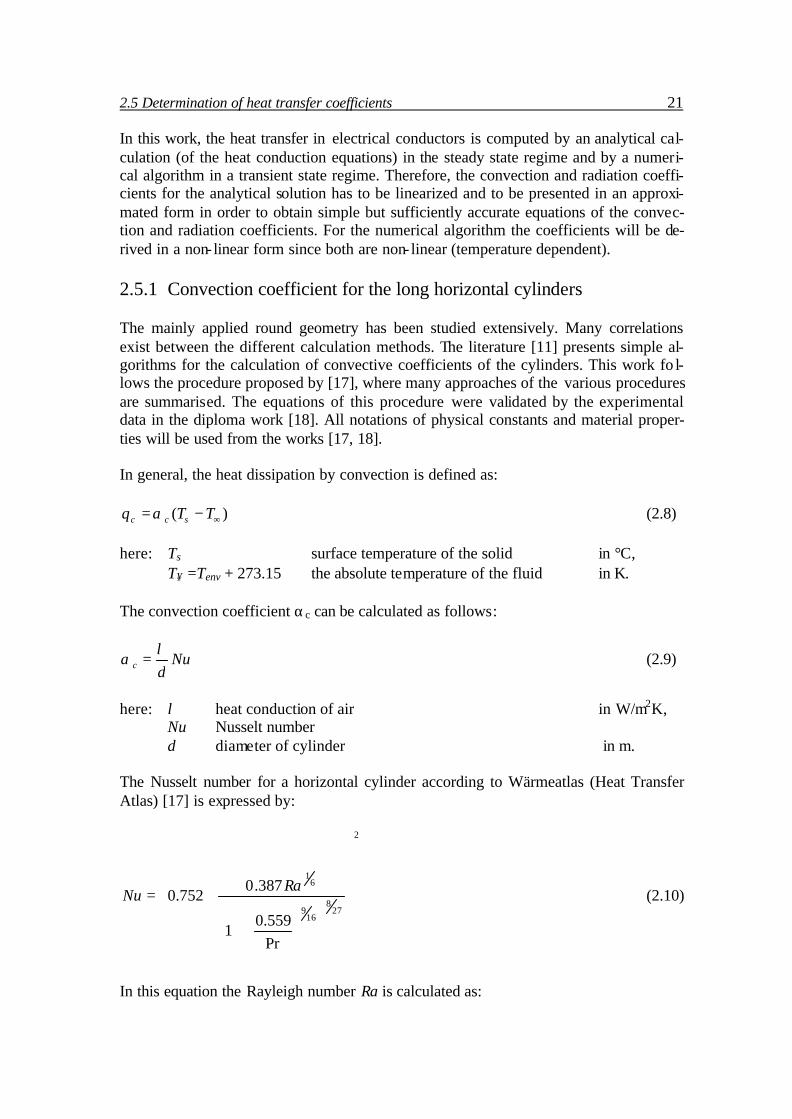
2.5 Determination of heat transfer coefficients 21 In this work, the heat transfer in electrical conductors is computed by an analytical cal-culation (of the heat conduction equations) in the steady state regime and by a numeri-cal algorithm in a transient state regime. Therefore, the convection and radiation coeffi-cients for the analytical solution has to be linearized and to be presented in an approxi-mated form in order to obtain simple but sufficiently accurate equations of the convec-tion and radiation coefficients. For the numerical algorithm the coefficients will be de-rived in a non- linear form since both are non- linear (temperature dependent). 2.5.1 Convection coefficient for the long horizontal cylinders The mainly applied round geometry has been studied extensively. Many correlations exist between the different calculation methods. The literature [11] presents simple al-gorithms for the calculation of convective coefficients of the cylinders. This work fo l-lows the procedure proposed by [17], where many approaches of the various procedures are summarised. The equations of this procedure were validated by the experimental data in the diploma work [18]. All notations of physical constants and material proper-ties will be used from the works [17, 18]. In general, the heat dissipation by convection is defined as:
)( ∞−= TTq scc α (2.8) here: Ts surface temperature of the solid in °C,
T∞ =Tenv + 273.15 the absolute temperature of the fluid in K. The convection coefficient αc can be calculated as follows:
Nudcλ
α = (2.9)
here: λ heat conduction of air in W/m2K,
Nu Nusselt number d diameter of cylinder in m.
The Nusselt number for a horizontal cylinder according to Wärmeatlas (Heat Transfer Atlas) [17] is expressed by:
2
278
169
61
Pr559.0
1
387.0752.0
+
+=Ra
Nu (2.10)
In this equation the Rayleigh number Ra is calculated as:

22 Chapter 2. Physical models of conductors and their heat transfer equations Ra = Gr Pr (2.11) Here: Pr Prandtl number (see Tab. 2.2) and
Gr Grashof number defined by the following equation:
2
3 )(v
TTgdGr ∞−
=β
, (2.12)
here: g gravitational acceleration in m/s2, ß volumetric thermal expansion coefficient in 1/K, ν kinematic viscosity in (m2/s). The ß coefficient for ideal gas with justifiable error can be considered as:
∞
=T1
β (2.13)
where T∞ =Tenv + 273.15 - the absolute temperature of the fluid (in K) The material constants λ, ν and Pr of air are taken from Heat Transfer Atlas [17]. These constants are dependent on the average temperature Tave:
)(21
envsave TTT += (2.14)
here Ts is temperature of the surface of cylinder (in °C) and Tenv – environment tempera-ture (in °C). With the equations (2.9) and (2.10), the convection coefficient αc is written as follows:
2
278
169
61
Pr559.0
1
387.0752.0
+
+=Ra
dcλ
α (2.15)
Replacing in the equation (2.15) the Rayleigh number Ra, the Prandl number Pr and heat conductivity λ leads to the following form, which is only diameter d and tempera-ture difference ∆T dependant:
( )2
61
1
21
1
1
∆+
= TK
dK Tdcα
(2.16)

2.5 Determination of heat transfer coefficients 23
where: 21
1 752.0 λ=dK , (2.17) and
6
1
227
816
9
21
1Pr
Pr559.0
1
387.0
+
=vg
KTβλ
(2.18)
The physical constants of air i.e. (heat conductivity λ, kinematic viscosity ν and the Prandtl number Pr) can be found in the literature [17]. For the volumetric thermal ex-pansion coefficient ß, air is considered as an ideal gas. For reference, environment tem-perature is taken. In the table 2.2 Kd1 and KT1 values for a temperature range from 20 to 140°C are given. Surface tempera-ture T in °C
Temperature Tave in °C
Heat conducti v-ity λ in 10-3 W/mK
Kinematic viscosity ν in 10-6 m2/s
Prandtl number Pr
Kd1 KT1
20 20 25.67 15.35 0.7147 0.1205 1.1121 40 30 26.41 16.29 0.7133 0.1222 1.1054 60 40 27.14 17.25 0.7121 0.1239 1.0990 80 50 27.87 18.23 0.7110 0.1255 1.0928 100 60 28.58 19.24 0.7100 0.1271 1.0868 120 70 29.29 20.26 0.7091 0.1287 1.0810 140 80 30.00 21.31 0.7083 0.1302 1.0754 Average: 0.1254 1.0932
Tab 2.2. Physical constants of air for temperature from 20 to 140 °C The averaged form of the convective coefficient for temperature range from 20 to 140°C is following:
( )2
612
1
1.09321
0.1254
∆+
= T
dcα
(2.19) 2.5.2 Convection coefficient for horizontal plates For the application for flat cables the free convection of horizontal plates has been con-sidered as well. For this geometry, we have to distinguish between the convection from the top side of the plate surface and the bottom side.

24 Chapter 2. Physical models of conductors and their heat transfer equations The convection coefficient αc is calculated similar to equation (2.9):
Nulcλ
α = (2.20)
here l is characteristic length, which is defined as:
PA
l ≡ ,
where A and P are the plate surface and perimeter, respectively. A. The Nusselt number for the upper side of horizontal plate according to Wärmeatlas (Heat Transfer Atlas) [17] is expressed by: a. For laminar flow:
51
2011
2011
Pr322.0
1766.0
+=
−
RaNu , (2.21)
here: 4
1120
2011
107Pr322.0
1 ⋅≤
+
−
Ra .
b. For turbulent flow:
31
2011
2011
Pr322.0
115.0
+=
−
RaNu (2.22)
here: 4
1120
2011
107Pr322.0
1 ⋅≥
+
−
Ra .
B. The Nusselt number for the lower side of a horizontal plate has the following form (only laminar convection):

2.5 Determination of heat transfer coefficients 25
51
916
169
Pr492.0
16.0
+=
−
RaNu (2.23)
here 10
916
169
3 10Pr492.0
110 <
+<
−
Ra
All the equations (2.1, 2.13) and Nusselt numbers given in (2.21, 2.22, 2.23) are in-serted into equation (2.20). This leads to the following form of the convection coeffi-cients: A. Upper side a. Laminar flow:
( ) 513
8
211
Tl
KTc ∆
=α
(2.24) here:
51
2011
2011
221 Pr322.0
1Pr
766.0
+=
−
vg
KTβ
λ (2.25)
b. Turbulent flow:
( ) 31
22 TlKTc ∆=α (2.26)
here: 3
120
1120
11
222 Pr322.0
1Pr
15.0
+=
−
vg
KTβ
λ (2.27)
B. Lower side (laminar flow only):
( ) 513
8
311
Tl
KTc ∆
=α
(2.28) here:

26 Chapter 2. Physical models of conductors and their heat transfer equations
51
916
169
231 Pr322.0
1Pr
6.0
+=
−
vg
KTβ
λ (2.29)
2.5.3 Exact mathematical expressions of the physical constants of air The physical constants of air depend very much on temperature. These functions are of higher polynomial order, which were obtained by fitting of the given results in the Wärmeatlas [17]. With these functions, a very high accuracy of convection coefficient can be achieved and the function can easily be implemented into the computer program. Here, the wide temperature range is used in order to expand the validity range of tem-perature dependent constants in the computer program. A. Heat conductivity in air λ (Tave): Temperature range for the fitting procedure: CTC ave °≤≤°− 1000200 Obtained polynomial function by fitting:
414311285 1099059.11036064.4103282.41061617.702416.0
)(
aveaveaveave
ave
TTTT
T−−−− ⋅−⋅+⋅−⋅+
=λ
(2.30)

2.5 Determination of heat transfer coefficients 27
-200 0 200 400 600 800 1000
0
10
20
30
40
50
60
70
80
90
Data according to Heat Atlas [17] Empirical function (Polynom 4.Grade)
Hea
t con
duct
ivity
of a
ir λ
in 1
0-3 W
m-1K
-1
Temperature Tave in °C
Fig. 2.4 Heat conductivity of air as a function of temperature at constant pressure P = 105 Pa
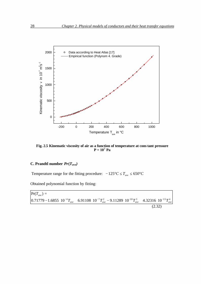
B. Kinematic viscosity ν (Tave): Temperature range for the fitting procedure: CTC ave °≤≤°− 1000200 Obtained polynomial function by fitting:
41731421085 1064882.1106463.41014171.11082402.81035391.1
)(
aveaveaveave
ave
TTTT
T−−−−− ⋅+⋅−⋅+⋅+⋅
=ν
(2.31)
28 Chapter 2. Physical models of conductors and their heat transfer equations
-200 0 200 400 600 800 1000
0
500
1000
1500
2000 Data according to Heat Atlas [17] Empirical function (Polynom 4. Grade)
K
inem
atic
vis
cosi
ty ν
in
10-7 m
2 s-1
Temperature Tave
in °C
Fig. 2.5 Kinematic viscosity of air as a function of temperature at cons tant pressure P = 105 Pa
C. Prandtl number Pr(Tave) Temperature range for the fitting procedure: CTC ave °≤≤°− 650125 Obtained polynomial function by fitting:
413310274 1032316.41011289.91091108.6106855.171779.0
)Pr(
aveaveaveave
ave
TTTT
T−−−− ⋅+⋅−⋅+⋅−
=
(2.32)

2.5 Determination of heat transfer coefficients 29
-200 0 200 400 600 800 10000.68
0.70
0.72
0.74
0.76
0.78
0.80
0.82
0.84
0.86
0.88
650°C-120°C
Empirical funktion (Polynom 4.Grade)for Temperature range -120°C < T
ave < 650°C
Data according to Heat Atlas [17]
P
rand
tl-nu
mbe
r P
r
Temperature Tave in °C
Fig. 2.6 Prandtl-number of air as a function of temperature at constant pressure P = 105 Pa
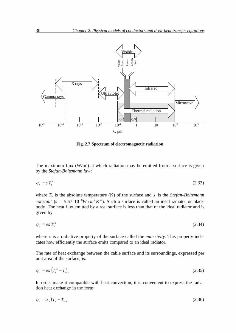
2.5.4 Radiation In order to describe heat transfer by the thermal radiation in electrical conductors, the exchange of radiation energy between the insulated conductor surface and the infinitely large environment is considered. It may occur not only from solid surfaces but also from liquids and gases [11]. The en-ergy of the radiation is transported by electromagnetic waves (or alternatively, photons). While the transfer of energy by conduction or convection requires the presence of a ma-terial medium, radiation does not. In fact, radiation transfer occurs most efficiently in a vacuum. The complete electromagnetic spectrum is shown in Figure 2.7. The short wavelength gamma rays, X rays and ultraviolet (UV) radiation are primarily of interest to the high energy physicist and nuclear engineer, while the long wavelength micro-waves and radio waves are of concern to the electrical engineers. It is the intermediate portion of the spectrum, which extends from approximately 0.1 to 100 µm. It includes a part of the UV and all of the visible infrared (IR), that is called thermal radiation and belongs to heat transfer.
30 Chapter 2. Physical models of conductors and their heat transfer equations
10-5 10-4 10-3 10-2 10-1 1 10 102 103
Gamma rays
X rays
Thermal radiation
0.4 0.7
Microwave
InfraredUltraviolet
Voi
let
Blu
e
Gre
en
Yel
low
Red
Visible
λ, µm
Fig. 2.7 Spectrum of electromagnetic radiation
The maximum flux (W/m2) at which radiation may be emitted from a surface is given by the Stefan-Boltzmann law:
4sr Tq σ= (2.33)
where TS is the absolute temperature (K) of the surface and σ is the Stefan-Boltzmann constant ( 428 /1067.5 KmW−⋅=σ ). Such a surface is called an ideal radiator or black body. The heat flux emitted by a real surface is less than that of the ideal radiator and is given by
4sr Tq εσ= (2.34)
where ε is a radiative property of the surface called the emissivity. This property ind i-cates how efficiently the surface emits compared to an ideal radiator. The rate of heat exchange between the cable surface and its surroundings, expressed per unit area of the surface, is:
( )44envsr TTq −= εσ (2.35)
In order make it compatible with heat convection, it is convenient to express the radia-tion heat exchange in the form:
( )envsrr TTq −= α (2.36)

2.6 Boundary conditions 31 where from Equation (2.35) the radiation heat transfer coefficient αr is:
( )( )22
envsenvsr TTTT ++≡ εσα (2.37)
Here we have modelled the radiation in the same way as convection. In this sense we have linearised the radiation rate equation, making the heat rate proportional to a tem-perature difference rather than to the difference between two temperatures to the fourth power. Note, however, that αr depends strongly on temperature, while the temperature dependence of the convection heat transfer coefficient αc is generally weak. Since the free convection and radiation transfer occurs simultaneously, the convection and radiation has to be added. Then the total rate of heat transfer from the surface is as follows:
)()( 44envsenvscrc TTTTqqq −+−=+= εσα (2.38)
The total heat transfer by convection and radiation expressed as the heat transfer coeffi-cient α is:
( )( )22envsenvscrc TTTT +++=+= εσαααα
(2.39)
2.6 Boundary conditions In order to have a unique solution of the PDE (partial differential equation), boundary and initial conditions have to be specified as shown below. In case of differential equa-tions for the electrical fuse, prescribed boundary conditions are used. PDE’s of flat and round electrical cables will have symmetry and non-linear convective-radiative bound-ary conditions. 1. Flat electrical cable
- initial condition
)()0,( yTyT env= (2.40)
32 Chapter 2. Physical models of conductors and their heat transfer equations - boundary conditions
( )( ) ( )
−+−∆=∂∂
−
=∂
∂
=
→
.,
,0),(
lim
44
0
envenvyy
y
TTTTTlyT
ytyT
N
εσαλ
λ
(2.41)
2. Round electrical wire - initial condition
)()0,( rTrT env= (2.42)
- boundary conditions
( )( ) ( )
−+−∆=∂∂
−
=∂
∂
=
→
.,
,0),(
lim
44
0
envenvrr
r
TTTTTdrT
rtrT
r
N
εσαλ
λ (2.43)
3. Electrical fuse - initial condition
)()0,( xTxT env= (2.44)
- boundary conditions
=
=
)(),(
)(),0(
2
1
tTtxT
tTtT (2.45)
The boundary and initial conditions in equations (2.40-2.45) are generally valid and im-plemented into the numerical algorithm of heat transfer calculations. In the analytical analysis of heat transfer (Chapter 3), some additional boundary cond i-tions will be used to solve the PDE of flat cables and round wires. Here we have to cal-culate with the constant heat transfer coefficient and do not take into account the non-linear phenomena of radiation. The following additional boundary conditions apply for a flat electrical cable:

2.6 Boundary conditions 33
−−=
+−=
=
=
)(
,)(2
1
0
envinsyy
insyy
TTdydT
bdEI
dydT
λα
λ (2.46)
In case of cylindrical wire:
−−=
−=
=
=
)(
,2
1
0 0
envinsrr
insrr
TTdrdT
rEI
drdT
λα
λπ (2.47)

________________
CHAPTER 3 ________________
ANALYTICAL ANALYSIS
OF HEAT TRANSFER IN A STEADY STATE
In the preceding Chapter 2, a definition of heat transfer equations for the study of ana-lytical and numerical heat transfer computation was given. The objective of those equa-tions is to determine the temperature field in different kinds of electrical conductors where heat conduction, convection/radiation and energy generation takes place. Differ-ent boundary conditions were also given for the solutions of those equations. The aim of the present chapter is to obtain exact analytical solutions in a steady-state regime. Because of the linearization of differential equations, some difference between numerical and analytical results will occur, but these mismatches can be accepted in many situations. It is always convenient to have a simple analytical solution if a steady state is required. The following assumptions are made to simplify the partial differential equations: a) steady-state conditions, b) one-dimensional conduction, c) constant or linear material properties, d) uniform volumetric heat generation, e) constant heat transfer coefficient.
3.1 Calculation of the thermo-electrical characteristics of flat cables 3.1.1 Vertical heat transfer with temperature-independent coefficients For pure vertical heat transfer in flat cables equation (2.6, Chapter 2) will be used:
),()()( yTqtT
TyT
yy V=
∂∂
+
∂∂
∂∂
− ργλ (2.6)
Considering assumptions for the heat equation made before we get the following equa-tion:
36 Chapter 3. Analytical analysis of heat transfer in a steady state
( ) ( )0
,,2
2
=∂
∂−+
∂∂
ttyT
AEI
ytyT
λγρ
λ (3.1)
or,
( ) ( )0
,,2
2
=∂
∂−+
∂∂
ttyT
DCy
tyT (3.2)
here: 2
2
AI
AEI
Cλρ
λ=≡ ;
λγρ
≡D .
3.1.2 Vertical heat transfer with temperature-dependent coefficients Considering specific resistance ρ and electrical field strength E dependence on tempera-ture:
[ ])),((1)( 0 envTtyTT −+= ραρρ (3.3)
[ ])),((1)( 0 envTtyTETE −+= ρα (3.4) here: αρ linear temperature coefficient of resistance in 1/K ρ0 specific resistance at reference temperature T0 in °C E0 field strength at reference temperature T0 in °C Then, equation (3.2) obtains this form:
( ) ( )[ ] ( )0
,,1
, 02
2
=∂
∂−∆++
∂∂
ttyT
tyTA
IEy
tyTλγρ
αλ ρ
( ) ( ) ( )0
,,
, 002
2
=∂
∂−+∆+
∂∂
ttyT
AIE
tyTA
IE
ytyT
λγρ
λλ
α ρ (3.5)
or,
( ) ( ) ( )0
,,
,2
2
=∂
∂−+∆+
∂∂
ttyT
DCtyTBy
tyT
(3.6)

3.1 Calculation of the thermo-electrical characteristics of flat cables 37 Since in equation (3.6) the term with B is temperature dependant, steady state can only be reached if additional conditions are satisfied. The necessity of such a condition arises from the fact that the specific resistance ρ increases with temperature. The solution of temperature change in time can be presented in the following form:
∑∞
=
+=
1
2sin)(),(j
j d
dy
jtgytT π (3.6b)
This result is recognised as a Fourier sine-series expansion of the arbitrary function Tj(y), for which the constant amplitudes gj are given by:
∫
+=
d
ij ydyd
dy
jyTd
tg0
2sin)(2
)( π . (3.6c)
Only, if 2
2
dB
π< the solution of steady state temperature exist.
here: A
IEB
λ
α ρ 0≡ ; AIE
Cλ
0≡ ; λγ
≡D ; TBC ˆ1
=≡ρα
; envTtyTT −=∆ ),( .
3.1.3 Stationary solution of vertical heat transfer equation The stationary solution will be obtained for rectangular cables, namely, flat cables, where the cable width b is much larger than the thickness d. This solution describes the temperature pattern in a metallic conductor of a flat cable and its insulation in vertical y direction. Three different cases of electrical conductor are considered, for which a stationary solu-tion of the heat equation is achieved: A) Cable without insulation and temperature-dependent specific resistance ρ ( 0≠B ),
Dirichlet boundary conditions; B) Cable without insulation and temperature- independent specific resistance ρ ( 0=B ),
symmetry and convective boundary conditions; C) Cable with insulation and temperature-independent specific resistance ρ ( 0=B ), symmetry and convective boundary conditions. Case A. Cable without insulation and temperature-dependent specific resistance ρ
( 0≠B ).

38 Chapter 3. Analytical analysis of heat transfer in a steady state The heat equation (3.6) for steady-state simplifies to:
( ) ( ) 02
2
=+∆+∂
∂CyTB
yyT
(3.7)
The general solution of equation (3.7) is:
BC
yBTyBTyT'
21 cossin)( −+= (3.8)
here T1,2 – integration constants in °C and CBTC env −=' . In order to get a temperature profile, boundary conditions for the equation (3.8) have to be applied. The temperatures are fixed at the boundary (Dirichlet conditions) at the bot-tom side of the flat cable (y=-d/2) and upper side - (y=d/2). For y=-d/2:
Td
BTd
BTTd
T ˆ2
cos2
sin2 2101 ++−==
− (3.9a)
For y=d/2:
Td
BTd
BTTd
T ˆ2
cos2
sin2 2102 ++==
(3.9b)
This leads to the integration constants T1,2:
2sin2
0011 d
B
TTT
−= (3.10a)
2cos2
ˆ20102 d
B
TTTT
−+= (3.10b)
The insertion of integration constants into the general solution (3.8) gives the following temperature distribution in the flat cable:
TyBd
B
TTTyB
dB
TTyT ˆcos
2cos2
ˆ2sin
2sin2
)( 02010102 +−+
+−
=
(3.11)

3.1 Calculation of the thermo-electrical characteristics of flat cables 39 here: d – thickness of the cable, T01- boundary temperature at y=-d/2, T02-boundary tem-perature at y=d/2. For T01 = T02 equation (3.11) can be simplified:
yBd
B
TTTyT cos
2cos
ˆˆ)( 01−
−=
(3.12) Case B. Cable without insulation and temperature-independent specific resistance ρ
( 0=B ) In case the temperature dependence of the specific resistance can be neglected, the equation (3.2) simplifies to:
( )0
,2
2
=+∂
∂C
ytyT
(3.13)
The general solution of this equation (3.13) is:
212
2)( TyTy
CyT ++−= (3.14)
where T1 and T2 are integration constants. Symmetry and convective boundary conditions (Fig.3.1) are applied:
y
d
0),(
lim0
=∂
∂→ y
tyTy
λqv
( ) ( )( )envdy
ins TTbddydT
bd −+=+−=
22 222
αλ
d1
-d1x
Fig. 3.1 Boundary conditions considering temperature gradient in conductor only of flat cable

40 Chapter 3. Analytical analysis of heat transfer in a steady state
at y=0: 00
=∂∂
=yyT
; and (3.15)
at y=d1 : ( ) ( ) )(22 11
1
envdy
TTbdyT
bd −+−=∂∂
+=
αλ , or
)(2
envdy
TTyT
−−=∂∂
= λα
. (3.16)
The relationship (3.16) is developed by applying a surface energy balance. Here the heat transfer coefficient is considered constant. Substituting the appropriate rate equations (3.13, 3.14, 3.15 and 3.16) temperature pro-file in the conductor of flat cable is obtained:
( ) 11
21
22
1 21
2)( d
bdEI
Tdy
dC
yT env +++
−=
α (3.17)
( ) 11
21
22
1 21
2)( d
bdEI
Tdy
dC
yT env +++
−=
α
here: C Case C. Cable with insulation and temperature- independent specific resistance ρ
( 0=B )
For the calculation of the temperature distribution in an insulated flat cable (case C), the boundary conditions should be applied to the borders of the insulation (see Fig.3.2). Due to high thermal conductivity of the conductor compared to the insulation, the tem-perature gradient in the metallic conductor can be assumed to be zero. Applying as overall energy balance law to the flat cable model, we obtain following boundary cond i-tions:
y
d
qv
( ) EIdydT
bddy
ins =+−= 1
12λ
( ) ( )( )envdy
ins TTbddydT
bd −+=+−=
22 222
αλ
d2
d1
-d2
-d1x
Fig. 3.2 Boundary conditions considering temperature gradient in the insulation alone of flat cable

3.1 Calculation of the thermo-electrical characteristics of flat cables 41 at y = d1:
( ) EIdydT
bddy
ins =+−= 1
12λ , or insdy bd
EIdydT
λ)(2 11+
−==
; (3.18)
at y = d2:
( ) ( )( )envdy
ins TTbddydT
bd −+=+−=
22 222
αλ , or ( )envinsdy
TTdydT
−−== λ
α
2
(3.19)
The equation (3.7) can be written as follows
( )0
2
2
=∂
∂y
yT (3.20)
which by integration becomes:
1TyT
=∂∂
(3.21)
where T1 is a integration constant. Taking into account the limit condition (3.18) the constant T1 is:
( )bdEI
Tins +
−=1
1 2λ
The temperature Tins of the outer surface of the insulation, according to (3.19) is given by:
( )bdEI
TT envins ++=
22α (3.22)
The temperature profile in the insulation body can be determined by integrating the equation (3.21):
( )y
bdEI
TyTins
ins ++=
22)(
λ (3.23)

42 Chapter 3. Analytical analysis of heat transfer in a steady state Temperature at the inner side of insulation, which also means temperature of metallic conductor is given with y=d1:
( ) 112
dbd
EITT
insinsc +
+=λ
(3.24)
or, expressed as a function of environment temperature Tenv:
( ) ( ) 112 22
ybd
EIbd
EITT
insenvc +
++
+=λα
(3.25
3.2 Calculation of thermo-electrical characteristics of round wires
3.2.1 Radial heat transfer with temperature-independent coefficients
For radial heat transfer we consider infinite length cylindrical wire thus neglecting end effects. This assumption is reasonable if the ratio of cylinder length L and cylinder ra-dius r is L/r ≈ 1000. The general heat equation for radial system is:
( ) ( )0
,,1=
∂∂
−+
∂∂
∂∂
ttrT
AEI
rtrT
rrr λ
γλ
(3.26)
or,
( ) ( )0
,,1=
∂∂
−+
∂∂
∂∂
ttrT
DCr
trTr
rr
(3.27)
here: 2
2
AI
AEI
Cλρ
λ=≡ ;
λγ
≡D
3.2.2 Heat transfer equations with temperature-dependent coefficients Here the specific resistance dependence on temperature will be considered:
[ ])),((1)( 00 TtrTT −+= ραρρ (3.28)

3.2 Calculation of thermo – electrical characteristics of round wires 43 The electrical field strength E changes with temperature as following:
[ ])),((1)( 00 TtrTETE −+= ρα (3.29) here: αρ - linear temperature coefficient of resistance ρ0 – specific resistance at reference temperature T0 E0 – field strength at reference temperature T0
Then the equation (3.27) obtains the following form:
( ) ( )[ ] ( )0
,,1
,1 0 =∂
∂−∆++
∂∂
∂∂
ttrT
trTA
IEr
trTr
rr λγ
αλ ρ
( ) ( ) ( )0
,,,1 00 =∂
∂−+
∆+
∂∂
∂∂
ttrT
AIE
A
trTIE
rtrT
rrr λ
γλλ
α ρ (3.30)
or,
( ) ( ) ( )0
,,
,1=
∂∂
−+∆+
∂∂
∂∂
ttrT
DCtrTBr
trTr
rr
(3.31)
here: A
IEB
λ
α ρ 0≡ ; AIE
Cλ
0≡ ; λγ
≡D .
3.2.3 Stationary solution of radial heat transfer equation Before solving the equations, a short explanation of the applications shall be given where the solutions are applicable. Again, first the heat equation will be solved for the “naked” wire i.e. cylindrical wire without insulation (Fig. 3.1a). In this case, tempera-ture distribution occurs only in the metallic conductor. Secondly, the heat equation will be applied to the round wire with insulation (Fig. 3.1b). Here the temperature distribu-tion will be calculated whilst the insulation layer while temperature gradient of the me-tallic conductor is assumed to be zero. For steady state and constant material properties, the heat transfer equation reduces to B = 0:
( )0
1=+
∂∂
∂∂
CrrT
rrr
(3.32)
44 Chapter 3. Analytical analysis of heat transfer in a steady state
Insulation
Conductor
r2
r1
T
T0
Tc
Tins
Ter
-r1-r2 0 r2r1
T(r)
Conductor
r1
T
T0
Tc
Te
r0-r1 r1
T(r)
a) b)
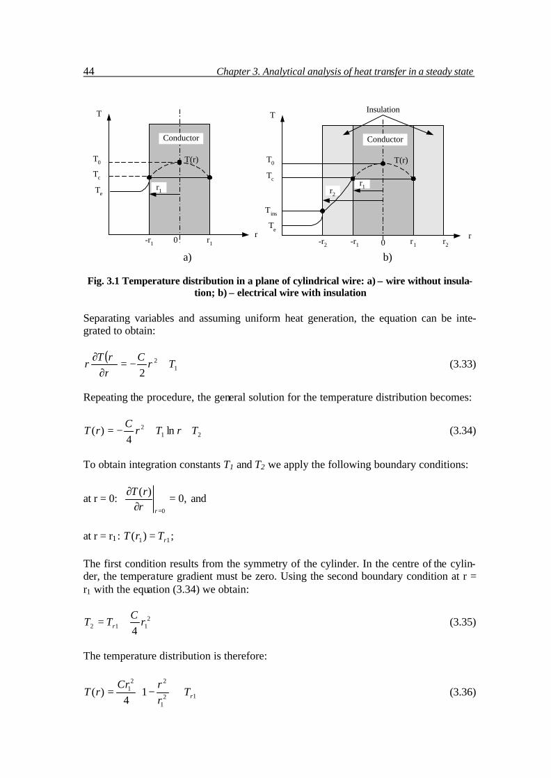
Fig. 3.1 Temperature distribution in a plane of cylindrical wire: a) – wire without insula-tion; b) – electrical wire with insulation
Separating variables and assuming uniform heat generation, the equation can be inte-grated to obtain:
( )1
2
2Tr
CrrT
r +−=∂
∂ (3.33)
Repeating the procedure, the general solution for the temperature distribution becomes:
212 ln
4)( TrTr
CrT ++−= (3.34)
To obtain integration constants T1 and T2 we apply the following boundary conditions:
at r = 0: ,0)(
0
=∂
∂
=rrrT
and
at r = r1 : 11)( rTrT = ; The first condition results from the symmetry of the cylinder. In the centre of the cylin-der, the temperature gradient must be zero. Using the second boundary condition at r = r1 with the equation (3.34) we obtain:
2112 4
rC
TT r += (3.35)
The temperature distribution is therefore:
121
221 1
4)( rT
rrCr
rT +
−= (3.36)
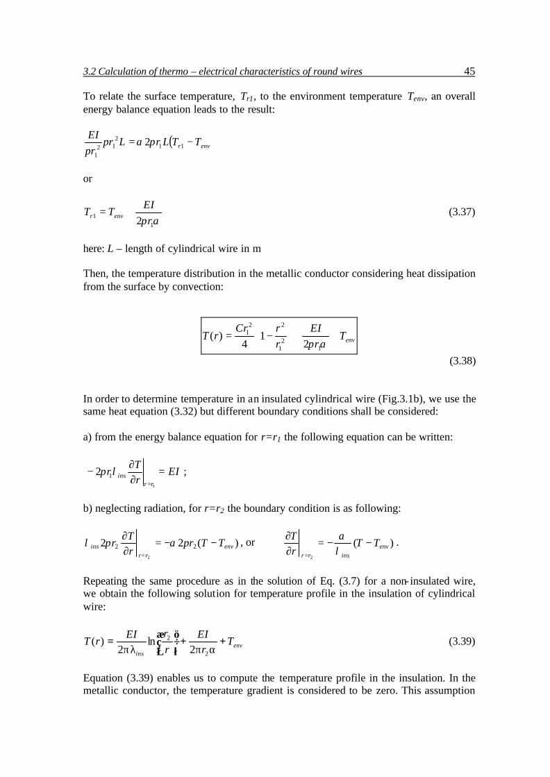
3.2 Calculation of thermo – electrical characteristics of round wires 45 To relate the surface temperature, Tr1, to the environment temperature Tenv, an overall energy balance equation leads to the result:
( )envr TTLrLrr
EI−= 11
212
1
2παππ
or
απ 11 2 r
EITT envr += (3.37)
here: L – length of cylindrical wire in m Then, the temperature distribution in the metallic conductor considering heat dissipation from the surface by convection:
envTr
EIrrCr
rT ++
−=
απ 12
1
221
21
4)(
(3.38) In order to determine temperature in an insulated cylindrical wire (Fig.3.1b), we use the same heat equation (3.32) but different boundary conditions shall be considered: a) from the energy balance equation for r=r1 the following equation can be written:
EIrT
rrr
ins =∂∂
−= 1
12 λπ ;
b) neglecting radiation, for r=r2 the boundary condition is as following:
)(22 22
2
envrr
ins TTrrT
r −−=∂∂
=
παπλ , or )(2
envinsrr
TTrT
−−=∂∂
= λα .
Repeating the same procedure as in the solution of Eq. (3.7) for a non- insulated wire, we obtain the following solution for temperature profile in the insulation of cylindrical wire:
envins
Tr
EIrrEI
rT ++
=
αππλ 2
2
2ln
2)( (3.39)
Equation (3.39) enables us to compute the temperature profile in the insulation. In the metallic conductor, the temperature gradient is considered to be zero. This assumption

46 Chapter 3. Analytical analysis of heat transfer in a steady state is reasonable, because the heat conductivity of a metallic conductor is very high, com-pared with the insulation heat conductivity. Temperature of metallic conductor at r=r2 from Eq. (3.39) is therefore:
envins
c Tr
EIrrEI
T ++
=
αππλ 21
2
2ln
2
(3.40)
3.3 Calculation of the thermo-electrical characteristics of
electrical fuses 3.3.1 Axial heat transfer with temperature – independent coefficients For the analytical analysis of axial heat transfer we will use similar equation to (Eq. 2.8, Chapter 2) and introduce temperature- independent coefficients. Then the equation has the form:
0),(
),(),(
2
2
=∂
∂−+−
∂∂
ttxT
AEI
txTAu
xtxT
λγ
λλα
(3.41)
here: BAu
≡λα
; CA
EI≡
λ; D≡
λγ
.
Then equation (3.41) can be rewritten following:
0),(),(
2
2
=∂∂
−+−∂
∂tT
DCtxBTx
txT
(3.42) Let us describe the coefficient phys ical meaning of equation (3.42). These coefficients do not depend on temperature. Coefficient B can be written in the following form:
2
1χλ
α=≡
Au
B (3.43)

3.3 Calculation of thermo – electrical characteristics of electrical fuses 47 here χ - is the “length constant”, e.g. the inversed square root of coefficient B :
uA
B αλ
χ =≡1
(3.44)
χ can be considered as a length decay in a function of temperature, which increases if the ratio A / u increases. Coefficient C is called “Temperature field gradient” in K/m2. The coefficient means the ratio of the volumetric generated heat EJ in the fuse and the heat conductivity coeffi-cient ? :
λρ
λ
2JA
EIC =≡ (3.45)
We introduce the “asymptotic temperature” termT . Asymptotic term can be understood as a final temperature of infinite length wire after steady state. Temperature T in the fuse will not be achieved if the fuse has a very short length. In any case T will not be reached in transient state. The formula of T is the following:
uEI
CBC
Tα
χ ==≡ 2ˆ (3.46)
Coefficient D can be called “reciprocal temperature conductivity” or “reciprocal heat transport velocity” and is described as the quotient of heat capacity and heat conductiv-ity:
λγ
≡D (3.47)
3.3.2 Axial heat transfer with temperature-dependent coefficients In this section we will consider temperature dependant specific electrical resistance of copper or brass. Specific resistance, ρ, for temperature change from 20 to 180°C can be calculated as follows:
[ ])),((1)( 0 envTtxTT −+= ραρρ (3.48) The field strength, E, changes with respect to temperature as:
[ ])),((1)( 0 envTtxTETE −+= ρα (3.49)

48 Chapter 3. Analytical analysis of heat transfer in a steady state here: αρ linear temperature coefficient of resistance ρ0 specific resistance at reference temperature T0 E0 field strength at reference temperature T0
Considering Eq. (3.49), equation (3.41) takes the following form:
[ ]0
),()),((1),(
),( 02
2
=∂
∂−
−++−
∂∂
ttxT
A
TtxTIEtxT
Au
xtxT env
λγ
λ
α
λα ρ
( ) 0),(
),(),( 00
2
2
=∂
∂−+−
−−
∂∂
ttxT
AIE
TtxTA
IEu
xtxT
env λγ
λλ
αα ρ (3.50)
or,
( ) 0),(),(
2
2
=∂∂
−+−−∂
∂tT
DCTtxTBx
txTenv
where the coefficients have the following meaning:
0
1IEu
AB ραα
λχ
−=≡ (3.51)
envTIEu
EIC
BC
T +−
==≡0
2ˆραα
χ (3.52)
3.3.3 Avalanche effect in metallic conductor Any conductor with a positive temperature coefficient αρ shows a so-called avalanche effect, where due to too larger energy generation, the equilibrium, generated between energy in the fuse and dissipated heat to ambient can not be achieved. This is valid for the length constant as well as for the final temperature of a wire with infinite length. Because of this effect, temperature rises continuously and the length constant χA and final temperature AT becomes infinite if the following conditions are satisfied:
A
IIEu
20
0
ρααα ρ
ρ ==
(3.53)

3.3 Calculation of thermo – electrical characteristics of electrical fuses 49 Then: ∞=∞= AA T,χ Avalanche current can be calculated in this way:
0ραα
ρ
uAI A =
(3.54) 3.3.4 Stationary solution for axial heat transfer equation The solution of the equation for axial heat transfer gives the temperature distribution in the x – direction. For steady-state we apply boundary conditions given in equation (2.46, Chapter):
=
=
lTxT
TT
)(
)0( 0 (2.46)
Then, the equation (3.42) of axial heat transfer simplifies to:
0)()(
2
2
=+∆−∂
∂CxTB
xxT
(3.55)
The general solution of Eq. (3.55) is:
BC
eTeTxT xBxB'
21)( −+= − (3.56)
here: B linear temperature dependent heat dissipation coefficient to ambient in 1/m2 CBTC env −=' temperature dependent heat generation by electrical current in 1/m2 T1,2 integration constants, in which the boundary conditions are set in °C In order to find T1,2 we introduce boundary values at x = 0 and x = l. Then, the tempera-ture distribution in the fuse is as following:

50 Chapter 3. Analytical analysis of heat transfer in a steady state
( ) ( )Te
e
TeTeTe
e
TeTeTxT xB
lB
lBl
lBlxB
lBl
lBlBˆ
1
1ˆ
1
1ˆ)(
20)(
20 +
−
−+−−
−
−+−−= −
−
−−−
−
−−
(3.57)
here: l length of fuse in m T(x) temperature distribution along the fuse in °C T0 the boundary temperature of the fuse at x = 0 in °C Tl the boundary temperature of the fuse at x = l in °C
Replacing B by2
1χ
, equation (3.17) can be written as:
Te
e
TeTeT
e
e
TeTeT
xTx
l
l
l
l
lx
l
l
ll
ˆ
1
1ˆ
1
1ˆ
)( 2
0
2
0
+
−
−+
−
−
−
−+
−
−=−
−
−−
−
−
−−
χ
χ
χχ
χ
χ
χχ
(3.58) Equation 3.58 gives the temperature distribution in a fuse element with the finite length and fixed boundary temperatures. From the analytical solution the “avalanche effect” (Eq. 3.52) can be observed, the length constant χ is obtained (Eq.3.51), and “hypotheti-cal temperature” T can be derived (Eq. 3.52).

________________
CHAPTER 4 ________________
NUMERICAL CALCULATION OF TEMPERATURE BEHAVIOUR
IN A TRANSIENT STATE
4.1 Overview of the numerical methods used in heat transfer computation
The heat transfer of an insulated electrical wire is described by a non-linear and non-homogeneous partial differential equation. A unique analytical solution is only feasible for idealised and simple conditions. For practical cases, it is required to implement nu-merical methods. Available analytical and experimental results are of considerable im-portance in verifying the accuracy and validity of numerical results. The limitations of an analytical solution arise from the following properties of electrical wires:
• electrical conductivity is second order temperature dependent • heat conductivity λ of insulation is at least linear temperature dependent • heat convection and radiation α is at least third order temperature dependant
The numerical methods allow not only better representation of the mutual heating ef-fects, but also permit more accurate modelling of the boundaries (e.g. a convection-radiation boundary to the environment). A numerical solution is obtained from discretisation of the partial differential equation. There are four distinct streams of numerical solution techniques:
• Finite Differences (FD) • Finite Element (FE) • Spectral Method (SM) • Finite Volume Method (FV)
The four mentioned methods differ mainly in the approximation of the variables and in the discretisation processes.
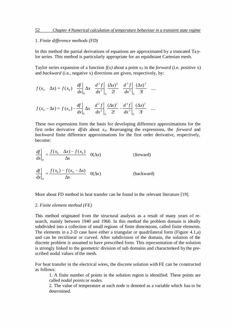
52 Chapter 4 Numerical calculation of temperature behaviour in a transient state regime 1. Finite difference methods (FD) In this method the partial derivations of equations are approximated by a truncated Tay-lor series. This method is particularly appropriate for an equidistant Cartesian mesh. Taylor series expansion of a function f(x) about a point x0 in the forward (i.e. positive x) and backward (i.e., negative x) directions are given, respectively, by:
....!3)(
!2)(
)()(3
03
32
02
2
000 +
∆+
∆+∆+=∆+
xdx
fdxdx
fdx
dxdf
xfxxf
....!3)(
!2)(
)()(3
03
32
02
2
000 +
∆−
∆+∆−=∆−
xdx
fdxdx
fdx
dxdf
xfxxf
These two expressions form the basis for developing difference approximations for the first order derivative df/dx about x0. Rearranging the expressions, the forward and backward finite difference approximations for the first order derivative, respectively, become:
)(0)()( 00
0
xx
xfxxfdxdf
∆+∆
−∆+= (forward)
)(0)()( 00
0
xx
xxfxfdxdf
∆+∆
∆−−= (backward)
More about FD method in heat transfer can be found in the relevant literature [19]. 2. Finite element method (FE) This method originated from the structural analysis as a result of many years of re-search, mainly between 1940 and 1960. In this method the problem domain is ideally subdivided into a collection of small regions of finite dimensions, called finite elements. The elements in a 2-D case have either a triangular or quadrilateral form (Figure 4.1,a) and can be rectilinear or curved. After subdivision of the domain, the solution of the discrete problem is assumed to have prescribed form. This representation of the solution is strongly linked to the geometric division of sub domains and characterised by the pre-scribed nodal values of the mesh. For heat transfer in the electrical wires, the discrete solution with FE can be constructed as follows: 1. A finite number of points in the solution region is identified. These points are called nodal points or nodes. 2. The value of temperature at each node is denoted as a variable which has to be determined.

4.1 Overview of the numerical methods used in heat transfer computation 53 3. The solution region is divided into a finite number of subregions called ele ments. These elements connect common nodes, and collectively approximate the shape of the region. 4. Temperature is approximated over each element by a polynomial expression that is defined using nodal values of the temperature (see Fig. 4.1, b): mjiP CBAT ωωω ++= where ωi, ωj, ωm are the area coordinates defined as in Fig. 4.1, b. These area coordinates uniquely define the position of any point P inside the triangle ijm. A different polynomial is defined for each element, but the element polynomials are selected in such a way that continuity is maintained along the element boundaries. The nodal values are computed so that they provide the “best” approximation possible to the true temperature distribution. This selection is ac complished by minimising some quantity associated with the physical prob lem or by using Galerkin’s method [29], which deal with the differential equa tions directly. The solution vector of the algebraic equations gives the required nodal temperatures. The answer is then known throughout the solution region. More about FE method can be found in literature [20].
a) b)
Fig. 4.1 Triangular or quadrilateral finite elements of a two-dimensional domain (a) and area coordinates (b)
3. Spectral method Spectral methods approximate the unknowns by means of truncated Fourier series or series of Chebyshev polynomials. Unlike the finite difference or finite element approach the approximations are not local but valid throughout the entire computational domain. The unknowns in the governing equation are replaced by the truncated series. The con-strain that leads to the algebraic equations for the coefficients of the Fourier or Cheby-shev series is provided by a weighted residuals concept similar to the finite element method or by making the approximate function coincide with the exact solution at a
m
ji
ωj
ωm
ωiP
y
x

54 Chapter 4 Numerical calculation of temperature behaviour in a transient state regime number of grid points. Further information on this specialised method can be found in [21] 4. The finite volume method The finite volume method was originally developed as a special finite difference formu-lation [22, 23]. In FV method, the partial derivation of equations is not directly ap-proximated like in FD approach. Instead, the equations are integrated over a control vol-ume V, which is defined by nodes of grids on the mesh:
dVtT
dVqdVTgraddivVV
vV
∫∫∫ ∂∂
=+ γλ )(
The volume integral terms will be replaced by surface integrals using the Gauss for-mula. For a vector a this theorem states:
∫∫ =AV
dAandVadiv .
These surface integrals define the convective and diffusive fluxes through the surfaces. Due to the integration over the volume, the method is fully conservative. This is an im-portant property of FV method. This clear relationship between the numerical algorithm and the underlying physical conservation principle forms one of the main attractions of the finite volume method and makes its concept much simpler to understand by engineers than finite element and spectral methods. In fact, 40 years ago Lax and Wendroff proved mathematically that conservative numerical methods, if convergent, do converge to correct solution of the equation. This study shall be solely concerned with this most well – established and thoroughly validated general-purpose computational fluid dynamic (CFD) and heat transfer technique. Therefore the method is discussed in more detailed.
4.2 Fundamentals of the finite volume method The basic laws of heat transfer are the conservation equations, which are statements that express the conservation of: mass, momentum, and energy in a volume closed by its surface.

4.2 Fundamentals of the finite volume method 55
B1/2 1 i-1 i i+1
T(x)
x
∆x ∆xTi-1 Ti+1 TB
Ti
Figure 4.2 One-dimensional Finite Volume Mesh
Certain requirements are necessary to convert these laws into partial differential equa-tions. These requirements cannot always be guaranteed. In a case where a discontinuity occurs, an accurate representation of the conservation laws is important. In other words, it is of big importance that these conservation equations are accurately represented in their integral form. The most natural method to accomplish this is obviously to discritise the integral form of the equations but not the differential form. This is the basis of finite volume (FV) method. In two dimensional cases the field or domain is subdivided in the same way as in the finite element method, namely, into a set of non-overlapping cells that cover the whole domain on which the equations are applied. On each cell the conservation laws are ap-plied to determine the flow variables in some discrete points of the cells, called nodes, which are typical locations of the cells such cell-centre (cell centered mesh) or cell-vertices (cell vertex mesh) (Figure 4.3). Obviously, there is considerable freedom in the choice of the cell shapes. They can be triangular, quadrilateral etc. and generate a structured or unstructured mesh. Due to this unstructured form, very complex geometries can be handled with ease. This is clearly an important advantage of the method. Additionally the solution of the equation of the cell is not strongly linked to the geometric representation of the domain. This is another important advantage of the finite volume method in contrast to the finite element method.

56 Chapter 4 Numerical calculation of temperature behaviour in a transient state regime
(a) (b)
Figure 4.3 Two-dimensional structured Finite Volume Mesh system:
(a) Cell Centred mesh (b) Cell Vertex mesh
Numerical properties of discretisation schemes. It is normally distinguished between time and spatial discretisation of continuum equa-tion. The spatial discretisation can be applied on different forms of grids such as Carte-sian, non-orthogonal, structured and unstructured. Time discretisation is usually done by FD scheme, which can be explicit or implicit. Normally, the explicit method is used for strong unsteady flows or when time gradient is very big. When a direct computation of the dependent variables can be made in terms of known quantities, the computation is said to be explicit. In contrast, when the dependent variables are defined by coupled sets of equations, and either a matrix or iterative technique is needed to obtain the solution, the numerical method is said to be implicit. The choice of whether an implicit versus explicit method should be used depends ulti-mately on the goal of the computation. The consequences of using both methods have to do with numerical stability and numerical accuracy. Using explicit methods we can achieve required accuracy in time with more computational effort than implicit method. Although, explicit methods are simpler to implement mathematically, they are almost in all cases only conditionally stable. Implicit formulation is said to be always uncondi-tionally stable. A solution for the unknowns at one time level n+1 may be obtained for any size of time step. In computational heat transfer, the governing equations are nonlinear. Under these conditions implicitly formulated equations are almost always solved using iterative techniques. Since heat transfer in electrical conductors has no strong unsteady flows as well as considering efficiency and stability of implicit method,

4.3 Non-linear heat transfer model of electrical conductors 57 whenever possible implicit methods are used in this work but explicit method can be applied optionally. Good understanding of the numerical solution algorithm is crucial. Three mathematical concepts are useful in determining the success or otherwise of such algorithms: conver-gence, consistency and stability. Convergence is the property of a numerical method to produce a solution, which ap-proaches the exact solution as the grid spacing, control volume size or element is re-duced to zero ( 0)(lim
0=−
→ nmeshTT , T – exact solution of partial differential equation, Tn –
solution of finite difference equation). Consistent numerical schemes produce systems of algebraic equations, which can be demonstrated to be equivalent to the original governing equations, as the grid spacing tends to zero. Stability is associated with damping of errors as the numerical method proceeds. If a technique is not stable even round off errors in the initial data can cause erratic oscilla-tions and divergence. Convergence is usually very difficult to establish theoretically and in practice Lax’s equivalence theorem is used [4], which states that for linear problems a necessary and sufficient condition for convergence is that the method is both consistent and stable. In heat transfer calculations this theorem is of limited use since we stated that the govern-ing equations are non- linear. In such problems consistency and stability are necessary conditions for convergence, but not sufficient.
4.3 Non-linear heat transfer model of electrical conductors It has already been mentioned that using the numerical methods the differential and the integral equations can be transformed into discrete algebraic equations. Based on the mentioned reasons in the previous section (4.2), the FV method has been chosen for the discretisation of PDE. Equation (2.2, Chapter 2)
tT
qzT
zyT
yxT
x v ∂∂
=+
∂∂
∂∂
+
∂∂
∂∂
+
∂∂
∂∂
γλλλ (4.1)
can be rewritten in the integral form. We integrate Equation (2.2) over a small fixed volume V:
dVtT
dVqdVTgraddivVV
vV
∫∫∫ ∂∂
=+ γλ )( (4.2)

58 Chapter 4 Numerical calculation of temperature behaviour in a transient state regime The volume integral over the divergence of heat flux vector is transformed to a surface integral by means of the divergence theorem. Then Equation (4.2) becomes
dVtT
dVqdSnTgradVV
vS ∂
∂=+⋅ ∫∫∫ γλ )( (4.2a)
where S is the surface area of the finite volume. Since,
nT
nTgrad∂∂
=⋅ (4.2b)
then, the equation (4.2a) gives:
dVtT
dVqdSnT
VVv
S ∂∂
=+∂∂
∫∫∫ γλ (4.2c)
here: V small finite volume; n outward drawn normal unit vector
n∂
∂ derivative along the outward drawn normal to the surface of the control
volume. Equation (4.2a) represents the principle of conservation of energy over finite volume V. It states that the rate of energy entering the control volume through its boundary surface S plus the rate of energy generated in the volume element is equal to the rate of increase of stored energy in the control volume. Furthermore, since fluxes are conserved in transport between the control volumes, the conservation principle is also satisfied for an assembly of finite volumes. That is, the numerical solution will satisfy both the local and global conservation properties, hence the formulation given by Equation (4.2) is fully conservative.
4.3.1 Approximation of heat transfer equations by FVM
4.3.1.1 Flat electric cable
We consider the transient state diffusion with convective-radiative boundary condition of a flat electrical cable in a one-dimensional domain defined in Figure 4.4.

4.3 Non-linear heat transfer model of electrical conductors 59
yz
x
d
b
T(x,y,z,t)~T(y,t)~
Copper conductor?(T),γ(T)
PVC insulation?(T),γ(T),α(T)
y
d
( )( ) ( )44, envenv
yy
TTTTTlyT
N
−+−∆=∂∂
−=
εσαλ
0),(
lim0
=∂
∂→ y
tyTy
λqv(T)
Air (free convection
and radiation)
Tenv
,α
Figure 4.4 The physical model of flat electrical cable heated by electrical current
It is assumed that the dimensions in the x- and z- directions are so large that temperature gradients are significant in the y- direction only. The used grid is shown in Figure 4.5:
yN1/2 1 i-1 i+1
y
∆y
Ti-1 Ti+1TN
∆y∆y/2
Ti
0 iyc yins
Figure 4.5 The finite volume grid of flat cable The governing equation is:
),(),()( yTqtT
yTyT
yy v=
∂∂
+
∂∂
∂∂
− γλ (4.3)

60 Chapter 4 Numerical calculation of temperature behaviour in a transient state regime The Equation (4.3) models the heat conduction in an electrical wire, which has different materials namely a conductor (here: copper) and an insulator (here: PVC = PolyVinyl-Chloride) with different heat conductivities λ. Moreover, there is no heat generation qv in wire (PVC) insulation. Therefore the equation has discontinuous coefficients λ and qv:
<<==
<<≠=
;;0,
,0;0,
inscvins
cvc
yyyq
yyq
λλ
λλ (4.4)
The integral form of the governing equation for interior nodes of flat cable gives:
∫ ∫ ∫∆ ∆ ∆
=∂∂
+
∂∂
∂∂
−V V V
v dVqdVtT
yTdVyT
yy
),()( γλ (4.5)
Applying this integral form to the finite volume Vi= [i-0.5; i+0.5] (Figure 4.5) the Equa-tion (4.5) can be rewritten whereby the volume element dV is replaced by the surface element dy (using Gauss theorem):
∫∫∫+
−
+
−
+
−
∆=∆∂∂
+
∂∂
∂∂
−5.0
5.0
5.0
5.0
5.0
5.0
),(),()(i
iv
i
i
i
i
ydyyTqydytT
yTdyyT
yy
γλ (4.6)
Integration of the Equation (4.6) over [i-0.5; i+0.5] leads to:
iviii
yyTqtT
yyTyT
yyT
y ∆=∂∂
∆+∂∂
+∂∂
−−+
),(),()()(5.05.0
γλλ (4.7)
Replacing partial derivatives in space by central differences and derivative in time by backward difference, the Equation (4.7) takes the form:
iin
in
iiin
in
ii
ini
ni
i
i yzTqTTt
yTTT
yTT
y∆=−
∆∆
+−∆
+−∆
− −−
−
−+
+
+ ),()()(
)()( 11
5.0
5.01
5.0
5.0 γλλ (4.8)
The partial derivatives Eq. (4.8) in space are of second order accuracy and in time of first order (∆y2,∆t).

4.3 Non-linear heat transfer model of electrical conductors 61 Equation (4.8) is solved implicitly in time. In this study semi- implicit scheme is used, so the time step can not be chosen too large. The space step ∆y and time step ∆t can be computed by these expressions:
5.0−+
=∆N
ddy insc and
Kt
t =∆ (4.8a)
here: t time needed to reach steady state in some yi node, K number of time steps needed to reach steady state regime.
The result of this numerical solution gives temperature distribution in the metallic con-ductor and insulation of the flat cable.
4.3.1.2 Round electric wire
Cylindrical electrical wire of infinite length is given in (Figure 4.6)

62 Chapter 4 Numerical calculation of temperature behaviour in a transient state regime
2 rins
2 rc,effect
Air (free convection and
radiation)Tenv, α
qv
r
rins
rc
Copper wire?(T),γ(T)
PVC insulation
?(T),γ(T),α(T)
T(r,x,t)~T(r,t)~ Volumetric heat generation
x
Figure 4.6 The model of heat conduction in round electrical wire rc – radius of the metallic conductor (copper), rins – radius of the insulation (PVC), rc,effect –
effective radius of the conductor (pure copper without air gaps between single conduc-tors)
In the heat transfer model of cylindrical wire we consider heat conduction in the cross section and neglect the conduction along the wire, assuming, that the end effects of the wire have no influence to the aimed calculation results. This approximation is reason-able for L/rins>1000, where L – length of the wire. The numerical scheme is shown in Figure 4.7:

4.3 Non-linear heat transfer model of electrical conductors 63
1/2 1 i-1 i i+1
r
∆r
Ti-1 Ti+1TN
∆r∆r/2
Ti
rc rins
0 rN
Figure 4.7 The finite volume grid of round wires The governing equation is:
),(),()(1
rTqtT
rTdrdT
rrrr v=
∂∂
+
∂∂
− γλ (4.9)
Equation (4.9) has discontinuous coefficients λ and P:
<<==
≤<≠=
;;0,
,0;0,
inscvins
cvc
rrrq
rrq
λλ
λλ (4.10)
After multiplication of the Equation (4.9) by r, the integral form of the governing equa-tion for interior nodes of cylindrical wire becomes:
∫ ∫ ∫∆ ∆ ∆
=∂∂
+
∂∂
−V V V
v dVrTrqdVtT
rTrdVdrdT
rrr
),(),()( γλ (4.11)
Applying this integral form to the finite volume Vi= [i-0.5; i+0.5] (Figure 4.7) we can rewrite the Equation (4.12) as following:
∫∫∫+
−
+
−
+
−
∆=∂∂
∆+
∂∂
∂∂
−5.0
5.0
5.0
5.0
5.0
5.0
),(),()(i
iv
i
i
i
i
rdrrTrqdrtT
rrTrdrrT
rrr
γλ (4.12)
Integrating over [i-0.5; i+0.5] we get:
ivii
ii
i rrTqtT
rrTrT
rrrT
rr ∆=∂∂
∆+∂∂
+∂∂
−−
−+
+ ),(),()()(5.0
5.05.0
5.0 γλλ (4.13)

64 Chapter 4 Numerical calculation of temperature behaviour in a transient state regime Replacing partial derivatives in space by central differences and derivative in time by backward difference, the Equation (4.13) takes the form:
iiin
in
ii
niin
in
ii
iini
ni
i
ii rqrTTt
rrTT
rr
TTr
r∆=−
∆∆
+−∆
+−∆
− −−
−
−−+
+
++ )()()( 11
2/1
2/12/11
2/1
2/12/1 γλλ (4.14)
Equation (4.14) is solved semi- implicitly in time. The space step ∆r and time step ∆t can be computed by these expressions:
5.0−=∆
Nr
r ins and Kt
t =∆ (4.15)
here: rins the radius of insulated wire, N number of nodes, t the time needed to reach steady state in some yi node, K a number of time steps needed to reach steady state regime.
4.3.1.3 Electric fuse
Here, the problem deals with the axial heat transfer calculation in a copper (or brass) solid or hollow cylinder (fuse melting element prototype) with finite length (Figure 4.8). Axial temperature distribution in the fuse melting element must be computed in order to obtain the maximum temperature (melting temperature) of this element. In the mathe-matical model of heat transfer in the fuse, the non-homogenous geometry, heat convec-tion and radiation is considered through the surface of the fuse element and prescribed temperature boundary conditions are applied. The temperature gradient in the radia l di-rection is neglected, because heat conductivity coefficient of copper (or brass) is very large and gives a constant temperature distribution for the model geometry considered here. This model reduction reduces computational efforts considerably.

4.3 Non-linear heat transfer model of electrical conductors 65
dc
Wire
y
x
Wire
T(x,y,z,t)~T(x,t)~
T(0,t) T(L,t)
Fuse holder element 1 Fuse elementFuse holder element 2
d i
d1d2
d3
Air (free convection and
radiation)Tenv, α
Figure 4.8 Physical model of the fuse melting element used for numerical computation
The heat transfer equation of the energy conservation law for a 1-D problem in the axial direction can be expressed as:
[ ]
)()()(),(
)()()( 44
TqxAtT
xArT
uTTTTxT
xAx
v
envrc
=∂∂
+
⋅−+∆+
∂∂
∂∂
−
γ
ααλ (4.16)
here: αc convection heat transfer coefficient in W/m2K, ∆T temperature difference between the temperature T on the surface and environment temperature Tenv in K, αr = εσ radiation heat transfer coefficient in W/m2K4, u circumference of the fuse element in m, A area (depends on the geometry of the fuse element) in m2. Following the same procedure as in previous sections (4.3.1.1-2) we integrate Eq. (4.16) over [i-0.5; i+0.5] (Fig. 4.9). After integration equation yields:
[ ]
xTqxAdtdT
xxArT
uTTTTdxdT
xAdxdT
xA
v
envrcii
∆=∆+
−+∆++−−+
)()()(),(
)()()()( 44
5.05.0
γ
ααλλ (4.17)
Replacing the derivatives by central differences in space and derivative in time by backward difference, the Equation (4.17) gives:

66 Chapter 4 Numerical calculation of temperature behaviour in a transient state regime
[ ]
iiin
in
iii
ni
niienv
nNr
nenv
nNc
ni
ni
i
iini
ni
i
ii
xqATTt
xA
TuTTTTT
TTx
ATT
xA
∆=−∆
∆+
−+−+
−∆
+−∆
−
−
−−
−−+
+
++
)(
))(())((
)()(
1
44
15.0
5.05.01
5.0
5.05.0
γ
αα
λλ
(4.18)
The space step ∆x and time step ∆t is computed by:
1−=∆
NL
x and Kt
t =∆ (4.19)
here: L length of the fuse element, N number of nodes in which the temperature is calculated, T time needed to reach steady state in some xi node, K number of time steps needed to reach steady state regime.
xN1/2 1 i-1 i+1
x
∆x
Ti-1 Ti+1TN
∆x∆x/2
Ti
i
Figure 4.9 The finite volume grid of fuse
4.3.2. Numerical implementation of boundary conditions
4.3.2.1. Flat electric cable
The mathematical model of heat transfer in the flat cable consists of PDE and two boundary conditions. Therefore, the heat transfer problem must be considered as an ini-tial-boundary value problem. Here we have to deal with mixed-type boundary cond i-tions, which consist of Neumman type boundary conditions (second kind) and convec-tive-radiative limit conditions (third kind). Since the flat cable model is a symmetrical system (see Fig. 4.4), we can use symmetry boundary condition at y = 0. The cable is placed in air in a horizontal position and affected only by laminar free convection and radiation to the environment. Due negligible difference between the heat convection on the upper and lower sides of the cable, this symmetry assumption is correct.

4.3 Non-linear heat transfer model of electrical conductors 67 In this section we show how to approximate this type of boundary condition in order to have the same order of accuracy as the governing equation. Initial and boundary condition is given as:
[ ]
( )( ) ( ) ( )( )
≥−+−=∂
∂−
≥=∂
∂∈=
=
→
0,),(),(,),(
0,0),(
)(lim
,0),()0,(
4*4*
00
tTtyTTtyTTdy
tyT
ty
tyTy
yyyTyT
envenvcyy
N
y
Nenv
N
εσαλ
λ (4.20)
here T*
env is the absolute temperature of environment in K. The first boundary condition, which is derived from the symmetry of the physical model, has to be inserted into the main equation (4.5) and integrated over region [r0; r0.5]:
dyyTqdytT
yTdyyT
yy
y
y
y
y
y
y∫∫∫ =
∂∂
+
∂∂
∂∂
−5.0
0
5.0
0
5.0
0
),(),()( γλ (4.20a)
Following the same procedure as in the derivation of the discrete form of the governing equation (4.8), the following discrete form of the first boundary condition is obtained:
0015.00
15.0
5.0 )()( qyTTt
yTT
yn
in
i
nn
in
i ∆=−∆
∆+−
∆− −
+γλ
(4.20b)
In order to describe heat conduction through the boundary of cable insulation and envi-ronment, we have to integrate Equation (4.3) over the region [yN-0.5;yN]:
dyyqdytT
ydyyT
yy
N
N
N
N
N
N
y
y
y
y
y
y∫∫∫−−−
∆=∂∂
∆+
∂∂
∂∂
−5.05.05.0
)( γλ (4.21)
Integrating Equation (4.21) over [yN-0.5;yN] and considering convective – radiative phe-nomena at the boundary of insulation layer in the nod yN we get heat conduction equa-tion for the area [yN-0.5;yN]:

68 Chapter 4 Numerical calculation of temperature behaviour in a transient state regime
( ) ( )
NiyqTTty
TTy
TTTT
Nni
nN
nN
Nni
nN
nN
N
Nenv
nNenv
nN
=∆=−∆∆
+
−∆
+−+−
−
−−
−
,21
)(2
)())()((
1
15.0
5.04*4*
γ
λβα
(4.22)
4.3.2.2. Round electric wire The heat conduction equation of cylindrical electric wire has the same type of boundary conditions as flat cable (section 4.3.2.1): symmetry and convective-radiative boundary condition. The wire is placed in air in a horizontal position and affected by laminar free convection and radiation to the environment. Initial and boundary conditions are given as following:
[ ]
( )( ) ( ) ( )( )
≥−+−=∂∂
−
≥=∂∂
∈=
=
→
0,,
0,0)(lim
,5.0),()0,(
4*4*
00
tTTTTTdrT
trT
rr
rrrTrT
envenvNcrr
N
r
Nenv
N
εσαλ
λ (4.23)
Here, the first boundary condition, which is also derived from the symmetry of the physical model, has to be inserted into the main equation (4.9) and integrated over re-gion [r0; r0.5]:
drrTrqrdrtT
rTrrdrrT
rrr
r
r
r
r
r
r∫∫∫ ∆=
∂∂
∆+
∂∂
⋅∂∂
−5.0
0
5.0
0
5.0
0
),(),()( γλ (4.23a)
Following the same procedure as in the derivation of the discrete form of the governing equation (4.12), the following discrete form of the first boundary cond ition is obtained:
05.0015.05.00
15.0
5.05.0 )()( qrrTTt
rrTT
rr n
in
i
nn
in
i ∆=−∆
∆+−
∆− −
+γλ
(4.23b)
In order to approximate the heat flux at r=rN, we have to integrate Equation (4.9) over region [rN-0.5;rN] and in rN insert the second boundary condition of equation system (4.23):
drrTrrqrrdrtT
rTtT
TdrrT
rrr
N
N
N
N
N
N
r
r
r
r
r
r∫∫∫−−−
∆=∆∂∂
∂∂
+
∂∂
⋅∂∂
−5.05.05.0
),(),()()( γγλ (4.23c)

4.3 Non-linear heat transfer model of electrical conductors 69 Integrating Equation (4.23c) over [rN-0.5;rN] and considering convective – radiative phe-nomena at the boundary of insulation layer in rN point, we get the heat conduction equa-tion for [rN-0.5;rN] area:
( ) ( )
Niqrr
TTtrr
TTr
rTTTT
nNNN
nN
nN
NNnin
Nn
NN
NNenv
nNenv
nN
=∆=
∆−∆∆∆
+−∆
+−+− −−
−
−−
,21
)(2
)()()(( 11
5.0
5.05.04*4* γλεσα
(4.23d)
4.3.2.3. Electric fuse
For axial heat transfer in the fuse element we consider Dirichlet (prescribed tempera-ture) boundary cond itions. The temperature on both fuse holders should be equal to the maximal permissible temperature of the electrical wire. Therefore, temperature of the electrical wire can be assigned to the boundaries of the fuse holders. Initial – boundary conditions:
[ ]
≥=
≥=∈=
,0),(),(
,0),(),0(,0),()0,(
1
0
ttTtxT
ttTtTxxxTxT
N
Nenv
µ
µ (4.24)
4.3.3 Solution of the equation system by Newton-Raphson method
4.3.3.1 Flat electric cable
Sections 4.3.1 and 4.3.2 have shown how to approximate differential equations by the finite volume approach. Thus, the heat transport problem in electrical cable, which is governed by a single differential equation and boundary conditions can be approximated by a system of algebraic equations. It is very important to understand what methods are best applicable to solve these systems of algebraic equations. If the number of equations to be solved is large and the equations are non- linear, one needs to examine the nature of the resulting system of equations. From sections 4.3.1 and 4.3.2 it can be seen, that we have to solve non-linear system of equations because heat capacity γ of copper is

70 Chapter 4 Numerical calculation of temperature behaviour in a transient state regime second order temperature dependent and the radiation boundary condition is fourth or-der temperature dependent. Other non- linearity problems like electrical resistance non-linear behavior and heat conductivity non- linear temperature dependence can be ne-glected since these phenomena have a small influence on computational results if the temperature does not exceed about 150°C. The objective of this section is to illustrate how to solve a non- linear system of alge-braic equations obtained from the governing single differential equation and its bound-ary conditions in order to determine unknown temperature variables Since we have to deal with a one-dimensional heat transfer problem, the Gauss elimina-tion method [19] can be further simplified by taking advantage of the zeros of the trid i-agonal coefficient matrix. This modified procedure, generally referred to as Thomas Al-gorithm, is an extremely efficient method for solving a large number of such equations [19]. Using this algorithm, the number of basic arithmetic operations for solving a trid i-agonal set is of the order N, in contrast to O(N3) operations required for solving with Gauss Elimination. Therefore, not only are the computation times much shorter, but the round off errors are also significantly reduced. In the Equation system (4.25) a Newton-Raphson iteration Method used to linearise equations. The Newton-Raphson method is an algorithm for finding the roots of systems of nonlinear algebraic equations by iteration. If a good initial guess is made, Newton-Raphson iteration process converges extremely fast. Iterations are terminated when the computed changes in the values of 1−− nn PP become less than some specified quantity
ε.
++−−−+
+==+++−
−=
+−+==−+−
−−−−−−−−−−−−−
+−+==−+−
+−==−
−
+−
−
+−
.)()()(
...))(4(
;1...1
;
;
;
44
13
11
2111011211101
1000001000
1
11
1
envenvcnN
ncN
nNN
nN
nN
nN
nNcN
nN
njj
nj
njj
nj
nj
nj
nj
nj
nnnnnnnn
nnnnnn
TTTTc
TaqfPTcPa
Nj
TbTcTaqfPbPcPa
TbTcTaqfPbPcPa
TbTcqfPbPc
N
N
jjjj
εσαεσα
εσα
(4.25)
here: P unknown temperature variables; T initially guessed values. Temperature variables P are found by following expressions:
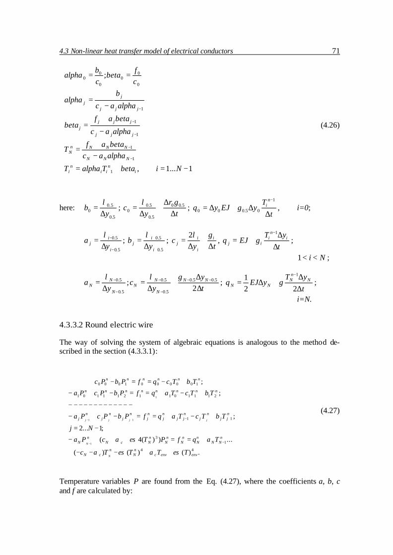
4.3 Non-linear heat transfer model of electrical conductors 71
−=+=
−+
=
−
+=
−=
==
+
−
−
−
−
−
1...1,
;
1
1
1
1
1
1
0
00
0
00
NibetaTalphaT
alphaacbetaaf
T
alphaac
betaafbeta
alphaac
balpha
cf
betacb
alpha
in
iin
i
NNN
NNNnN
jjj
jjjj
jjj
jj
(4.26)
here: 5.0
5.00 y
b∆
=λ
; t
ry
c∆
∆+
∆= 5.00
5.0
5.00
γλ;
tT
yEJyqn
i
∆∆+∆=
−1
05.000 γ , i=0;
5.0
5.0
−
−
∆=
i
ij y
aλ
; 5.0
5.0
+
+
∆=
i
ij y
bλ
; ty
c i
i
ij ∆
+∆
=γλ2
, t
yTEJq i
ni
ij ∆∆
+=−1
γ ;
Ni <<1 ;
5.0
5.0
−
−
∆=
N
NN y
aλ
;ty
yc NN
N
NN ∆
∆+
∆= −−
−
−
25.05.0
5.0
5.0 γλ;
tyT
yEJq Nn
NNN ∆
∆+∆=
−
221 1
γ ;
i=N.
4.3.3.2 Round electric wire
The way of solving the system of algebraic equations is analogous to the method de-scribed in the section (4.3.3.1):
++−−−+
+==+++−
−=
+−+==−+−
−−−−−−−−−−−−−
+−+==−+−
+−==−
−
+−
−
+−
.)()()(
...))(4(
;1...2
;
;
;
44
13
11
2111011211101
1000001000
1
11
1
envenvcnN
ncN
nNN
nN
nN
nN
nNcN
nN
njj
nj
njj
nj
nj
nj
nj
nj
nnnnnnnn
nnnnnn
TTTTc
TaqfPTcPa
Nj
TbTcTaqfPbPcPa
TbTcTaqfPbPcPa
TbTcqfPbPc
N
N
jjjj
εσαεσα
εσα
(4.27)
Temperature variables P are found from the Eq. (4.27), where the coefficients a, b, c and f are calculated by:

72 Chapter 4 Numerical calculation of temperature behaviour in a transient state regime
5.0
5.05.00 r
rb
∆=
λ;
trr
rr
c∆
∆+
∆= 5.05.00
5.0
5.05.00
γλ;
tT
rEJrrqn
i
∆∆+∆=
−1
05.005.00 γ , i=0;
5.0
5.05.0
−
−−
∆=
i
iij r
ra
λ;
5.0
5.05.0
+
++
∆=
i
iij r
rb
λ;
tr
rr
c ii
i
iij ∆
∆+
∆=
γλ2,
tT
rEJrrqn
iiiiij ∆
∆+∆=−1
γ , Ni <<1 ;
rr
a N ∆=
λ;
trr
rr
cN ∆∆
+∆
=2
γλ;
tT
rEJrqn
NNN ∆
+∆=−1
21
γ , i=N.
4.3.3.3 Electric fuse
In order to calculate the temperature distribution in the fuse system a non- linear system of equations has to be solved because of the radiation term in the equation (4.16). We use, as in previous cases a Newton-Raphson method to solve the problem. The system of algebraic equations is given as follows:
=+−
−=
+++−
+−+=−+++−
−−−−−−−−−−−−−+++−
+−+=−+++−
=−
−
+
−+−
.
;1...1
;)()(
)())(4(
;)(
)())(4(
;
11
144
113
1
2144
1
1012113
1101
01000
11
µ
µ
εσαεσ
αεσα
εσαεσ
αεσα
TTcTa
Nj
TbuTuTuT
TucTaqPbPuTucPa
TbuTuTuT
TucTaqPbPuTucPa
TTbTc
nNN
nNN
njjenvenv
nj
nj
njj
nnjj
nj
njj
njj
nenvenv
n
nnnnnnn
nn
jj
(4.28)
Here the coefficients a, b, c and p are calculated as follows:
10 =c ; 10 =b ; 1050 =µT ; i = 0;
5.0
5.05.0
−
−−
∆=
i
iij x
Aa
λ;
5.0
5.05.0
+
++
∆=
i
iij x
Ab
λ;
tx
xA
c ii
i
iij ∆
∆+
∆=
γλ2,
txT
AEJq in
iij ∆
∆+=
−1
γ , i = 1,2,…,N-1;
1=Na ; 1=Nc ; 1051 =µT , i = N. Results of numerical simulation using the approach developed in this chapter together with a validation procedure are presented in Chapter 6. Flat electrical cables of different conductor size supplied by the company Technology & Innovation GmbH and round

4.3 Non-linear heat transfer model of electrical conductors 73 electrical wires supplied by the company Leoni Bordnetze GmbH were used. Fuse ele-ment samples were provided by DaimlerChrysler AG.

________________
CHAPTER 5 ________________
BASIC CONSIDERATIONS OF THE EXPERIMENT AND
EXPERIMENTAL SETUP
This chapter presents the theory of the experimental procedure used in this work to-gether with the measurement setup and the data acquisition. The aim of the experiments was to investigate the electrical load capacities of various electrical wires and cables. For this, two types of measurements were required: a) Current versus voltage measurement, b) Resistance versus temperature measurement The investigation commenced with the measurement of power dissipation as function of temperature of the wire surface, called “current versus voltage measurement”,(a). The next step was to validate the linear temperature coefficient αT, called “resistance versus temperature measurement”,(b). Later the information from both experiments was used to correct the theoretical model, if necessary. First, some information on how properly the measurements have to be performed will be given. The theoretical background for the measurement specification was developed extensively during this research work. Then, a figure detailing the experimental set up for both cases will be shown. The procedure of parameter acquisition using GPIB (Gen-eral Purpose Interface Bus) devices and the appropriate software will be also presented. The programme is given in the Appendix C.
5.1 Basic considerations of the experiment 5.1.1 Resistance versus temperature measurement The aim of this experiment is to determine the linear temperature coefficient αT of cop-per wires and cables. Later, this temperature coefficient αT is used to calculate the wire and cable temperature from the current versus voltage relationship obtained from the second experiment: the current versus voltage measurement. The electrical resistance Ri of the wire has to be determined for different applied tem-perature Ti values of the wire. These temperatures are achieved by heating up the cable in a heat chamber. Chamber temperature Tch should be increased in equal steps from environment temperature Tenv up to max. cable temperature T. In order to avoid errors

76 Chapter 5. Basic considerations of the experiment and experimental setup caused by an unsteady state during the measurement, the resistance of cable should be also measured for decreasing temperature values down to Tenv. During the measurement process, the cable is not heated electrically. For the qualitative measurement, the following three conditions must be fulfilled: a) For every resistance measurement step, temperature steady-state condition must be obtained, b) The measurement error due to material restraints must be estimated, c) Thermo voltages must be avoided. A. Requirements for a steady-state temperature condition Here, the most important parameter is a steady-state time t, after which temperature dif-ference between Tch and cable temperature T0 becomes zero. The time t is influenced by a time constant τ , which is different for every wire type. In order to calculate steady-state time t, one should determine the factor n, i.e. the number of time constants τ needed to reach a steady-state: τnt = (5.1) To calculate factor n, we can consider the precision of the heating chamber temperature. We can assume that the temperature difference δTL between the cable temperature and chamber temperature should be equal to the temperature error of the chamber δTch: ch
nL TTeT δϑδ == − (5.2)
From there, the factor n is given by:
chTT
nδϑ
ln= (5.3)
where: δTL temperature difference between cable and chamber temperatures in K δTch temperature measurement error of the heating chamber in K
τ thermal time constant of the cable in s ϑT step size of temperature interval in K n time constant factor t steady-state time in s
Here we consider δTch from the technical specification of heating chamber 0.5 K. Step size of temperature interval for resistance measurement is ϑT = 10 K. Then, the n factor is calculated: 3996.25.0/10ln ≈=≥n
(5.4)

5.1 Basic considerations of the experiment 77
this means, that only after 3τ cable resistance can be measured. B. Permissible measurement error of cable resistance. In order to estimate permissible measurement error of cable resistance, we ought to use the following formula:
[ ] [ ]20
2000 )()(1)()(1)( TTRTTTTRtR TTTT ∆+∆+=−+−+= βαβα (5.5)
After differentiation, we obtain:
[ ] TdTRtdR TT ∆∆+= βα 2)( 0 (5.6) For ßT = 0, equation (5.6) simplifies to:
TRdTdR
α0= (5.7)
If we apply a small difference to the resistance δR and temperature δT, we get a tem-perature error based on reference resistance R0(T0) at reference temperature T0 :
TR
RRRR
Tδαδ
=−
=0
12
0
(5.8)
In the case that measurement error of temperature does not exceed a value of
5.0<Tδ K, we get maximal permissible relative resistance error δR/R0 for copper:
%2.0%19.00
≈≤=≤RRδ
(5.9)
The total measurement error consists of measured cable temperatures δTc1 (heating up), δTc2 (cooling down) and error of heating chamber temperature δTch: δT = δTc1+ δTc2 + δTch (5.10) Inserted in the equation (5.8) we obtain the following maximal allowed resistance error:
- linear part: TT T αβ <<∆2

78 Chapter 5. Basic considerations of the experiment and experimental setup
chT TRR
δαδ
30
= (5.11)
- linear and square part:
chTT TTRR
δβαδ
)2(30
∆+= (5.12)
here: 0RRδ
- maximal permissible resistance error.
For the temperature interva l ∆T=0 to 120K (or considering environment temperature Tenv= 20°C, T=20 to 140°C) we get:
( ) chTRR
δδ
%19.1...14.10
≤≤= (5.13)
Considering the temperature error of the chamber δTch ≤ 0.5K we obtain maximal
permissible resistance error0RRδ
:
( ) %6.0%60.0...57.00
≈≤≤=RRδ
(5.14)
C. Measurement error due to thermo voltages. Thermo voltages occur if two different metals at different temperatures come into con-tact. It is critical to perform the experiment by measuring voltage drop on the cable rather than doing a four-pole resistance measurement. This is obvious from the follow-ing example: Thermo voltage for Cu vs Cu-Fe contact is about 5 µV/K whereas for 100 K it makes 0.5 mV. In case of 4-pole resistance measurement for 1 mm2 copper wire thermo volt-age is: at 1 mA current – only 17.5 µV/m, for 3 m wire - ≈ 50 µV Experiment results are presented in the table 5.1. Here are evaluated linear and square temperature coefficients α65 and ß65 at 65°C reference temperature respectively.
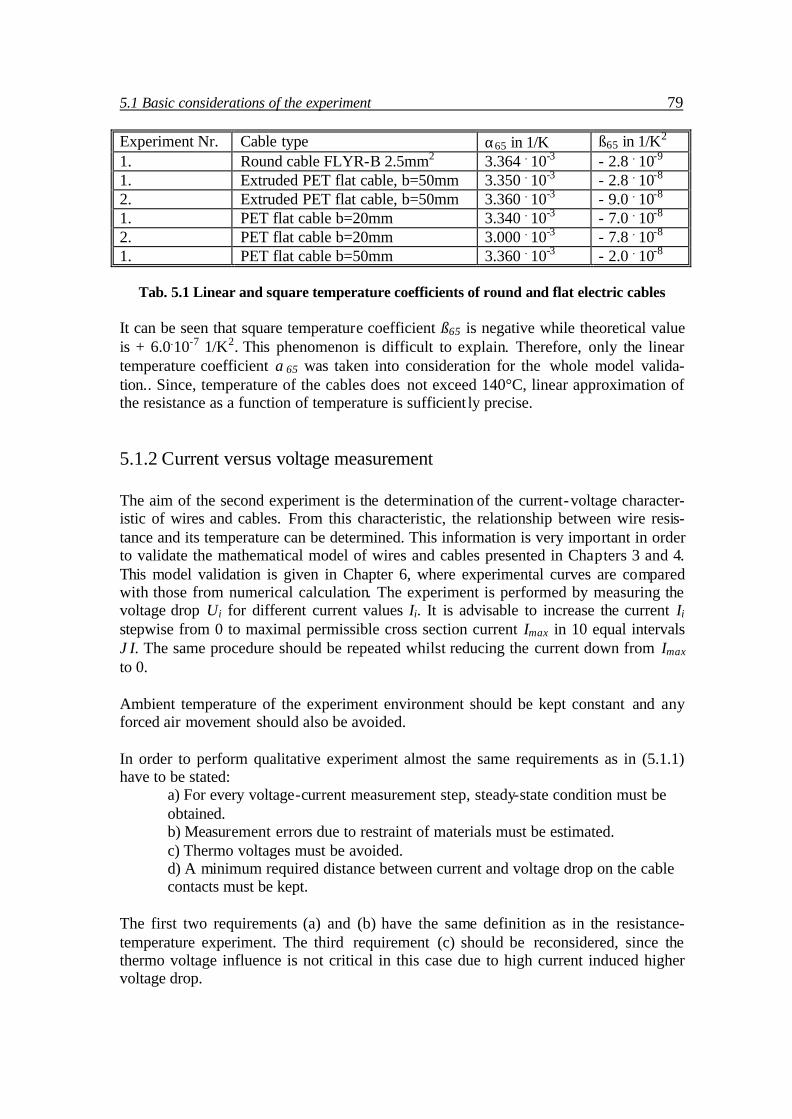
5.1 Basic considerations of the experiment 79
Experiment Nr. Cable type α65 in 1/K ß65 in 1/K2
1. Round cable FLYR-B 2.5mm2 3.364 . 10-3 - 2.8 . 10-9 1. Extruded PET flat cable, b=50mm 3.350 . 10-3 - 2.8 . 10-8
2. Extruded PET flat cable, b=50mm 3.360 . 10-3 - 9.0 . 10-8 1. PET flat cable b=20mm 3.340 . 10-3 - 7.0 . 10-8 2. PET flat cable b=20mm 3.000 . 10-3 - 7.8 . 10-8 1. PET flat cable b=50mm 3.360 . 10-3 - 2.0 . 10-8
Tab. 5.1 Linear and square temperature coefficients of round and flat electric cables
It can be seen that square temperature coefficient ß65 is negative while theoretical value is + 6.0.10-7 1/K2. This phenomenon is difficult to explain. Therefore, only the linear temperature coefficient α65 was taken into consideration for the whole model valida-tion.. Since, temperature of the cables does not exceed 140°C, linear approximation of the resistance as a function of temperature is sufficient ly precise. 5.1.2 Current versus voltage measurement The aim of the second experiment is the determination of the current-voltage character-istic of wires and cables. From this characteristic, the relationship between wire resis-tance and its temperature can be determined. This information is very important in order to validate the mathematical model of wires and cables presented in Chapters 3 and 4. This model validation is given in Chapter 6, where experimental curves are compared with those from numerical calculation. The experiment is performed by measuring the voltage drop Ui for different current values Ii. It is advisable to increase the current Ii stepwise from 0 to maximal permissible cross section current Imax in 10 equal intervals ϑI. The same procedure should be repeated whilst reducing the current down from Imax to 0. Ambient temperature of the experiment environment should be kept constant and any forced air movement should also be avoided. In order to perform qualitative experiment almost the same requirements as in (5.1.1) have to be stated: a) For every voltage-current measurement step, steady-state condition must be obtained. b) Measurement errors due to restraint of materials must be estimated. c) Thermo voltages must be avoided. d) A minimum required distance between current and voltage drop on the cable contacts must be kept. The first two requirements (a) and (b) have the same definition as in the resistance-temperature experiment. The third requirement (c) should be reconsidered, since the thermo voltage influence is not critical in this case due to high current induced higher voltage drop.

80 Chapter 5. Basic considerations of the experiment and experimental setup The thermo voltage for Cu vs. Cu-Fe pair is 5 µV/K, that is for 100 K – 0.5 mV. Con-sidering the voltage drop in 1 mm2 copper wire: For 10 A measurement current, the voltage drop leads to 0.175 V/m. For a 10 m length copper wire (which is a minimum requirement to avoid the influence of the boundary temperature decay) the voltage drop results in 1.75 V. This is about 300 times bigger value as the thermo voltage for 100 K. From this explanation follows that thermo voltages do not significantly influence to measurement error. The distance between current and voltage measurement contacts of non- insulated wire can be calculated according to equations (3.51, Chapter 3) is given by:
02
2
ρααλ
χρ IuA
A−
= (5.15)
Denoting 4
2dA
π= and u=πd we obtain:
02
0232
2
442 ρααλ
ρααπλπ
χρρ dId
Idd
−=
−= (5.16)
We can rewrite equation (5.16) in the following form:
−
=
320
2
121
d
Id
απ
ραα
λχ
ρ
(5.17)
For a small current density, the Eq. (5.17) can be simplified as follows:
αλ
χd
21
= , αλ
χdn
n2
= (5.18)
here: n is the number of length constants, which may be applied ranging from any given temperature to the cable temperature of an infinite length with an acceptable error. For application in this study a factor n = 3, leading to an error of 5 %, is sufficiently precise:
αα
λχ mmdd /897.0
23
3 == (5.19)
here: d cable diameter in mm.

5.1 Basic considerations of the experiment 81
If we consider a critical heat convection coefficient α = 16 and wire diameter of 1.0 mm we get: 3χ = 224 mm ≈ 22 cm Following equations are used to compute cable temperature T as a function of current I: 1. Determination of cable temperature T:
[ ] [ ]2000
200000 )()(1)()(1)( TTRTTTTRTR ∆∆ βαβα ++=−+−+= (5.20)
here: 0α linear temperature coefficient of copper at reference temperature T0 in 1/K 0β square temperature coefficient of copper at reference temperature T0 in 1/K2
Material constants 0α and 0β have been determined by the experiment described in (5.1.1), however only linear temperature coefficients will be used to calculate cable temperature. Cable temperature T is found from Eq. (5.15):
000
11
TRR
T ii +
−=
α
(5.21) here: i number of measurements within one experiment 2. Determination of cable resistance Ri: From voltage drop measurement on the cable at current Ii according to Ohm’s law the resistance is:
i
ii I
UR =
(5.22) here: Ii current calculated by voltage drop on the shunt Usi with constant resitance Rs:
s
sii R
UI =
(5.23)

82 Chapter 5. Basic considerations of the experiment and experimental setup
5.2 Experimental setup 5.2.1 Determination of the cable conductor temperature coefficient Figure 5.1 shows experimental setup for cable resistance / temperature measurement. The cable is placed in a liquid silicon bath, which is situated in a heating chamber (Type: Nixon 815, ISOTECH). The liquid was used as a heat transferring media in or-der to ensure very constant and homogeneous temperature in the cable. The heat cham-ber has its own temperature control, which however is not precise enough for this kind of experiment. Therefore, an additional Pt10 sensor was used to measure the liquid and cable temperature.
High precision digitalmultimeter-miliommeter
Pt10
Liquid silicon
Heatchamber
peristaltic pump
Liquidsilicon bath
Flat/round cable
4-pole resistancemeasurement
GPIB (General Purpose Interface Bus)
GPIB
Fig. 5.1 Experimental setup for the cable conductor resistance measurement at different
temperatures for the determination of the temperature coefficient The voltage and the current measurement connection wires were soldered to the cable and sealed with temperature resistant insulating epoxy adhesive. This insulation is very important in order to avoid short circuits in the fluid. Resistance measurement was per-formed by the 81/2 digits precision digital multimeter PREMA 6040S. This multimeter as well as the heat chamber was controlled by a GPIB (General Purpose Interface Bus) controller, which allows the automation of the whole experiment. The liquid silicon is circulated by a pump, which allows more precise temperature control. All input data
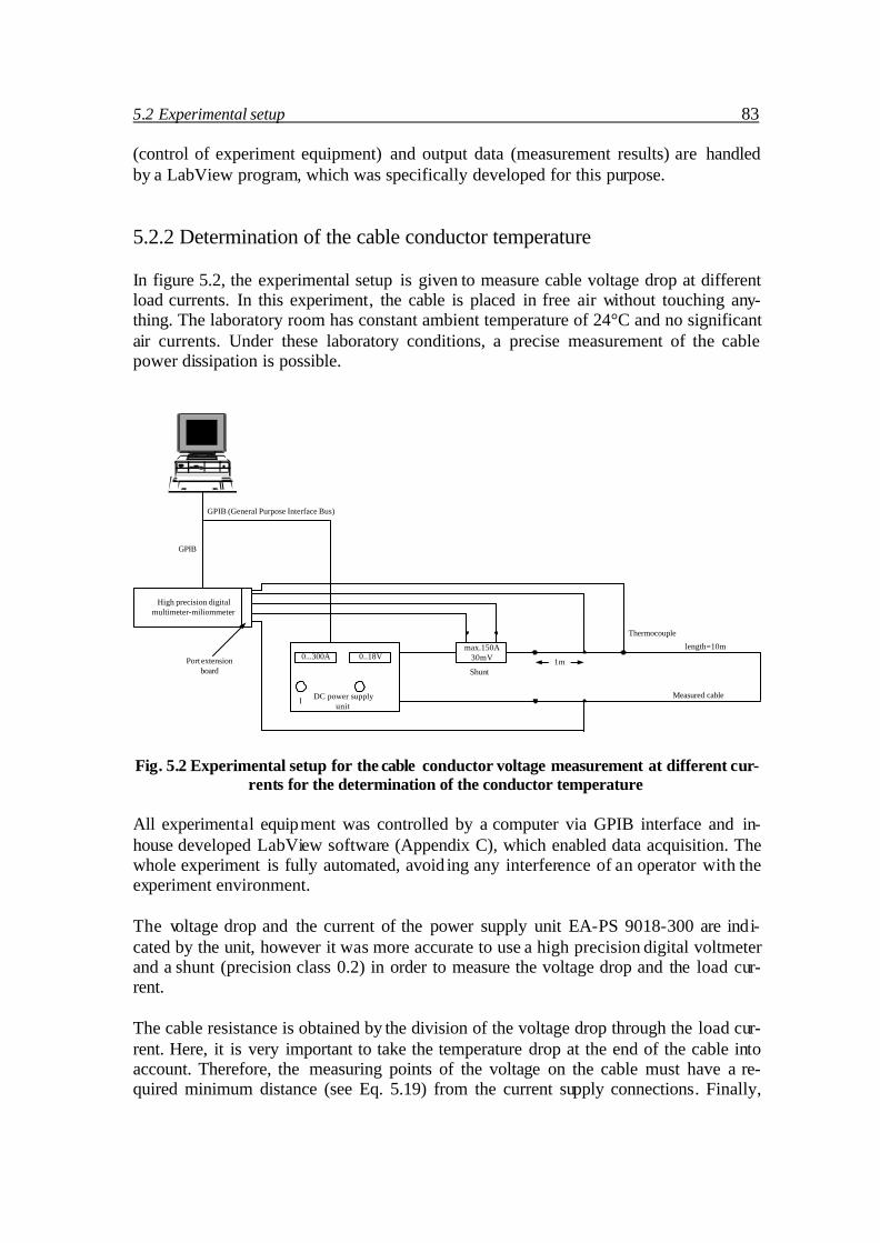
5.2 Experimental setup 83
(control of experiment equipment) and output data (measurement results) are handled by a LabView program, which was specifically developed for this purpose. 5.2.2 Determination of the cable conductor temperature In figure 5.2, the experimental setup is given to measure cable voltage drop at different load currents. In this experiment, the cable is placed in free air without touching any-thing. The laboratory room has constant ambient temperature of 24°C and no significant air currents. Under these laboratory conditions, a precise measurement of the cable power dissipation is possible.
High precision digitalmultimeter-miliommeter
GPIB
max.150A30mV0...300A 0..18V
I
length=10m
Port extensionboard
1m
Measured cableDC power supplyunit
Shunt
Thermocouple
GPIB (General Purpose Interface Bus)
Fig. 5.2 Experimental setup for the cable conductor voltage measurement at different cur-
rents for the determination of the conductor temperature All experimental equipment was controlled by a computer via GPIB interface and in-house developed LabView software (Appendix C), which enabled data acquisition. The whole experiment is fully automated, avoid ing any interference of an operator with the experiment environment. The voltage drop and the current of the power supply unit EA-PS 9018-300 are indi-cated by the unit, however it was more accurate to use a high precision digital voltmeter and a shunt (precision class 0.2) in order to measure the voltage drop and the load cur-rent. The cable resistance is obtained by the division of the voltage drop through the load cur-rent. Here, it is very important to take the temperature drop at the end of the cable into account. Therefore, the measuring points of the voltage on the cable must have a re-quired minimum distance (see Eq. 5.19) from the current supply connections. Finally,

84 Chapter 5. Basic considerations of the experiment and experimental setup the cable temperature is calculated from the cable resistance with the help of the con-ductor temperature coefficient. For the sake of redundancy, a second independent method to receive cable temperature has been applied by using a nickel-constantan thermocouple sensor, which was attached to the cable surface. This sensor was also used for safety to cut off the power supply unit if the maximum allowed temperature of the cable is exceeded. Thermocouple sensors measure very precisely even if only very small surfaces are available. This is very important for small size electric cables. It would not be possible to measure the temperature of such cables with a Pt100 sensor. The disadvantage of thermocouples is however, that a very precise reference temperature of zero degrees is required. For this purpose, a water- ice mixture was used. 5.3 Measuring process and parameter acquisition 5.3.1 Determination of the cable conductor temperature coefficient The measuring algorithm of the resistance vs. temperature characteristic of the cable is given in by P. Mack [24]. During this measuring process the cable resistance was meas-ured by 4-pole measurement and its results saved in the computer. Temperature of the cable was measured by Pt10 sensor, which had been placed as close as possible to the cable. The resistance of Pt10 was also measured by the same digital multimeter (DMM) and later, resistance values were converted to the temperature. This conversion is possi-ble by the empirical equation:
−
°
−
°
−
°°+= 1
74.6301
58.4191
100100045.0
'''''
CT
CT
CT
CT
TT (5.19)
here T’ is given by the equation:
[ ]
−
°°+−= 1
1001001)(
1 '''
CT
CT
TWT δα
(5.20)
or,
100002
1)(10000
4100
1100
12
'
δα
δδδ −−
+−−
+
=
TW
T (5.21)
5.3 Measuring process and parameter acquisition 85
here: )0(/)()( CRTRTW °= , R(T) measured resistance of Pt10 sensor in Ω, R(0°C) = 10.62796 in Ωm, α = 3.925870.10-3 in 1/K, δ = 1.496225 in °C. 5.3.2 Determination of the cable conductor temperature The measuring process and data acquisition of the voltage vs. current experiment had been implemented in Pascal language by T. Roida [25] and later improved in LabView by the author of this study (see also Fig. 5.3, 5.4). The idea of the measuring process is illustrated in the following table: Set the power supply unit to 15 VDC The user defines the step size and interval of currents from i = 1 to n + 1
(n = number of currents) The user sets the number of measurements for a single current value from i = 1 to m (m = number of measurements of one current value)
The user sets one waiting time for all the measurements in s
Steady state = Number of measurement times (Waiting time for one measurement ) Reset the power supply to 0 A Close the files
Tab 5.1 Algorithm of the measurement program
The visualisation of the measurement data is given in the figures 5.5 and 5.6. The time scale (Fig. 5.5) illustrates the measurement procedure and gives information about the transient state regime. In Fig. 5.6 the temperature of an insulated copper wire is depicted as function of the load current.

86 Chapter 5. Basic considerations of the experiment and experimental setup
Fig. 5.3 Experimental setup of flat electric cable (FFC)
Fig. 5.4 Experimental setup of round electric cable
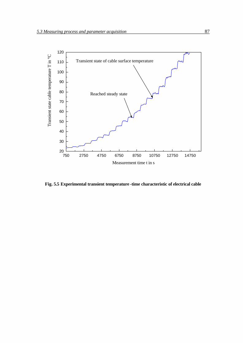
5.3 Measuring process and parameter acquisition 87
750 2750 4750 6750 8750 10750 12750 1475020
30
40
50
60
70
80
90
100
110
120
Reached steady state
Transient state of cable surface temperature
Tran
sien
t sta
te c
able
tem
pera
ture
T in
°C
Measurement time t in s
Fig. 5.5 Experimental transient temperature -time characteristic of electrical cable

88 Chapter 5. Basic considerations of the experiment and experimental setup
20 40 60 80 100 120 140 160 180 20020
30
40
50
60
70
80
90
100
110
120
Mea
sure
d st
eady
sta
te c
able
tem
pera
ture
T in
°C
Measurement current I in A
Fig. 5.6 Experimental steady-state temperature -current characteristic of electrical cable
________________
CHAPTER 6 ________________
MATHEMATICAL MODEL
VALIDATION AND INTERPOLATION OF
THE NUMERICAL RESULTS
This chapter starts with the validation of the numerical simulation by the measurement results. Section 6.2 presents a least-square interpolation of the validated results. The theoretical model is determined by the thermal conductivity of insulating materials, the temperature coefficient of copper resistance and the convection and radiation coeffi-cients. The numerical results are fitted by polynomial or logarithmic functions, where the coefficients of those functions are obtained by applying the least-square technique.
6.1 Mathematical model validation Before starting the comparison of the theoretical (numerical) results with the experi-mental ones, the quality of the model equations and the evaluation procedure for fitting them to the experimental data should be checked. The quality of derived heat equations can be understood as the reduction of a 3-D model to a 1-D model. During experimental work, the model reduction to 1-D problem turned out to be sufficient with a negligible error between the theoretical and the physical model. In addition, boundary conditions can be considered as the quality factor. Implemented limit conditions must be as close to realistic conditions as possible. In our model, the boundary conditions represent laminar free convection to the air while the effects caused by turbulent convection were neglected. In reality, the experiments were per-formed in an environment where the forced convection was minimised. In addition, convection caused by turbulence was negligible. The first step was to the validate linear temperature coefficient of the conductor resis-tance αρ, since this parameter is important for the conductor electrical resistance behav-iour in the theoretical model. The basic material for the production of stranded conduc-tors for automotive wires is oxygenic copper according to DIN 40500, part 4. The DIN designation of this conductor type is E-CU 58 F21. Since this material does not consist of pure copper, and the manufacturing process might have changed the properties, it

90 Chapter 6. Mathematical model validation and interpolation of the numerical results was necessary to measure and validate temperature coefficient of copper resistance again. Below the measurement results of conductor resistance as a function of temperature are given:
0 20 40 60 80 100
0.072
0.078
0.084
0.090
0.096
0.102
0.108
R =0.07523[1+0.004dT]
Res
ista
nce
R in
om
s
Temperature deltaT in K
Measurement data Polynomial fit of measurement data.
Reference temperature - 20°C
Fig. 6.1 Measured resistance R of round wire for temperature range from 0 to 100 K.
Measured temperature coefficient of copper resistance is αρ = 0.004 1/K (based on 20 °C)
0 10 20 30 40 50 60
0.088
0.092
0.096
0.100
0.104
0.108
Measurement data Polynomial fit of measurement data.
Reference temperature - 65°C
R =0.088711[1+0.00336dT]
Res
ista
nce
R in
om
s
Temperature deltaT in K
Fig. 6.2 Measured resistance R of round wire for a temperature range from 0 to 60 K.
Measured temperature coefficient of copper resistance is αρ = 0.0036 1/K (based on 65 °C)

6.1. Mathematical model validation 91 From the measurement results (Fig.6.1) it can be seen that αρ has a value of 0.004 1/K instead of 0.0038 1/K as given in the literature for pure copper material. Figure 6.2 shows a temperature coefficient of 0.0036 1/K (based on 65 °C), which cor-responds the value of 0.004 1/K (based on 20 °C). The value of 0.0036 1/K is also use-ful, since all our calculations are based on the environment temperature of 65°C. Below are equations for the conversion of the temperature coefficient αρ to any refer-ence temperature. For the derivation, the following functions of the electrical resistance R(T) through the points T1 and T2 are considered:
( )( )
∆+∆+=
∆+∆+=2
21222
211111
1)(
1)(
TTRTR
TTRTR
βα
βα (6.1)
here: nn TTT −=∆ The aim is to obtain a relationship between α2 and α1. First and second order derivatives of Eq. (6.1) are:
( )1111' 2)( TRTR ∆+= βα (6.1a)
( )2222
' 2)( TRTR ∆+= βα (6.1b)
11'' 2)( RTR β= (6.1c)
22'' 2)( RTR β= (6.1d)
1122 RR ββ = (6.1e)
)(2 12111122 TTRRR −+= βαα (6.1f)
2
1211121112 )()( TTRTTRRR −+−+= βα (6.1g) Then the result is the following:
( ) ( )[ ]212112112 1 TTTTRR −+−+= βα (6.2)
( )
( ) ( )2121121
12112
1
2
TTTT
TT
−+−+
−+=
βα
βαα (6.3)
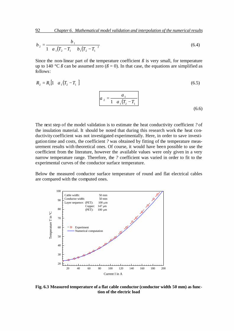
92 Chapter 6. Mathematical model validation and interpolation of the numerical results
( ) ( )2121121
12
1 TTTT −+−+=
βα
ββ (6.4)
Since the non- linear part of the temperature coefficient ß is very small, for temperature up to 140 °C ß can be assumed zero (ß = 0). In that case, the equations are simplified as follows:
( )[ ]12112 1 TTRR −+= α (6.5)
( )121
12 1 TT −+
=α
αα
(6.6) The next step of the model validation is to estimate the heat conductivity coefficient ? of the insulation material. It should be noted that during this research work the heat con-ductivity coefficient was not investigated experimentally. Here, in order to save investi-gation time and costs, the coefficient ? was obtained by fitting of the temperature meas-urement results with theoretical ones. Of course, it would have been possible to use the coefficient from the literature, however the available values were only given in a very narrow temperature range. Therefore, the ? coefficient was varied in order to fit to the experimental curves of the conductor surface temperature. Below the measured conductor surface temperature of round and flat electrical cables are compared with the computed ones.
20 40 60 80 100 120 140 160 180 200
20
30
40
50
60
70
80
90
100Cable width: 50 mmConductor width: 50 mmLayer sequence: (PET): 100 µm Copper: 147 µm (PET): 100 µm
Tem
pera
ture
T in
°C
Current I in A
Experiment Numerical computation
Fig. 6.3 Measured temperature of a flat cable conductor (conductor width 50 mm) as func-
tion of the electric load

6.1. Mathematical model validation 93
20 40 60 80 100 120 140 160 180 200 220 240 260
20
30
40
50
60
70
80
90
100Cable width: 74 mmConductor width: 74 mmLayer sequence: (PET): 100 µm Copper: 162 µm (PET): 100 µm
Tem
pera
ture
T in
°C
Current I in A
Experiment Numerical computation
Fig.6. 4 Measured temperature of a flat cable conductor (conductor width 74 mm) as
function of the electric load
Fig. 6. 5 Flat cable (FFC) examples

94 Chapter 6. Mathematical model validation and interpolation of the numerical results
2 4 6 8 10 12 14 16 18
30
40
50
60
70
80
90
100
110
120Conductor cross-section: 0.5 mm2
Conductor: copper Cu58 F21Insulation: (PE)
Tem
pera
ture
T in
°C
Current I in A
Experiment Numerical computation (lambda=0.58) Numerical computation (lambda=0.4)
Fig. 6. 6 Measured temperature of a round wire conductor (cross section 0.5mm2) as func-
tion of the electric load
20 40 60 80 100 120 140 160 180 200 220 240
20
30
40
50
60
70
80
90
100Conductor cross-section: 35 mm2
Conductor: copper Cu58 F21Insulation: (PVC)
Tem
pera
ture
T in
°C
Current I in A
Experiment Numerical computation
Fig. 6. 7 Measured temperature of a round wire conductor (cross section 35mm2) as func-
tion of the electric load

6.1. Mathematical model validation 95
Fig. 6. 8 Round cable examples
0,0 0,2 0,4 0,6 0,8 1,020
40
60
80
100
120
140
160
180
40 Amp60 Amp
80 Amp
100 Amp
120 Amp
140 Amp
160 Amp
180 Amp
Length in m
Tem
pera
ture
T in
°C
Experiment Numerical computation
Fig. 6.9 Measured temperature of a fuse element as function of the electric load

96 Chapter 6. Mathematical model validation and interpolation of the numerical results
Fig. 6.10 Fuse element prototype with temperature sensors (thermocouples). Fuse element (hollow cylinder) dimensions: inner diameter – 6mm, outer diameter 8mm. Material type
of the fuse element: Bras 58 (CuZn39Pb3). Finally, the heat convective and radiative coefficients had to be validated. During sepa-rate experimental work [18] a number of measurements of various round wires was car-ried out in order to validate the empirical heat convection and radiation formulas, which were presented in the section (2.5). The results of this experimental work have shown that the evaluation procedure of convection and radiation coefficients is correct. Since, it has already been described how the model was validated, now the obtained re-sults can be studied. The following three models, which differ by the geometry and type of materials are presented: 1. Figures 6.3 and 6.4 show the flat cable conductor temperature as function of the elec-trical current. These results are obtained for a cable, which is placed free in air, in a horizontal position. The temperature is taken after the steady state has been reached. Both, numerical simulation and measurement data, gives a very good agreement. 2. Figures 6.6 and 6.7 show the round wire conductor temperature as function of the electrical current. By altering of the conductivity coefficient λ of PE (Polyethylene) in figure 6.6, a better agreement of both curves can be achieved. 3. Figure 6.9 shows the temperature distribution along the fuse element. The length of the whole system was about 1 meter, since the influence of the fuse holders and contacts must be considered. Also electrical wire, which is protected by this fuse had to be taken into consideration too. The temperature distribution is presented for different electrical current values. The calculated curves in all figures match with the measured data ac

6.2. Interpolation of the numerical results to reduce heat transfer equations 97 ceptably well. At the boundaries of the fuse holders and contacts, a larger error is pre-sent. This can be explained by the limited performance of the experiment setup. Tem-perature of the fuse system was measured only by three thermocouple sensors.Later, three measurement points were interpolated. However, high accuracy of tempera-ture gradient on the boundaries is not of primary importance. Only the fuse element maximal temperature is of interest, because this temperature causes the required inter-ruption of the fuse-melting element. Discussed results show the fact that the approximation made for the derivatives of the equations (Chapter 2: 2.4, 2.6, 2.8) as well as the validation of the physical model con-stants are applicable under the experimental conditions, which are interested in this con-text.
6.2 Interpolation of the numerical results to reduce heat transfer equations
Throughout the entire study, the heat transfer analysis algorithm was derived using ana-lytical / numerical methods. This algorithm allows the determination of the thermo-electrical characteristic of electrical conductors in both a steady- and transient-state re-gimes. The proposed approach provides very good accuracy between theory and ex-perimental results, is applicable for different conductor geometries, and can be extended from a 1-D to a 2-D problem. However, very often, numerical simulation of heat trans-fer requires a lot of computation time that is not acceptable if the numerical simulation routine has to be integrated into another complex simulation system. This leads finally to a situation, where the whole performance of a complex simulation system becomes very poor. Another disadvantage of pure numerical simulation of heat transfer problem is that very often in a real life, the calculations have to be done very quickly and in a simple manner Therefore, our intension in this study is not only to present fully-developed numerical models but also to develop simple, with the minimum number of physical constants, analytical equations, which describe best the steady-state and transient-state heat trans-fer regimes in any type of conductors. These equations should have the advantage of producing a manageable relationship having only two or three constants, which can be obtained easily by the least-square (LS) algorithm. Finally, having those simple equa-tions, an operator can perform the calculations in an easy way. In this section we will present polynomial and logarithmical equations of thermo-electrical characteristics and show how to apply the LS algorithm [8,9] for the calcula-tion of the “simplified-equation” coefficients. It is very important to predict correctly the correct equations with a minimum number of unknown constants. Basically, two type of functions are of interest: polynomial regression and logarithmical functions. With these two functions, all important thermo-electrical characteristics can be de-scribed. The following functions are considered, whose physical meaning will be given later:
- thermo-electrical characteristic ∆T(I) (Fig.6.11)
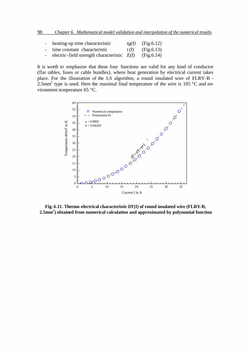
98 Chapter 6. Mathematical model validation and interpolation of the numerical results
- heating-up time characteristic tg(I) (Fig.6.12) - time constant characteristic τ(I) (Fig.6.13) - electric- field strength characteristic E(I) (Fig.6.14)
It is worth to emphasise that these four functions are valid for any kind of conductor (flat cables, fuses or cable bundles), where heat generation by electrical current takes place. For the illustration of the LS algorithm, a round insulated wire of FLRY-B - 2.5mm2 type is used. Here the maximal final temperature of the wire is 105 °C and en-vironment temperature 65 °C.
0 5 10 15 20 25 30 350
5
10
15
20
25
30
35
40
45
50
55
60
a = 0.0802b = 0.04269
dT = a
*I + b*
I2
Tem
pera
ture
del
taT
in K
Current I in A
Numerical computation Polynomial fit
Fig. 6.11. Thermo-electrical characteristic ∆T(I) of round insulated wire (FLRY-B,
2.5mm2) obtained from numerical calculation and approximated by polynomial function

6.2. Interpolation of the numerical results to reduce heat transfer equations 99
20 40 60 80 100 120 140
0
50
100
150
200
250
300
I0
tau = 79.55685I0 = 29.7
Hea
ting
up ti
me
tg in
sec
Current I in A
Numerical computation Logarithmical fit
Fig. 6.12. Heating-up time tg(I) characteristic of round insulated wire (FLRY-B, 2.5mm2)
obtained from numerical calculation and approximated by logarithmical function
0 10 20 30 40 50 60 70 80
75
80
85
90
95
100
105
110
tau0 = 106.2978
c = 7.124d = 0.00935
tau = tau0 - c* I0.5+ d*I2
Tim
e co
nsta
nt ta
u in
sec
Current I in A
Numerical computation Polynomial fit
Fig. 6.13. Time constant τ(I) characteristic of round insulated wire (FLRY-B, 2.5mm2) ob-
tained from numerical calculation and approximated by polynomial function

100 Chapter 6. Mathematical model validation and interpolation of the numerical results
3 6 9 12 15 18 21 24 27 300.02
0.04
0.06
0.08
0.10
0.12
0.14
0.16
0.18
0.20
0.22
0.24
0.26
0.28
0.30
Elec
trica
l mFi
eld
Stre
nght
E in
V/m
Current I in A
Fig. 6.14 Electric field strength E(I) characteristic of round insulated wire (FLRY-B,
2.5mm2) obtained from Eq. (6.10)
The curves presented in figures 6.11, 6.12, 6.13 and 6.14 can be described by the fo l-lowing equations: - thermo-electrical characteristic (here 0≥I ):
( ) 20 IbIaIIT +=≤∆
(6.7) - heating-up time characteristic:
( ) 20
2
2
0 lnII
IIIt gg −
=> τ
(6.8) - time constant characteristic:
25.00 IdIc +−= ττ
(6.9) - electrical field strength characteristic:
A
TTI
AI
E))(1( 2
0 ∆+∆+== ρρ βαρρ
(6.10)
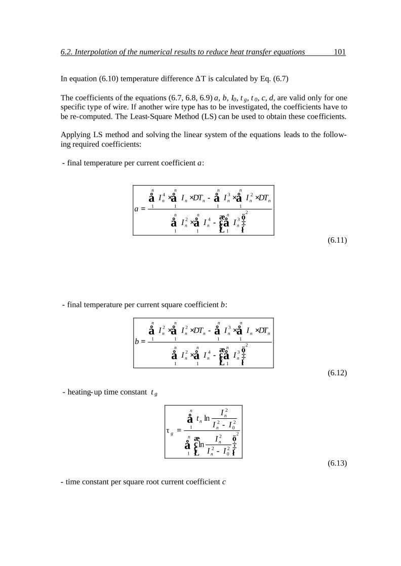
6.2. Interpolation of the numerical results to reduce heat transfer equations 101 In equation (6.10) temperature difference ∆T is calculated by Eq. (6.7) The coefficients of the equations (6.7, 6.8, 6.9) a, b, I0, τg, τ0, c, d, are valid only for one specific type of wire. If another wire type has to be investigated, the coefficients have to be re-computed. The Least-Square Method (LS) can be used to obtain these coefficients. Applying LS method and solving the linear system of the equations leads to the follow-ing required coefficients: - final temperature per current coefficient a:
2
1
3
1
4
1
2
1 1 1 1
234
−⋅
⋅⋅−⋅⋅=
∑∑∑
∑ ∑ ∑ ∑n
n
n
n
n
n
n n n n
nnnnnn
III
TIITIIa
∆∆
(6.11) - final temperature per current square coefficient b:
2
1
3
1
4
1
2
1 1 1 1
322
−⋅
⋅⋅−⋅⋅=
∑∑∑
∑ ∑ ∑ ∑n
n
n
n
n
n
n n n n
nnnnnn
III
TIITIIb
∆∆
(6.12) - heating-up time constant τg
∑
∑
−
−=
n
n
n
n
n
nn
g
III
III
t
1
2
20
2
2
120
2
2
ln
lnτ
(6.13) - time constant per square root current coefficient c

102 Chapter 6. Mathematical model validation and interpolation of the numerical results
2
1
5.2
1
4
1
1 1 1 1 1 1
25.2
1 1
5.025.220
25.00
−⋅
⋅+⋅−⋅−⋅=
∑∑∑
∑ ∑ ∑ ∑ ∑ ∑∑ ∑n
n
n
n
n
n
n n n n n n
nnn
n n
nnnnnnn
III
IIIIIIIIc
ττττ
(6.14) - time constant per square current coefficient d
∑∑∑
∑ ∑ ∑ ∑ ∑ ∑∑ ∑
⋅−
⋅+⋅−⋅−⋅=
=
n
n
n
n
n
nn
n n n n n n
nnn
n n
nnnnnn
III
IIIIIIIId
1
4
1
2
1
5.2
1 1 1 1 1 1
5.05.2
1 1
25.05.20
20 ττττ
(6.15) here: n,1=∀ ; where n is the number of calculating points in the wire characteristics; In – the electrical current values, which are used in the characteristics of Fig. 6.11-6.14 ∆T – temperature values, which are used in the characteristic of Fig. 6.11 tn – heating up time values, which are used in the characteristic of Fig. 6.12 τn – time constant values, which are used in the characteristic of Fig. 6.13 The relationship presented in Fig. 6.11 is a steady-state load characteristic of electric cables. Here the temperature represents the steady-state for a particular load current value. Normally, this characteristic ends with the maximum allowed temperature of the wire or cable after infinite time. In Fig. 6.12 heating up time is given as a function of the load current. This relationship is well known from the fuse time-current characteristic and it makes sense to apply the same characteristic to any electric wire or cable. The heating up time is the time to reach maximal permissible temperature with a current greater than the nominal load. For example, in Fig. 6.12 105 °C degrees are given as maximal permissible temperature. Having available the time-current characteristics for both: wires and fuses, it is possible to model the geometry of the fuse to match the heat-ing-up time function of the wire. Finally, having a fuse with such a characteristic, it is possible to protect the wire with good accuracy. Fig. 6.13 gives the time constant as a function of load current. This curve gives the pos-sibility to obtain any τ constant as a function of only one variable; the current. It is also straightforward to compute the transient state analytically, having τ as the known pa-rameter. Fig. 6.14 represents the electric field strength dependence on load current. Here, the non- linear curve behaviour is due to non-linear electric resistance dependence on tem-perature.

________________
CHAPTER 7 ________________
CALCULATION OF THE HEAT TRANSFER IN A
MULTI-WIRE BUNDLE Contrary to previous chapters, where the heat transfer was modelled for a single electric cable, in this chapter possible methods to calculate the heat conduction in a multi-cable bundle will be shown. The main effort to solve this problem is devoted to the linear co-ordinate transformation in order to simplify the model geometry and to the determina-tion of an averaged heat conductivity coefficient of the multi-cable material media. This chapter deals with a one-dimensional radial steady state heat conduction problem, where the heat transfer equation is solved analytically. In analogy to a single insulated conductor (see Fig. 7.1a), the multi- insulated cable conductor (see Fig. 7.1b) is consid-ered as an insulated “mixed” conductor. 7.1 Coordinate transformation of the multi-wire bundle geometry The calculation of heat transfer in a multi-cable bundle belongs to the heat conduction problems for anisotropic multi- layered media [28]. The heat conductivity coefficient has been determined using conservative averaging method for layered media [78], where heat conductivity of single cables are transformed to a common mixed property or mixed heat conductivity coefficient. The algorithm of temperature determination using a conservative averaging method can be found in Chapter 8, (3) The calculation method considers an anisotropic material that is homogeneous and has constant thermo-physical properties. It also considers radial symmetry, i.e. no angular temperature gradient φ∂∂ /T = 0. Then, the governing partial differential equation for the heat conduction problem in a cylindrical coordinate system becomes:
)()(1
rqrrT
rrr V=
∂∂
∂∂
− λ (7.1)
here: ? thermal conductivity coefficient, T temperature field, qv volumetric heat generation.

104 Chapter 7. Calculation of the heat transfer in a multi-wire bundle This leads to a temperature drop in the cable bundle, which is obtained in a similar way as in Chapter 3 (analytical analysis of heat transfer in cylindrical wires):
( )
+
++
+=∆
LI DS
SDp
Tλλαπ 412
1ln21
21
(7.1a)
here: ?I, ?L heat conductivity of insulation and of mixed conductor in W/mK, D diameter of the cable without insulation in m, I the current in A,
∑=n
npp1
describes the electrical power per length EI, i.e. a sum of all single wires in W/m, S thickness of insulation in m. In a mathematical sense, Eq. (7.1) is transformed by the linear coordinate transforma-tion as shown in figure 7.1. In a physical sense, the governing equation (7.1) of an ani-sotropic heat conduction problem is converted into an equivalent isotropic problem by replacing different material coefficients by mixed material properties. This transformation has the following characteristics: a) it is linear and continuous, b) an anisotropic problem is converted to an isotropic problem after transformation, c) there is no stretch and the rotation in radial direction, d) no gaps or overlaps are generated along the interface, e) no sliding and mismatches occur along the interface. These features offer advantages in dealing with straight boundaries and interfaces in the multi- layered system. In this study the conversion of round insulated wires into a square ones with the same conductor, insulation and air cross section is proposed (see Fig. 7.2).
a) b)
Fig. 7.1 Insulated single (a) and insulated multi-wire conductor (b)
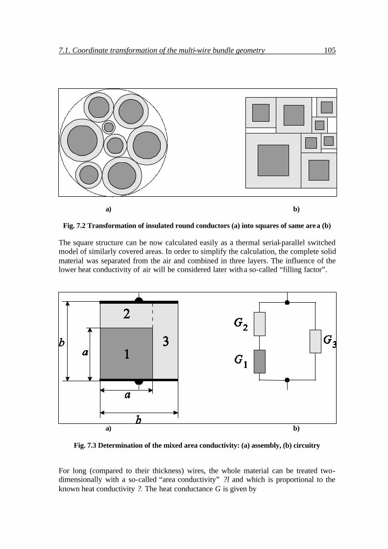
7.1. Coordinate transformation of the multi-wire bundle geometry 105
a) b)
Fig. 7.2 Transformation of insulated round conductors (a) into squares of same area (b)
The square structure can be now calculated easily as a thermal serial-parallel switched model of similarly covered areas. In order to simplify the calculation, the complete solid material was separated from the air and combined in three layers. The influence of the lower heat conductivity of air will be considered later with a so-called “filling factor”.
a) b)
Fig. 7.3 Determination of the mixed area conductivity: (a) assembly, (b) circuitry
For long (compared to their thickness) wires, the whole material can be treated two-dimensionally with a so-called “area conductivity” ?l and which is proportional to the known heat conductivity ?. The heat conductance G is given by

106 Chapter 7. Calculation of the heat transfer in a multi-wire bundle
ylx
Gλ
=
and for each layer given in Fig.3 one obtains:
lG λ= , lG 11 λ= , ab
alG
−= 22 λ ,
bab
lG−
= 33 λ (7.2)
Finally, a “Mixed Material Equation” of the following form is obtained:
+−−+
= 11
1
1
22 b
a
ab
λλ
λλ (7.3)
where the heat conductance are replaced by their heat conductivities. here: ? radial mixed heat conductivity, ?1 heat conductivity of the conductor, ?2 heat conductivity of the wire insulation (see Fig.7.1), a edge of heat conduc tor material 1 (?1), in mm, b edge of mixed heat conductor material 1 and 2 (?) in mm. The next step is to determine the relationship of b/a which is calculated from the area a2 of the materials 1 and 2 (which is the cross section of the conductor and the isolator). Since the conductor consists of single wire veins with air gaps in between, the real con-duction cross section a2 has still to be multiplied with the so-called filling factor f , which is the relationship of the real conducting cross section to the cross section to be determined by its measured diameter: A1= a2 f. The cross section of the conductor and the isolator together results in:
22
1 bAf
A=+ (7.4)
from which finally b/a can be calculated, whereby the areas A2 and A1 may be replaced by the sums of the diameter squares of the conductor d and of the wire veins δ:
Σ==
+=
∑
∑ f
n
df
AfA
ab
i
ii
i
i
1
2
1
2
1
2 1δ
(7.5)

7.1. Coordinate transformation of the multi-wire bundle geometry 107 The model described by the equation 7.3 is only valid for materials with similar heat conductivity. If one part diverts as far as air compared to copper, the model is no longer applicable. In this case, the assumption is made, that the conductor consists of two dif-ferent conducting materials, which are switched in parallel as follows: G = Ga + Gb.
Fig. 7.4 Volume change due to empty spaces, in accordance with the filling factor f or F In accordance with Fig. 7.4 the heat conductivities can be calculated as follows:
λ=G , bc
G aa λ= ,b
cbG ab
−= λ (7.6)
here: ? mixed heat conductivity, ?a, ?b heat conductivity of area a2 and b2, respectively, a, b virtual length of all conductors and of mixed conductor, c virtual length c/b of b2. Replacing a square element by two rectangular elements with different heat conductiv-ity, (see Fig. 7.4) leads to the mixed heat conductivity:
bcb
bc
ba−
+= λλλ .
Using the filling factor:
bc
f =
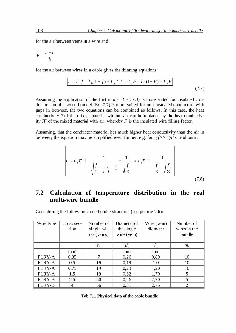
108 Chapter 7. Calculation of the heat transfer in a multi-wire bundle for the air between veins in a wire and
bcb
F−
=
for the air between wires in a cable gives the thinning equations:
FFFfff abaaba λλλλλλλλ ≈−+=≈−+= )1(,)1( (7.7)
Assuming the application of the first model (Eq. 7.3) is more suited for insulated con-ductors and the second model (Eq. 7.7) is more suited for non- insulated conductors with gaps in between, the two equations can be combined as follows. In this case, the heat conductivity ? of the mixed material without air can be replaced by the heat conductiv-ity ?F of the mixed material with air, whereby F is the insulated wire filling factor. Assuming, that the conductor material has much higher heat conductivity than the air in between, the equation may be simplified even further, e.g. for ?1f>> ?2F one obtains:
Σ−
Σ
+≈
Σ
−−+
Σ
+=ff
Ff
ff
F1
11
1
11 2
1
22 λ
λλ
λλ
(7.8)
7.2 Calculation of temperature distribution in the real multi-wire bundle Considering the following cable bundle structure, (see picture 7.6): Wire type
Cross sec-
tion Number of single wi-res (veins)
Diameter of the single wire (vein)
Wire (vein) diameter
Number of wires in the
bundle
ni δ i ∂i mi
mm2 mm mm FLRY-A 0,35 7 0,26 0,80 10 FLRY-A 0,5 19 0,19 1,0 10 FLRY-A 0,75 19 0,23 1,20 10 FLRY-A 1,5 19 0,32 1,70 5 FLRY-B 2,5 50 0,26 2,20 5 FLRY-B 4 56 0,31 2,75 2
Tab 7.1. Physical data of the cable bundle

7.2. Calculation of temperature distribution in the real multi-wire bundle 109 First, calculating the fill factor f of the wire:
2
2
∂=
δnf
(7.9) here: ? wire diameter in mm From the conductor and wire vein squared sum data, a cross section quotient Σ of cable bundle is calculated:
∑
∑
∑
∑==Σ i
ii
i
iii
i
i
i
ii
dm
nm
d
n
1
2
1
2
1
2
1
2 δδ
(7.10) Since, experiment data are available of the cable bundle presented in the 7.1 table, the bundle fill factor of cable bundle F empirically can be calculated:
( )21
2
4
SUU
IlF
S π
ρπ
−⋅Σ=
(7.11) Finally, having all required information to calculate radial averaged heat conduction co-efficient ?, Eq. (7.8) can be used to obtain this coefficient:
Σ
−−
Σ
+=ff
F1
1
112λλ
(7.8)
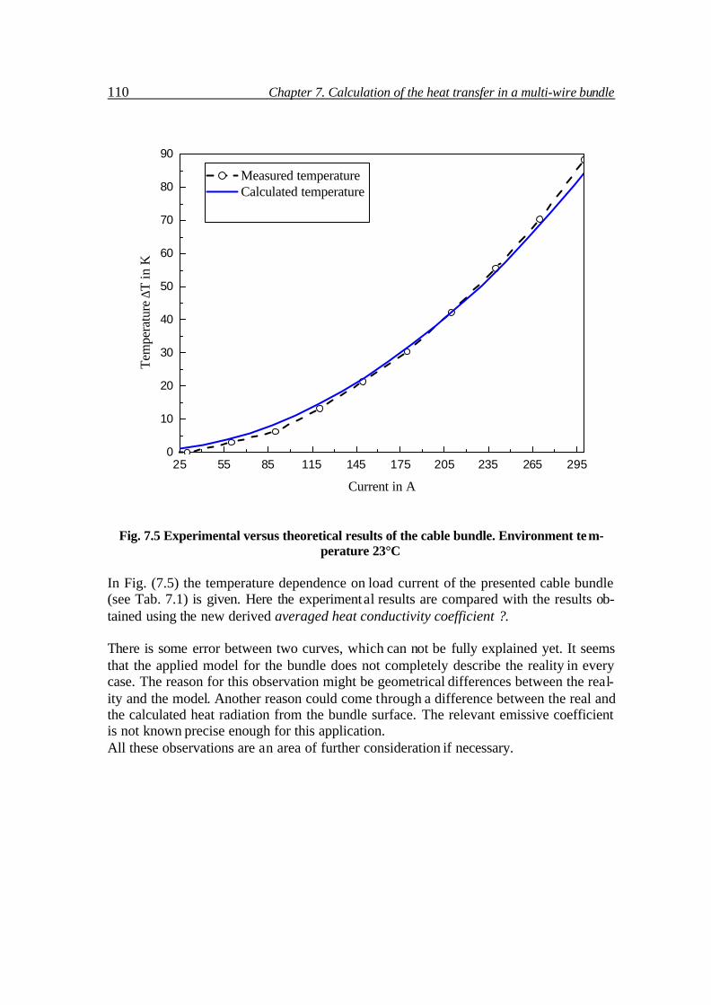
110 Chapter 7. Calculation of the heat transfer in a multi-wire bundle
25 55 85 115 145 175 205 235 265 2950
10
20
30
40
50
60
70
80
90
Measured temperature Calculated temperature
Tem
pera
ture
∆T
in K
Current in A
Fig. 7.5 Experimental versus theoretical results of the cable bundle. Environment tem-perature 23°C
In Fig. (7.5) the temperature dependence on load current of the presented cable bundle (see Tab. 7.1) is given. Here the experimental results are compared with the results ob-tained using the new derived averaged heat conductivity coefficient ?. There is some error between two curves, which can not be fully explained yet. It seems that the applied model for the bundle does not completely describe the reality in every case. The reason for this observation might be geometrical differences between the real-ity and the model. Another reason could come through a difference between the real and the calculated heat radiation from the bundle surface. The relevant emissive coefficient is not known precise enough for this application. All these observations are an area of further consideration if necessary.

7.2. Calculation of temperature distribution in the real multi-wire bundle 111
Fig. 7.6 Experimental setup of multi-wire bundle Despite of all these small errors, the results of the calculations are more than sufficient for practical applications.

________________
CHAPTER 8 ________________ SUMMARY AND
CONCLUSIONS 8.1 Summary Heat transfer and temperature distribution in electrical cables and fuses have been stud-ied analytically and numerically in the present research work. Obtained results from numerical simulation are interpolated by the Least-Square method that led to simple polynomial and logarithmical functions of the main thermo-electrical characteristics. The geometries of physical models and appropriate heat trans fer equations are presented in Chapter 2. Analytical solutions of the heat equations for different conductor types have been obtained in Chapter 3. A numerical approach based on a finite volume method has been studied in Chapter 4. A new computational algorithm to compute tran-sient state thermo-electrical characteristics of electrical cables was also described in Chapter 4. The experimental setup and the execution procedure of the experiments is explained in Chapter 5. The achieved computational results of the developed mathe-matical model were verified by laboratory experiments. Interpolation using Least-squares technique of numerical results in order to reduce the amount of numerical data is given in Chapter 6. Finally, a new approach to calculate heat conduction coefficient of multilayer cable bundles is presented in Chapter 7. The ultimate goal of this work is to develop a methodology of the analysis of heat trans-fer in electrical cables and fuses. The main result of this analysis is: temperature distri-bution in the conductors and transient state thermo-electrical characteristics. To obtain these steady- / transient-state characteristics a numerical algorithm had to be employed, since most materials are temperature dependant. Another reason for a use of numerical algorithm is that the heat transfer calculation is much easier to perform by a numerical approach instead of applying analytical Fourier series solutions. A one-dimensional model for different kinds of electric conductors is presented in sec-tion 2.2. The physical models of three different types of conductors: flat cable, round wire and fuse melting element are taken as physical examples for mathematical model-ling, simulation and analysis of heat transfer. When creating the mathematical models (section 2.3) the heat transfer equations were reduced to one-dimensional problems (Eq. 2.3, 2.6, 2.7). In order to have a clear understanding about the modelling of the heat transfer in electric conductors the entire second chapter is devoted to the derivation of a mathematical model. Therefore, sections 2.4, 2.5 describe the analysis of heat conduc-tion and thermal convection respectively. Since, one has to deal with an initial-boundary
114 Chapter 8. Summary and conclusions value problem, boundary conditions are described in section 2.6. Here are the first kind (Dirichlet) and mixed type (symmetry and convective-radiative) limit conditions are presented. Additionally, numerical implementation of the same kind of boundary cond i-tions is given in section 4.3.2. After creation and preparation of the mathematical model of electric conductors the fo l-lowing Chapters 3 and 4 give detailed analysis of analytical and numerical calculation procedures of temperature distribution in the conductors. In the analytical analysis (Chapter 3), exact solutions of steady state heat transfer equa-tions were obtained. These solutions are given for temperature independent material co-efficients as well as for temperature dependent coefficients. Different boundary cond i-tions (symmetry or derived from energy balance equation) were implemented for ana-lytical expressions. A very important property was obtained from the heat equation with temperature dependant coefficients. This property is called “avalanche effect” and can be described by the following equation: if,
A
IIEu
20
0
ρααα ρ
ρ == (3.53)
then,
∞=∞= AA T,χ . The next step of heat transfer analysis in the electric conductors was to develop a nu-merical model to compute steady- and transient-state temperature behaviour in the con-ductors. The numerical model was created using a finite volume method. The integral form of the heat equation was discretised using central differences in space and a back-ward difference scheme in time. Thus, second order accuracy scheme in space and first order accuracy in time was achieved. Discretisation of the equations in time were made implicitly in order to achieve unconditional stability and increase computational effi-ciency. All finite volume schemes were developed on structured grids, however this method is straightforward applicable on unstructured grids too. Systems of algebraic equations were solved by the iterative Newton-Raphson method, which has fast conver-gence if a suitable initial guess is made. As computational results, fo llowing characteristics were obtained (Fig. 6.10, 6.11-6.14, Chapter 6): a) conductor surface temperature as a function of load current, b) heating up time as a function of load current, c) time constant as a function of load current, d) electric field strength as a function of load current (considering non- linear electric resistance dependence on temperature) e) temperature distribution in the fuse element.
8.1 Summary 115 Chapter 5 details how the theoretical model of electric cables and fuses has been tested. For this purpose, two different experiments (section 5.1.1 and 5.1.2) were made. The first experiment deals with the determination of the temperature coefficient of cop-per resistance. This coefficient is an important parameter for the determination of the cable resistance dependence on temperature. Three different cables were placed in a heated liquid silicon bath. The cable conductor resistance change due to temperature was measured. Necessary theory was developed and described in the section 5.1.1. The experimental set up is described in section 5.2. The second experiment was designed to measure the cable power dissipation. Here, all available wires and cables as well as fuses and cable bundles were connected to the di-rect current power supply source and loaded with the power from 0 to the maximal al-lowed value. The whole experiment was controlled by the software developed for this purpose. The necessary theory of this experiment and experimental setup are given in the sections 5.1.2 and 5.2 respectively. The measuring process and the parameter acqui-sition procedure was described in the section 5.3. Chapter 6 describes the validation of the mathematical model of electric conductors and the interpolation procedure of the numerical results by simple polynomial functions. The validation of the model was based on estimating the parameters, which most influ-ence the heat transfer in electric cables. Therefore, considerable attention was paid to the validation of the heat convection coefficient, α, and the temperature coefficient of copper resistance, αρ. From section 6.1 one could see that the mathematical model was properly derived and approximated, since characteristics presented in figures 6.3, 6.4, 6.6, 6.7, 6.9 have good agreement with experimental data. In section 6.2 an algorithm was developed to interpolate numerical results. All thermo-electrical characteristics were interpolated by simple polynomial functions using the Least-Square method. These functions are very useful for practical calculation problems of electric cables. Also, if such equations are implemented in the computer programme to calculate thermal performance of electric cables, the programme gives very good computational efficiency in time. The polynomial functions are given in Eq. (6.7-6.9). The final chapter concludes this study with a newly developed approach of heat transfer calculation in the multi-wire cable bundle. This chapter applies the principles, which have been derived for single conductors to multi-wires. Only after detailed research of heat transfer models for single wires and cables was it possible to derive the methodol-ogy for the cable bundle. The key of this methodology is to calculate averaged heat conductivity coefficient of multi-wire layers. Therefore, it was proposed to use the lin-ear coordinate transformation in order to simplify cable bundle geometry. An averaging method for layered media was then used to determine a mixed or averaged heat conduc-tivity coefficient. The cable bundle model is given in Fig. 7.1 and its transformation to square frames of the same area in Fig. 7.2. Developed “mixed material equations” for thermal conductivity coefficient is given by the Eq. 7.3. In the following section 7.2 the comparison of the results was given. They were obtained with the calculated mixed heat

116 Chapter 8. Summary and conclusions conductivity coefficient and compared with measurements from the cable bundle. From the figure 7.5, one could see that the developed method to calculate the averaged heat conductivity coefficient gives sufficient accuracy for practical applications. 8.2 Conclusions Four different one-dimensional analytical and numerical models were successfully de-veloped in this research work, which are able to simulate heat transfer in any kind of electric conductors such as flat cables, round electric wires, electric fuses or multi-wire cable bundles. The new analytical-numerical approach, which has been proposed in this work, allows analysis of the thermo-electrical characteristics of electric conductors. From this study, several other conclusions are as follows: Ø Analytical solutions for steady-state temperature distribution in a single con-
ductor were obtained. These solutions are valid for temperature independent material constants as well as temperature dependant material constants. An “avalanche effect” has been obtained from these analytical solutions (section 3.3.3). It was also observed that transient heat transfer equations require very complicated techniques which are time and space dependent in order to obtain exact solutions. Therefore it is not worth making too much effort to solve tran-sient heat transfer equations. Instead, a numerical approach should be used.
Ø A numerical model as developed to simulate heat transfer in the conduc tors,
which is based on the finite volume method. This simulates heat transfer very precisely due to the scheme of second order in space. Also implicit schemes in time proved to have better computational performance than explicit ones if time accuracy is not of primary importance.
Ø Experiments delivered qualitative data and enabling an estimate of the qua lity
of the mathematical model. Ø A new method to calculate heat transfer in the multi-wire cable bundle was
created. Original equations of heat conductivity coefficient were used by trans-forming the complicated wire bundle geometry to more simple squares. Equa-tions of “mixed material properties” produce averaged heat conductivity coef-ficients for a cable bundle, which consist of materials as copper, PVC and air.
Ø An analytical-numerical approach was developed to simulate heat transfer in
electric conductors. This was implemented into a computer aided design pro-gram to optimise thermal performance of the cables.
Ø The developed software allows analysis of thermo-electric properties of both
wires and fuses. This analysis is very important for fuse manufacturing proc-esses in order to obtain better time-current characteristics for wire and cable protection against overload and short-circuit currents. In the future, companies
8.2. Conclusions 117
could design fuse materials, using the developed software. The result would be very narrow time-current characteristic of a fuse (close to wire time-current characteristic). Finally, wires and cables can be loaded with 100% load while being protected by the fuses in a reliable way.
Ø The main results of this study were presented in three international conferences
(Lithuania, 2003) and published in three international journals. List of publications: 1. A. Ilgevicius, H.D. Liess. Thermal Analysis of Electrical Wires by Finite Volume Method. Electronics and Electrical Engineering. Nr. 4 (46), Kaunas, 2003. 2. A. Ilgevicius, H.D. Liess. Calculation of the Heat Transfer in Cylindrical Wires and Fuses by Implicit Finite Volume Method. Mathematical Modelling and Analysis, 8(3), 217-227, 2003. 3. H.D.Liess, A. Ilgevicius. Analytical versus Numerical Solutions of Physical Prob-lems. The Benefits of its Combination. Mathematical Modelling and Analysis, 8(4), 291-302, 2003. 8.3 Suggestions for future research In the present research a one-dimensional model for different geometries of physical models have been developed. However a two-dimensional model would be appreciable for heat transfer simulation in complicated fuse element geometries and multi-wire bun-dles. Also, a mesh generation tool for Cartesian and radial coordinates is desirable.

118 Chapter 8. Summary and conclusions
Fig. 8.1. Multi-wire tree of on-board electrical system
More research work should be undertaken developing mathematical models of cable bundles or even cable trees (see Fig. 8.1). Heat conductivity inside the bundle has to be estimated by further experimental works in order to validate the numerical model. Stud-ies should also be made to ascertain which numerical method is more appropriate for the model for cables bundle and cable trees: finite volume or finite element method.
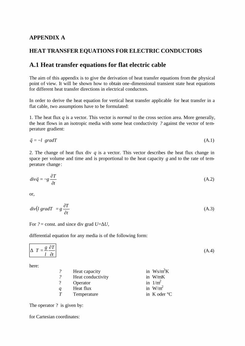
APPENDIX A HEAT TRANSFER EQUATIONS FOR ELECTRIC CONDUCTORS A.1 Heat transfer equations for flat electric cable The aim of this appendix is to give the derivation of heat transfer equations from the physical point of view. It will be shown how to obtain one-dimensional transient state heat equations for different heat transfer directions in electrical conductors. In order to derive the heat equation for vertical heat transfer applicable for heat transfer in a flat cable, two assumptions have to be formulated: 1. The heat flux q is a vector. This vector is normal to the cross section area. More generally, the heat flows in an isotropic media with some heat conductivity ? against the vector of tem-perature gradient:
gradTq λ−=r
(A.1) 2. The change of heat flux div q is a vector. This vector describes the heat flux change in space per volume and time and is proportional to the heat capacity γ and to the rate of tem-perature change :
tT
qdiv∂∂
−= γr
(A.2)
or,
( )tT
gradTdiv∂∂
= γλ (A.3)
For ? = const. and since div grad U=∆U, differential equation for any media is of the following form:
tT
T∂∂
=⋅∆λγ
(A.4)
here:
? Heat capacity in Ws/m3K ? Heat conductivity in W/mK ? Operator in 1/m2 q Heat flux in W/m2 T Temperature in K oder °C
The operator ? is given by: for Cartesian coordinates:

120 Appendix A. Heat transfer equations for electrical conductors
2
2
2
2
2
2
zyx ∂∂
+∂∂
+∂∂
=∆
for cylindrical coordinates:
2
2
22
2
2
2 11ϕ∂∂
+∂∂
+∂∂
+∂∂
=∆rrrrx
dPy
Fig. A.1 Vertical heat transfer in the flat cable
According to the picture in A1, electric power Pe is given by: dPe = O E J dy (A.5) In z- direction the heat power Pz can be neglected: Pz = 0 (A.6) In y- direction the heat power through the cable surface is as follows:
dytydT
OPy),(
λ−= (A.7)
In the cable accumulated heat energy Q:
( )dytyTOdQ ,∆= γ (A.8) here: O = a l is the surface area in m2 From the energy balance equation, Pe is given by:

A2. Heat transfer equations for round electric wire 121
dtdQ
PP ye += or
+=dtdQ
ddPdP ye (A.9)
By inserting the equations A.5, A.7 and A.8 to the equation A.9, we obtain a differential equation for transient temperature distribution in the flat cable:
( )dy
dttyT
dOdy
tyTdOdyJEO
+−=
),(,2
γλ (A.10)
dividing by O⋅ dy:
( )0
),(,2
2
=∂
∂⋅−+
∂∂
ttyT
JEy
tyTγλ (A.11)
or,
( )0
),(,2
2
=∂
∂⋅−+
∂∂
ttyTJE
ytyT
λγ
λ (A.12)
A.2 Heat transfer equations for round electric wire For radial heat transfer, differential equations with cylindrical coordinates have to be used. In figure A.2 heat conduction is given.
Fig. A.2 Radial heat transfer in the round wire
Electric power Pe is given by: dPe = O E J dr (A.13)

122 Appendix A. Heat transfer equations for electrical conductors where: O = l u = 2 p l r - the surface dPe = 2 p l r E J dr (A.13a) Radial heat power of the wire Pr is given by:
drtrdT
rldr
trdTOPr
),(2
),(λπλ −=−= (A.14)
drtrTd
rldrdr
trdTldPr
),(2
),(2
2
λπλπ −−=
In the wire accumulated heat energy Q:
( ) ( )drtrdTrldrtrdTulQd ,2,2 γπγ == (A.15) From the energy balance equation, for radial heat conduction, the power Pr is given by:
dtdQ
PP re += or
+=
dtdQ
ddPdP re (A.16)
After insertion of the equations A.13a, A.14 and A.15 into the equation A.16, the differential equation for transient temperature distribution in the cylindrical wire follows:
( ) ( )dr
dttrT
rldr
trTdrltrdTldrJErl
),(2
,2,22
2
γπλπλππ +−−= (A.17)
divided by 2π l r dr we have,
( ) ( )0
),(,,2
2
=∂
∂⋅−+
∂∂
+∂
∂t
trTJE
rrtrT
rtrT
γλλ (A.17a)
or,
( ) ( )0
),(,,2
2
=∂
∂⋅−+
∂∂
+∂
∂t
trTJErr
trTr
trTλγ
λ (A.18)

A3. Heat transfer equations for electric fuse element 123 A.3 Heat transfer equations for an electric fuse element Here we consider axial heat transfer in a cylindrical or flat body electric fuse with constant cross section. The axial heat conduction in a cylindrical fuse element is given in picture A.3.
Fig. A.3 Axial heat transfer in the fuse
According to Fig. A3, electric power Pe is given by: dPe = A E J dx (A.19) Radial heat conduction Pr through the surface is: dPr = a u T(x,t) dx (A.20) Axial heat conduction Px along the fuse is::
dxtxdT
APx),(
λ−= (A.21)
In the wire accumulated heat energy Q is:
( )dxtxTAdQ ,γ= (A.22) From the energy balance equation, Pr is given by:
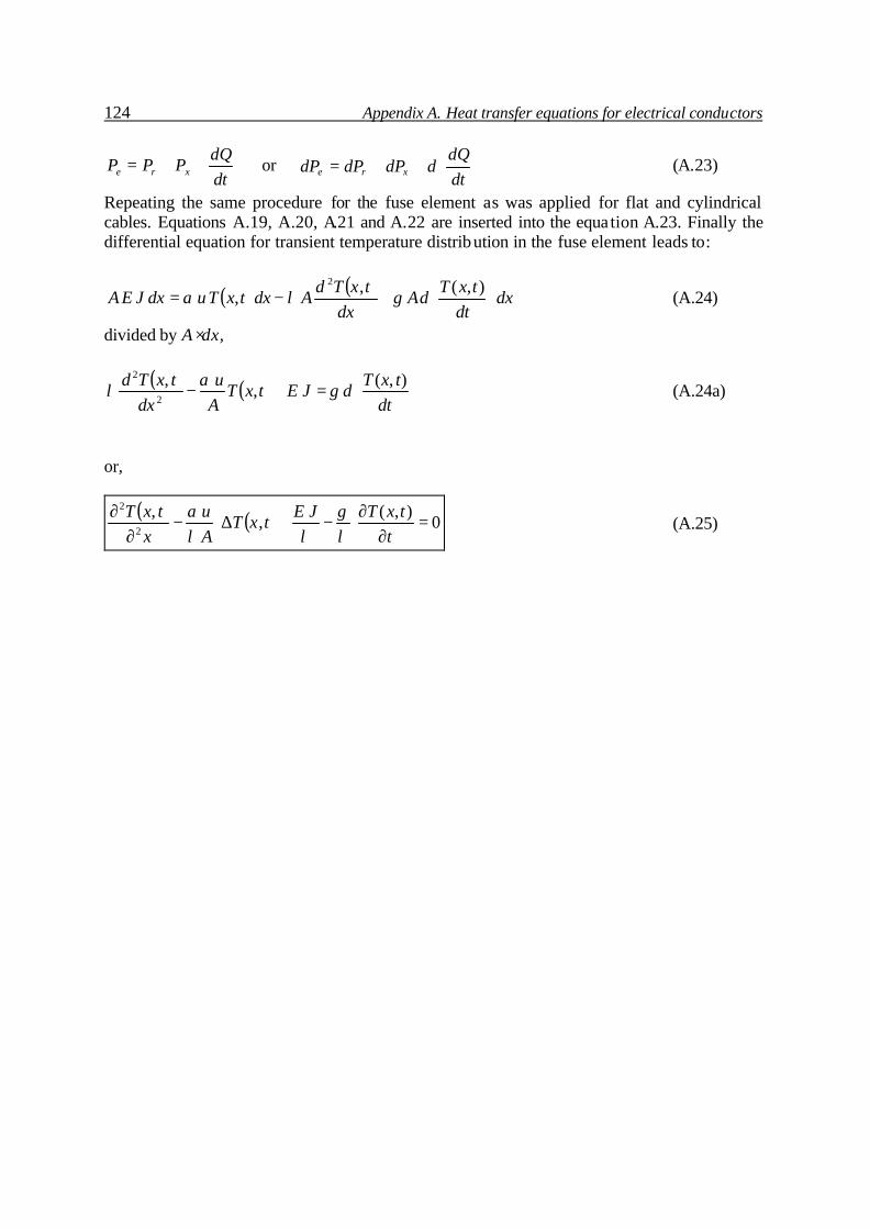
124 Appendix A. Heat transfer equations for electrical conductors
dtdQ
PPP xre ++= or
++=
dtdQ
ddPdPdP xre (A.23)
Repeating the same procedure for the fuse element as was applied for flat and cylindrical cables. Equations A.19, A.20, A.21 and A.22 are inserted into the equation A.23. Finally the differential equation for transient temperature distribution in the fuse element leads to:
( ) ( )dx
dttxT
dAdx
txTdAdxtxTudxJEA
+−=
),(,,
2
γλα (A.24)
divided by A ⋅ dx,
( ) ( )
=+−
dttxT
dJEtxTAu
dxtxTd ),(
,,
2
2
γα
λ (A.24a)
or,
( ) ( ) 0),(
,,
2
2
=∂
∂⋅−+∆⋅−
∂∂
ttxTJE
txTAu
xtxT
λγ
λλα
(A.25)

APPENDIX B NUMERICAL ALGORITHM APPLICATION FOR HEAT TRANSFER SIMULATION B.1 Numerical heat transfer simulation and interpolation of the results The aim of this appendix is to illustrate the practical implementation of a numerical algorithm (Chapter 4) in order to simulate the heat transfer in electric conductors and the implementa-tion of the interpolation algorithm (Chapter 6). In the figure B.1 the graphical interface to input pre-processing data for the numerical simulation of heat transfer in cylindrical wires is given. Here the user has the possibility to choose any geometry of the wire in cylindrical co-ordinates, environment temperature and to apply different types of materials. The boundary conditions are, however, fixed, and expose free convection and radiation to the air. As post-processing information, numerical representation in an ASCII file (see Fig. B.2). Interpola-tion results are saved in the binary file (see Fig. B.3)
Fig. B.1 Window of pre -processing information for the heat transfer simulation program in cylindrical wires

126 Appendix B. Numerical algorithm application for heat transfer simulation
Fig. B.2 Simulation data of a cylindrical wire with 10mm2 cross section. Here: I1 – load current in amps, T1 – conductor surface temperature in °C, E1 – electrical field strength in V/m, tau –
time constant after n=5 in sec, tg – heating up time to reach 90°C in sec. B.2 Calculation of thermo-electric characteristics by the polynomial functions In order to be able to work with an interpolated mathematical model or with simplified poly-nomial functions, another programme was created (see Fig. B4). Here, using equations (6.7-6.10) given in section 6.2, thermo-electrical characteristics can be calculated.

127 B.2. Calculation of thermo-electrical characteristics by the polynomial functions
Fig. B.3 Binary file, where all interpolation coefficients are saved (A, B, C, D, Tau).

128 Appendix B. Numerical algorithm application for heat transfer simulation
Fig. B.4 Programme, which calculates thermo-electrical characteristics of cylindrical wire by simplified polynomial functions.

APPENDIX C SOFTWARE FOR MEASUREMENT DATA ACQUISITION C.1 Algorithm description and measurement program In the section 5.3 two different measurement procedures of electric cables to validate the mathematical model were explained. In this appendix, a closer look at the measurement soft-ware will be given. Both experiments were run by the same type of software, implemented in the LabView 6.1 environment. For the explanation in this chapter, only the second experiment software will be presented. This program controls the power supply of direct current and digi-tal multimeter, to which the measurement sensors were attached. The control of measurement equipment is implemented by a GPIB controller. The program has the following structure:
- set the voltage to 15V; - open the files needed to save the results and the computations; - reset the multimeter; - write into the files the date and the time; - compute R65 – in order to do this: apply a 1 amp current for 60 seconds, read the voltage
drops on the cable and on the shunt, read the environment temperature and finally com-pute it;
- for all current values (for i = 0 to number of currents do): o compute the present current and apply it to the cable; o for j = ’number of measurements’ – 4 to ‘number of measurements’ do:
§ set the multimeter scale to DC voltage range; § read the voltage drop on the shunt and wait for 4 seconds – also save the
value in a variable; § read the voltage drop on the cable and wait for 4 seconds – also save the
value in a variable; § read the sensor temperature - read actually a voltage drop and then com-
pute the temperature with the following formula: Ts = 2.83668 + 15.5669 * VoltageDrop * 1000.
Remark: this thermocouple sensor is a safety sensor, which cuts off the power supply if the conductor temperature exceeds maximal allowed value.
§ read the environment temperature and save the value in a variable for later use.
§ based on the saved values compute the cable resistance, the cable tem-perature, the cable power.
§ write the results in the file dedicated to computed values. - write into both files the date and the time (the measurement has finished at this point); - reset both power supply and multimeter; - close both files;
The program interface is shown in the picture C.1.

130 Appendix C. Software for measurement data acquisition
Fig. C.1 Measurement programme to measure cable voltage drop, resistance, electric power and
temperature
The measurement of cable resistance, voltage drop, electric power and temperature can be started if all measurement equipment defined in the programme is switched on. The program should initialise the available GPIB controller, power supply source, temperature sensors and the digital multimeter, which serves as a data acquisition device. Whenever the hardware is correctly initialised, the user should give initial data into the program. First, “Strom für R0” box has to be filled in, where some current value required in order to measure cold resistance R0 of the cable. Next, in the box “Shuntwiderstand” shunt resistance should be defined in order to compute exact load current produced by the power supply. “Alpha20” box defines the temperature coefficient of copper resistance. This value is required for the temperature computation of the cable. “Temperatur Limit” required for the safety reasons, if the cable temperature exceeds this value, the power supply source is cut off. “Min. Strom” and “Max. Strom” are required to specify the starting current load value and the end current value re-spectively. Next, the step size of measurement interval should be given. For this, the box “Strom-Intervall” should be used. The measurement time, after which the steady state should be reached is given in the box “Messzeit pro Strom”. The box “Anzahl Messungen” means, how many intermediate values for every measurement interval should be measured and saved in the file. This information is important in order to record the transient state of cable tem-perature. The measurement procedure then begins, and the whole experiment runs automatically. In order to observe the measurement data online, the computer with measurement software should be connected to the Ethernet network, and using “Remote Desktop Connection” application, the measurement computer can be controlled via the Ethernet network. On the right hand side of the program, online measurement information is presented: actual load current, actual cable temperature obtained by measuring cable voltage drop, cable surface temperature

C.2. Measurement results 131 obtained by thermocouple sensor, environment temperature obtained by Pt100 sensor and the cold cable resistance R0. C.2 Measurement results The measurement programme produced numerical results, saved in the ASCII type file (see Fig. C.2)

132 Appendix C. Software for measurement data acquisition
Measure
ment Tim
e
Speci
al Even
ts
Measure
d Cabl
e Tem
p
Wanted
Curren
t
Curren
t mea
sured
by Po
werSup
ply
calcul
ated c
urrent
Cable P
ower
Shunt
Voltag
e Drop
Cable V
oltage
Drop
Cable
Resist
ance
48 16:11 - Extra file initiated as: C:\CPOW\testfin.log48 16:11 - Environment temperature: 20.00000 deg C0 16:11 - User Tom Roida startet a new Measurement! Date: 2001-4-2
16 16:11 - Setting new current to 0.00 A515 33,76 0 0,36 0,12250 0,00039 2,45000E-05 3,19790E-03616 33,61 0 0,36 0,12150 0,00039 2,43000E-05 3,19450E-03716 33,47 0 0,29 0,12300 0,00039 2,46000E-05 3,19430E-03816 33,29 0 0,29 0,12050 0,00038 2,41000E-05 3,19080E-03876 16:26 - Setting new current to 10.00 A
1416 33,17 10 9,87 9,68050 1,89056 1,93610E-03 1,95296E-01 2,01741E-021516 33,17 10 9,87 9,67950 1,89034 1,93590E-03 1,95293E-01 2,01760E-021616 33,17 10 9,94 9,67950 1,89036 1,93590E-03 1,95295E-01 2,01762E-021716 33,13 10 9,94 9,67950 1,89017 1,93590E-03 1,95276E-01 2,01741E-021736 16:40 - Setting new current to 20.00 A2316 33,98 20 19,96 19,72500 7,85852 3,94500E-03 3,98404E-01 2,01979E-022416 34,15 20 19,96 19,72500 7,86177 3,94500E-03 3,98569E-01 2,02063E-022516 34,31 20 19,96 19,72400 7,86573 3,94480E-03 3,98790E-01 2,02185E-022615 34,46 20 19,96 19,72300 7,86993 3,94460E-03 3,99023E-01 2,02314E-022649 16:55 - Setting new current to 30.00 A3216 36,24 30 29,91 29,69550 17,95414 5,93910E-03 6,04608E-01 2,03603E-023315 36,33 30 29,98 29,69650 17,95839 5,93930E-03 6,04731E-01 2,03637E-023416 36,38 30 29,98 29,69550 17,96082 5,93910E-03 6,04833E-01 2,03678E-023516 36,46 30 29,98 29,69500 17,96533 5,93900E-03 6,04995E-01 2,03736E-023616 36,50 30 29,91 29,69300 17,96810 5,93860E-03 6,05129E-01 2,03795E-023616 17:11 - Setting new current to 40.00 A4316 37,73 40 40 39,74350 32,25896 7,94870E-03 8,11679E-01 2,04229E-024416 37,47 40 40 39,74350 32,23397 7,94870E-03 8,11050E-01 2,04071E-024516 37,27 40 40 39,74500 32,22366 7,94900E-03 8,10760E-01 2,03990E-024615 37,18 40 40 39,74700 32,21542 7,94940E-03 8,10512E-01 2,03918E-024636 17:28 - Setting new current to 50.00 A5315 38,61 50 49,94 49,72800 50,73365 9,94560E-03 1,02022E+00 2,05161E-025416 38,48 50 49,94 49,72700 50,72164 9,94540E-03 1,02000E+00 2,05120E-025516 38,62 50 50,02 49,72800 50,75503 9,94560E-03 1,02065E+00 2,05247E-025616 38,73 50 49,94 49,72750 50,78436 9,94550E-03 1,02125E+00 2,05370E-025716 38,83 50 49,94 49,72650 50,83431 9,94530E-03 1,02228E+00 2,05580E-025716 17:46 - Setting new current to 60.00 A6516 42,00 60 60,04 59,78150 74,50084 1,19563E-02 1,24622E+00 2,08462E-026616 42,07 60 60,04 59,78200 74,51892 1,19564E-02 1,24651E+00 2,08509E-026715 42,08 60 59,96 59,78100 74,53166 1,19562E-02 1,24675E+00 2,08552E-026816 42,17 60 60,04 59,78150 74,54066 1,19563E-02 1,24689E+00 2,08574E-026843 18:05 - Setting new current to 70.00 A7716 44,92 70 69,98 69,76700 102,64526 1,39534E-02 1,47126E+00 2,10882E-027816 44,94 70 69,98 69,76750 102,66071 1,39535E-02 1,47147E+00 2,10910E-028015 45,01 70 69,98 69,76800 102,67282 1,39536E-02 1,47163E+00 2,10932E-028023 18:25 - Setting new current to 80.00 A8916 48,16 80 80 79,81350 136,04219 1,59627E-02 1,70450E+00 2,13560E-029016 48,07 80 80 79,81350 136,03437 1,59627E-02 1,70440E+00 2,13548E-029116 48,31 80 80 79,81250 136,07361 1,59625E-02 1,70492E+00 2,13615E-029216 48,17 80 80,08 79,81300 136,06273 1,59626E-02 1,70477E+00 2,13595E-029256 18:45 - Setting new current to 90.00 A
10216 51,48 90 89,95 89,74750 174,35920 1,79495E-02 1,94278E+00 2,16471E-0210316 51,50 90 89,95 89,74750 174,40156 1,79495E-02 1,94325E+00 2,16524E-0210416 51,45 90 89,95 89,74900 174,38087 1,79498E-02 1,94298E+00 2,16491E-0210516 51,48 90 89,95 89,74800 174,38144 1,79496E-02 1,94301E+00 2,16496E-0210543 19:07 - Setting new current to 100.00 A11516 54,99 100 99,97 99,86350 219,14446 1,99727E-02 2,19444E+00 2,19744E-0211616 55,12 100 100,04 99,86500 219,07785 1,99730E-02 2,19374E+00 2,19671E-0211716 55,14 100 100,04 99,86400 219,10461 1,99728E-02 2,19403E+00 2,19702E-0211816 55,10 100 100,04 99,86600 219,06106 1,99732E-02 2,19355E+00 2,19649E-0211883 19:29 - Setting new current to 110.00 A12922 58,88 110 109,84300 269,33833 2,19686E-02 2,45203E+00 2,23230E-0213016 58,81 110 109,99 109,84450 269,30137 2,19689E-02 2,45166E+00 2,23194E-0213116 58,81 110 110,06 109,84200 269,27327 2,19684E-02 2,45146E+00 2,23181E-02
Fig. C.2 Saved experimental data in ASCII type file
in Win A in Ain A
in °C
in V
in V
in ohm

C.2. Measurement results 133
Cable Power & Resistance
0
100
200
300
400
500
600
700
800
900
1000
1100
1200
0,00 20,00 40,00 60,00 80,00 100,00 120,00 140,00 160,00 180,00 200,00
Current in A
Po
wer
in W
0,019000
0,020000
0,021000
0,022000
0,023000
0,024000
0,025000
0,026000
0,027000
Res
ista
nce
in O
hm
Cable power
Cable Resistance
Polynomisch (Cable power)
Polynomisch (Cable Resistance)
Fig. C.3 Measured cable power and resistance after steady state regime
11900 12000 12100 12200 12300 12400 12500 12600 1270090
91
92
93
94
95
96 Experimental data Fitted by exponential function
Tran
sien
t sta
te c
able
tem
pera
ture
T in
°C
Measurement time t in s
Fig. C.4 Measured cable surface temperature in transient state regime at the current I = 170 A

Bibliography [1] Hiranandani, Ajit. Calculation of Conductor Temperatures and Ampacities of
Cable Systems Using a Generalized Finite Difference Model. IEEE Transactions on Power Delivery, Vol. 6, No. 1, 15-21, January 1991.
[2] Haskew, Tim, A., Carwile, Regina F., Grigsby, L., L. An Algorithm for Steady-State Thermal Analysis of Electrical Cables with Radiation by reduced Newton-Raphson Techniques. IEEE Transactions on Power Delivery, Vol. 9, No. 1, January 1994.
[3] Harshe, B.L., Black, W.Z. Ampacity of cables in single open-top cable trays. IEEE Transactions on Power Delievery, Vol. 9; No. 4, October 1994.
[4] El-Kady, M.A. Calculation of the power cable ampacity to variations of design and environment parameters. IEEE transactions on power and systems. Vol. PAS-103; No.8, 2043-2050, 1984.
[5] Ryan, C., Leen, G. and Heffernan, D. A Prototype Steer-by-Wire and Brake-by-Wire System for Educational Research Projects. Proceeedings U.K. Institute of Physics - Sensors&Applications XII. Sept. 2003.
[6] Neher, J.H, McGrath, M.H. The Calculation of temperature Rise and Load Capability of Cable Systems. AIEE Transactions, Vol. 76, 752-772, October 1957.
[7] George J. Anders. Rating of electric power cables. IEEE Press Power Engineering Series. McGraw-Hill, 1997. ISBN 0-7803-1177-9.
[8] Schulz, Thomas. Grundsatzuntersuchung zum Temperaturverhalten elektrischer Leitungen und deren Schutzelemente auf Schmelztleiterbasis in Kfz-Bordnetzen. Dissertation, Universität der Bundeswehr München, 2002.
[9] Das, S., Knapp, R. H. and Shimabukuro, T.A. Finite Element Analysis - A New Tool for Cable Design. Proc 50th Intl. Wire and Cable Symposium, Paper 11-4, Lake Buena Vista, FL, Nov. 12-15, 2001.
[10] Groth, C., Müller, G. FEM für Praktiker-Temperaturfelder. Band 463, Expert Verlag, 2. Auflage, 1997.
[11] Incropera, Frank, P., DeWitt, David P. Introduction to heat transfer. John Willey & Sons, USA, 1985. ISBN 0-471-80126-7.
[12] Buikis, A., Kalis, H. The mathematical modelling of nonlinear heat transport in thin plate. Mathematical modelling and analysis, Vol. 4, 44-50, 1999.
[13] Kalis, H. Lasis, A. Simple algorithms for calculation of the axial – symmetric heat transport problem in a cylinder. 6(2), 262-269, 2001.
[14] Buikis, A., Kalis, H. Calculation of electromagnetic fields, forces and temperature in a finite cylinder. Mathematical modelling and analysis, 7(1) 21-32, 2002.
[15] Zurbau, O. Optimizing the wire system package in automobile industry. Diplom thesis, Universität der Bundeswehr München, 2002.
[16] Tslaf, Avraham. Combined properties of conductors. Physical science data Vol. 9, Elsevier, Netherlands, 1981. ISBN 0-444-41959-4.
[17] VDI-Wärmeatlas, 8. Auflage, Springer-Verlag, Berlin, New York, 1997. ISBN 3-540-62719-7.
[18] Wongyala, Nawin. Erwärmung elektrischer Leiter. Diplomarbeit, Universität der Bundeswehr München, 1999.

136 Bibliography [19] Özsik, M.,N. Finite difference methods in heat transfer. CRC Press, Inc., USA,
1994. ISBN 0-8493-2491-2. [20] Zienkewic, O.C. The finite element method in Engineering Science. New York:
McGraw-Hill. 1971. [21] Gottlieb, D., Orszag, S. A. Numerical Analysis of Spectral Analysis: Theory and
Applications, Society for Industrial and Applied Mathematics. Philadelphia, PA, 1977.
[22] Versteeg, H.K, Malalsekera, W. An introduction to computational fluid dynamics. The finite volume method. Longman Group, 1995. ISBN 0-582-21884-5.
[23] Hirsch, C. Numerical computation of internal and external flows. Vol.1: Fundamentals of numerical discretization. ISBN 0-471-91762-1.
[24] Mack, P. Bestimmung des linearen und quadratischen Temperaturkoeffizienten ausgewählter elektrischer Leiter. Studienarbeit, Universität der Bundeswehr München, 2001.
[25] Roida, T. Automatisierte Messung der Wärmeableitung von elektrisch beheizten Leitern. Studientarbeit, Universität der Bundeswehr München, 2001.
[26] Lancaster, P., Šalkauskas. K. Curve and surface fitting. An introduction. Academic press, UK, 1986. ISBN 0-12-436060-2.
[27] Cuthbert, D., Fred, S.W. Fitting equations to data. John Wiley & Sons, USA, 1980. ISBN 0-471-05370-8.
[28] Chien-Ching, Shin-Wen Chang. Analytical exact solutions of heat conduction problems for anisotropic multilayered media. International journal of heat and mass transfer 47, 1643-1655, 2004.
[29] Fletcher, C.A. Computational Galerkin methods. New York, Berlin, Heidelberg, Tokyo, Springer Verlag, 1984.
[30] Munoz-Cobo, J.L, Corberan, J.M, Chiva, S. Explicit formulas for laminar natural convection heat transfer along vertical cylinders with power-law wall temperature distribution. Heat and Mass Transfer 39, 215-222, 2003.
[31] Kays, W.M., Crawford, M.E. Convective Heat Transfer. Mc Graw Hill, 1993. [32] Anders, G.J., Roiz, J., Moshref, A. Advanced computer programs for power cable
ampacity calculations. IEEE Comput. Appl. Power, Vol. 3, No. 3, 42-45, 1996. [33] El-Kady, M.A. Calculation of the sensitivity of power cable ampacity to variations
of design and environmental parameters. IEEE Trans. Power App. Syst., Vol. PAS-103, No. 8, 2043-2050, 1985.
[34] Flatabo, N. Transient heat conduction problem in power cables solved by the finite element method. IEEE Trans. Power App. Syst. Vol. PAS-92, 161-168, 1973.
[35] Hanna, M.A., Chikhani, A.Y., Salama, M., M., A. Thermal analysis of power cables in multi-layered soil. Parts 1 and 2. IEEE Trans. Power Delivery, Vol. 8, No. 3, 761-778, 1993.
[36] Kellow, M.A. A numerical procedure for the calculation of temperature rise and ampacity of underground cables. IEEE Trans. Power App. Syst., Vol. PAS-100, No. 7, 3322-3330, 1981.
[37] Mushamalirwa, D., Germay, N., Steffens, J.C. A 2-D finite element mesh generator for thermal analysis of underground power cables. IEEE Trans. Power Delivery, Vol. 3, No. 1, 62-68, 1988.
[38] Cannon, J.R. The one-dimensional heat equation. Addison-Wesley Publishing Company, USA, 1984, ISBN 0-201-13522-1.
[39] Shneider, P.J. Conduction heat transfer. Addison-Wesley,Reading, MA, 1955.

Bibliography 137 [40] Burmeister, L.,C. Convective Heat Transfer. 2nd Ed., Wiley, New York, 1995. [41] Simson, J.R. Engineering heat transfer. The Macmillan Press Ltd, 1975. ISBN 0
333 18757 1. [42] Shih, Tien-Mo. Numerical properties and methodologies in heat transfer. Springer-
Verlag, Berlin, 1983. ISBN 0-89116-309-3. [43] Lisejkin, V.D. Grid generation methods. Springer-Verlag Berlin Heidelberg New
York. 1999. ISBN 3-540-65686-3. [44] Heinhold, L. Kabel und Leitungen für Starkstrom. Teil 1 und 2. Siemens Verlag, 4.
Auflage 1987. [45] Bauer, H. Kraftfahrtechnisches Taschenbuch. Bosch, 22. Auflage-VDI-Verlag,
1995. ISBN 3-18-419122-2. [46] Al-Khafaji, Amir Wadi. Numerical methods in engineering practice. Saunders
College Publishing, 1986. ISBN 0-03-001757-2. [47] Morton, Keith W. Numerical solution of convection-diffusion problems.
Chapman&Hall, 1996. ISBN 0 412 56440 8. [48] Jaluria, Y. Computational heat transfer. Springer-Verlag, 1986. ISBN 3-540-
16879-6. [49] Müller, G. FEM für Praktiker. Expert Verlag,1993. ISBN 3-8169-0800-4. [50] Lax, P. D. Calculus with application and computing Vol.1. Springer-Verlag. 1976.
ISBN 3-540-90179-5. [51] Minkowycz, W.J. Handbook of numerical heat transfer. John Wiley & Sons,
Inc,1988, ISBN 0-471-83093-3. [52] Ansorge, R. Iterative solution of nonlinear system equations. Proceedings of a
Meeting held at Oberwolfach, Germany, Jan. 31-Feb. 5. Springer-Verlag, 1982. ISBN 0-387-11602-8.
[53] Shih, Tien-Mo. Numerical heat transfer. Springer-Verlag, 1984. ISBN 3-540-13051-9.
[54] Mitchell, A.R. The finite difference method in partial differential equations. John Willey & Sons, 1985. ISBN 0 471 27641 3.
[55] Anderson, D. A. Computational fluid mechanics and heat transfer. Hemisphere publishing corporation, New York, 1984. ISBN 0-89116-471-5.
[56] Tveito, A. Introduction to partial differential equations. Springer-Verlag, 1998. ISBN 0-387-98327-9.
[57] Ganzha, V.G. Numerical solutions for partial differential equations. Problems solving using Mathematica. CRC Press, Inc., 1996. ISBN 0-8493-7379-4.
[58] Tyn, M.U. Partial differential equations for scientist and engineers. Elsevier Science Publishing Co., 1987, ISBN 0-444-01173-0.
[59] Stephenson, G. Partial differential equations for scientists and engineers. Longman, 1980. ISBN 0-582-44696-1.
[60] VVedensky, D. Partial differential equations with Mathematica. Adison-Wesley, 1993. ISBN 0-201-54409-1.
[61] Baehr, H. D. Heat and Mass Transfer. Springer, New York , 1998. [62] Bejan, A. Heat Transfer. John Wiley, New York, 1993. [63] Incropera, F. and DeWitt, D. Heat and Mass Transfer. John Wiley, 2nd Ed.,1985. [64] Suryanarayana, N.V. Engineering Heat Transfer. West Pub. Co., Minneapolis/St
Paul, 1995. [65] Carslaw, H.S. and Jaeger, J.C. Conduction of Heat in Solids. Clarendon
Press,Oxford, UK, 1959.
138 Bibliography [66] Grigull, U. Heat Conduction. Springer-Verlag, New York; Hemisphere Pub Corp.,
Washington, D.C., 1984. [67] Poulikakos, D. Conduction Heat Transfer. Prentice Hall, Englewood Cli_s, NJ,
1994. [68] Kaviany, M. Principles of Convective Heat Transfer. Springer-Verlag, New York,
1994. [69] Oosthuizen, P.H. and Naylor, D. Introduction to Convective Heat Transfer
Analysis. McGraw-Hill, 1998. [70] Modest, M.F. Radiative Heat Transfer. McGraw-Hill, New York, 1993. [71] Myers, G.E. Analytical Methods in Conduction Heat Transfer. McGraw-Hill, New
York, 1971. [72] Adams, J.A., Rogers, D. F. Computer-Aided Heat Transfer Analysis. McGraw-Hill,
New York, 1973. [73] Wang, Z.J. Spectral (Finite) Volume Method for Conservation Laws on
Unstructured Grids. Journal of Computational Physics, 178, 210-251, 2002. [74] Ciegis, R. Diferencialiniu lygciu skaitiniai sprendimo metodai. Kaunas, 2003. ISBN
9986-05-588-1. [75] IEEE Standart Power Cable Ampacity Tables, IEEE Std 835, 1994. [76] Calculation of the Continuous Current Rating of Cables (100% load factor). IEC
Publication 287, 1982 and subsequent editions. [77] A Method for Calculating Reduction Factors for Groups of Cables in Free Air,
Protected from Solar Radiation. IEC Publication 1042, 1991. [78] Buikis, A.,Ulanova, N. Analytical-numerical method for temperature fields in
multilayered system. Advanced Computational Methods in Heat Transfer, VI, Sauthappton, Boston: WITp, 445-453, 2000.
[79] Abou khachfe, R., Jarny, Y. Determination of heat sources and heat transfer coefficient for two-dimensional heat flow-numerical study. Int. J. Heat Mass Transfer 44(7), 2001.
[80] Cai, R.X., Zhang, N. Some algebraically explicit analytical solutions of unsteady nonlinear heat conduction. Int. J. Heat Transfer. ASME 123(6), 2001.
[81] Chang, C.Y., Ma, C.C. Transient thermal conduction analysis of a rectangular plate with multiple insulated cracks by the alternating method. Int. J. Heat Mass Transfer 44(13), 2001.
[82] Chen, B.S., Gu, Y.X., Guan, Z.Q., Zhang, H.W. Nonlinear transient heat conduction analysis with precise time integration method. Numer. Heat Transfer Part B-Fundamentals 40 (13), 2001.
[83] Asllanaj, F. Jeandel, G., Roche, J.R. Numerical solution of radiative transfer equation coupled with nonlinear heat conduction equation. Int. J. Numer. Meth. Heat Fluid Flow 11 (5–6),2001.
[84] Krishnaprakas, C. K. Combined Conduction and Radiation Heat Transfer in a Cylindrical Medium. Journal of Thermophysics and Heat Transfer, Vol. 12, No. 4, 605-608, 1998.
[85] Talukdar, P., Mishra, S. C. Transient conduction and radiation heat transfer with variable thermal conductivity. Numerical Heat Transfer, Part A, 41: 851-867, 2002.

Acknolegment This dissertation has been written during my activity as a research engineer in the Insti-tute of Physics of Electrical Engineering and Information Technology Faculty of Uni-versity of the Bundeswehr Munich. I would like sincerely to thank Prof. Dr. H.-D. Ließ for accepting me to his research group and confiding this topic to me. His interest on the progress of my research work, supervision and provided support had been valuable help for me. I wish to express my deep gratitude to Prof. Habil. Dr. R. Ciegis, who kindly agreed to supervise my Ph.D. dissertation in numerical heat transfer subject and gave me an inten-sive course on the mathematical modelling topic. I thank also Prof. R. Ciegis for his contribution as the second reviser of this work. Prof. Habil. Dr. H. Dalichau I thank for the revision of this work as the third reviser. His remarks and suggestions on computer aided computational techniques were very valu-able for me. I would like to thank Prof. Dr. K. Landes for his contribution as the chairman of the ex-amination committee and beyond it for interesting discussions about the research work. I wish to acknowledge valuable discussions with the Prof. Dr. R. Rinkeviciene, Prof. Habil. Dr. A.J. Poska, and Prof. Habil. Dr. A. Smilgevicius from Vilnius Gediminas Technology University, Faculty of Electronics during preparation the dissertation manuscript. I acknowledge valuable support of Dipl. –Ing. M. Glinka and Dipl.-Ing. M. Hiller from EIT 6 and Dr.-Ing. T. K. Wurst from LRT 10 for providing expensive laboratory equipment. Without this equipment would not had been possible to validate the research theory. The co-workers and colleagues from my research team I deeply thank for the assistance with the programming of numerical algorithms and measurement software. Last but not least, the technical staff from LRT 6 I thank for the help to set up the meas-urement equipment. Finally, but most deeply, I thank my parents, without whose constant encouragement, support, assistance, and tole rance this dissertation would not have been possible.