Volume 139, number 5,6 PHYSICS LETTERS A 7 August 1989

ANALYTIC GENERATING FUNCTION FOR T H E BRILLOUIN SPECTRUM

Manmohan SINGH 3072/2B/2, St No. 22, Banjtt Nagar, New Delht 110008, Indta

Received 14 November 1988; accepted for pubhcation 18 May 1989 Communicated by A.R. Bishop

A umque analytic generating function IS derived for the Brllloum spectrum with the central Raylelgh line, by using the formal- lsm given earher by the author. The utlhty of this generating function to study the time-interval statistics of the Brllloum spectrum is also shown.

1. Introduction

The slow development of the field photon-counting statistics (PCS) of Gaussian light is mainly due to the inadequately developed mathematical structure underlying the given problem. However, with the sustained interest of a few (!) researchers, closed-form solutions of certain long standing problems have now started to appear (see refs. [ 1-7 ] for example).

In this paper we solve yet another long standing problem of practical interest for thefirst tlrne, namely, the PCS of the Brillouin spectrum with the central Rayleigh line via its unique one-fold generating function (g.f.) derived here on the lines of the author's formalism given in refs. [4,7 ].

Inelastic light scattering from the molecular vibrations in fluids and from the elementary excitations of con- densed matter like phonons or magnons, results in a Brillouin-Mandelstam spectrum (scattering from acoustic phonons/magnons) . The frequency A and the wave vector k of the quasiparticle are defined by the laws of conservation of energy and momentum:

oas=co,+A, k s = k , + k ( I k s l ~ l k , I ) , (1)

where the s and i respectively signify the scattered wave and the incident wave. The fine structure of the scat- tered light consists of three lines - the central Rayleigh line with two Brillouin components, symmetrically placed around it. The ratio of the intensity of the central line Ro to that of the two shifted lines 2R_+ 1, as determined by the thermodynamic fluctuation theory (see ref. [ 8 ] ) is given by

rl=Ro/2R±, =Cp/C~ - 1, (2)

where Cp and Cv are the specific heat at constant pressure and volume respectively. The constant t/is generally known as the Landau-Placzek ratio [ 8 ]. Generally, the intensity of the Brillouin components is quite poor as compared to the intensity of the Rayleigh line. For example in p-methoxy benzylidene p-(n-butylaniline) (MBBA) Clark and Liao [9] report this ratio to be of the order of 102-104.

A study of the half-width of the central Rayleigh line provides us with a means of studying the thermal dif- fusivity of the scattering medium, whereas the study of the side lobes provides us with a means of determining the sound velocity in the scattering medium [ 8 ]. Interesting details of the various experimental techniques employed to study the Brillouin frequencies are given in a review article of Borovik-Romanov and Kreines [ 10 ] and recent papers of Simonsohn and co-workers [ 11,121- However, the important question that we need to address in such a study is: how to distinguish between the pure Brillouin (two-peaks) and the Brillouin with

0375-9601/89/$ 03.50 © Elsevier Science Publishers B.V. 213 (North-Holland Physics Publishing Division )

Volume 139, number 5,6 PHYSICS LETTERS A 7 August 1989

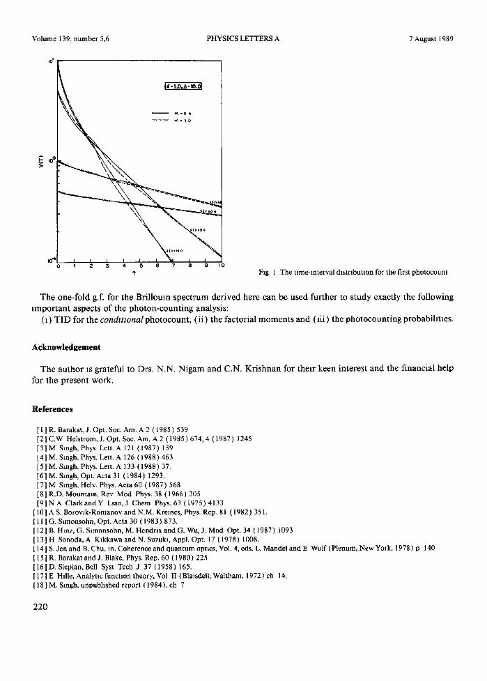
central Raylelgh line (three peaks) cases? The answer is obviously manifest in the different "correlation-times" in these two cases. In the one-fold photon-counting analysis like the time-interval statxstms here, this task can be easily accomplished by a simple experimental set up consisting of time-to-amplitude-converter (TAC) and pulse-hmght analyser (PHA) measuring time intervals with a resolution of the order of I 0- 6_ 10- 7 s (see refs. [ 13,14 ] ). In section 5 (fig. 1 ), we show that there is indeed a clear difference between the time-interval dis- tributlons (TIDs) followed by the two- (pure Brlllouin) and the three-packed (Brillouln with Rayleigh com- ponent) spectra.

The power spectrum of this three-peaked spectrum is given by Barakat and Blake [ 15 ] as

' ~ , , In (3) I(oJ) = ,--~-i R, (o9_o9,)2+y 2 ,

and if the total intensity is normalized to umty, we have

; l R , = I . (4) I(to) d~o= ,=-Y~I

The field-correlation g(z) of the scattered light is given by [ 15 ]

g ( r ) = ( 1 -o~)e- i r l +e-•lrl cos/'IT= ( 1 -o~)e -I~t + ½t~(e -plrl +e-#'l~l ) , (5)

where

f l = a - i A , f l*=6+iA, (6)

c ~ = 2 R _ ~ = 2 R + ~ = I - R o ( 0 ~ a ~ < l ) , (7)

a = y l / y o = ~ - l / ~ o . (8)

The parameter A represents the frequency shift, ot the fraction of energy in the Brillouin lines and ~ is the ratio of the BriUouin and Rayleigh half-widths. Interestingly, Barakat and Blake [ 15 ] call c~ in eq. (7) the Landau- Placzek ratio! The following relationship of r/and a is evident from eqs. (2) and (7),

o:= 1/(1 +~/). (9)

2. The Fredholm integral equation

Central to the study of the PCS of Gaussian light is the solution of the following Fredholm integral equation of the second kind, so as to finally obtain the sought g.f. for a given spectrum:

T

s ] gl t - t ' l e~k( t ' ) dt' = 2 k ~ k ( t ) , ( 10)

0

where s is a useful parameter, g l t - t' I the field-correlation and Ok (t) and 2 k represent the eigenfunctions and the eigenvalues respectively.

The one-fold g.f. for Gaussian light is related with the eigenvalues of eq. (10) in the following way,

Q(s, T ) = I-I ( l + s ( I ) 2 k ) - l (11) k

Substituting eq. (5) into eq. (10), we get

214

Volume 139, number 5,6 PHYSICS LETTERS A

T

s j [ ( 1 - c t ) e - i t - c I + ½cz(e -~ l t -c I + e -a*lt-t'l)O(t' ) dt' = 2 0 ( 0 • (12) 0

To solve eq. (12) we follow ref. [ 16 ]. Differentiat ing eq. (12) six t imes with respect to t, we get

p6 +Ap4 + Bp2 +C=O , (13)

where

A = ( S ~ a l - 1)- - (fl*E+fl 2) , B=s~,(aE-al)+(fl*2+flE)(s;~al- 1) +fl*2fl 2 ,

C=s~(a3 -a2 ) -s~(a2 - a l ) (fledt 2.~ fiE) .~ (s~al - 1 )flit 2p2 ,

with

al = 2 [ l - a + ½ a ( f l * + f l ) ] , a2 =2[1-0~+ ½0~(p*3+p3)],

a a = 2 [ l - a + ½ a ( f l * 5 + f l s ) ] , ~ = 1 / 2 . (14)

Eq. (13 ) above suggests the following simple form of the eigenfunctions Ù(t),

0( t ) = A t e P t + A E e - m . (15)

Now we proceed to solve eq. (13) exactly. First we notice that as the coefficients of eq. (13) are all real, the roots of eq. (13) will occur in conjugate pairs. Also evident is the fact that if p, is a solution then - p , is also a solution. Putting pE=x in eq. (13 ), we get the following cubic equation,

x3 +Ax2 + Bx+ C=O , (16)

which is solved exactly by using Cardan 's formula which converts eq. ( 16 ) into the following equation first,

ya + uy+ v=o , (17)

where

x = y - A / 3 , U = B - A 2 / 3 , V = C - A B / 3 + 2 A 3 / 2 7 . (18)

The roots of eq. (18) are given by

Y I = A + B , yz=toA+to2B, y3=toEA+toB,

where

A = ( V / 2 + x / ~ ) w 3 , B = ( V / 2 - v / - R ) t / 3 , R = V 2 / 4 + U 3 / 2 7 , (19)

m = ( - 1 + i v / 3 ) / 2 , ta2= - (1 + i x / ~ ) / 2 .

Thus the six roots of eq. (14) as determined by eqs. ( 18 ) and (19) , are

P, = + (x,) I/2= + ( Y , - A / 3 ) ~/2 • (20)

The nature of the p, above will help us in determining the mult.iple-valued nature of the Fredholm-deter- minant ( F D ) as we shall see in section 3.

Following the details o f ref. [4] (for example) , we solve eq. (12) on substituting eq. (15) in it,

7 August 1989

215

Volume 139, number 5,6 PHYSICS LETTERS A 7 August 1989

!

s[ ( ! [(1-ot)e-t+CWIol(e-flt+flC-be-#*t+~c)]

7

-b f [ (1-oL)et-C + loL(ePt-l~C-beP*t-g*C) l)(AlepC-bA2e-pC) dt' 3 t

=2(AlePt+A2e-pt) . (21)

Putting 1 - a = a l , a/2=a2 and integrating eq. (21) we get

s[OtlA~ ( 1 -p)Z2(p)Z3(P)e-t(e (t+p)'- 1 ) +a~A2( 1 +p)Z2(p)Z3(p)e-t(e (~-p)t- 1 )

-[-oL2A 1 ( f l - - / 3 ) Z 1 (p)Z3(p)e-/St(e (,e+p)t_ 1 ) +ot2A2(fl+p)Zl (p)Z3(P)e -at(e (lS-p)t_ 1 )

+ a2A~ ( / ~ - P ) Z t (p)Z2(p)e-~'t( e(~ +P)t- 1 ) + a2A2(,/3* + p)Z~ (p)Z2(P)e-a*t(e ~#*-p)l_ 1 )

+a~At ( 1 +p)Z2(P)Z3(p)et(e-(l-P)t-e -(~-p)r) +a~A2( 1 -p)Z2(P)Z3(p)e'(e-~+P)~-e -~l+p)r)

+a2A~ (fl+ p)Z~ (p)Z3(p)e/s~(e-(~a-p)t-e-us-p)r) +a2A2(~-p)Z~ (p)Z3(p)e~at( e-ce+p)t-e -(,a+p)r)

+a:A~ (/3* + p)Z~ (p)Z2(p)ea*t( e-(a*-P)t-e -(#*-p)v)

q- ot2A 2 (fl* - p ) Z , (p)Zz (p)ea'~(e - (#*+p)t_ e - (#*+P)r) ]

=2Z, (p ) ZE (P ) Z3 (P ) ( A ,eP' + A2e -pt ) ,

where

Z t ( p ) = l - p 2, Zz(p)=flZ-p 2, Z3(p)=/3*2-p 2. (22)

Now, on collecting the coefficients o fe +t, e+pt and e -+#*t in eq. (22), we obtain the following FD D(~) for the non-singular solution:

D(~) =

R,(pl) R , ( -pL)E, (p , , T) Rz(pt) R2(-pl)Ez(p, , T) R3(pl ) R, ( - p , ) R1 (p,)El ( --Pl, T) R 2 ( - p , ) RE(p~ )E2( - P l , T) R 3 ( - p l )

RI(P2) R~(-pz)E~(p2, T) RE(p2) R2(-p2)E2(p2, T) R3(P2) R~( -p2 ) RI(pz)E~(-p2, T) R2(-P2) Rz(p2)E2(-p2, T) R3(-p2)

Rt (P3) RI ( -P3)EI (P3, T) Rz(p3) R2( -p3)E2(p3, T) R3(P3) R I ( - p 3 ) RI(p3)EI(-p3, T) R2( -P3) R2(p3)Ez(-p3, T) R3(-P3)

where

R,(p) = (/3, +p)Z(p) ,

with

i l l = l , f lz=fl , ]~3=ff g , Z(p)=Zj (p)Zk(p) ,

where t,j , k = l , 2, 3 and t~ j~k . On putting ~=0 in eq. (23), we get

D(0) = 26f12fl*2 ( 1 _fiE) 2(fl .2_ f12) 2(//*2_ 1 )2.

E,(p) =exp[ - (fl, + p ) T ] ,

R3( - P l )E3(Pl, T) R3(Pl )E3( - P t , T) R3 ( -192)E3 (P2, T) R3(P2)E3(-P2, T) ' R3( -p3)E3(P3 , T) R3(P3)E3(--P3, T)

(23)

(24)

(25)

216

Volume 139, number 5,6 PHYSICS LETTERS A 7 August 1989

3. Non-analytic behaviour of FD

As we aim to obtain the sought g.f. by using Hadamard's theorem [ 17 ] we have to first ensure that the FD D(~) obtained above (eq. (23)) is an entire function.

To see the multiple-valued character of the FD, let us first see how the roots in eq. (20) change into each other, if we go around a complete circle in the complex l-plane. For this we represent A and B in eq. (19) as

A = (rle '°) 1/3, B = (r2e - '°) i/3 (26)

If we go around a complete circle, we see the following changes in A and B respectively,

A= (rle '°) 1/3 0~0+2n, "1~'1/3'~'0/3+21n/3~'1/3~"0/3'~ --'1 " ( - -½+l ix /~ ) =toA,

B = (r2e -,0) ,/3 0~0+ 2,% r~/3e -,0/3--2,~:/3= _r~/3e-,O/3( ½ + ½ix/~) =to2B. (27)

Consequently, we see that

Yl = A + B 0~o+2% t .oA+co2B=y2. (28)

Similarly, we can see that

Yl = A + B 0~o+4~ O.)2A+(.oB=y3, or y2=t.oA+092 B o~o+2n (.02A+f~B=y3. (29)

Thus, YI, Y2 and Y3 act as three different branches of the FD D(~)in eq. (23). The second reason for the multiple-valuedness of the FD stems from the fact that the ordering of the p, in

eq. (23) is completely arbitrary and as a result, we have sign flippings in the FD whenever p , ~ - p , or p,-op: (t:/:j). Thus, if we divide or multiply the FD D(~) by a factor p~ P2P3, we obtain a function, say P(~), free from the multiple-valuedness,

P(¢) =D(~)p, P2P3, (30)

or

P( ¢) = D( ¢) /pl P2 P3 . (31)

Further, we investigate D(¢) for its singular behavlour in the complex e-plane. This can happen whenever the roots Pl, P2 and Ps satisfy the following equations,

P2=--+P2, P2=+--p3, p3=--+pt , (32)

on some axis. Eq. (32) results whenever

C + A 3 / 2 7 = 0 , (33)

as can be easily seen from eqs. (16) - (20) . Eq. (33) in turn implies the following cubic equation in ~,

~ 3 - A ' ~ 2 + B ' ~ - C ' = 0 , (34)

where

A ' = ( 3 / a l ) ( l + f l * z + f l 2) , B '=(1 /a3)[2- -] f l f l* ( f l*+f l+f l f l* ) -3a~( l+f l*2+B2)] ,

C ' = (1 /a 3) [(1 +fl,2+f12) 3+27fl,2f12 ] . (35)

As earlier, eq. (34) can be solved by converting it to the following equations first,

¢3+U'¢+ V' = 0 , (36)

217

Volume 139, number 5,6 PHYSICS LETTERS A 7 August 1989

where

~ = ~ + A ' / 3 , U'=B'+A'2/3, V '=-C '+A 'B ' /3+2A '3 /27 .

The roots of eq. (36) are given by

¢~ =A' + B ' , ¢2 =ooA' +co2B ' , ¢3 =o92A' +coB' , (37)

where

A'=(V'/2+xf-R)~/3, B'=(V' /2_x/-R) ' /3 , R '=V'2/a+u'3/27.

Thus eq. (37) completely determines the points at which D(~) becomes singular in the complex Splane. Eq. (32) suggests that we have to divide D(~) by a factor (p~ - p ~ ) (p~ - p ] ) (p] - p ~ ) . For consistency with

the other possible exchanges amongst the p,, we need to consider the factor (p~ _p~)2(p~ _p])2(p] _p~)2. However, the uniqueness of the sought g.f. can be determined only from the following boundary conditions,

l<~Q(s, T)~< 1, (38)

O(s,T)ls=o= ~ (1-s)~P(n,T) l~=o=l , (39) n=0

( - 1 )cgQ(s, T)/Osls=o= <n>, (40)

as formulated by the present author in refs. [4-7 ].

4. The unique analytic g.f.

We can render the given FD to be an analytic function, say M(~), by defining it as follows (see refs. [4,7] for example):

M( ~)=P( ~) /f( ~) , (41)

where P(~) is a single-valued function determined by eq. (30) or ( 31 ) andf(~) determines the exact functional form of the singularities in the FD D(~). This function f(~) has to satisfy the following condition,

f(~)lp,=+_pj=O ( t , J = l , 3 ; t # J ) . (42)

For determining the exact functional form of unique analytm g.f. for the Bnllouin spectrum, the following dis- cussion is necessary.

Once we have ensured the function M(~) to be analytic in nature, we are in a position to apply Hadamard's theorem [17]. As the order [17] of the entire function M(~) is at most ½ (as can be easily seen from eqs. (20) and (23)) , we can represent it by the following infinite product,

M(~) = M ( 0 ) 1-'[ (1 - ~ / ~ k ) , (43) k

where M(0) is a constant. Now Hadamard's theorem [ 17] implies that the infinite products in eq. ( 11 ) and eq. (43) can equated, on being of the same order [ 17 ]. Thus, we get

Q(s, T) =M(O)/M( - <1> ). (44)

The importance of the form of the g.f. in eq. (44) stems from the fact that we have completely bypassed the explicit evaluation of the eigenvalues of eq. (10), as would become imperative on employing eq. ( 11 ).

Next, it follows from the arguments for the case of two-peaked spectra discussed in refs. [4,7 ] that we aban- don the choice of P(~) in eq. (30), as in such a case the very idea of multiplying or dividing the FD D (~) by the factor p~ P2P3 would be lost! Choosing the form of P(~) given in eq. (31), eq. (40) requires that

218

Volume 139, number 5,6 PHYSICS LETTERS A 7 August ! 989

l ( ~ (Of/Op,)lm=l.m=t~.,3=~)=4[(l+]3)_,+(,8.+,8)_,+(,8.+l)_l] (45) f (0 ) ,=l

The functions satisfying both eqs. (42) and (45) are given as

f(P~,P2,P3)= ,~JVI I (p2 -pJ:)2 (flz _ fl2)2 exp ~ -(-~z _---~jz) :,] j (f(O)=e'), (46)

and

(p,: _py)2 f(Pl,P2, P3)= ,I-I,,j (fl2_fl~): ( f (o) = 1 ) , (47)

where i, j = 1, 3 and i~j . The choice in eq. (46) has to be abandoned as it violates the condition of eq. (38) (on being divergent in nature!). However, the choice in eq. (47) satisfies eq. (38), as we obtain

Q(s, T) Ir=o = 1. (48)

Eq. (48) carries a very important fact namely: " i f there are any singularities in the FD D(~), then eq. (48) would remain violated but in turn will give us the exact nature of the singularities in D(~)!".

Thus the unique analytic g.f. for the Brillouin spectrum with the central Rayleigh line is now given by eqs. (23) - (25) , (41), (44) and (47) and its dtrect dependence on the spectral parameters c~ and ci, A comes via eqs. (6) and ( 13 ) respectively. The explicit functional form of the g.f. for this three-peaked spectrum can be obtained by using the present author's method of expanding a determinant [ 18 ], though the task is more in- volved here, unlike the case of two-peaked spectra discussed in refs. [4,7 ].

5. T ime- in terva l s ta t i s t i c s

The probability densxty of registering the first photocount V(T) is defined as [ 13 ]

V(T) = ( I ( T ) exp [ -sE(T) ] ) . (49)

Using the well-known fact that the g.f. can be expressed as follows:

Q(s, T) = (exp[ -sE(T) ] ) , (50)

where E(T) =f~ I(t' ) dt' and l(t) is the instantaneous intensity of the scattered field, we can re-express V(T) as

V(T) = -OQ(s, T)/OTIs=, . (51)

It is evident from eq. (51 ) that the functional dependence of the TID V(T) on the spectral parameters a, 6, A comes through the g.f. Q(s, T) given by eqs. (23 ) - (25 ) , (41), (44) and (47). Fig. 1 shows the behaviour of the TID V(T) for the first photocount. The TIDs for the two- (oe = 1.0 ) and three-peaked (oe = 0.4) spectra are clearly distinguishable from each other. We notice an interesting feature here that unlike the ease of the two-peaked spectrum characterizing a polydisperse medium discussed in ref. [4], we see the emergence of "kinks" in the present case of the Brillouin spectrum. We attribute these "kinks" to the cos Jz factor in the auto-correlation for the Brillouin spectrum given in eq. (5). However, the curves for ct = 0.4 (three peaks) are much flatter than the curves for ot = 1.0 (two peaks). This is due to the central Rayleigh line - the dominant component in the or=0.4 case! We also confirm that at the origin ( T = 0 )

V(T) lr=o= (I) ,

as in the polydispersity ease discussed in ref. [4].

(52)

219

Volume 139, number 5,6

iO j

PHYSICS LETTERS A 7 August 1989

E Io ° >

IO -I : 0 t 2 3 4 5 6 7 8 9 I 0

T Fig 1 The time-interval &stnbutlon for the first photocount

T h e one- fo ld g.f. for the Br i l l oum s p e c t r u m d e r i v e d here can be used fu r ther to s tudy exact ly the fo l lowing

~mpor tant aspects o f the p h o t o n - c o u n t i n g analysis:

(1) T I D for the condmonal p h o t o c o u n t , ( i i ) the fac tor ia l m o m e n t s and ( l i i ) the p h o t o c o u n t i n g p robab i lmes .

Acknowledgement

T h e a u t h o r is grateful to Drs. N .N . N i g a m and C.N. K r i s h n a n for the i r keen in teres t and the f inanc ia l he lp

for the p resen t work.

References

[ 1 ] R. Barakat, J. Opt. Soc. Am. A 2 ( 1985 ) 539 [ 2 ] C.W Helstrom, J. Opt. Soc. Am. A 2 ( 1985 ) 674, 4 (1987) 1245 [3] M Slngh, Phys Lett. A 121 (1987) 159 [4] M. Smgh, Phys. Lett. A 126 (1988) 463 [ 5 ] M. Smgh, Phys. Lett. A 133 ( 1988 ) 37. [6] M. Smgh, Opt. Acta 31 (1984) 1293. [7] M Smgh, HeN. Phys. Acta 60 (1987) 568 [8] R.D. Mountain, Rev Mod Phys. 38 (1966) 205 [ 9 ] N A ClarkandY Llao, J Chem Phys. 63 (1975) 4133

[ 10] A S. Borovlk-Romanov and N.M. Kremes, Phys. Rep. 81 (1982) 351. [ 11 ] G. Slmonsohn, Opt. Acta 30 (1983) 873. [ 12] B. Hmz, G. Slmonsohn, M. Hendrlx and G. Wu, J. Mod Opt. 34 (1987) 1093 [ 13 ] H Sonoda, A Kakkawa and N. Suzuki, Appl. Opt. 17 (1978) 1008. [ 14 ] S. Jen and B. Chu, in. Coherence and quantum optics, Vol. 4, eds. L. Mandel and E Wolf (Plenum, New York, 1978 ) p 140 [ 15 ] R. Barakat and J. Blake, Phys. Rep. 60 (1980) 225 [ 16 ] D. Slepian, Bell Syst Tech J 37 (1958) 165. [ 17] E Hflle, Analyttc function theory, Vol II (Blalsdell, Waltham, 1972) ch 14. [ 18] M. Smgh, unpublished report (1984), ch 7

220