Embed Size (px)
Citation preview
University of South FloridaScholar Commons
Graduate Theses and Dissertations Graduate School
January 2013
Analytic Functions with Real Boundary Values inSmirnov Classes Ep
Lisa De CastroUniversity of South Florida, [email protected]
Follow this and additional works at: http://scholarcommons.usf.edu/etd
Part of the Mathematics Commons
This Dissertation is brought to you for free and open access by the Graduate School at Scholar Commons. It has been accepted for inclusion inGraduate Theses and Dissertations by an authorized administrator of Scholar Commons. For more information, please [email protected].
Scholar Commons CitationDe Castro, Lisa, "Analytic Functions with Real Boundary Values in Smirnov Classes Ep" (2013). Graduate Theses and Dissertations.http://scholarcommons.usf.edu/etd/4661

Analytic Functions with Real Boundary Values in Smirnov Classes Ep.
by
Lisa De Castro
A dissertation submitted in partial fulfillmentof the requirements for the degree of
Doctor of PhilosophyDepartment of Mathematics & Statistics
College of Arts and Sciences
University of South Florida
Major Professor: Dmitry Khavinson, Ph.D.Chairman: David Rabson, Ph.D
Catherine Beneteau, Ph.D.Sherwin Kouchekian, Ph.D.Razvan Teodorescu, Ph.D.
Date of Approval:July 3, 2013
Keywords: Smirnov classes, Hardy classes, real boundary values, Smirnov domains, Neuwirth-Newman’s theorem
Copyright c©2013, Lisa De Castro

Dedication
To my family who have supported my mathematicalenterprise.

Acknowledgments
I wish to express my deepest gratitude to my advisor Dmitry Khavinson. When I first came to
know him, I admired his breadth and depth of knowledge and the dedication to which he ap-
plied himself to teaching. Later I came to appreciate how he approached mathematical thought:
much like an artist applies paint to canvas. As my advisor he has been a well of strength and
support that has fortified me in times of need and he has always acted in my best interests.
Many thanks go to my co-major professor Catherine Beneteau. Her frank advice was
always much appreciated. At times it felt like her comments would shoot from the hip, but they
always hit true. As my mentor she expressed genuine concern and offered staunch support. She
truly is my role model.
I would like to acknowledge my committee member Sherwin Kouchekian and chairman
David Rabson. My thanks also go out to another member of my committee Razvan Teodorescu
whose knowledge and assistance contributed to my discussion on fluid flows in Chapter 4. He
was very helpful and never seemed to mind me dropping in his office whenever I had the need.
Finally, I wish to acknowledge the administrative staff of USF’s Mathematics depart-
ment, in particular, Beverly DeVine-Hoffmeyer and Mary Ann Wengyn. They were always
quick to provide whatever I needed and our brief conversations were highlights in my day.

Table of Contents
List of Figures . . . . . . . . . . . . . . . . . . . . . . . . . . . . . . . . . . . . . . . . . . . ii
Abstract . . . . . . . . . . . . . . . . . . . . . . . . . . . . . . . . . . . . . . . . . . . . . . iii
Chapter 1 Preliminaries and background . . . . . . . . . . . . . . . . . . . . . . . . . . . 11.1 Preliminaries . . . . . . . . . . . . . . . . . . . . . . . . . . . . . . . . . . . . . . 11.2 The Hardy classes . . . . . . . . . . . . . . . . . . . . . . . . . . . . . . . . . . . . 41.3 The Smirnov classes . . . . . . . . . . . . . . . . . . . . . . . . . . . . . . . . . . 61.4 Smirnov domains . . . . . . . . . . . . . . . . . . . . . . . . . . . . . . . . . . . . 9
Chapter 2 Simply connected Smirnov domains . . . . . . . . . . . . . . . . . . . . . . . . 112.1 S. Ya. Khavinson’s Example . . . . . . . . . . . . . . . . . . . . . . . . . . . . . . 112.2 Domains with interior angles less than π . . . . . . . . . . . . . . . . . . . . . . . . 132.3 Domains with interior angle greater than π . . . . . . . . . . . . . . . . . . . . . . . 15
Chapter 3 Finitely connected domains . . . . . . . . . . . . . . . . . . . . . . . . . . . . . 193.1 Some background on n-connected domains . . . . . . . . . . . . . . . . . . . . . . 193.2 The Hardy and Smirnov classes revisited . . . . . . . . . . . . . . . . . . . . . . . . 223.3 Finitely connected Smirnov domains . . . . . . . . . . . . . . . . . . . . . . . . . . 27
Chapter 4 Finitely connected Smirnov domains . . . . . . . . . . . . . . . . . . . . . . . . 294.1 The representation of analytic functions with certain boundary properties . . . . . . 294.2 A digression: the potential function of a fluid flow . . . . . . . . . . . . . . . . . . . 324.3 Analytic functions with real boundary values in class Ep . . . . . . . . . . . . . . . 33
Chapter 5 Neuwirth-Newman’s Theorem . . . . . . . . . . . . . . . . . . . . . . . . . . . 385.1 Neuwirth-Newman’s Theorem . . . . . . . . . . . . . . . . . . . . . . . . . . . . . 385.2 An open problem . . . . . . . . . . . . . . . . . . . . . . . . . . . . . . . . . . . . 39
References . . . . . . . . . . . . . . . . . . . . . . . . . . . . . . . . . . . . . . . . . . . . . 42
i

List of Figures
Figure 1 Cardioid . . . . . . . . . . . . . . . . . . . . . . . . . . . . . . . . . . . . . . . . 12
Figure 2 E1 function on the Cardioid . . . . . . . . . . . . . . . . . . . . . . . . . . . . . 12
Figure 3 H1 function on the Circle . . . . . . . . . . . . . . . . . . . . . . . . . . . . . . . 13
Figure 4 Domains with interior angles less than π. . . . . . . . . . . . . . . . . . . . . . . 14
Figure 5 Domains with interior angles greater than π. . . . . . . . . . . . . . . . . . . . . . 16
Figure 6 S. Ya. Khavinson’s example . . . . . . . . . . . . . . . . . . . . . . . . . . . . . 22
Figure 7 Symmetry example. . . . . . . . . . . . . . . . . . . . . . . . . . . . . . . . . . . 36
ii
Abstract
This thesis concerns the classes of analytic functions on bounded, n-connected domains known as
the Smirnov classes Ep, where p > 0. Functions in these classes satisfy a certain growth condition
and have a relationship to the more well known classes of functions known as the Hardy classes
Hp. In this thesis I will show how the geometry of a given domain will determine the existence
of non-constant analytic functions in Smirnov classes that possess real boundary values. This is a
phenomenon that does not occur among functions in the Hardy classes.
The preliminary and background information is given in Chapters 1 and 3 while the main results
of this thesis are presented in Chapters 2 and 4. In Chapter 2, I will consider the case of the simply
connected domain and the boundary characteristics that allow non-constant analytic functions with
real boundary values in certain Smirnov classes. Chapter 4 explores the case of an n-connected
domain and the sufficient conditions for which the aforementioned functions exist. In Chapter 5,
I will discuss how my results for simply connected domains extend Neuwirth-Newman’s Theorem
and finish with an open problem for n-connected domains.
iii

Chapter 1
Preliminaries and background
1.1 Preliminaries
Let Ω be a bounded, simply connected domain in the complex plane C, and suppose f is a real-
valued, continuous function on ∂Ω. A function u that is continuous on Ω is a solution to the
Dirichlet problem with data f if u = f on ∂Ω and u is harmonic in Ω, i.e. ∆u = 0 on Ω.
DEFINITION 1.1.1 A domain Ω is called a Dirichlet Region if the Dirichlet Problem can be solved
for each real-valued, continuous function f on ∂Ω.
A classic example of a Dirichlet Region is the unit circle. The solution to the Dirichlet Problem
is
u(reit) =1
2π
∫ π
πP (r, t− θ)f(eiθ)dθ,
where
P (r, t) =1− r2
1− 2r cos(t) + r2
is the Poisson kernel.
The punctured disk, Ω = z : 0 < |z| < 1 is an example of a domain that is not a Dirichlet
Region. Choose f so that f(0) = 1 and f(eit) = 0 for 0 ≤ t ≤ 2π. Then if u is a solution to this
problem, u would be harmonic in Ω and continuous in D, the closure of the unit disk. Thus u would
extend to be harmonic in D. But, u(0) = 1, which means that u attains a maximum value in D. This
contradicts the maximum principle for harmonic functions.
The sufficient criteria for a domain to be a Dirichlet Region in the plane is rather simple and is
stated for reference in the following theorem, which will not be proven here (cf. [6], Ch. 1).
1

THEOREM 1.1 Let Ω be a domain in C. If no connected component of ∂Ω degenerates to a point
then Ω is a Dirichlet Region.
Domains that are classified as Dirichlet Regions necessarily possess Green functions (cf. [6], Ch.
1).
DEFINITION 1.1.2 Let Ω be a domain in C and a ∈ Ω. A function g(z, a) with pole at a is called
the Green function for Ω if
(i) g(z, a) is harmonic on Ω \ a
(ii) g(z, a) + log |z − a| is harmonic near a
(iii) limz→ζ g(z, a) = 0 for all ζ ∈ ∂Ω.
Given a point a ∈ Ω, where Ω is a Dirichlet Region, one can also associate with Ω the harmonic
measure, ωa. This measure is determined by the positive linear functional Λu = u(a) which maps
each real-valued continuous function u on ∂Ω to the value of its harmonic extension to Ω at the
point a. By the F. Riesz Representation Theorem, ωa is the unique measure on ∂Ω such that
u(a) =
∫∂Ωudωa, u ∈ C(∂Ω).
Its total mass is 1. This is because
1 = 1 =
∫∂Ω
1dωa = ||ωa||.
Furthermore, when the boundary of Ω is smooth,
dωa =1
2π
∂g(·, a)
∂nds,
where g(·, a) is the Green function for Ω with pole at a, ∂∂n is the inner normal derivative and ds
is arc length.
Let D be the unit disk. A class of functions that is noteworthy is the Nevanlinna class N . A
function f(z) analytic in the unit disk is said to be of class N if the integrals∫ 2π
0log+ |f(reiθ)|dθ
2

are bounded for 0 < r < 1 (cf. [2], Ch. 2). This is a broad class of functions that contains the class
N+ and the Hardy classes Hp which will be discussed in the next section. In fact, as we shall see,
Hp ⊂ N+ ⊂ N .
Let us recall the definitions of three types of functions: a Blaschke product, a singular inner
function, and an outer function.
DEFINITION 1.1.3 Let an∞n=1 be a sequence of non-zero complex numbers in D such that∑∞n=1(1− |an|) <∞. Then the function
B(z) = zk∞∏n=1
|an|an
(an − z1− anz
),
where k is a non-negative integer is called a Blaschke Product.
One property of a Blaschke product is that |B(z)| = 1 a.e on the unit circle T.
DEFINITION 1.1.4 Let µ(t) be a bounded nondecreasing function such that µ′(t) = 0 a.e. A func-
tion of the form
S(z) = exp
−∫ 2π
0
eit + z
eit − zdµ(t)
,
is called a singular inner function.
A singular inner function is analytic in D and has the properties: 0 < |S(z)| ≤ 1 and |S(eiθ)| = 1
a.e T.
DEFINITION 1.1.5 A function of the form
F (z) = eik exp
1
2π
∫ 2π
0
eit + z
eit − zlog(ψ(t))dt
,
where k is a real number, ψ(t) ≥ 0, and log(ψ(t)) ∈ L1 is called an outer function.
Every function in the Nevalinna class can be factored using the three previously defined functions.
The following theorem is from [2], Chapter 2.
THEOREM 1.2 Every function f(z) 6≡ 0 of the class N can be expressed in the form
f(z) = B(z)[S1(z)/S2(z)]F (z)
where B(z) is a Blaschke product, S1(z) and S2(z) are singular inner functions, and F (z) is an
outer function for the class N (where ψ(t) = |f(eit)|). Conversely every function of the form
described above belongs to N .
3

The subclass of functions, N+, will be mentioned later on in this thesis. The functions in this
class are identified as those functions in the Nevalinna class for which S2(z) ≡ 1.
1.2 The Hardy classes
Let G be a bounded, simply connected domain in C with Jordan boundary Γ = ∂G. In this thesis
we will be concerned with two types of classes of analytic functions, namely the Hardy classes
Hp(G) and the Smirnov classes Ep(G), 0 < p ≤ ∞. When p = ∞, these spaces coincide as the
space of bounded, analytic functions in G. When 0 < p < ∞, the Hardy classes can be defined in
two different ways. The first definition is as follows (cf. [2], Ch. 10).
DEFINITION 1.2.1 A function f that is analytic in G belongs to the class Hp(G) for 0 < p <∞ if
the subharmonic function |f(z)|p has a harmonic majorant in G, i.e. there is a harmonic function
v(z) in G such that
|f(z)|p ≤ v(z), z ∈ G.
The second way to describe the Hardy class Hp(G) when 0 < p < ∞ is by using a regular
exhaustion of G (cf. [6], Ch. 2 and Ch. 3).
DEFINITION 1.2.2 Let G be a domain. A regular exhaustion of G is a sequence Gn of subdo-
mains of G with the following three properties:
(i) Gn ⊂ Gn+1, n = 1, 2, ...
(ii)⋃∞n=1Gn = G
(iii) each component of ∂Gn is a bounded Jordan curve.
PROPOSITION 1 A function f analytic in G is of class Hp(G), 0 < p <∞, if and only if for each
regular exhaustion Gn of G
limn→∞
∫∂Gn
|f |pdωn,a <∞,
where ωn,a is the harmonic measure on ∂Gn for some point a ∈ G1 (cf. [6], Ch.3).
From this proposition it is easy to see that Hp(G) ⊂ Hq(G) whenever p > q.
One can define a norm for each of the Hardy classes. When p =∞ the norm is simply
||f || = supz∈G|f(z)|.
4
When 0 < p <∞, the norm is defined as
||f || = [v(z0)]1/p,
where v is the least harmonic majorant of f and z0 is a fixed point in G.
Let G∗ be another simply connected domain. By the Riemann mapping theorem we know
that there exists a conformal mapping ϕ from G∗ onto G. It follows that if f ∈ Hp(G) then
f(ϕ(w)) ∈ Hp(G∗). This means that the space Hp(G) is conformally invariant. Furthermore, the
correspondence f ↔ f ϕ is an isometric isomorphism between these two spaces.
PROPOSITION 2 Let G be a simply connected domain and ϕ : D→ G be a conformal mapping of
the unit disk onto G. Then the correspondence f ↔ f ϕ is an isometric isomorphism between
Hp(G) and Hp(D).
One consequence of this proposition is that when studying functions in Hp(G), it suffices to
study their counterparts in Hp(D) via a conformal mapping ϕ : D → G. Therefore, we shall now
turn our attention to properties of functions in the Hardy classes on the unit disk.
As was mentioned previously, Hp(D) ⊂ N+ for all p. Thus, each function has the factorization
f(z) = B(z)S(z)F (z). Furthermore, this factorization is unique (cf. [2], Ch. 2).
THEOREM 1.3 Every function f(z) 6≡ 0 of class Hp(D) has a unique factorization (up to a uni-
modular constant) of the form f(z) = B(z)S(z)F (z), where B(z) is a Blaschke product, S(z) is
a singular inner function, and F (z) is an outer function for the class Hp (where ψ(t) ∈ Lp and
ψ(t) = |f(eit)|). Conversely, every such product B(z)S(z)F (z) belongs to Hp(D).
The following theorem is known as the Polubarinova-Kotchine Theorem (cf. [2], Ch. 2). It gives
a way to identify those functions in N+ that are in Hp.
THEOREM 1.4 (Polubarinova - Kotchine) If f ∈ N+ and f(eiθ) ∈ Lp for some p > 0, then f ∈
Hp.
When p ≥ 1, functions inHp(D) can be represented by Poisson integrals of their boundary values
(cf. [2], Ch. 3).
5

THEOREM 1.5 A function f analytic in D is representable in the form
f(reiθ) =1
2π
∫ 2π
0P (r, t− θ)g(t)dt,
as a Poisson integral of a function g ∈ L1 if and only if f ∈ H1. Here, g(t) = f(eit) a.e.
COROLLARY 1.0.1 A function f(z) analytic in the unit disk is the Poisson integral of a function
g ∈ Lp (1 ≤ p ≤ ∞) if and only if f ∈ Hp(D).
COROLLARY 1.0.2 Let f(z) = B(z)[S1(z)/S2(z)]F (z) ∈ N , where B is a Blaschke product, S1
and S2 are singular inner functions, and F is an outer function. If log[f(z)/B(z)] ∈ H1(D), then
|S1(z)/S2(z)| ≡ 1.
When an analytic function maps the unit disk conformally onto the interior of a Jordan curve,
we can determine if this function belongs to the class H1 by knowing whether or not the curve is
rectifiable (cf. [2], Ch. 3).
THEOREM 1.6 Let ϕ(z) map the unit disk D conformally onto the interior of a Jordan curve Γ.
Then Γ is rectifiable if and only if ϕ′ ∈ H1.
Interpreted geometrically, this theorem basically says that if
Lr = r
∫ 2π
0|ϕ′(reiθ)|dθ
is the length of the image of the circle |w| = r, then as r → 1, the lengths Lr stay bounded if and
only if Γ possesses finite length.
1.3 The Smirnov classes
The Smirnov class Ep(G) for 0 < p < ∞ has a definition somewhat similar to the statement of
Proposition 1 (cf. [2], Ch. 10).
DEFINITION 1.3.1 A function f analytic in G is said to be of class Ep(G), 0 < p < ∞, if there
exists a sequence of rectifiable curves Γn in G converging to Γ such that the interiors of the Γn
exhaust G and
limn→∞
∫Γn
|f(z)|p|dz| <∞.
6

The classes Ep and Hp can coincide. For example, if G = D then ∂g(·,a)∂n is the Poisson Kernel.
So if a = 0, then dω0 = ds, and the sets Hp(G) and Ep(G) are equal. Among all of the choices of
sequences of rectifiable curves Γn that can be chosen, of particular interest are those curves that
are obtained as the images of concentric circles under an arbitrary conformal mapping of the unit
disk onto G. The following theorem and its proof can be found in [2], Ch. 10.
THEOREM 1.7 Let ϕ : D→ G be a conformal mapping, and Cr be the image under ϕ of the circle
|w| = r. Then if f ∈ Ep(G),
supr<1
∫Cr
|f(z)|p|dz| <∞.
Proof. Let z0 = ϕ(0) and suppose ϕ′(0) > 0. Let f ∈ Ep(G) and Γn be a sequence of Jordan
rectifiable curves in G such that limn→∞∫
Γn|f(z)|p|dz| < M <∞. Let Gn denote the interior of
Cn, and without loss of generality, suppose z0 ∈ Gn for all n. Define ϕn(w) to be the conformal
mapping of D onto Gn which is normalized by ϕn(0) = z0 and ϕ′n(0) > 0. Then Theorem 1.6
implies that ϕ′n ∈ H1. We also have that f(ϕn(w)) is continuous in D. By the Caratheodory
Convergence Theorem (cf. [3], Ch. 3), ϕn tends to ϕ uniformly in each disk |w| ≤ r < 1.
Therefore,
∫Cr
|f(z)|p|dz| =
∫|w|=r
|f(ϕ(w))|p|ϕ′(w)|dw
= limn→∞
∫|w|=r
|f(ϕn(w))|p|ϕ′n(w)|dw
≤ limn→∞
∫|w|=1
|f(ϕn(w))|p|ϕ′n(w)|dw
= limn→∞
∫Γn
|f(z)|p|dz| < M <∞.
The theorem that follows from this one describes a key relationship that exists between functions
in the Smirnov class Ep(G) and those in the Hardy class Hp(D). The following theorem is known
as the Keldysh-Lavrentiev Theorem (cf. [2] Ch.10).
THEOREM 1.8 Let ϕ : D→ G be a conformal mapping of D onto G. Then
f(z) ∈ Ep(G) if and only if f(ϕ(w))[ϕ′(w)]1/p ∈ Hp(D).
7
Note that since ϕ is a conformal mapping, then ϕ′ 6= 0 in D. Since D is simply connected, this
implies that log(ϕ′) is single-valued.
As was mentioned above, it is possible that the classes Ep(G) and Hp(G) coincide as sets. This
occurs when G has certain properties, and can be stated as follows (cf. [14]).
THEOREM 1.9 Let ϕ(w) be an arbitrary conformal mapping of D onto G. Then Hp(G) = Ep(G)
if and only if there exist two positive constants a and b such that
a ≤ |ϕ′(w)| ≤ b, w ∈ D.
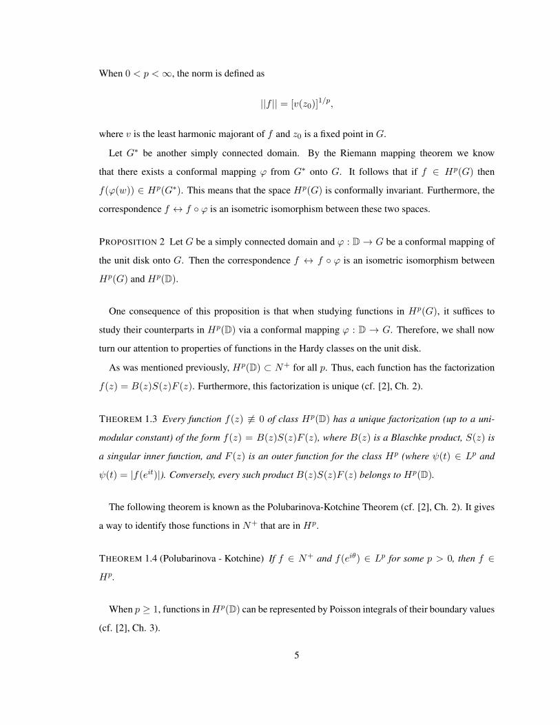
Thus, if all of the boundary curves of G are real-analytic, then Hp(G) = Ep(G) as sets. The
following example illustrates how the geometry of the domain determines the relationship between
the sets of Hp and Ep.
EXAMPLE 1 Let G be a simply connected domain bounded by a curve that is analytic except at
the point z0, where there is a corner with interior angle α. Let 0 < p < ∞. If 0 < α < π, then
Ep(G) ( Hp(G), and if π < α < 2π then Hp(G) ( Ep(G).
To see this, let us first assume that 0 < α < π. Without loss of generality let z0 = 0. Applying
the mapping
g(z) = zπ/α
to G produces an angle of π at 0. Since
g′(z) =π
αzπ/α−1
and since π/α− 1 > 0, g′(z)→ 0 as z → 0. This implies that
[g−1]′(ζ) =1
g′(g−1(ζ))→∞ as g−1(ζ)→ 0.
Let h : D→ g(G) be a conformal mapping of the unit disk onto g(G). Then
ϕ = g−1 h : D→ G
is a conformal mapping of the unit disk onto G. Assume that ϕ(1) = 0. Since ϕ′(w) → ∞ as
w → 1, then by Theorem 1.9, Ep(G) 6= Hp(G). Let f ∈ Ep(G). Then
F = f(ϕ)[ϕ′]1/p ∈ Hp(D).
8

Since 1ϕ′ ∈ H∞(D), we have
f(ϕ) =F
(ϕ′)1/p∈ Hp(D).
This implies that f ∈ Hp(G).
Next, assume that 0 < α < 2π. Let g(z) be defined as above. Then πα − 1 < 0, and g′(z)→∞
as z → 0. This implies that
[g−1]′(ζ)→ 0 as g−1(ζ)→ 0.
Let ϕ also be as defined above. Then ϕ′(w) → 0 as w → 1, so Hp(G) 6= Ep(G). Now if
f ∈ Hp(G), then f(ϕ) ∈ Hp(D). Since ϕ′ ∈ H∞(D), we have
f(ϕ)[ϕ′]1/p ∈ Hp(D).
Therefore, f ∈ Ep(G), as desired.
Functions in Smirnov classes possess boundary properties similar to functions in Hardy classes.
Functions in the Smirnov class Ep(G) have non-tangential boundary values a.e. with respect to
ds. When p ≥ 1, they can also be recovered by their boundary values. In this case, the values are
obtained using the Cauchy integral (cf. [2] Ch.10).
THEOREM 1.10 Each f ∈ E1(G) has a Cauchy representation
f(z) =1
2πi
∫Γ
f(ζ)
ζ − zdζ, z ∈ G,
and the integral vanishes when z is outside Γ. Conversly, if g ∈ L1(Γ) and∫Γzng(z)dz = 0, n = 0, 1, 2, ...,
then
f(z) =1
2πi
∫Γ
g(ζ)dζ
ζ − z∈ E1(G),
and g coincides almost everywhere on Γ with the nontangential limit of f .
1.4 Smirnov domains
The example in the previous section illustrates how the geometry of the domain determines the
classes of Smirnov and Hardy functions that exist on the domain. Simply connected domains can
be either so-called Smirnov or non-Smirnov domains, depending on the domain.
9

Let G be a simply connected domain with Jordan rectifiable boundary Γ, let D be the unit disk,
and let ϕ(w) be a conformal mapping of D onto G. Since Γ is rectifiable, then by Theorem 1.6,
ϕ′ ∈ H1 and ϕ′(w) 6= 0. This implies that ϕ′(w) = S(w)F (w) where S is a singular inner function
and F is an outer function. Note that ϕ′ is an outer function when S(w) ≡ 1.
DEFINITION 1.4.1 G is called a Smirnov domain if ϕ′(w) is an outer function.
Since ϕ′ ∈ H1(D) ⊂ N , Corollary 1.0.2 implies that if log(ϕ′) ∈ H1(D), then G is Smirnov.
Now log(ϕ′) = log|ϕ′| + i arg(ϕ′), and log(ϕ′) ∈ H1(D) is equivalent to log |ϕ′| ∈ h1(D) and
arg(ϕ′) ∈ h1(D). (A harmonic function u(z) is said to be of class h1(D) if the integral means of
the absolute value of u(z) over concentric circles tending to the boundary are bounded.) But since
G has a rectifiable boundary,
∫∂Dlog+|ϕ′(w)|ds ≤
∫∂D|ϕ′(w)|ds ≤ C.
This is equivalent to log |ϕ′| ∈ h1(D) so, actually, a necessary and sufficient condition for G to
be Smirnov is that arg(ϕ′) ∈ h1(D). In particular, if ϕ′ is bounded either from above or below then
G is said to be a Smirnov domain. This means that the boundary of G can either spiral in or out at
a point but not both.
One may ask if a bounded domain being Smirnov implies that its complement is also Smirnov.
In [9], Jones and S. K. Smirnov found that the answer to this question is in general “no”. Moreover,
when ϕ′ is a singular inner function, the complement of a non-Smirnov domain that is bounded by
Γ is Smirnov.
In the next chapter we will explore the boundary characteristics of simply connected Smirnov
domains that allow analytic functions with real boundary values in Smirnov classes Ep.
10

Chapter 2
Simply connected Smirnov domains
2.1 S. Ya. Khavinson’s Example
Since Hp(G) functions can be recovered from their boundary values via harmonic measure, any
f ∈ Hp(G) with real boundary values is real-valued inside G and hence must be a constant. Un-
like functions in the Hardy classes, it is not always true that functions in the Smirnov classes are
constants when their boundary values are real. In [10] it was shown that if G is a non-Smirnov
domain with Jordan rectifiable boundary, then there do exist functions in Smirnov classes Ep(G)
for 0 < p <∞ that are bounded a.e on Γ and possess real boundary values.
THEOREM 2.1 Let G be a simply-connected domain with a rectifiable Jordan boundary. If G is
a non-Smirnov domain, then there exists a non-constant function f(z) ∈ E1(G) such that 0 ≤
f(z) ≤ 1 a.e. on Γ.
COROLLARY 2.0.3 Let G be the same as in Theorem 2.1. Then, for each p such that 0 < p < ∞
there exists a non-constant function f(z) ∈ Ep(G) such that 0 ≤ f(z) ≤ 1 a.e. on Γ.
Furthermore, in [10] it is shown that if G is Smirnov and f(z) ∈ E1(G) is real-valued and
bounded on Γ then f(z) ≡ const. However, when the condition of boundedness is removed, an
example by S. Ya. Khavinson [10] reveals that for a certain cardioid, a Smirnov domain, the function
f(z) = F (ϕ−1(z)) where F (w) = i1+w1−w and ϕ(w) = (1−w)2 is the conformal map from the unit
disk to the cardioid (shown below), furnishes a non-trivial E1 function with real boundary values.
If we investigate this function, we notice that f(z) has a pole of order 1 at the point zero on the
boundary of the cardioid. The mapping 1+w1−w is the Mobius transformation that takes the unit disk
to the right half plane. It follows then that F (w) = i1+w1−w is the mapping of the unit disk to the
upper half plane, so it is easy to see that f(z) has real boundary values on the cardioid. Theorem 1.7
11

Figure 1.: Cardioid
states that if f(z) is of Smirnov class E1 in the cardioid then the integrals of the modulus of f over
the images of the circles |w| = r will remain bounded as r tends to 1. Looking at an image of the
modulus of f over the cardioid this is not immediately clear. The image below shows the modulus
of f and the images under ϕ of the circles of radius 1/4, 1/2, 3/4, and 1.
Figure 2.: E1 function on the Cardioid
We know that by Theorem 1.8 that f is in E1 if and only if (f ϕ)ϕ′ is in H1. On inspection of
the graph of the modulus of this function it is clear that this must be true. Below we see a graph of
the modulus of (f ϕ)ϕ′ with the images of the circles of radius 1/4, 1/2, 3/4, and 1.
12

Figure 3.: H1 function on the Circle
In fact, the example works for all p such that 0 < p < 2. To see that this is true, recall that
Theorem 1.8 states that f(ϕ(w))[ϕ′(w)]1/p ∈ Hp(D) if f(z) ∈ Ep(G). Since
f(ϕ(w))[ϕ′(w)]1/p = i1 + w
1− w· [−2(1− w)]1/p = −2i(1 + w)(1− w)1/p−1
Then f(z) ∈ Ep(G) if p(1/p− 1) > −1 or p < 2.
S. Ya. Khavinson’s example leads us to believe that the existence of Ep functions with real
boundary values is dependent upon the local geometry of the domain. With this example in mind,
one might ask the following questions: What are the boundary characteristics of a Smirnov domain
that will admit functions with real boundary values in the Smirnov classes Ep? For what values of
p will these functions exist? What can be said about analytic functions with real boundary values in
the Smirnov classes Ep on finitely connected Smirnov domains? Let us note here that it is desirable
to find analytic functions with real boundary values in classes Ep for p ≥ 1 as it is these classes of
functions that have the property that they can be recovered inside a domain by use of their boundary
values.
2.2 Domains with interior angles less than π
After considering S. Ya. Khavinson’s example, I first would like to consider a simply connected
domain whose boundary is nice, say real analytic, except at one point were the boundary has an
outward pointing corner. Let us suppose that the interior of this corner has an angle less than π. It
happens that these functions do not admit non-constant analytic functions of Smirnov class Ep for
13

Figure 4.: Domains with interior angles less than π.
p ≥ 1 with real boundary values on such domains [4].
THEOREM 2.2 Let G be a domain bounded by a curve that is real analytic except at the point z0
where it has a corner with interior angle α. If 0 ≤ α ≤ π, then for all p ≥ 1 every f(z) ∈ Ep(G)
with real boundary values is a constant.
Note. The angle α = 0 corresponds to an outward cusp. The angle α = π corresponds to Γ being
smooth and was discussed above.
Proof. Let 0 < α < π and suppose that there exists an f(z) ∈ E1(G) with real boundary values
a.e. Without loss of generality we may assume that ϕ(1) = z0. According to [18], Ch. 3, Sec. 4,
ϕ′(w) = (1− w)απ−1g(w), (2.1)
where g(w) is bounded away from 0 and∞ in D. Then by Theorem 1.8,
f(ϕ(w))ϕ′(w) = f(ϕ(w))(1− w)απ−1g(w) ∈ H1(D).
Since απ − 1 < 0, multiplying by a bounded, analytic function in D, (1− w)1−α
π , we conclude that
f(ϕ(w)) ∈ H1(D). Since f(ϕ(w)) can be represented by the Poisson integral in D and has real
boundary values then f(ϕ(w)) is real-valued in D and hence is a constant. For the case when α = 0
we need a result from [18] Ch. 11, Sec. 5, which states that
limw→1|ϕ(w)− ϕ(1)| =
πa + o(1)
log 1|w−1|
, (2.2)
14
where a > 0, is a constant. This means that
|ϕ′(1)| = limw→1
|ϕ(w)− ϕ(1)||w − 1|
=∞. (2.3)
So if f(ϕ(w))ϕ′(w) ∈ H1(D) then f(ϕ(w)) ∈ H1(D) which implies as before, that f(ϕ(w)) ≡
const.
To show that for all p such that 0 < p < 1 there exists in such G a f(z) ∈ Ep(G) with real
boundary values, consider the function F (w) = i1−w1+w which maps the unit disk onto the upper half
plane. Suppose that 0 < α < π. Then f(z) = F (ϕ−1(z)) ∈ Ep(G) for 0 < p < 1. Indeed by
Theorem 1.8 and (2.1) we have:
f(ϕ(w))[ϕ′(w)]1p = F (w)(1− w)
(απ−1) 1
p g1p (w) = i
(1− w)1+ α
πp− 1p
(1 + w)g
1p (w).
So f(ϕ(w))[ϕ′(w)]1p ∈ Hp(D) for 0 < p < 1, since p (1 + α
πp −1p) = p + α
π − 1 > −1. When
α = 0 we use (2.2) and (2.3) to see that
|f(ϕ(w))|p|ϕ′(w)| =∣∣∣∣i1− w1 + w
∣∣∣∣p |ϕ′(w)| ≈(πa + o(1))|1− w|p−1
|1 + w|p∣∣∣log 1
|w−1|
∣∣∣ ,which is integrable on T for 0 < p < 1, while obviously is in classN+(D). Hence the Polubarinova-
Kotchine Theorem applies and f(z) ∈ Ep(G).
For α = π, Γ is smooth and the existence of a non-trivial f(z) ∈⋂p<1
Hp(G) with real boundary
values is obvious. For example, in D it suffices to take F (w) itself.
While this type of domain does admit non-constant analytic functions of classEp with real bound-
ary values, none of these functions can be recovered by their boundary values via the Cauchy integral
since p < 1.
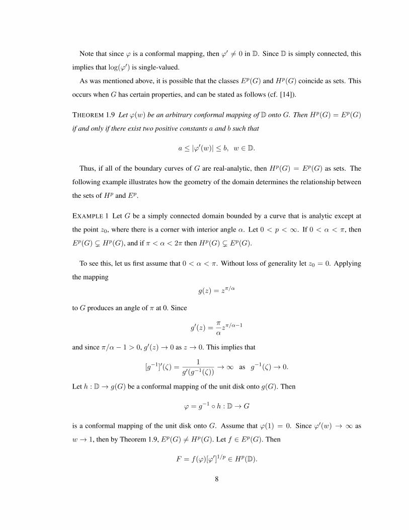
2.3 Domains with interior angle greater than π
Now we shall examine the case when G is a simply connected domain that has a real analytic
boundary except at one point where there is an inward pointing corner with interior angle greater
than π. As we shall see this is an interesting case when nontrivial functions with real boundary
values can be found in Ep for p ≥ 1 [4].
15

Figure 5.: Domains with interior angles greater than π.
THEOREM 2.3 Let G be a domain bounded by a curve that is real analytic except at the point z0
where it has a corner with interior angle α. If π < α ≤ 2π then for all p ≥ απ every f(z) ∈ Ep(G)
with real boundary values is a constant. If p < απ then there does exist a non-constant function in
Ep(G) with real boundary values.
Note. The angle α = 2π corresponds to Γ having an inward cusp, e.g. a cardioid as in [10]. Thus
G obtained from D via the conformal map ϕ(w) = (1 − w)2 doesn’t have a non-constant E2(G)
function with real boundary values.
Proof. Suppose that there exists such f(z) ∈ Eαπ (G). Without loss of generality assume that
ϕ(1) = z0. Then by the Keldysh-Laurentiev theorem and (2.1)
h(w) := f(ϕ(w))[ϕ′(w)]πα = f(ϕ(w))(1− w)1− π
α gπα (w) ∈ H
απ (D).
Set
h0(w) :=h(w)(1− w)
πα
gπα (w)
= f(ϕ(w))(1− w) ∈ Hαπ (D).
Thenh1(w)
w:= h0(w)(1− w) = f(ϕ(w))|1− w|2 (2.4)
16

has real boundary values on T. Now h1(w) ∈ Hαπ (D) ⊂ H1(D) since α
π ≥ 1 and by the general-
ized Schwarz reflection principle, h1(w)w extends across T to the Riemann sphere. So it is a rational
function with a pole of order 1 at the origin and infinity.
Case 1. Suppose h1(w) does not have any poles on T. Then
h1(w)
w= C
(w − β)(1− βw)
wwhere β ∈ D and C ∈ R. (2.5)
Since f(ϕ(w))(1−w) ∈ Hαπ (D) ⊂ H1(D), f(ϕ(w)), which is also a rational function since h0(w)
and h1(w) are, cannot have a pole of order greater than 1. Then from (2.5) it follows at once that
β = 1 sinceh1(w)
w=f(ϕ(w)(1− w)(w − 1)
w,
but then f(ϕ(w)) ≡ C, hence f(z) is itself a constant.
Case 2. Suppose h1(w) does have poles on T. From (2.4) it follows that it can only be at w = 1
and of order 1 (it is in H1(D)!) Thus,
h1(w)
w= C
(w − β1)(w − β2)(1− β2w)
(1− w)w, where β1 ∈ T , β2 ∈ D
and Cw − β1
1− w∈ R on T.
We claim that β1 = −1 and C is purely imaginary. Let w = a+ bi ∈ T and β1 = c+ di. Then
C(w − β1)
(1− w)= C
(a+ bi− c− di)(1− a)− bi
= C((a− c) + (b− d)i)
(1− a)− bi((1− a) + bi)
((1− a) + bi)(2.6)
= C[(a− c)(1− a) + (1− a)(b− d)i+ (a− c)bi− (b− d)b]
(1− a)2 + b2.
Since (2.6) is real-valued, then either C is real and(1− a)(b− d) + (a− c)b = 0 or C is purely
imaginary and (a− c)(1− a)− (b− d)b = 0. In the first instance d = 0 and c = 1 which implies
that we have Case 1. In the second instance a− a2 − c+ ca− b2 + bd = 0 and since a2 + b2 = 1
then a− c+ ca− 1 + bd = 0 which implies that c = −1 and d = 0. Therefore β1 = −1 and C is
purely imaginary. Thus
h1(w)
w= it
(w + 1)(w − β2)(1− β2w)
(1− w)w=f(ϕ(w))(1− w)(w − 1)
w,
17

where t ∈ R. Therefore, β2 = 1 and
f(ϕ(w)) = itw + 1
1− w,
but,
f(ϕ(w))(1− w)1− πα g
πα (w) = it
w + 1
(1− w)πα
gπα (w) /∈ H
απ (D).
So Case 2 cannot occur and the proof is complete.
For α such that π < α ≤ 2π an argument similar to S. Ya. Khavinson’s in [10] shows that for all
p such that 0 < p < απ there exists a non-constant f(z) ∈ Ep(G) with real boundary values. Let
F (w) = i1+w1−w . F (w) maps the unit disk onto the upper half plane. Then f(z) = F (ϕ−1(z)) ∈
Ep(G). This follows from Theorem 1.8 and (2.1) since
f(ϕ(w))[ϕ′(w)]1p = F (w)(1− w)
(απ−1) 1
p g1p (w)
= i(1 + w)(1− w)απp− 1p−1g
1p (w)
and f(ϕ(w))[ϕ′(w)]1p ∈ Hp(D) when p ( απp −
1p − 1) > −1 or p < α
π .
Interestingly, the proof of Theorem 2.3 also shows that the transplanted mappings F (w) of D
onto a half plane, e.g. f(z) := F (ϕ−1(z)), where F (w) = i1+w1−w are essentially the only examples
of functions in Ep(G), p ≥ 1 with real boundary values. Thus S. Ya. Khavinson’s construction in
[10] is, in this sense, unique.
If a domain is bounded by an analytic curve with finitely many corners (or, cusps) it follows that
the existence of an Ep function with real boundary values is dependent upon the corner with the
smallest interior angle.
18

Chapter 3
Finitely connected domains
3.1 Some background on n-connected domains
LetG be a finitely connected domain in the complex plane with boundary Γ =⋃nj=1 γj . A bounded,
finitely connected domain K is called a circular domain if all of the boundary components of K are
all circles. The following theorem is due to Koebe and its proof can be found in [7], Ch. 5.
THEOREM 3.1 Every n-connected Jordan domain G can be univalently mapped onto a circular
domain K.
When a conformal mapping from a circular domain K onto an n-connected domain G takes
the outer boundary circle of K to the outer boundary curve of G, then the mapping preserves the
orientation of all of the boundary curves. This implies that the logarithm of the derivative of the
conformal mapping is single-valued on K. Namely, the following holds.
PROPOSITION 3 Let ϕ : K → G be the conformal map of K onto G. Assume that the outer circle
of K is mapped onto the outer boundary curve of Γ := ∂G. Then log(ϕ′) has a single-valued
branch in K.
Proof. Let w = ϕ(z). Then, the tangent vector to Γ is dw = ϕ′(z)dz.
Since
2π = ∆ln arg(dw) = ∆γn arg(ϕ′) + ∆γnarg(dz)
and
∆γn arg(dz) = 2π,
then ∆γn arg(ϕ′) = 0. Similarly,
−2π = ∆lj arg(dw) = ∆γj arg(ϕ′) + ∆γj arg(dz)
19

and
∆γj arg(dz) = −2π for j = 1, ..., n− 1.
This implies that ∆γj arg(ϕ′) = 0 for all j = 1, ..., n. Therefore, log(ϕ′) is single-valued on K.
In Section 1.1 the harmonic measure for a Dirichlet region was defined. One can also define the
harmonic measures ωj of γj , j = 1, ..., n on ∂G. These are harmonic functions in G such that
ωj |γj ≡ 1 and ωj |γk ≡ 0 when j 6= k.
If u(z) is a harmonic function in G, then its harmonic conjugate v(z) may be multivalued in G.
Suppose that u(z) can be represented by the Green-Stieltjes integral of a Borel measure µ supported
on Γ. This means that
u(z) =1
2π
∫Γ
∂g(ζ, z)
∂nζdµ(ζ),
where ∂∂nζ
is the inner normal derivative at the point ζ and g(ζ, z) is the Green funtion of G with
pole at z. Then we can compute the period of v(z) around γj , j = 1, ..., n (cf. [12]) as
∆γjv = −∫
Γ
∂ωj∂n
(ζ)dµ(ζ).
Lemma 1 in [12] provides a way to eliminate the periods of v and produce an analytic function
by modifying µ. More precisely,
LEMMA 3.1 Let µ > 0 (or µ < 0) be a Borel measure on Γ such that µ(γj) 6= 0, j = 1, ..., n− 1.
Then, for arbitrary real numbers Λ1, ...,Λn−1 there exists a unique vector (λ1, ..., λn−1) ∈ Rn−1
such that Λ1, ...,Λn−1 are the periods around γ1, ..., γn−1 respectively of the function conjugate to
u(z) =1
2π
∫Γ
∂g(ζ, z)
∂nζdµ(ζ),
where µ|γn ≡ µ|γn , µ|γj ≡ λjµ|γj , j = 1, ..., n− 1.
The proof of the lemma ([12]) reduces to showing that the system of linear equations
−n−1∑j=1
λj
∫γj
∂ωi(ζ)
∂nζdµ(ζ) = Λi +
∫γn
∂ωi(ζ)
∂nζdµ(ζ) , i = 1, ..., n− 1 , λj ∈ R, (3.1)
always has a unique solution.
20

Suppose G is an n-connected domain and dµ is a measure on ∂G that is defined as the sum of
point masses. If u is the harmonic function represented by the Green-Stieltjes integral with measure
dµ then it is often possible to modify the measure so that the resulting harmonic function has a
single-valued conjugate. Hence, one can construct an analytic function on G that is real-valued
almost everywhere on ∂G. The existence of such functions will be necessary for two theorems that
will be presented later in this thesis. The next proposition is from [5].
PROPOSITION 4 Let u(z) be a harmonic function in G such that u(z) is represented by the Green-
Stieltjes integral with dµ =∑m
j=1 δζj , where δζj is the unit point mass at ζj . If m ≥ n then there
exist real numbers λ1, ..., λm that are not all equal to zero such that the function
u(z) = λ1∂g(z, ζ1)
∂nζ1+ ...+ λm
∂g(z, ζm)
∂nζm
has a single valued conjugate.
Proof. Consider the matrix A associated with the system of equations (3.1). Namely,
A = ||aij ||, where aij =∂ωi(ζj)
∂nζj. (3.2)
Let ~λ = (λ1, ..., λm) 6= 0. Then u will have a single-valued conjugate if A~λ = 0. Since A : Rm →
Rn−1 is a linear map given by the matrix A, it suffices to show that ker(A) 6= 0. Since m =
dim(ker(A)) + dim(rank(A)) and dim(rank(A)) ≤ n − 1 then dim(ker(A)) ≥ 1. Therefore
ker(A) 6= 0.
The following example illustrates a case when rank(A) = n− 1.
EXAMPLE 2 If m ≥ n and there exists j where 1 ≤ j ≤ m such that ∃ζj ∈ γi for each i = 1, ..., n
then there exist λ1, ..., λm not all equal to zero such that u has a single-valued conjugate. Without
loss of generality we may assume that ζ1 ∈ γ1, ..., ζn−1 ∈ γn−1. Then by Lemma 1 in [12] the
minor of the matrix A in (3.2) formed by the first (n − 1) columns and first (n − 1) rows has rank
(n− 1) and therefore, A~λ = 0 has a non-zero solution.
The converse of Proposition 4 is not true. It can happen that m < n and yet u has a single-valued
conjugate.
21

Figure 6.: S. Ya. Khavinson’s example
EXAMPLE 3 (S. Ya. Khavinson, [13]): LetG be the domain bounded by the circles γ1 = z : |z| =
1, γ2 = z : |z + 1/2| = 1/4, and γ3 = z : |z − 1/2| = 1/4. Let ζ1 = −1/2 + 1/4i and
ζ2 = −1/2 − 1/4i. Then ζ1, ζ2 ⊂ γ2 and ζ1 is symmetric to ζ2 with respect to the horizontal
diameters of γi, i = 1, 2, 3. Thus by symmetry,
∂ωi(ζ1)
∂nζ1=∂ωi(ζ2)
∂nζ2,
for i = 1, 2. So the two rows of A are linearly dependent, and the equations
λ1∂ωi(ζ1)
∂nζ1+ λ2
∂ωi(ζ2)
∂nζ2= 0, i = 1, 2
have non-zero solutions λ1 = −λ2.
3.2 The Hardy and Smirnov classes revisited
The definition of the Hardy classes stays the same when G is a finitely connected domain. That
is, Hp(G) for 0 < p < ∞ is the space of analytic functions f such that the subharmonic function
|f(z)|p has a harmonic majorant in G. The definition of the norm of a function in Hp(G) stays the
same as in Section 1.2 however, the norm is only a true norm for all p ≥ 1.
Before going further, let us recall a theorem from [7] Chapter VI, sec.1 that basically states that
if a domain G possesses more than two boundary points then there exists an analytic function T (w)
that is locally univalent and maps the unit disk onto G. T (w) is called the uniformization map of
22

G. Let Σ be the group of deck transformations of D associated with T (cf. [6] Ch. 2, Sec. 2). This
means that if g ∈ Σ then g : D → D is a Mobius automorphism of the unit disk onto itself and
T (g(w)) ≡ T (w). Given a point z0 ∈ G, T can be chosen so that then T (0) = z0 and T ′(0) > 0.
Given these normalizations, T is unique.
We now state the following theorem from [2], Thm. 10.11.
THEOREM 3.2 The mapping
f(z)→ F (w) = f(T (w))
is an isometric isomorphism of Hp(G) onto the subspace of Hp(D) invariant under Σ.
This theorem implies that if G is finitely connected then some properties of functions in Hp(G)
can be investigated using their counterparts in Hp in the unit disk. The proof of the following
theorem follows from the Green formula and can be found in [2], Ch. 10, Sec. 5, also cf. [14], [15]
and references therein.
THEOREM 3.3 Let G be a finitely connected domain with Jordan boundary curves γ1, ..., γn. For
each j = 1, ..., n let Gj be the simply connected domain with boundary γj which contains G. Then
every f ∈ Hp(G) can be represented in the form
f(z) = f1(z) + f2(z) + ...+ fn(z),
where fj ∈ Hp(Gj) for j = 1, ..., n.
Note that if in the above theorem fj(∞) = 0 for j = 1, ..., n − 1, then the fj are all unique. It
follows from this theorem and Theorem 1.5 that a function f ∈ Hp(G) must have non-tangential
boundary values a.e. with respect to harmonic measure, ωa, on ∂G. That is ωa = ω(G,Γ, a) where
a ∈ G is fixed. It is also true that an analytic function in the Hardy class Hp, p ≥ 1, of a finitely
connected domain can be recovered by its boundary values just like in the simply connected case.
The following theorem is from [14].
THEOREM 3.4 Each f ∈ Hp(G) for 1 ≤ p ≤ ∞ has boundary values f∗ almost everywhere with
respect to dω on Γ and f∗ ∈ Lp(Γ, dω). Furthermore,
f(z) =1
2πi
∫Γf∗(ζ)dωz(ζ), z ∈ G.
23

We can also speak of a factorization for functions in Hardy classes in finitely connected domains.
First we need the notion of a Green-Schwarz kernel in G (cf. [1], [11], and [13]).
THEOREM 3.5 There exists a unique function P(z, ζ) continuous on G × Γ and satisfying the fol-
lowing properties:
1. If ζ ∈ Γ is fixed, then P(z, ζ) is single-valued and analytic in G.
2. If z ∈ G is fixed, then ∫γj
P(z, ζ)dωa = 0 j = 1, .., n− 1,∫γn
P(z, ζ)dωa = 1.
3. If f(z) = u(z) + iv(z) is a single-valued analytic function in G and u(z) is continuous in G,
then
f(z) =
∫ΓP(z, ζ)u(ζ)dωa + iv(a).
P(z, ζ) is called the Green-Schwarz kernel in G.
Let a ∈ G and following [1] and [11], define the function
B(z, a) = (z − a)exp
(−∫
ΓP(z, ζ)ln|ζ − a|dω
).
Note that when a ∈ G, the above function maps G conformally onto the unit disk with slits along
circular arcs centered at the origin. When a ∈ Γ, B(z, a) maps G conformally onto an annulus with
slits along n − 2 circular arcs centered at the origin (cf. [1]). This also means that |B(z, a)| is a
constant on each boundary curve of G.
For the next theorem (cf. [11] and references there) let us recall the following notation. g(a, z) is
the Green function of G with pole at a and ∂G = Γ =⋃n
1 γj . Let Gj be the domain bounded by γj
and containing G, ωj(z) be the harmonic measure of γj , and gj(a, z) be the Green function of Gj .
THEOREM 3.6 Let f(z) be a single-valued analytic function in G. Let zk∞1 be the sequence of
its zeros in G. The following statements are equivalent:
1. ln |f(z)| has a harmonic majorant in G.
2. The series∑∞
1 g(zk, z) converges uniformly on compact subsets of G \ zk∞1 .
24

3. Let zjk∞1 , j = 1, ...n, be the subsequences of zk∞1 such that all cluster points of zjk
belong to γj; zk∞1 =⋃nj=1z
jk∞k=1, zik∞k=1 ∩ z
jk∞k=1 = ∅ when i 6= j. Then the series∑∞
k=1 gj(zjk, z), j = 1, ..., n, converge uniformly on compact subsets of Gj \ zjk
∞k=1.
4. The series∑∞
k=1 |ωi(zjk) − δij |, i = 1, ..., n, j = 1, ..., n, converge. (δij is the Kronecker
symbol.)
If Γ =⋃n
1 γj is analytic and ζj denotes the closest point to zj on Γ, then (1) through (4) are
equivalent to the following:∞∑j=1
|zj − ζj | < +∞.
Let ϕ : K → G be the conformal map of the circular domainK ontoG. Assume that γ1, ..., γn−1
lie inside γn and introduce the periods of the conjugates of the harmonic functions ωk
πkj =
∫γ′j
∂ωk∂s
ds = −∫γ′j
∂ωk∂n
ds,
j, k = 1, ..., n− 1, where γ′j is an analytic curve in G homologous to γj . The matrix (πkj)n−11 is in-
vertible (it follows from [12] Lemma 1; also see [1]), which implies that (qkj)n−11 =
((πkj)
n−11
)−1
is well defined. The following theorem is from [11] and its proof there is similar to that in [1].
THEOREM 3.7 Let zk∞k=1 satisfy (1)-(4) of Theorem 3.6. Define wjk = ϕ−1(zjk) and let tjk be the
point closest to wjk on ∂K. Let ζjk = ϕ(tjk). Then the product
B0(z) =
n∏j=1
∞∏k=1
B(z, zjk)
B(z, ζjk),
converges absolutely and uniformly on compact subsets of G. B0(z) = 0 if and only if z ∈ zk∞1 .
Moreover, if the sequence Gi∞i=1 is a sequence of domains such that Gi ⊂ Gi+1 and⋃∞i=1G
i =
G, then (letting Γi = ∂Gi =⋃nk=1 γ
ik)
limi→∞
∫γ′k
| ln |B0(z)| − Ck|dωi(E, a,Gi) = 0
where
Ck =
∞∑i=1
n∑l=1
n−1∑j=1
qjk(δjl − ωj(zli)), k = 1, ..., n− 1; Cn = 0.
Finally, |B0(ζ)||γk = exp(Ck) a.e. with respect to dω, k = 1, ..., n.
25

B0(z) is called the generalized Blaschke product.
We now present the factorization theorem for analytic functions in the Hardy classes of finitely
connected domains as stated in [11] for Jordan domains, and [1] for domains with analytic bound-
aries.
THEOREM 3.8 f(z) ∈ Hp(G) if and only if
f(z) = Q(z)B0(z)exp
(∫ΓP(z, ζ)dµ(ζ)
), (3.3)
where the zeros of B0 correspond to the zeros of f(z); dµ = ln|f(ζ)|dω + dν and dν ≤ 0 is
singular with respect to dω;
Q(z) = exp
(n−1∑
1
λjwj(z)
), wj(z) = ωj(z) + iωj(z),
where the λj are real numbers such that the numbers (1/2π)∆γkarg(Q(z)) are integers. Moreover,∫Γ|f(ζ)|pdω(E, a,G) ≤ const < +∞.
The definition of functions in the Smirnov classes in G is very similar to that of the simply
connected case (cf.[2], Ch.10). A function f analytic in G is said to belong to the class Ep(G) if
there is a sequence of domains Ωj in G with boundaries Γj that consist of a finite number of
rectifiable curves, such that Ωj eventually contains each compact subset of G, and
limj→∞
∫Γj
|f(z)|p|dz| <∞.
S. Ya. Khavinson and G. Tumarkin have extended the Keldysh-Lavrentiev theorem (theorem 1.8)
to finitely connected domains [15].
THEOREM 3.9 Let ϕ : K → G be the conformal mapping of the circular domain K onto G. Then
f(z) ∈ Ep(G) if and only if f(ϕ(w))[ϕ′(w)]1/p ∈ Hp(K).
(Note that [ϕ′(w)]1/p is single-valued in view of Proposition 3.)
Let ψ : G→ K be the conformal map from G onto K and assume that Γ is rectifiable. It follows
from Theorem 3.9 that ψ′(z) ∈ E1(G). Also, since ψ′(z) 6= 0 in G, then ψ′(z) can be written as
ψ′(z) = exp
∫ΓP(z, ζ)dµ0
,
26

where dµ0 = ln |ψ′(ζ)|dω + dν0 and dν0 is a singular measure [11]. Moreover, dν0 ≥ 0 cf. [11].
Functions in Smirnov classes on finitely connected domains with rectifiable boundaries also admit
a factorization that is similar to those of Hp function in finitely connected domains. The next
theorem is due to D. Khavinson ([11], Thm.4.6).
THEOREM 3.10 f(z) ∈ Ep(G), p > 0, if and only if (3.3) holds with dµ = ln |f(ζ)|dω + dν,
where dν is singular, dν ≤ 1pdν0 and
∫Γ |f(ζ)|pds < +∞.
If we further require that all of the boundary curves ofG are rectifiable, then a theorem analogous
to Theorem 1.10 can be proven for functions of class Ep(G) . This means that if f ∈ Ep(G) then f
has non-tangential boundary values a.e., so if p ≥ 1, then f can be recovered inG from its boundary
values by a Cauchy integral over Γ (cf. [2], Ch. 10).
Remark. The theorems presented here are restricted to n-connected domains. However, the
Smirnov classes can also be defined on infinitely connected domains. That is, domains that have an
infinite number of boundary components. Let us note the following theorem from [19].
THEOREM 3.11 Let G be a domain with countably many boundary components. Then G is confor-
mally equivalent to a domain bounded by analytic Jordan curves and points.
The implication of this theorem is that on such domains the Keldysh- Lavrentiev theorem holds
and hence the Smirnov classes are linear spaces. Whether this stays true for Smirnov classes on
arbitrary infinitely connected domains with uncountably many boundary components is an open
question.
3.3 Finitely connected Smirnov domains
Definition 1.4.1 also applies to n-connected domains (cf. [15]). That is, G is called a Smirnov
domain if the conformal mapping ϕ : K → G of an n-connected circular domain K onto G is an
outer function. Let l1,..., ln be the circular boundary curves of K. Let Ki be the simply connected
domain bounded by li containing K and Gi be the simply connected domain bounded by γi and
containing G. Each function ϕi : Ki → Gi, i = 1,...,n will denote the conformal mapping of Ki
onto Gi. S. Ya. Khavinson and G. Tumarkin have shown that G being Smirnov is also equivalent to
ϕi(w) being outer functions for all i = 1,...,n ([15]).
27

The following useful observation from [15] connects the growth/decay of the conformal mapping
ϕ : K → G with that for ϕi, i = 1, ..., n, near respective boundary components.
LEMMA 3.2 There exist constants c1 and c2 such that the inequalities
0 < c1 ≤∣∣∣∣ ϕ′(w)
ϕi′(w)
∣∣∣∣ ≤ c2 <∞
holds near li for all i = 1, ..., n.
The proof follows at once after one observes that ϕ ϕ−1i preserves li, is one to one near it, and
hence extends analytically across li. We emphasize here that in Lemma 3.2 the boundary of G is
assumed to be merely Jordan and rectifiable.
It is convenient to single out a subclass of non-Smirnov domains that are called “completely
non-Smirnov” (cf. [10]).
DEFINITION 3.3.1 We shall callG a “completely non-Smirnov” domain if and only if all the simply
connected domains Gi, i = 1, ..., n do not belong to the Smirnov class.
These domains do admit functions in Smirnov classes Ep(G) for 0 < p <∞ which are bounded
a.e on Γ and possess real boundary values. The following two theorems are from [10].
THEOREM 3.12 Let G be a completely non-Smirnov domain. Then there exists a non-constant
function f(z) ∈ E1(G) such that 0 ≤ f(z) ≤ 1 a.e. on Γ.
THEOREM 3.13 LetG be a completely non-Smirnov domain. Then, for each p such that 0 < p <∞
there exists a non-constant function f(z) ∈ Ep(G) such that 0 ≤ f(z) ≤ 1 a.e. on Γ.
At this point, we have resolved the problem of the existence of non-constant analytic functions of
the Smirnov classes with real boundary values for simply connected Smirnov domains. D. Khavin-
son has discussed the case when the domain under consideration is simply connected and non-
Smirnov. He also investigated the case when the domain is finitely connected and completely non-
Smirnov. In the next chapter, I will consider the case when a given domain is a finitely connected
Smirnov domain.
28

Chapter 4
Finitely connected Smirnov domains
4.1 The representation of analytic functions with certain boundary properties
Before the main theorems of this thesis are presented, we first need to investigate the structure of
analytic functions in simply connected domains bounded by a real analytic curve that have real
boundary values except at one point where the function is unbounded. The following lemma (cf.
[5]) addresses the simple case when the domain is the unit disk. The corollary (cf. [5]) that follows
shows that a similar result is obtained for arbitrary simply connected domains.
Let D be the unit disk and T = ∂D. Let Ω be a simply connected domain in the complex plane
bounded by a real analytic curve. We shall define RΩ(z, ζ) to be the Schwarz kernel of Ω. This
means that
RΩ(z, ζ) =1
2π
∂P (z, ζ)
∂nζ, where P (z, ζ) = g(z, ζ) + ig(z, ζ),
z ∈ Ω, ζ ∈ ∂Ω, ∂∂nζ
is the inner normal derivative, and g and g are respectfully the Green function of
Ω with pole at z and its harmonic conjugate. For example, when Ω = D then RD(z, ζ) = 12π
eiθ+zeiθ−z .
Let ∂∂τ denote the tangential derivative.
LEMMA 4.1 Suppose f = u+ iv is analytic in D, continuous in D \ 1, and v ≡ 0 on T \ 1. If
|f | = O(
1|1−z|k
)near 1, then
f(z) =
k−1∑n=0
λn∂n
∂τniRD(z, 1) + c,
where λk−1,...,λ0, c ∈ R.
Proof. We proceed by induction. Suppose k = 1. Then by the generalized Schwarz reflection
principle f extends to be analytic in C \ [1,∞). So |f(z)| = O(
1|1−z|
)in D. Consider F = f τ ,
where τ−1(z) = 1+z1−z is the conformal mapping of D onto the right half plane. Then |F (z)| = O(|z|)
29

and =F (z) = 0 on it : t ∈ R. By the Schwarz reflection principle F extends to be an entire
function. Therefore F (z) = Az +B, where A,B ∈ C. This implies that
f(z) = A1 + z
1− z+B.
Since =f(z) = 0 on T \ 1, then A = λi and λ,B ∈ R. Suppose the statement holds for some k.
Again, looking at f τ , we conclude that f is a rational function with a pole at 1 of order k. Since∣∣∣∣ ∂k∂θkRD(z, 1)
∣∣∣∣ = O
(1
|1− z|k+1
),
then λk ∈ R \ 0 can be chosen so that∣∣∣∣f(z)− λk∂k
∂θkiRD(z, 1)
∣∣∣∣ = O
(1
|1− z|j
),
where j ≤ k. Since
=(f(z)− λk
∂k
∂θkiRD(z, 1)
)= 0
on T \ 1, then
f(z)− λk∂k
∂θkiRD(z, 1) =
k−1∑n=0
λn∂n
∂τniRD(z, 1) + c,
where λk−1, ..., λ0, c ∈ R. Therefore f(z) =∑k
n=0 λn∂n
∂τn iRD(1, z) + c.
REMARK 1 If an analytic function f(z) in D has real boundary values on T \ 1 and |f(z)| =
O(
1|1−z|β
)where β ∈ R+ then |f(z)| = O
(1
|1−z|[β]
). To see that this is true note that by the gen-
eralized Schwarz reflection principle f extends to be analytic in C \ [0,∞) so |f(z)| = O(
1|1−z|β
)in D. Letting F = f τ where τ−1(z) = 1+z
1−z is the conformal mapping of D onto the right half
plane, then |F (z)| = O(|z|β) and =F (z) = 0 on it : t ∈ R. By the Schwarz reflection prin-
ciple F extends to be an entire function. Therefore, by an easy corollary of Liouville’s Theorem,
F (z) = akzk + ...+ a1z + a0, where k ≤ [β]. Thus
f(z) = ak
(1 + z
1− z
)k+ ...+ a1
(1 + z
1− z
)k−1
+ a0.
Therefore |f(z)| = O(
1|1−z|[β]
).
The following Corollary (cf. [5]) follows immediately by a simple change of variables.
30

COROLLARY 4.1.1 If f = u + iv is analytic in Ω, where Ω is a simply connected domain with
analytic boundary, v ≡ 0 on ∂Ω \ ζ, continuous in Ω \ ζ, and |f(z)| = O(
1|ζ−z|k
)near ζ,
then
f(z) =k−1∑n=0
λn∂n
∂τniRΩ(z, ζ) + c,
where λk−1,...,λ0, c ∈ R.
The next corollary (cf. [5]) shows that Lemma 4.1 and Corollary 4.1.1 are, in fact, local proper-
ties.
COROLLARY 4.1.2 Let Ω be as above. Let u be harmonic in Ω and smooth in Ω \ ζ0. If on the
arc γε ⊂ ∂Ω where ζ0 ∈ γε, u(ζ) ≡ 0 on γε \ ζ0 and |u(z)| = O(
1|ζ0−z|k
)near ζ0 then
u(z) =
∫∂Ω\γε
∂
∂nζg(z, ζ)u(ζ)ds+
k−1∑j=0
λj∂j
∂τ j
(∂
∂nζ0g(z, ζ0)
),
where λk−1,...,λ0 ∈ R.
Proof. Let
u1(z) =
∫∂Ω\γε
∂
∂nζg(z, ζ)u(ζ)ds
and let v be the harmonic conjugate of u−u1. Let f = v+ i(u−u1). Then |f | = O(
1|ζ0−z|k
)and
satisfies the hypothesis of Corollary 4.1.1. Therefore,
f(z) =
k−1∑j=0
λj∂j
∂τ jiRΩ(z, ζ0) + c,
where c, λ0,...,λk−1 ∈ R. Since < RΩ(z, ζ0) = ∂∂nζ0
g(z, ζ0),
(u− u1)(z) =k−1∑j=0
λj∂j
∂τ j
(∂
∂nζ0g(z, ζ0)
).
Therefore,
u(z) =
∫∂Ω\γε
∂
∂ng(z, ζ)u(ζ)ds+
k−1∑j=0
λj∂j
∂τ j
(∂
∂nζ0g(z, ζ0)
),
where λk−1,...,λ0 ∈ R.
REMARK 2 Note that if a harmonic function u satisfies the hypothesis of Corollary 4.1.2 with the
exception that |u(z)| = O(
1|ζ0−z|β
)near ζ0 where β ∈ R+, then |u(z)| = O
(1
|ζ0−z|[β]
). This
statement follows now from Remark 1 and the proof of Corollary 4.1.2.
31

4.2 A digression: the potential function of a fluid flow
Consider a two-dimensional incompressible fluid in a bounded simply connected domain Ω in the
complex plane. Let Φ = φ + iψ, be the fluid potential function of this system. This function
describes the nature of a steady fluid flow.
The real part of Φ, φ, is the velocity potential of the fluid flow. It usually represents the irrotational
component of the fluid potential. Its gradient, ∇φ = ~v = (u(x, y), v(x, y)), is the velocity of the
fluid. When the curl of the gradient is zero, the fluid is said to be irrotational. The divergence of the
gradient, ∇2φ = ∇ · ~v, is the divergence of the fluid flow. When Φ is analytic, then this divergence
is zero indicating that the fluid is incompressible.
The imaginary part of Φ, is known as the stream function. The level curves of ψ are the stream
lines of the fluid. The streamlines indicate the direction of travel of a component of the fluid. The
difference in value of the steam function between any two points indicates the flux of the fluid
across the curve connecting those two points. The gradient of ψ, ∇ψ = ~∗v = (−v(x, y), u(x, y))
is the force on the rotational components (vortices) of the fluid (cf. [8]). The Laplacian of ψ,
∇2ψ = ∇ × ~v = −ω is the only component of vorticity of the fluid. If Φ is analytic in a domain,
then∇2ψ = 0 and no vortices exist in the domain.
For a general reference regarding the fluid potential function we direct the reader to [16] Ch.
3, Sec. 2. A function of the type described in Lemma 4.1 and Corollary 4.1.1 corresponds to a
fluid flow in which 2k−1 sources and 2k−1 sinks of increasing strength approach each other from
opposite sides of the boundary of Ω to form “multipoles”. Let us take up the case (cf. [5]) when
k = 1, Φ is analytic in the right half plane, and the source and sink meet at ζ = 0 along the real
axis. Here we will let ψ+(z) = −12ε log |z − ε| represent the source located at the point z = ε and
ψ−(z) = 12ε log |z + ε| represent the sink located at the point z = −ε (cf. [16] Ch. 3, Sec. 2).
Define
ψε(z) := ψ+(z) + ψ−(z) =1
2ε(log |z + ε| − log |z − ε|).
Then we have that
ψε(z) =1
4ε[log(z + ε)− log(z − ε) + log(z + ε)− log(z − ε)]
=1
4ε
[log(
1 +ε
z
)− log
(1− ε
z
)+ log
(1 +
ε
z
)− log
(1− ε
z
)].
32

Since
log(1− z) = −∞∑n=1
zn
n,
then
ψε(z) =1
4ε
[2ε
z+O(ε3) +
2ε
z+O(ε3)
]=
1
2
[1
z+
1
z+O(ε2)
].
Letting ε→ 0 we have that
ψ(z) =1
2
[1
z+
1
z
]=<(z)
|z|2.
This implies that
φ(z) ==(z)
|z|2,
and thus
Φ(z) =i
z.
Thus, =Φ(z) = 0 on it : t ∈ R \ 0 and |Φ(z)| = 1|z| . When k = 1, Ω is the unit disk, and
ζ = 1 then, using the conformal map w = τ(z) = 1−z1+z , we see that Φ τ−1 = i1+w
1−w which is as to
be expected by Lemma 4.1.
Essentially, when k = 1, the fluid potential function models a dipole which lies on the boundary
of Ω. This situation is very similar to the case in electrodynamics in which an electric dipole is
formed on a boundary by the meeting of two point charges of opposite and increasing strength. The
difference lies in the assignment of the real and imaginary parts of the respective functions. Yet,
similar to the electrodynamic case, if k > 1, then Φ models 2k multipoles that are situated at the
point ζ on the boundary of Ω.
4.3 Analytic functions with real boundary values in class Ep
Let G, K, ϕ(w), and ϕi(w) be defined as in the beginning of section 3.3. We shall now present the
main theorems of this thesis (following [5]).
THEOREM 4.1 Let G be an n-connected domain in C bounded by the curves γ1, ..., γn which are
real analytic except at the points z1, ..., zm ∈ Γ, where there are corners with interior angles
α1, ..., αm, π < αj ≤ 2π for all j = 1, ...,m. Then every f(z) ∈ Ep(G) with real boundary values
is a constant whenever p ≥ απ , where
α = minαq : f is unbounded near zq, q ∈ 1, ..,m.
33

Note that an interior angle equal to 2π means that there is a cusp on the boundary pointing into
the domain. It is readily seen (as noted in [4] for simply connected domains) that the case αj ≤ π
for all j, yields no non-constant E1(G) functions with real boundary values. Hence we shall omit
it.
Proof. Suppose that there exists such an f(z) ∈ Eα/π(G). Then by the Keldysh-Lavrentiev
theorem for multiply connected domains
f(ϕ(w))[ϕ′(w)]π/α ∈ Hα/π(K).
Let wj ∈ ∂K such that ϕ(wj) = zj for each j = 1, ...,m. Assume that ϕi(wj) = zj whenever
zj ∈ γi. Then, cf. [18], Ch. 3, Sec. 4, near each circular arc of li containing only wj , we have
ϕ′i(w) = (w − wj)αj/π−1gj(w),
where gj(w) is bounded away from 0 and∞. Then
mj |w − wj |αj/α−π/α ≤ |ϕ′i(w)|π/α ≤Mj |w − wj |αj/α−π/α (4.1)
near each arc of li containing onlywj wheremj = min |gj(w)| andMj = max |gj(w)|. By Lemma
3.2 and (4.1) there exist constants C1j and C2j depending on j such that
C1j |w − wj |αj/α−π/α ≤ |ϕ′(w)|π/α ≤ C2j |w − wj |αj/α−π/α, (4.2)
near each arc of li containing wj . Since 0 < αj − π ≤ π, then 0 <αj−πα ≤ π
α < 1. This
implies that f ϕ is to be unbounded near some wj (otherwise f ≡ const., cf. [2], [6], [11]).
Since (f ϕ)[ϕ′]π/α ∈ Hα/π(K) then repeating the argument in the proof of Theorem 2 in [4] (in
particular, formula (4) and ff.) we obtain
|f ϕ(w)| = O
(1
|w − wj |k
)near each arc of li containing only wj , where 0 < k < 2. However, Remark 2 implies that k must
equal 1. For each q ∈ q1, ..., qs ⊆ 1, ...,m such that f is unbounded near zq, let Uq ⊂ K be
a simply connected domain such that the boundary of Uq contains the arc of li containing wq and
wr /∈ ∂Uq ∩ ∂K when q 6= r. Since |f ϕ(w)| = O(
1|w−wq |
)near wq and =(f ϕ(w)) ≡ 0 on
∂K \ wq1 , ..., wqs then, by Corollary 4.1.2 we have in Uq,
=(f ϕ(w)) = v(w) = hq(w) + λq∂
∂nwqg(w,wq),
34

where hq is a bounded harmonic function, λq ∈ R and gq(w,wq) is the Green function of Uq. This
implies that |v| is integrable near each wq and hence has a harmonic majorant inK. Since v(w) 6= 0
only at wq1 , ..., wqs, where f is unbounded, then
v(w) =1
2π
∫∂K
∂
∂nξg(w, ξ)dµ(ξ),
where g(w, ξ) is the Green function ofK and dµ(ξ) = λ1δwq1 +...+λmδwqs for some λq1 , ..., λqs ∈
R. Therefore
v(w) = λq1∂g(w,wq1)
∂nwq1+ ...+ λqs
∂g(w,wqs)
∂nwqs.
The coefficients λq1 , ..., λqs are not all equal to zero and v(w) must have a single valued conju-
gate u(w). Since g(w,wq) has a logarithmic pole at each wq then near each arc li containing wq,
|v(w)| v |λq ||wq−w| . Therefore |f ϕ(w)| v |λq |
|wq−w| near each arc of li containing wq. In particular,
when α = αq1 , then near the arc of ∂K containing wq1 , since λq1 6= 0, we obtain from (4.2) that
|f ϕ(w)||ϕ′(w)|π/α ≥ C|w − wq1 |1−π/α−1 = C|w − wq1 |−π/α
for some constant C. This implies that f(ϕ(w))[ϕ′(w)]π/α /∈ Hα/π(K) and therefore f(z) /∈
Eα/π(G). This is a contradiction.
The following theorem shows that the latter result is essentially sharp.
THEOREM 4.2 Let G be an n-connected domain in C bounded by the curves γ1, ..., γn which are
real analytic except at the points z1, ..., zm ∈ Γ,m ≥ n, where there are corners with interior angles
α1, ..., αm. If π < αj ≤ 2π for all j = 1, ...,m then for all p < απ where α = minα1, ..., αm,
there exists a non-constant f(z) ∈ Ep(G) with real boundary values a.e.
Proof. Let wj ∈ ∂K, j = 1, ...,m be the same as in the proof of Theorem 4.1. Consider the
harmonic function
v(w) =1
2π
∫∂K
∂
∂nξg(w, ξ)dµ(ξ),
where g(w, ξ) is the Green function of K and dµ(ξ) = λ1δw1 + ...+λmδwm for some λ1, ..., λm ∈
R. Then
v(w) = λ1∂g(w,w1)
∂nw1
+ ...+ λm∂g(w,wm)
∂nwm
and v(w) = 0 on ∂K\w1, ..., wm. Also, near each arc of ∂K containingwj |v(w)| v λj|wj−w| . By
Proposition 4 λ1, ..., λm can be chosen so that v 6≡ 0 and has a single valued harmonic conjugate u.
35

Let F = u+ iv. Then F is an analytic function on K that is real valued a.e. and |F (w)| v λj|wj−w|
near each arc of ∂K containing wj . Let, as before, ϕ : K → G be the conformal mapping of the
n-connected circular domain K onto G and ϕ(wj) = zj . Then as in the proof of Theorem 4.1,
|ϕ′(w)| ≤ Cj |w − wj |αj/π−1
near each arc of ∂K containing wj . Let f = F ϕ−1. Then
|f ϕ(w)||ϕ′(w)|1/p ≤ Cj |w − wj |αjpπ−1/p−1
near each arc of ∂K containing wj . Then f(ϕ(w))[ϕ′(w)]1/p ∈ Hp(K) when p(αjpπ − 1/p− 1) >
−1. (Indeed, it is immediately seen that F belongs to the Smirnov class N+(K), cf. [2], [6],
[11], while ϕ′ ∈ H1(K) ⊂ N+(K) since ∂G is rectifiable. Thus, by the Polybarinova-Kotchine
theorem, for (f ϕ)(ϕ′)1/p to be in Hp(K) we only need to check that |f ϕ|p|ϕ′| ∈ L1(∂K).)
This means that αj/π − 1− p > −1 for all j. That is p < αj/π for all j. Therefore f(z) ∈ Ep(G)
for all p < α/π.
REMARK 3 The hypothesis of Theorem 5.4 is sufficient but not necessary. Under certain conditions
of symmetry, it is possible to have fewer than n corners and still find a non-constant analytic function
of class Ep with real boundary values.
Figure 7.: Symmetry example.
36

EXAMPLE 4 Consider the triply connected domain bounded by the unit circle, a circle of radius 1/4
centered at−1/2, and the closed curve parametrized by the function (1/4 sin5(t)+1/2, 1/2 cos(t)),
0 ≤ t ≤ 2π, cf. Fig. 6.
This domain has two cusps on the boundary that are symmetric about the real axis and there is an
interior angle of 2π at each point of the cusps. There exists a conformal mapping from a circular
domain similar to the one defined in Example 3 having the same symmetries with respect to the real
and imaginary axes onto G. Using the same argument as in Example 3 and the proof of Theorem
4.2, one can construct an analytic function with real boundary values in G that is in the Smirnov
class Ep for all p < 2.
37

Chapter 5
Neuwirth-Newman’s Theorem
5.1 Neuwirth-Newman’s Theorem
Recall that if f ∈ H1(D) and is real valued on the boundary of the unit disk then it is a constant
function. In 1967 J. Neuwirth and D. Newman showed in [17] that any function in the classH1/2 on
the unit disk with non-negative boundary values a.e. is constant. They furnished the Koebe function
as an example of a non-constant function that is in Hp for all p < 12 and is positive valued on T.
The Koebe function is the function w(1+w)2
which is positive on the unit circle except at w = −1.
THEOREM 5.1 (Neuwirth - Newman) If f(w) ∈ H1/2 and f(w) ≥ 0 a.e. on |w| = 1 then f(w) is
a constant.
Proof. We may assume that f(w) 6≡ 0. By theorem 1.3 f can be factored as
f(w) = B(w)S(w)F 2(w), F (w) ∈ H1.
Since f(w) ≥ 0 on |w| = 1 then f(w) = |f(w)| on |w| = 1 and we have
B(w)S(w)F 2(w) = |F (w)|2 a.e. on|w| = 1.
Since f(w) 6≡ 0 then F (w) is non-zero a.e. on |w| = 1, so dividing by F (w) we get
B(w)S(w)F (w) = F (w) a.e. on|w| = 1. (5.1)
The left side of (5.1) is inH1 so all of the negative Fourier coefficients are zero. The right side is H1
so all of the positive Fourier coefficients are zero. Thus, only the constant terms remain. Therefore,
f must be a constant function.
Let us also recall that f ∈ Hp(G) if and only if f T ∈ Hp(D), where T : D → G is
the uniformization map (cf. [7], Chapter VI Sec. 1 and [11], Sec. 1 Theorems 1.1 and 1.2 and
38

references [2], [11], [18] there). Thus if f ∈ H1/2(G) and f(ζ) ≥ 0 a.e. with respect to the
harmonic measure on Γ, then f T satisfies the hypothesis of the Neuwirth-Newman Theorem [17]
and, therefore, is a constant.
If G is a simply connected Smirnov domain and for any p such that p ≥ p0, f(z) ∈ Ep(G) and
f(z) having real boundary values imply that f(z) is constant then the Neuwirth-Newman argument
[17] extends essentially word for word to Ep classes in simply connected domains and renders the
following [4]:
THEOREM 5.2 Let G be a simply connected Smirnov domain with rectifiable boundary Γ. Let
p0 ≥ 1 be defined as the smallest p ≥ 1 such that f ∈ Ep(G) and f has real boundary values a.e.
on Γ imply that f is a constant. Then all f ∈ Ep0/2 such that f ≥ 0 on Γ are constants.
Proof. Following the proof of the Neuwirth-Newman theorem, we have that
f(z) = B(z)S(z)F 2(z), F (z) ∈ Ep0 ,
where B(z) is a transplanted Blaschke product, S(z) is a singular inner function, and F (z) is an
outer function, cf. [10] and [11] for details. Here we precisely use that G is Smirnov (see Theorem
3.10). But on Γ
B(z)S(z)F 2(z) = |f(z)| = F (z)F (z) a.e.
Thus dividing by F (z) we have,
B(z)S(z)F (z) = F (z) ∈ Ep0(G),
which implies that
F (z) + F (z) ∈ Ep0(G),
and is real-valued hence a constant. Therefore, f(z) = const · B(z)S(z) is a bounded function in
Ep0(G) with non-negative boundary values, and hence a constant.
5.2 An open problem
Although it was conjectured in [5] that the statement of Theorem 5.2 holds for finitely connected
domains, I have been unable to prove it. More precisely, the difficulty in directly extending the
39

Neuwirth-Newman argument to multiply connected domains is as follows. From Theorem 3.10
it follows that, f = QBSF 2, where B is the generalized Blaschke product, S a singular inner
function, F 2 an outer factor, F ∈ Ep0 , Q is an invertible bounded analytic function, and |Q| is a
local constant on Γ. The problem is that |B| and |S| are local constants a.e. on the boundary of G.
Hence, the assumption that f ≥ 0 a.e. on Γ only yields that
f = QBSF 2 = |QBS|FF a.e. on Γ,
and accordingly,
QBSF = |QBS|F a.e. on Γ. (5.2)
Unfortunately, (5.2) alone does not seem to imply that F and hence F + F = 2<(F ) are analytic
functions in Ep0(G). Indeed, already in the annulus G = r < |z| < R the function f(z) = 1z
differs only by constant multiples from an analytic function z:
1
z
∣∣∣|z|=r
=z
r2,
1
z
∣∣∣|z|=R
=z
R2.
Thus, extending Theorem 5.2 to finitely connected Smirnov domains remains an open question.
The following example from [5] illustrates why I believe Theorem 5.2 should extend to multiply
connected domains. For the sake of clarity, it is presented for doubly connected domains although
it readily extends to domains of higher connectivity.
THEOREM 5.3 Let G be a doubly connected domain with boundary Γ that is real analytic except at
the points z1, ..., zm, m ≥ 1, where there are inward pointing cusps. Then every f ∈ E1(G) with
non-negative boundary values is a constant.
REMARK 4 In view of the main results, Theorems 4.1 and 4.2 (α = 2π for the inward cusps),
p0 = 2 in this case.
Proof. Suppose that there exists such an f ∈ E1(G). Let γ1 denote the curve that contains z1. Let
ϕ : A → G be the conformal map of the annulus A = z : 1 < |z| < R onto G and ϕ1(w) be
the conformal mapping of the domain bounded by the unit circle and containing A onto the domain
bounded by γ1 and containing G. Assume that ϕ(1) = z1 and that ϕ maps the unit circle onto γ1.
40

Since there is an inward pointing cusp at z1, the interior angle is 2π, so by [18], Ch. 3, Sec. 4, near
1, ϕ′1(w) = (w− 1)g(w) where g(w) is bounded away from 0 and∞. This implies that by Lemma
3.2 there exist constants c1 and c2 such that near 1
c1|w − 1| ≤ |ϕ′| ≤ c2|w − 1|. (5.3)
Let U be the intersection of a neighborhood of 1 and A such that U does not contain any of the
pre-images of z2, ...zm. Since f(ϕ(w))ϕ′(w) ∈ H1(A) then by (5.3) f(ϕ)(w − 1) ∈ H1(U). Let
h(w) = f(ϕ(w))(w − 1)
(1
w− 1
)= f(ϕ(w))
(1− w)2
−w.
Then h ∈ H1(U) and, on η = ∂U ∩ ∂A, we have h(w) = f(ϕ(w))|1 − w|2 ≥ 0. So by the
generalized Schwarz reflection principle h can be analytically continued across η. This implies that
|f(ϕ(w))| = O(
1(w−1)2
)in U . Then by Corollary 4.1.2
f(ϕ(w)) = λ1iR(w, 1) + λ2iR′(w, 1) + a(w),
where R(w, 1) is the Schwarz kernel of U and a(w) is an analytic function that is real valued
on η and analytic across. <(λ1iR(w, 1)) takes arbitrarily large positive and negative values in a
neighborhood of 1 on η. Thus,, since f(ϕ(w)) ≥ 0 on η, λ2 6= 0. Therefore,
|f(ϕ(w))(1− w)| ≥ const.
|1− w|near 1.
Hence f(ϕ(w))(1−w) is not in H1. Hence, λ1 = λ2 = 0. The same argument applies to z2, ...zm.
Hence f(ϕ(w)) is bounded on A and therefore, is a constant.
41

References
[1] Coifman, R., and Weiss, G., A kernel associated with certain multiply-connected domains and
its applications to factorization theorems, Studia Math. 28.1, (1966), 31-68.
[2] Duren, P., Theory of Hp Spaces, Academic Press, New York, (1970).
[3] Duren, P., Univalent Functions, Springer-Verlag, New York, (2010).
[4] De Castro, L., and Khavinson, D., Analytic functions in Smirnov classes Ep with real boundary
values, Complex Analysis and Operator Theory 7, (2013), 101-106.
[5] De Castro, L., and Khavinson, D., Analytic functions in Smirnov classes Ep with real boundary
values II, Analysis and Math. Physics 2, (2013), 21-35.
[6] Fisher, S., Function Theory on Planar Domains, Dover Publications, New York, (1983).
[7] Goluzin, G. M., Geometric Theory of Functions of a Complex Variable, American Mathematical
Society, Rhode Island, (1969), (translated from Russian).
[8] Gustafsson, B., On the motion of a vortex in two-dimensional flow of an ideal fluid in simply
and multiply connected domains, TRITA-MAT-1979-7 (unpublished research bulletin).
[9] Jones, P. W., and Smirnov, S. K., On V. I. Smirnov domains, Anal. Acad. Sci. Fennicae Mathe-
matica 24, (1999), 105-108 .
[10] Khavinson, D., Remarks concerning boundary properties of analytic functions of Ep-classes,
Indiana Univ. Math. J. 31, (1982), 779-787.
[11] Khavinson, D., Factorization theorems for different classes of analytic functions in multiply
connected domains, Pac. J. Math. 108, (1983), 295-318.
42
[12] Khavinson, D., On the removal of periods of conjugate functions in multiply connected do-
mains, Mich. Math. J. 31, (1984), 371-379.
[13] Khavinson, S. Ya., Factorization theory for single-valued analytic functions on compact Rie-
mann surfaces with boundary, Russ. Math. Surv. 44 (4), (1989), 113-156.
[14] Khavinson, S. Ya., and Tumarkin, G. C., Classes of analytic functions in multiply-connected
domains represented by the formulas of Cauchy and Green. Uspehi Mat. Nauk 13 (1958), no. 2
(80), 215-221 (in Russian).
[15] Khavinson, S. Ya., and Tumarkin, G. C., Classes of analytic functions in multiply-connected
domains, Contemporary Problems in the Theory of Functions of One Complex Variable (Rus-
sian), 45-77, Gosudarstv. Izdat. Fiz.-Mat. Lit., Moscow, (1960). French translation: Fonctions
d’une variable complexe. Problemes contemporains, 37-71, Gauthers-Villars, Paris, (1962).
[16] Lavrentiev, M., and Chabat, B., Methods of the Theory of Functions of One Complex Variable
(Russian), Nauka, Moscow, Russia, (1973). French translation: Methodes de la thaeorie des
fonctions d’une variable complexe, Mir, Moscow, (1977).
[17] Neuwirth, J., and Newman, D., Positive H1/2-functions are constants, Proc. Amer. Math. Soc.
18, (1967), 958.
[18] Pommerenke, Ch., Boundary Behavior of Conformal Maps, Springer-Verlag, Berlin, (1992).
[19] Sibner, R. J., Domains bounded by analytic Jordan curves, Bull. Amer. Math. Soc., Vol. 76,
no. 1, (1970), 61-63.
43