Embed Size (px)
Citation preview
Analytic Evaluation of Shared-Memory Architectures ∗
Daniel J. Sorin†, Jonathan L. Lemon†, Derek L. Eager‡, and Mary K. Vernon†
†Computer Sciences Department ‡Department of Computer Science
University of Wisconsin - Madison University of Saskatchewan
{sorin,lemon,vernon}@cs.wisc.edu [email protected]
Abstract
This paper develops and validates an efficient analytical model for evaluating the performance
of shared memory architectures with ILP processors. First, we instrument the SimOS simulator
to measure the parameters for such a model, and we find a surprisingly high degree of processor
memory request heterogeneity in the workloads. Examining the model parameters provides insight
into application behaviors and how they interact with the system. Second, we create a model that
captures such heterogeneous processor behavior, which is important for analyzing memory system
design tradeoffs. Highly bursty memory request traffic and lock contention are also modeled in a
significantly more robust way than in previous work. With these features, the model is applicable
to a wide range of architectures and applications. Although the features increase the model
complexity, it is a useful design tool because the size of the model input parameter set remains
manageable, and the model is still several orders of magnitude quicker to solve than detailed
simulation.
Validation results show that the model is highly accurate, producing heterogeneous per-processor
throughputs that are generally within 5% and, for the workloads validated, always within 13% of
the values measured by detailed simulation with SimOS. Several examples illustrate applications
of the model to studying architectural design issues and the interactions between the architecture
and the application workloads.
Keywords: analytical model, shared memory multiprocessor, heterogeneity, performance eval-
uation, mean value analysis
∗This research is supported in part by DARPA/ITO under Contract N66001-97-C-8533, the National Sci-ence Foundation under Grants MIP-9625558, EIA-9971256, EIA-9975024, and EIA-0127857, and by the NaturalSciences and Engineering Research Council of Canada under Grant OGP-0000264.
1
1 Introduction
Computer architects traditionally use detailed simulation to evaluate architecture performance
trade-offs. Detailed simulation of parallel architectures with complex modern processors usually
entails a cycle-by-cycle simulation of each processor that precisely captures significant behavior,
such as out-of-order instruction issue and speculative instruction execution, that can greatly
affect system performance [13]. Detailed simulation, however, is time-consuming. For example,
detailed simulation of an 8-processor shared memory architecture, running a single parallel FFT
code with a small input dataset, can take hours on a Sun UltraSPARC system, even though
only seconds of the system execution time are actually simulated.
To design a given memory system architecture, one would like to evaluate alternative mem-
ory system architectures for dozens if not hundreds of commercial applications and workloads
that might be expected to run on the system. Thus, more efficient evaluation methods that
can aid in culling the system design space are highly desirable. Analytical models offer the
possibility of efficiently computing performance estimates that can be useful in identifying the
most promising regions of the architectural design space, which can then be explored more fully
using the detailed simulation approach. The key issue is devising an analytical model that is
sufficiently accurate for this purpose, over the range of workloads of interest. If such a model can
be constructed, it also offers the opportunity to explore how the memory system architecture
performs for hypothetical changes in the memory request behavior of the executing workload.
Experienced system architects may be interested in exploring such issues, which is difficult to
do with simulation of specific benchmarks.
Three recent papers have developed analytical models that contain some of the significant
features of complex, modern, shared memory multiprocessor architectures [3, 21, 17]. Of these
models, the previous “SM-ILP” model [17] is the only model that (1) includes the impact of
instruction window size and dependences between memory accesses, which cause a processor
to block after a dynamically changing number of memory requests, and (2) has been validated
against simulations of applications running on a parallel shared memory architecture. The model
has a number of significant features. First, it is based on a relatively small set of input param-
eters that are sensitive to changes in the processor and associated cache architecture, but are
insensitive to changes in the rest of the memory system architecture. Second, the model cap-
tures the key characteristics of a complex modern processor architecture which are important
for memory system design, such as speculative memory requests and complex processor block-
ing behavior. Third, the SM-ILP model produces results for each alternative memory system
architecture in a few seconds, and these results were shown to predict processor throughput,
measured in instructions per cycle (IPC), within 1-12% of the detailed simulation estimates for
2
several Splash-2 applications [23] running on the RSIM architecture [12].
This paper extends the SM-ILP model in the following ways, in order to create a complete
model of system behavior:
• Measurements of several SPMD applications running on RSIM showed that each proces-
sor is statistically identical with respect to memory request behavior, and that, for each
processor, its remote memory requests are approximately equally likely to visit each of the
remote memory modules [17]. This paper measures the parameters for some of the same
SPMD applications as well as other Splash-2 applications using SimOS, which has been
used in several previous architecture, OS, and workload studies [19, 20, 4] and includes
the operating system workload as well as the application workload. The SimOS measure-
ments show that, although the SGI IRIX operating system executes uniformly across all
of the processors, both the SPMD and the other Splash-2 applications have highly hetero-
geneous memory request behavior. Measured parameters provided in this paper illustrate
the types of heterogeneity that occur in the workloads that are simulated using SimOS.
More detailed measures are provided to understand the several causes of the observed
heterogeneity.
• The new model provides parameters for specifying heterogeneous, as well as homogeneous,
memory request behavior. That is, each processor can have different mean time between
memory requests, distribution of the number of outstanding requests when the processor
blocks, and so forth. Moreover, the memory requests from each processor can have a
different distribution of destinations for requests to remote nodes. Since heterogeneous
memory request behavior can have a disproportionate impact on system throughput, due to
non-linear queueing effects in the memory system, it is important for a model that supports
memory system design to capture such behavior. The extensions to the SM-ILP model
that are needed to solve the heterogeneous system models are relatively straightforward.
One key open question addressed in this work is whether the model remains tractable,
both from a programming effort standpoint and a solution-time/convergence standpoint,
when the memory request heterogeneity is represented. Another key open question is how
well the heterogeneous model validates with respect to individual processor throughput
estimates and with respect to estimated mean queueing delays in the memory system.
• The SM-ILP parameter measurements revealed that memory requests from modern pro-
cessors with non-blocking caches are highly bursty, and that this burstiness can have a
significant impact on the queueing times in the memory systems [17]. The SM-ILP model
used a simple analytic approach to representing the performance impact of the bursty
3
requests which was reasonably accurate for estimating overall system throughput, but it
overestimated processor utilization and underestimated bus waiting times in the RSIM
architecture. Recent work [5] develops new analytic methods that more accurately esti-
mate server utilizations and mean waiting times in simple two-queue networks with bursty
departures from one of the queues. The key issues addressed in this paper are how to
parameterize the new analytic methods in [5] for the context of bursty memory requests in
shared memory system architectures, and whether the new methods are accurate in this
more complex context.
• The SM-ILP model computes total application running time from measured average lock
waiting times as well as analytic estimates of the processing rate when the processors are
not waiting for locks. Since lock contention delays are affected by delays in the memory
system, the average lock waiting time input parameter is, in general, dependent on the out-
put values of the model. This paper develops a submodel that accurately estimates mean
lock access delays from fundamental input parameters that are independent of changes in
the memory system architecture (below the processor cache hierarchy).
With the above extensions, the model presented and validated in this paper is significantly
more complete than the SM-ILP model. Moreover, the input parameters themselves provide
new understanding of application behavior. While modeling the additional behaviors increases
the model’s size and complexity over that of the SM-ILP model, the model solution time is still
on the order of a couple of seconds. The number of input parameters is increased, but is still
manageable.
The model extensions developed in this paper could easily be applied to the RSIM architecture.
The new application to the system architecture simulated by SimOS has two significant benefits.
First, the new application tests the robustness of the basic analytic approach for a significant
change in the memory system architecture, including a different memory consistency model.
Second, the measured input parameters for the model show that the SimOS workloads, which
include operating system processing, have quite different behavior than RSIM workloads with
respect to the memory system.
Validations in this paper show that the new model predicts heterogeneous processor perfor-
mance that agrees with detailed SimOS estimates for a set of benchmark applications running on
the SimOS architecture. The percentage difference between the throughput estimates computed
by the model and the throughput reported by SimOS for each processor is typically within 5%
and always less than 13% over the workloads studied in this work. The validation results and
example model applications also show that modeling heterogeneity is important for achieving
high model accuracy. Thus, this capability is essential both to achieving wider applicability of
4
the model and for increasing confidence in using the model to find the promising regions of the
memory system architecture design space that should be investigated using detailed simulation.
Three examples are provided to illustrate the use of the new model. One example illustrates
the use of the model to evaluate alternative memory system designs under a heterogeneous
workload. The two other examples provide estimates of the (maximum) performance gains that
can be achieved if applications are “tuned” to remove the heterogeneity that is observed in the
measured parameters for the applications.
Like the previous analytic model, the new model input parameters are derived from a detailed
simulation of an application or workload running on a given parallel processor architecture.
However, the model input parameters have been carefully chosen so as to be insensitive to
large changes in the memory system latency below the processor cache hierarchy. Thus, as
shown in [17], the analytic model can accurately predict system performance when various
memory system components below the processor cache hierarchy are modified. Consequently, the
analytic model can be used to quickly cull the design space for this part of the memory system,
for both measured workload parameters and hypothetical variations in the measured workload
parameters, thereby greatly extending the region of the design space that can be evaluated
as well as reducing the size of the design space that needs to be explored using simulation.
More detailed exploration of the promising regions of the design space can be performed using
full system simulators, detailed models of caches (e.g., [2, 15, 22]) and/or statistical simulation
approaches [11] to obtain additional insights.
The rest of this paper is organized as follows. Section 2 describes the system that will be
modeled. Section 3 explains the model parameters and provides measured application parame-
ters that illustrate the types of heterogeneity that occur in the SimOS benchmarks. Section 4
discusses the model and develops new modeling approaches for bursty traffic and synchroniza-
tion in shared memory multiprocessors. Section 5 presents the model validations, and Section 6
discusses applications of the model. Finally, Section 7 summarizes the paper and discusses future
research.
2 System Architecture
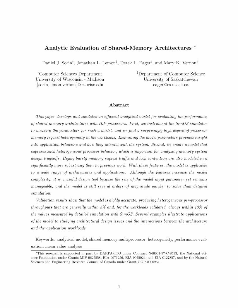
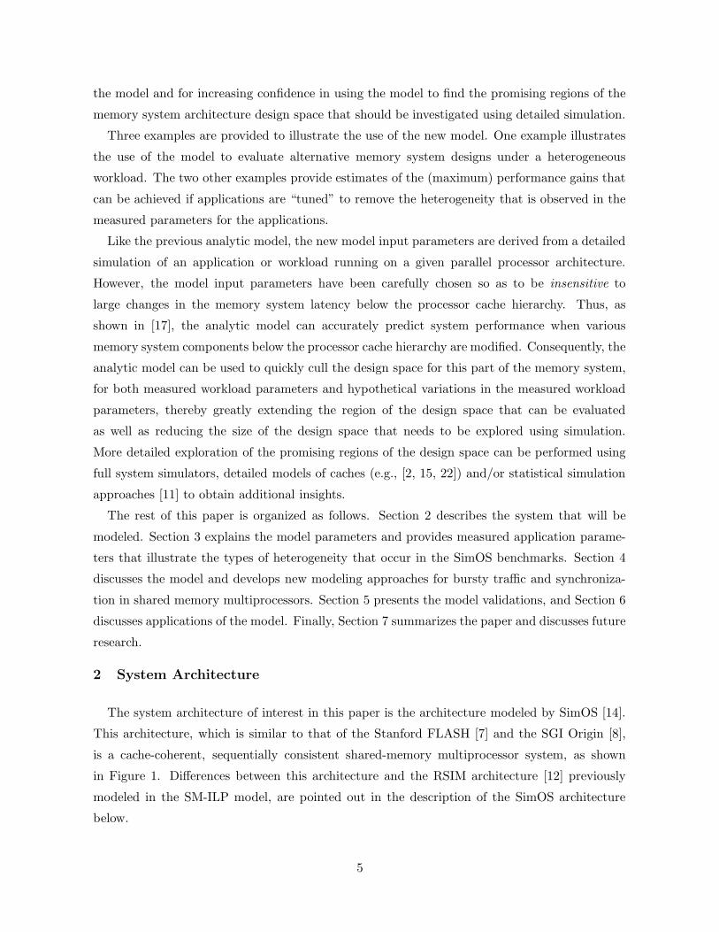
The system architecture of interest in this paper is the architecture modeled by SimOS [14].
This architecture, which is similar to that of the Stanford FLASH [7] and the SGI Origin [8],
is a cache-coherent, sequentially consistent shared-memory multiprocessor system, as shown
in Figure 1. Differences between this architecture and the RSIM architecture [12] previously
modeled in the SM-ILP model, are pointed out in the description of the SimOS architecture
below.
5
L1 Cache
L2 Cache
ProcessorILPComplex
Bus
DirectoryController
Mem
Figure 1. System Architecture
The MIPS R10000 processor, modeled by SimOS’s MXS simulator, is an aggressive implemen-
tation of sequential consistency (SC) that exploits instruction level parallelism using multiple
functional units, out-of-order execution, non-blocking loads, and speculative execution. Instruc-
tions are fetched into the instruction window, and they are issued to the functional units after
all of their input data dependences are satisfied. Speculative execution is used for (temporarily)
unresolved control dependences for up to four branch instructions. The instructions are fetched
into and retired from the window in program order, but they may be issued to the functional
units out of program order.
An instruction can retire from the instruction window only after it completes execution. A key
implication of this requirement is that when a load reaches the top of the instruction window,
retirement must stall if the data has not yet returned. SimOS differs from RSIM in that, since
SimOS models a sequentially consistent architecture, stores in SimOS only issue to the memory
system when they reach the top of the instruction window.
The caches use miss status holding registers (MSHRs) to track the status of all outstanding
misses [6]. Misses to the same cache line are coalesced in the MSHRs; only one memory request
is generated for such coalesced misses.
As shown in the figure, all traffic to or from a remote node goes through the directory controller
(DC). SimOS models the memory bus and the interconnection network using fixed latencies
that account for service time as well as estimated contention delay. In contrast to the RSIM
architecture, traffic into the node that only requires accessing the directory and memory does
not require use of the bus. SimOS also differs from RSIM in that it does not model a separate
network interface since the DC serves that purpose.
Cache coherence is maintained by a fairly standard three-state (MSI) directory-based invali-
6
parameter description value
N number of nodesm memory modules per node 1Mhw number of MSHRs 8Sbus bus latency 15SDC short directory controller (DC) latency 5SDClong
long directory controller latency 20
Snet average network traversal latency 30
Table 1. System Architecture Parameters
dation protocol. Unlike the RSIM architecture, cache-to-cache transfers require 4 hops instead
of 3; the home node is responsible for collecting invalidations before acknowledging a request for
exclusive permission.
3 Parameters
In this section, we describe the input parameters for the model. These parameters include
the system architecture parameters and the application parameters. Then we show that the ap-
plication parameters exhibit heterogeneity across the processors, and we explain several sources
of this heterogeneity.
3.1 System Architecture Parameters
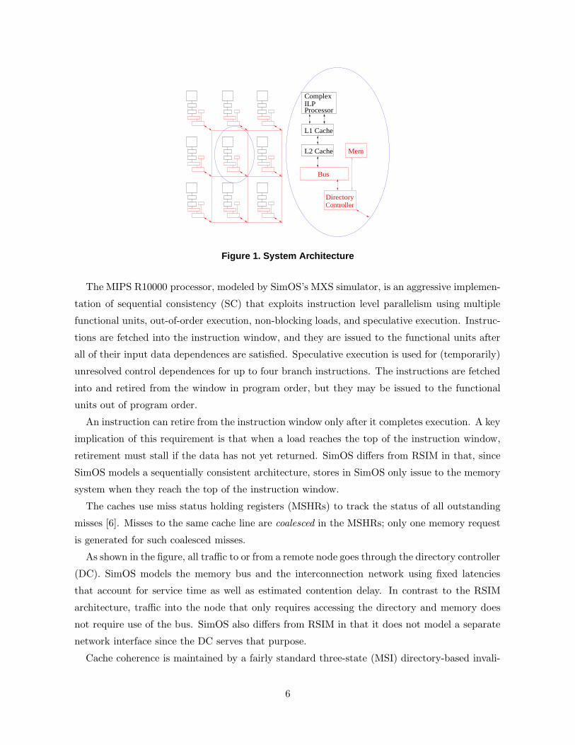
Table 1 defines the system architecture parameters, including the values that are used in the
validation experiments in Section 5. Latencies are in units of CPU cycles for the 200 MHz
R10000 processor. Note that memory access is overlapped with directory access; thus, there is
just one parameter for that access latency, SDClong.
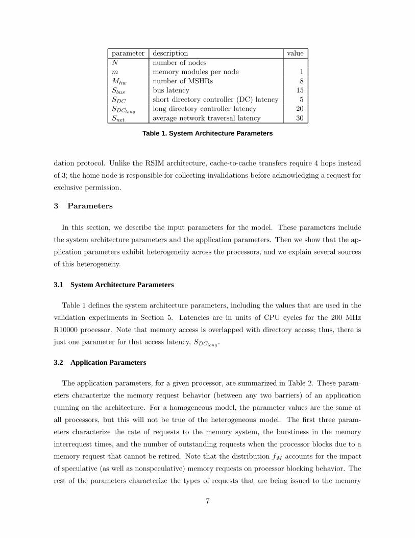
3.2 Application Parameters
The application parameters, for a given processor, are summarized in Table 2. These param-
eters characterize the memory request behavior (between any two barriers) of an application
running on the architecture. For a homogeneous model, the parameter values are the same at
all processors, but this will not be true of the heterogeneous model. The first three param-
eters characterize the rate of requests to the memory system, the burstiness in the memory
interrequest times, and the number of outstanding requests when the processor blocks due to a
memory request that cannot be retired. Note that the distribution fM accounts for the impact
of speculative (as well as nonspeculative) memory requests on processor blocking behavior. The
rest of the parameters characterize the types of requests that are being issued to the memory
7
Parameter Description
τ Average time between read, write, or upgrade requests to memory, not count-ing the time when the processor is completely stalled or is spin-waiting on asynchronization event
CVτ Coefficient of Variation of τfM Fraction of processor stalls that occur with M = 1, 2, ... outstanding requests
in the MSHRsPread, Pwrite, Pupgrade Probability that a memory request is a read, write, or upgradePwb Probability that a read or write request causes a writeback of a cache blockPL|x Probability directory is local for a type x transaction; x=read, write, upgrade,
writebackPM |x,y Probability home memory can supply the data for a type x, y request;
x=read, write; y=local home, remote homeP4hop|x¬−memory Probability that a request of type x to a remote home is forwarded to a cache
at a third node;x=read,write
X Average number of invalidates caused by a write or upgrade to a clean line
Table 2. Application Parameters
system. Sorin et al. observe that these input parameters are sensitive to instruction window
size, processor architecture, organization and size of the processor cache hierarchy, and various
aspects of the application code and compiler, but are relatively insensitive to memory system
latencies below the processor cache hierarchy [17].
3.3 Heterogeneity in Application Parameters
The homogeneous SM-ILP model assumes that all processors have statistically similar ap-
plication behavior with respect to the memory system and that each processor’s local/remote
memory accesses are uniformly distributed across the local/remote memory modules. In the
homogeneous model, each processor has the same input parameters, as shown in Table 2, and
no input parameters are needed for frequencies of access to each memory module.
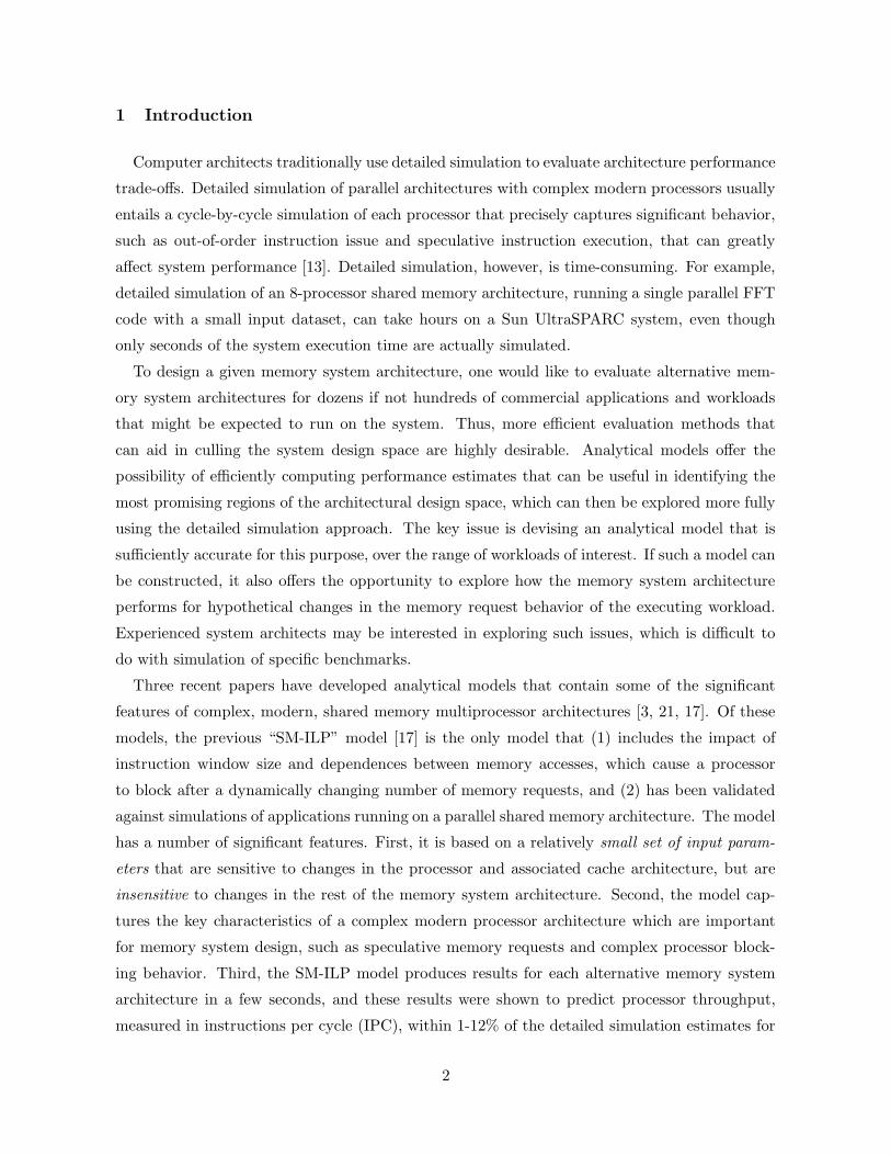
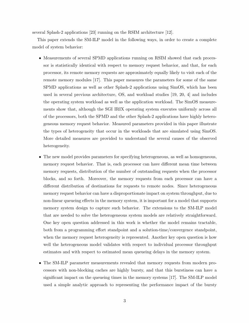
Figures 2, 3, and 4 illustrate the processor heterogeneity in several key parameters for par-
ticular barriers (i.e., inter-barrier phases) of a few SPLASH-2 benchmarks [23], as measured by
SimOS. The benchmark name is followed by the number of processors, e.g, FFT-8 is an eight
processor run of the FFT benchmark. For each input parameter shown, the eight bars repre-
sent the values of that parameter for each of the eight processors, divided by the value of that
parameter when measured over all eight processors. The heterogeneity in various measures for
particular barriers is also summarized in Table 3.
The degree of parameter heterogeneity, such as in the measures of τ and P (L|w) in the figures
and Table 3, is perhaps higher than might be expected. Some (irregular) applications, such as
Radiosity, are inherently heterogeneous, and thus the per-processor memory request measures
8
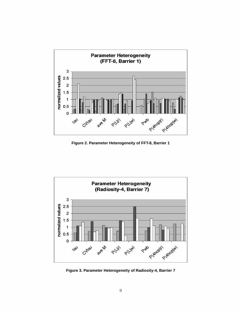
Figure 2. Parameter Heterogeneity of FFT-8, Barrier 1
Figure 3. Parameter Heterogeneity of Radiosity-4, Barrier 7
9
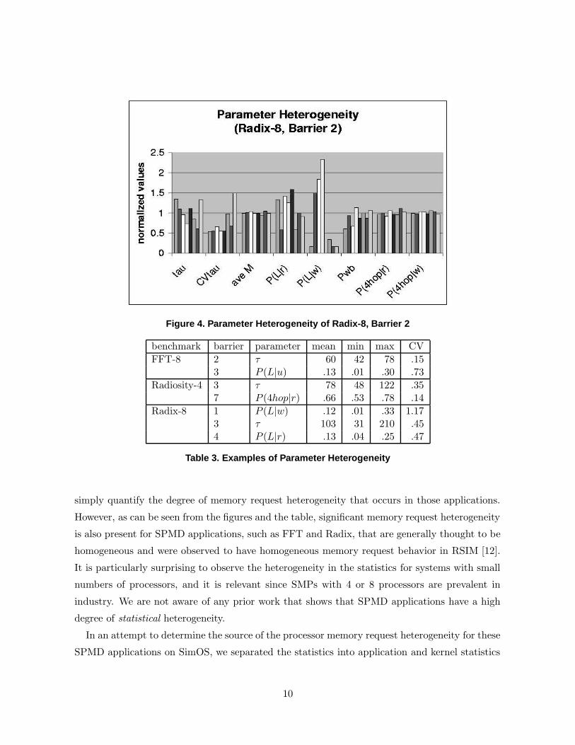
Figure 4. Parameter Heterogeneity of Radix-8, Barrier 2
benchmark barrier parameter mean min max CV
FFT-8 2 τ 60 42 78 .153 P (L|u) .13 .01 .30 .73
Radiosity-4 3 τ 78 48 122 .357 P (4hop|r) .66 .53 .78 .14
Radix-8 1 P (L|w) .12 .01 .33 1.173 τ 103 31 210 .454 P (L|r) .13 .04 .25 .47
Table 3. Examples of Parameter Heterogeneity
simply quantify the degree of memory request heterogeneity that occurs in those applications.
However, as can be seen from the figures and the table, significant memory request heterogeneity
is also present for SPMD applications, such as FFT and Radix, that are generally thought to be
homogeneous and were observed to have homogeneous memory request behavior in RSIM [12].
It is particularly surprising to observe the heterogeneity in the statistics for systems with small
numbers of processors, and it is relevant since SMPs with 4 or 8 processors are prevalent in
industry. We are not aware of any prior work that shows that SPMD applications have a high
degree of statistical heterogeneity.
In an attempt to determine the source of the processor memory request heterogeneity for these
SPMD applications on SimOS, we separated the statistics into application and kernel statistics
10
for each processor. For example, the number of memory requests per processor for the transpose
phase (barrier 2) of FFT-4 is shown in Table 4. As expected, the number of memory requests
that are issued when a processor is executing the application are quite homogeneous across the
processors, with a coefficient of variation of 0.02. What is perhaps surprising is both the high
numbers of memory requests that are issued in kernel mode (larger, in fact, than the numbers
of application requests) as well as the heterogeneity in this number across processors, as shown
by a coefficient of variation of 0.27. For the SPMD applications, other parameters like CVτ ,
exhibit similar heterogeneity in the kernel while remaining homogeneous in the application.1
A key point is that the kernel executes uniformly across the processors in the SimOS architec-
ture, and thus the kernel memory request statistics are fairly homogeneous across the processors
if measured over a long time interval, such as the execution time for the entire application. How-
ever, the memory request heterogeneity observed in the measured intervals between each barrier
will impact memory system performance, and, therefore, the heterogeneity in this timeframe
must be measured and represented in the inputs to the model.
cpu 0 cpu 1 cpu 2 cpu 3
overall 461 613 781 787
application 216 219 231 219kernel 245 394 550 568
Table 4. Memory Requests for FFT-4 Barrier 2
Beyond the heterogeneity inherent in some applications or caused by kernel behavior, some
applications can exhibit heterogeneous behavior if they have not been “tuned” to run on a
particular architecture and runtime system, which occurs frequently in practice. Heterogeneity
in the measured model input parameters can point to the need for such tuning, and even indicate
what types of tuning are needed. For example, in barrier 1 of FFT-8, three processors have small
relative values of τ when the application is executing, indicating that they have especially high
level 2 cache miss rates. Those same processors (and one additional processor) have a relatively
low probability of local memory access for read and/or write requests. Thus, examining the data
layout or comparing the code that runs on those three processors against the code that runs
on the other five processors, looking for differences that might cause these effects, may lead to
some insight about how to improve performance. Similarly, the heterogeneity in the probability
that a write request is local for Radix suggests that data layout should be examined for that
application as well.
1Note that in Table 4, the number of memory requests appears to be correlated with the processor number,but this correlation is just coincidental and did not occur with any higher than random frequency in the resultsthat we obtained for different barriers in the FFT application and for different applications.
11
In general, although there may be intuition that particular applications will exhibit heteroge-
neous behavior of some form, intuition alone is generally insufficient to estimate the magnitude
of the heterogeneity in particular statistics of interest, its magnitude relative to the heterogeneity
induced by kernel activity, or the extent to which performance might be improved by particular
types of application tuning. Measurements of heterogeneity, and the use of models that capture
its performance impacts, can provide answers to such questions.
The figures and the table indicate that heterogeneity occurs in practice for every model input
parameter. Two parameters, though, have notably less extreme heterogeneity: (1) the average
of the fM distribution (i.e., the average number of memory requests that are outstanding when
the processor blocks because a load or store cannot be retired) and (2) the probability that a
remote read request for a dirty block requires invalidating or downgrading the line in a cache
at another remote node (P4hop|r). However, system performance can be sensitive to the values
of these parameters. Thus, the model extensions for processor heterogeneity will allow each
processor to have its own value for each of the input parameters.
3.4 Methodology for Obtaining the Application Parameters
As mentioned in Section 3.2, previous work has shown that the homogeneous model input pa-
rameters are, to first order, insensitive to changes in memory system latency below the processor
cache hierarchy. For the new model developed in this paper, we use the same input parameters
for each processor, but allow each processor to have a different value for each parameter. Thus,
these input parameters will also be insensitive (to first order) to changes in the memory system
latencies below the processor-cache hierarchy. One question is whether these parameters are
sufficient for accurately computing processor throughputs and mean delays in the memory sys-
tem for heterogeneous workloads. This question will be investigated by comparing the estimates
against the performance measures that are given by SimOS.
The set of parameters for a given application/workload of interest executing on a given pro-
cessor and cache architecture of interest are obtained through simulation of the application on a
single memory and interconnection network architecture (e.g., an idealized constant latency in-
terconnect) with memory access latencies that are within a small constant factor of the latencies
in the memory architectures to be evaluated with the model. Currently, as shown in [17], the
most accurate way to estimate these parameters is to use the detailed simulator (e.g., SimOS)
that will be used to further evaluate the promising memory system architectures identified by
the analytic model. 2
2Faster methods might be developed to obtain some of the parameters, as was investigated for the SM-ILPmodel, but those parameters have so far been less accurate than the parameters from the detailed simulator, andimprovements in the faster simulation methods are beyond the scope of this paper.
12
A key point in this methodology is that the detailed simulator is run once for each workload
and a given processor/cache architecture to obtain the analytic model parameters. The analytic
model is then used to evaluate many candidate memory and interconnection network architec-
tures, as illustrated in Section 6 of the paper. The detailed simulator is then used to evaluate
further details of the most promising memory/interconnect architectures. Because the detailed
simulator is needed for detailed analysis of the more promising architectures, the one run needed
per application to obtain the parameters for the analytic model does not add significantly to
the total time needed to evaluate the architectures. Conversely, the analytic model is more
easily modified for alternative memory/interconnect architectures than the simulator (because
the analytic model is more abstract and the equations each have one of several possible forms),
and it can significantly speed up evaluation of the alternative architectures.
4 Analytical Model
In this section, we develope the extended analytical model for the SimOS architecture. The
principal output measure computed by the model is the system throughput, measured in instruc-
tions retired per cycle (IPC). This throughput, as well as mean waiting time and utilization of
each memory system resource, is computed as a function of the input parameters that charac-
terize the workload and the memory architecture.
For simplicity in the exposition of the model equations, we first present the homogeneous
model in Section 4.1, and then present the extensions for the heterogeneous model in Section 4.2.
In Section 4.3, we develop the techniques for modeling bursty memory traffic and lock contention.
4.1 Homogeneous Model
As in the previous SM-ILP model [17] we develop a customized Approximate Mean Value
Analysis (AMVA) model of homogeneous workloads running on the SimOS architecture. Our
experience is that, as claimed in that paper, it is not difficult to modify the basic AMVA
equations in the previous model [18] for other shared memory multiprocessor architectures. The
most significant issue in developing the new model was how to model the different memory
consistency model in the SimOS architecture. Unlike the SM-ILP model which iterated between
two submodels to account for two types of processor blocking behavior in the release consistent
(RC) RSIM architecture, the model of the sequentially consistent (SC) SimOS architecture
developed below is a single model that accounts for all types of blocking behavior.
The processor and cache subsystem are modeled as a black box that - when not completely
stalled - issues memory requests at a given rate (1/τ) and with a given coefficient of variation
in interrequest times (CVτ ). The model computes the overall mean system residence time for
13
a memory request, including mean delays and service times at the directory controllers (DCs),
split-transaction memory buses, and in the interconnection network.
For readability, we have adopted the following notation of subscripts and superscripts for the
variables in the model. The resource is always the first subscript on a variable, whether it is
mean residence time (R), mean waiting time (W ), mean utilization (U), or mean service time
(S). For example, Rdc is the mean residence time at the directory controller. For many terms,
there is a subscript of loc or rem to indicate whether the resource is at the local node for a
given processor or a remote node. The subscript variable y denotes the transaction type (such
as read or write). We first present the equations for the case that fM = 1 for a particular but
arbitrary value of M less than or equal to the number of MSHRs. In this case each processor has
M customers that each alternately visit the processor for average time τ and then visit various
resources in the memory system, reflecting (statistically) the memory request behavior from the
processor. Later we discuss how to model the more general distribution for fM .
The following equation is for the total mean residence time of a customer for one cycle
from the processor, through the memory system, and back to the processor. This includes the
mean residence times at the processor, buses (both local and remote), network, and directory
controllers.
R = Rpe + Rbus + Rnet + Rdc
Each of these terms is derived from lower level equations. For example, the mean residence
time at the directory controllers is equal to the sum of the mean residence time at the local DC
and at the remote DCs.
Rdc = Rdcloc+ Rdcrem
The mean residence time at the local (remote) DC is equal to the sum of the weighted mean
residence time for each transaction type y at the local (remote) DC, weighted by the probability
that the transaction is of type y.
Rdcloc=∑
y
Rdcloc,y
Rdcrem=∑
y
Rdcrem,y
The weighted mean residence time of a transaction of type y at the local (remote) DC is equal
to the probability of transaction y times the average number of visits the type y transaction
makes to the local (remote) DC (Vdirlocy) times the sum of the waiting time at the local (remote)
DC (Wdcloc) and the service time at a DC.
14
Rdcloc,y= PyVdclocy
(Wdcloc+ Sdc)
Rdcrem,y= PyVdcremy
(Wdcrem+ Sdc)
Note that the average number of visits to the local (remote) DC is computed for the transac-
tion type using the other probabilities given in Table 2.
All of the terms in the above equations are inputs except the waiting times. Wdclocconsists
of the waiting time at the local DC due to requests from the local node (W locdcloc
) and due to
requests from remote nodes (W remdcloc
).
Wdcloc= W loc
dcloc+ W rem
dcloc
The waiting time at the local DC due to requests from the local node equals the sum of the
waiting times over all transaction types y that cause waiting.
W locdcloc
=∑
y
W loc,ydcloc
W remdcloc
=∑
y
W rem,ydcloc
Wdcremconsists of the waiting time due to remote customers that are not from that remote
node (W othersdcrem
) and those that are from that remote node (W remdirrem
).
Wdcrem= W others
dcrem+ W rem
dcrem
W othersdcrem
=∑
y
W others,ydcrem
W remdcrem
=∑
y
W rem,ydcrem
The following equations are for the mean waiting times due to waiting for specific transaction
types. For example, W loc,ydcloc
is the mean waiting time at the local DC due to local requests
of transaction type y. Mean waiting time for a single other customer equalsRdcloc,y
R− Udcloc,y
(the probability that a customer is in the queue but not in service) times the service time, plus
Udcloc,y(the probability that a customer is in service) times the mean residual life of a customer
15
in service. Therefore, to get the total mean waiting time, we multiply by the number of local
customers who could cause an arriving local customer to wait, M − 1.
W loc,ydcloc
= (M − 1)
[(
Rdcloc,y
R− Udcloc,y
)
Sdc + Udcloc,y
(
Sdc
2
)]
W rem,ydcloc
= M(N − 1)
[(
Rdcrem,y
R− Udcrem,y
)
Sdc + Udcrem,y
(
Sdc
2
)]
W others,ydcrem
= [(M − 1) + M(N − 2)][(Rdcrem,y
R− Udcrem,y
)Sdc + (Udcrem,y)(
Sdc
2)]
W rem,ydcrem
= M [(Rdcloc,y
R− Udcloc,y
)Sdc + (Udcloc,y)(
Sdc
2)]
Lastly, we have the utilization equations. The first equation is the mean utilization of a DC by
a local customer, and the second equation is the mean utilization of a DC by a remote customer.
Udcloc,y=
Py
R(Vdcloc,y
Sdc)
Udcrem,y=
Py
R(Vdcrem,y
Sdc)
A key question in developing the analytic model is how to compute throughput as a function
of the dynamically changing number of outstanding memory requests that can be issued before
the processor must stall waiting for data to return from memory. The SM-ILP model resolved
this issue by solving the model for each value of M and then taking a weighted average of the
results. As will be explained in the next section, a different solution will be necessary for a
heterogeneous model.
4.2 Modeling Heterogeneity
Given that (1) processor heterogeneity (and memory access non-uniformity) occur quite fre-
quently in practice, and (2) the heterogeneity can be expected to have a non-linear impact on
queueing and memory system performance, this section extends the model above for hetero-
geneous workloads. Results in Section 5 will show that modeling heterogeneity is critical for
achieving accurate results.
Three features are needed in order to model heterogeneous processor behavior. First, new
model inputs are required. Specifically, each of the model input parameters in Table 2 is mea-
sured for each processor. Also, modeling memory access non-uniformity requires additional
16
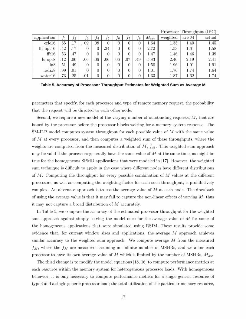
Processor Throughput (IPC)
application f1 f2 f3 f4 f5 f6 f7 f8 Mave weighted ave M actual
erle16 .65 .17 . 09 .08 0 0 0 0 1.64 1.35 1.40 1.45fft-opt16 .42 .17 0 0 .34 0 0 0 2.72 1.53 1.61 1.58
fft16 .53 .47 0 0 0 0 0 0 1.47 1.46 1.46 1.39lu-opt8 .12 .06 .06 .06 .06 .06 .07 .49 5.83 2.46 2.19 2.41
lu8 .51 .49 0 0 0 0 0 0 1.50 1.96 1.91 1.91radix8 .99 .01 0 0 0 0 0 0 1.01 1.76 1.74 1.64
water16 .73 .25 .01 0 0 0 0 0 1.33 1.87 1.62 1.74
Table 5. Accuracy of Processor Throughput Estimates for Weighted Sum vs Average M
parameters that specify, for each processor and type of remote memory request, the probability
that the request will be directed to each other node.
Second, we require a new model of the varying number of outstanding requests, M , that are
issued by the processor before the processor blocks waiting for a memory system response. The
SM-ILP model computes system throughput for each possible value of M with the same value
of M at every processor, and then computes a weighted sum of these throughputs, where the
weights are computed from the measured distribution of M , fM . This weighted sum approach
may be valid if the processors generally have the same value of M at the same time, as might be
true for the homogeneous SPMD applications that were modeled in [17]. However, the weighted
sum technique is difficult to apply in the case where different nodes have different distributions
of M . Computing the throughput for every possible combination of M values at the different
processors, as well as computing the weighting factor for each such throughput, is prohibitively
complex. An alternate approach is to use the average value of M at each node. The drawback
of using the average value is that it may fail to capture the non-linear effects of varying M ; thus
it may not capture a broad distribution of M accurately.
In Table 5, we compare the accuracy of the estimated processor throughput for the weighted
sum approach against simply solving the model once for the average value of M for some of
the homogeneous applications that were simulated using RSIM. These results provide some
evidence that, for current window sizes and applications, the average M approach achieves
similar accuracy to the weighted sum approach. We compute average M from the measured
fM , where the fM are measured assuming an infinite number of MSHRs, and we allow each
processor to have its own average value of M which is limited by the number of MSHRs, Mhw.
The third change is to modify the model equations [18, 16] to compute performance metrics at
each resource within the memory system for heterogeneous processor loads. With homogeneous
behavior, it is only necessary to compute performance metrics for a single generic resource of
type i and a single generic processor load; the total utilization of the particular memory resource,
17
for example, can then be obtained simply by multiplying by the number of processors. This
leads to model complexity on the order of the number of types of resources, as was seen in
the equations in Section 4.1. For heterogeneous processor loads, in contrast, each processor
may have differing memory referencing behavior and thus may contribute to differing extents to
utilization and contention at each resource. Computing the N 2 interactions of each processor
on each memory system resource increases the complexity of the model equations by a factor of
N2, which leads to a key question about whether the iterative model will converge in practice.
This issue is addressed in Section 5. Efficient coding methods (for both the homogeneous and
heterogeneous model) limit the size of the model (measured in C++ code), though, to only
about twice that of the homogeneous model. The accuracy improvements that may be obtained
by accurately modeling heterogeneous memory request behavior when it exists, rather than
assuming homogeneity, are also illustrated in Section 5.
At a high level, the heterogeneous equations have form similar to the homogeneous equations.
Terms require extra indices (given in brackets) to indicate the node of the customer and/or
the destination. Thus, a utilization term such as Udcloc(the mean utilization of the local DC)
becomes Udcloc[i] (the mean utilization of the DC of node i by local customers) to reflect the
fact that the utilization of the local DC is different for different nodes. The probabilities of the
transaction types (e.g., local read or 4-hop write) use an index in a similar fashion. For example,
we now have that the probability of transaction y at node i is Py[i]. So, the total mean residence
time for a customer from node i, R[i], is equal to the sum of its mean residence times at the
processor (pe), buses, network, and directory controllers (dc).
R[i] = Rpe[i] + Rbus[i] + Rnet[i] + Rdc[i]
Examining the DC portion of this equation highlights the differences in the equations between
the heterogeneous and homogeneous models. Mean DC residence time is equal to the mean
residence time at the local DC plus the mean residence time at the DCs of the other nodes.
Rdc[i] = Rdcloc[i] +
∑
j
j 6=i
Rdcrem[i][j]
Only focusing on the mean residence time at the remote DC, it is the sum of the mean
residence times over the different types of transactions, denoted by a subscript of y.
Rdcrem[i][j] =
∑
y
Rdcrem,y[i][j]
The mean residence times of individual transaction types are equal to the probability of the
transaction type (Py[i]) times the visit count (Vdcremy[i][j]) times the sum of the mean waiting
time (Wdcrem[i][j]) and the service time at the DC (Sdc):
18
Rdcrem,y[i][j] = Py[i]Vdcremy
[i][j](Wdcrem[i][j] + Sdc)
All of the terms in the above equation are inputs except for the waiting times. The equation
for mean waiting time at a remote directory is as follows:
Wdcrem[i][j] = W others
dcrem[i][j] + W rem
dcrem[i][j]
W othersdcrem
[i][j] is the mean waiting time of a node i customer at the DC of node j due to traffic
from all nodes other than node j. W remdcrem
[i][j] is the mean waiting time of a node i customer at
the DC of node j due to traffic from node j. Only breaking down W remdcrem
[i][j] further, we have
that
W remdcrem
[i][j] =∑
y
(
W rem,ydcrem
[i][j])
The following equations are for the mean waiting times of specific transaction types. Thus,
W rem,ydcrem
[i][j] is the mean waiting time by a node i customer at node j’s DC due to node j
traffic for transactions of type y. Mean waiting time due to a single node j customer equalsRdcloc,y
[j]
R[j] − Udcloc,y[j] (the probability that a customer is in the queue but not in service) times
the service time, plus Udcloc,y[j] (the probability that a customer is in service) times the mean
residual life of a customer in service. Therefore, to get the total mean waiting time, we multiply
by the number of node j customers, M [j].
W rem,ydcrem
[i][j] = M [j]
[(
Rdcloc,y[j]
R[j]− Udcloc,y
[j]
)
Sdc + Udcloc,y[j]
(
Sdc
2
)
]
Lastly, we have the equation for the mean utilization of node i’s DC by a local customer.
Udcloc,y[i] =
Py[i]
R[i](Vdcloc,y
[i]Sdc)
Modeling the other resources in the system is similar to what has been shown here for the
DC. All of the details of the heterogeneous AMVA equations can be found in [16].
4.3 Modeling Bursty Memory Requests and Lock Contention
In this section, we present two further model extensions. In Section 4.3.1, we adapt the new
AMVA techniques proposed in [5] to model bursty memory request traffic observed in the SimOS
workload measures. In Section 4.3.2, we develop a method for computing lock synchronization
from basic model input parameters.
19
4.3.1 Burstiness
In the previous SM-ILP model, the mean residual linfe of a “customer in service” at the processor
(i.e., a memory request about to be generated) is computed using an intuitively motivated ad hoc
interpolation. In this paper, we instead employ a new and significantly more accurate AMVA
technique (called “AMVA-decomp”) [5] for computing mean residence time at the processor
queue. In addition, we adapt the new AMVA techniques in [5] for computing the mean wait at
the “downstream” queue (i.e., the local DC in the SimOS architecture) which has bursty arrivals
from the local processor, and thus increased average queueing delay compared with the random
arrivals assumed in the standard AMVA equations.
The use of these new simple AMVA techniques is motivated by the fact that they represent
a very favorable balance between accuracy, efficiency, and robustness. Most importantly, they
are based on a small number of input parameters for which reliable values are relatively easy to
obtain. Furthermore, the solution method is easy to implement and does not add appreciable
complexity to the overall AMVA model solution. Finally, the technique is shown in [5] to have
very high accuracy over a wide range of system parameters, including parameter values for
which it might be expected to have high inaccuracy. More detailed models of the processor
service times, with correspondingly more detailed models of the DC arrival process, could be
constructed, but such models would require more detailed input parameters that would be
more difficult to estimate reliably. The more detailed model would also be more complex to
implement, and thus would only be justified if an appreciable increase in model accuracy could
be expected. However, mean delays and system throughput for closed systems are not sensitive
to the details of the service distributions (i.e., higher moments of the distribution than the
first or second moment) at the various resources in the system [9, 10]. Thus, a more detailed
model of the processor service time distribution is not desirable. Validation results later in the
paper confirm that, for the purposes of computing system throughput for alternative memory
system architectures, the simple AMVA techniques outlined below, capture the bursty behavior
in sufficient detail to predict system throughput quite accurately.
The AMVA-decomp technique assumes that the server that has the bursty departures (i.e.,
the processor nodes in the SimOS architecture) can be modeled with a 2-stage hyperexponential
distribution of service times. That is, with probability p a given customer has a “small” mean
service time, τa, and with probability 1 − p the customer has a “large” mean service time,
τb, where τa < τb and τ = pτa + (1 − p)τb. The key question in applying this technique
for the processors in the heterogeneous model is how to obtain the parameters of a suitable
hyperexponential distribution. Two constraints on the distribution are the measured mean
service time (τ) and the coefficient of variation in the service time (CVτ ). However, this is an
20
underconstrained problem. To apply this technique to modeling heterogeneous bursty processors,
we define a third parameter for each processor, τa, that is equal to the minimum measured value
of τ .3 Using τ , CVτ , and τa, we solve for τb and p.
In the model of bursty requests at the downstream queues, there are bursts of arrivals and
intervals between bursts in which there are no arrivals. This scenario is characterized by three
parameters:
k, the average number of customer arrivals within a burst,
Ii, the mean interarrival time within a burst, and
Io, the mean time between bursts.
In applying the bursty request model to the local DCs in the SimOS architecture, the key
question again is how to map the requisite parameters to observable quantities in the system.
There are two constraints in determining values for these three parameters. First, the coefficient
of variation in the interarrival time is determined by the coefficient of variation in the service
time at the processor. Second, the throughput at the downstream queue, and thus the mean
interarrival time, is determined during the AMVA solution. We create a third constraint by
setting Ii equal to the value of τa, since it is reasonable to assume that interarrival time during a
burst would be similar to the value of a short service time at the processor. We also assume that
downstream burstiness is only caused by requests from the local processor. The superposition
of requests from other processors will, on average, be less bursty.
Solving the model with the burstiness equations initially led to some convergence problems.
Ensuring that the model converges requires some careful choices of initial values and bounds
on the input parameters to make sure that values produced during the iterative solutions are
reasonable. For example, k cannot be allowed to be larger than the total number of local
customers.
4.3.2 Lock Contention
The previous SM-ILP model measured average lock waiting times, which are affected by the
memory system architecture, instead of computing these performance measures from more ba-
sic parameters that are independent of the memory system architecture. In this paper, lock
synchronization effects are computed from basic inputs with a separate lock contention model.
Contention for a particular lock is most naturally modeled by a queue in which the server is
the lock and the service time is the lock holding time. The challenge in constucting this queue
3Note that other choices to τa, such as a small constant times the minimum measured value of τ , are alsopossible. What’s needed is a value that is approximately correct. We choose to set τa to a measured value andallow τb to be computed from τa because the best value of the “small” mean is likely to be near the measuredminimum value of τ , while there is no measured value that corresponds well to τb. Moreover, the model is moresensitive to the value of τa than to that of τb, especially in the high variance cases where τa << τb.
21
for the memory system architecture workloads is that the customers (i.e., application processes)
queue for the lock while in service at the processor. Furthermore, while holding the lock, the
customer may queue for memory system resources and then for further use of the processor. In
addition, the program can release the lock while still holding the processor and it can complete
service at a memory system resource or processor while still holding the lock. To model these
various behaviors, we initially assume that only one lock is held at a time, and then relax this
assumption.
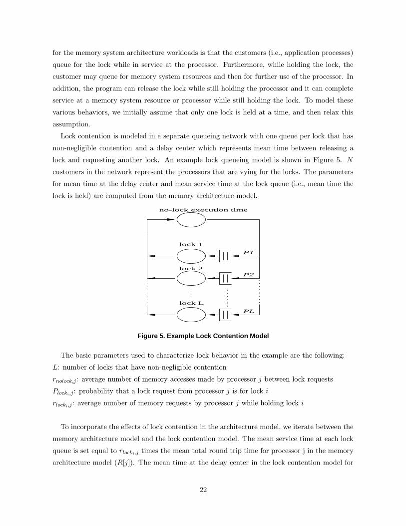
Lock contention is modeled in a separate queueing network with one queue per lock that has
non-negligible contention and a delay center which represents mean time between releasing a
lock and requesting another lock. An example lock queueing model is shown in Figure 5. N
customers in the network represent the processors that are vying for the locks. The parameters
for mean time at the delay center and mean service time at the lock queue (i.e., mean time the
lock is held) are computed from the memory architecture model.
lock 1
lock 2
lock L
P1
P2
PL
no-lock execution time
Figure 5. Example Lock Contention Model
The basic parameters used to characterize lock behavior in the example are the following:
L: number of locks that have non-negligible contention
rnolock,j: average number of memory accesses made by processor j between lock requests
Plocki,j: probability that a lock request from processor j is for lock i
rlocki,j: average number of memory requests by processor j while holding lock i
To incorporate the effects of lock contention in the architecture model, we iterate between the
memory architecture model and the lock contention model. The mean service time at each lock
queue is set equal to rlocki,j times the mean total round trip time for processor j in the memory
architecture model (R[j]). The mean time at the delay center in the lock contention model for
22
customer j is set equal to rnolock,j times R[j]. The mean service time at the processor in the
architecture model is inflated (i.e., increased to τj + τj/rnolock,j), to include mean lock waiting
time computed from the lock model. The iterative solution again increases the complexity of
the model, an issue that will be addressed in Section 5. It also causes solution time to increase
slightly, but solution time is still on the order of seconds. Moreover, this iterative technique
can be generalized for specific cases of nested lock requests by having a separate lock contention
model for the locks at each level of the lock hierarchy and iteratively solving the lock models
along with the architecture model. The details of the lock contention equations can be found
in [16].
5 Model Validation
In this section, we present the results of validation experiments that assess the accuracy of the
analytic model that is developed in this paper. The validations are performed against SimOS,
using SimOS’ detailed MXS processor simulator and its NUMA memory system simulator.
SimOS runs IRIX 5.3, and all benchmark results include OS behavior that occurred while
the benchmark was running. Thus, we measure analytic model inputs and estimate system
performance for the complete system behavior, instead of for the application alone.
The validation experiments include FFT, LU, Radiosity, and Radix from the Splash-2 suite [23].
Table 6 shows the data sets used for each application. We attempted to obtain SimOS results for
the rest of the Splash-2 benchmark suite, but these applications would not run successfully on
the version of the SimOS MXS processor simulator used in this study. (This version of the MXS
simulator was one of the first versions to be released for use outside of the research group that
developed and initially used the simulator for architectural studies. Thus, various steps needed
to get the other applications to run may have been missing from the available documentation.)
Similarly, we were unable to make this version of the SimOS MXS simulator produce results for
greater than 8 processors. Although the number of benchmarks that ran successfully is small, the
memory access characteristics captured in the model input parameters vary greatly across these
applications as well as in the different periods between barriers in a given application, and thus
the analytical model is exercised over a non-trivial region of the input parameter space. Tables 3
and 5 illustrate some of the variety in the memory request behavior across the applications. As
we will show later, the processor throughput varies from 0.1 to 2.4 instructions per cycle across
the application barriers against which we were able to validate, indicating that the differences in
memory request behavior among these benchmarks is significant. The low processor throughput
estimates also indicate that, although the number of processors is relatively small, significant
contention occurs in the memory system (particularly at the directory controllers), and thus
23
app input size
FFT -l6 -n1024LU 512x512 array, 16x16 blocksRadiosity -batchRadix 1M integers, radix 1024
Table 6. Benchmark Data Sets
the ability of the analytic model to accurately estimate queueing delays is also exercised. This
is confirmed by the measured mean queueing delays reported by SimOS for these applications
(with the architectural parameters in Table 1).
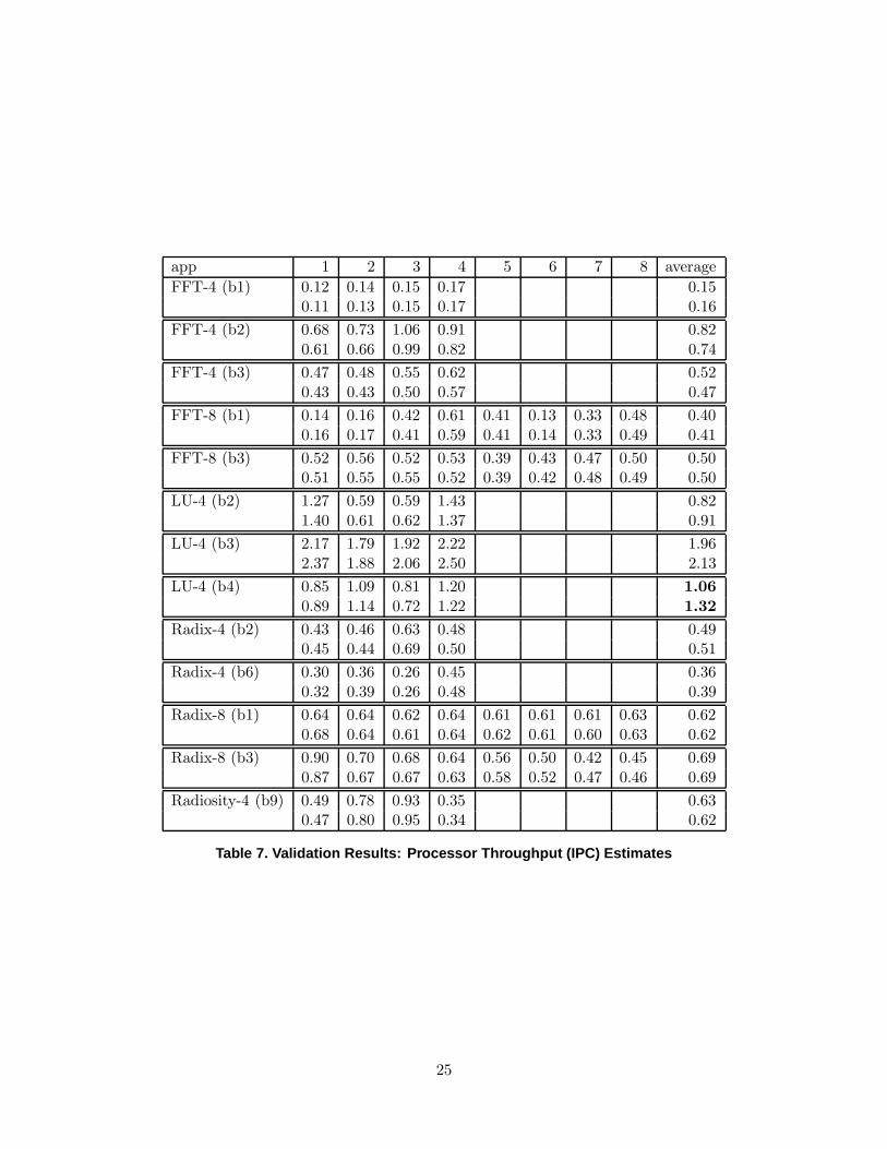
The validation results for model input parameter values that exhibited the greatest degrees
of heterogeneity in processor performance are shown in Figures 6, 7, and 8. These results are
for specific barriers (i.e., inter-barrier phases) of FFT, Radix, and Radiosity, running on 8-node
and 4-node versions of SimOS. Each graph gives the throughput (in IPC) for each processor
estimated by the new heterogeneous system model as well as the average throughput estimated
by the homogeneous model. Results for other barriers of the FFT, LU, Radix, and Radiosity
benchmarks (both 8-node and 4-node) are presented in Table 7. The column numbers in the
table correspond to node numbers. For each pair of rows, the first row is the IPC reported
by SimOS, and the second row is the IPC predicted by the model. The rightmost column
corresponds to a homogeneous model using the average statistics, where the first row is the
average IPC across all nodes reported by SimOS, and the second row is the IPC predicted by
the previous homogeneous model using input parameters that are averaged across all nodes.
These results show that the analytic estimates of per-processor throughput agree quite closely
with the SimOS measurements, even when each processor throughput is remarkably different.
The model achieves accurate performance estimates although memory request behavior is mod-
eled statistically and at a high level of abstraction. As mentioned before, the complexity of the
new analytic model makes its tractability a key question. In validating the model, however, we
discovered no cases where the model did not converge to a solution within a matter of a few
seconds, in spite of strong heterogeneity in the model inputs and in the estimated per-processor
throughputs.
Although the homogeneous analytic model is also often accurate in estimating the average
processor throughput, the new estimates of per-processor throughput from the heterogeneous
model are crucial to accurately estimating the impact of the memory system architecture on
application execution times, because for applications employing barriers, the barrier only com-
pletes execution when the slowest processor reaches the barrier. Moreover, there are examples,
such as LU-4 barrier 4, for which the homogeneous model is not even accurate with respect to
24
app 1 2 3 4 5 6 7 8 average
FFT-4 (b1) 0.12 0.14 0.15 0.17 0.150.11 0.13 0.15 0.17 0.16
FFT-4 (b2) 0.68 0.73 1.06 0.91 0.820.61 0.66 0.99 0.82 0.74
FFT-4 (b3) 0.47 0.48 0.55 0.62 0.520.43 0.43 0.50 0.57 0.47
FFT-8 (b1) 0.14 0.16 0.42 0.61 0.41 0.13 0.33 0.48 0.400.16 0.17 0.41 0.59 0.41 0.14 0.33 0.49 0.41
FFT-8 (b3) 0.52 0.56 0.52 0.53 0.39 0.43 0.47 0.50 0.500.51 0.55 0.55 0.52 0.39 0.42 0.48 0.49 0.50
LU-4 (b2) 1.27 0.59 0.59 1.43 0.821.40 0.61 0.62 1.37 0.91
LU-4 (b3) 2.17 1.79 1.92 2.22 1.962.37 1.88 2.06 2.50 2.13
LU-4 (b4) 0.85 1.09 0.81 1.20 1.06
0.89 1.14 0.72 1.22 1.32
Radix-4 (b2) 0.43 0.46 0.63 0.48 0.490.45 0.44 0.69 0.50 0.51
Radix-4 (b6) 0.30 0.36 0.26 0.45 0.360.32 0.39 0.26 0.48 0.39
Radix-8 (b1) 0.64 0.64 0.62 0.64 0.61 0.61 0.61 0.63 0.620.68 0.64 0.61 0.64 0.62 0.61 0.60 0.63 0.62
Radix-8 (b3) 0.90 0.70 0.68 0.64 0.56 0.50 0.42 0.45 0.690.87 0.67 0.67 0.63 0.58 0.52 0.47 0.46 0.69
Radiosity-4 (b9) 0.49 0.78 0.93 0.35 0.630.47 0.80 0.95 0.34 0.62
Table 7. Validation Results: Processor Throughput (IPC) Estimates
25
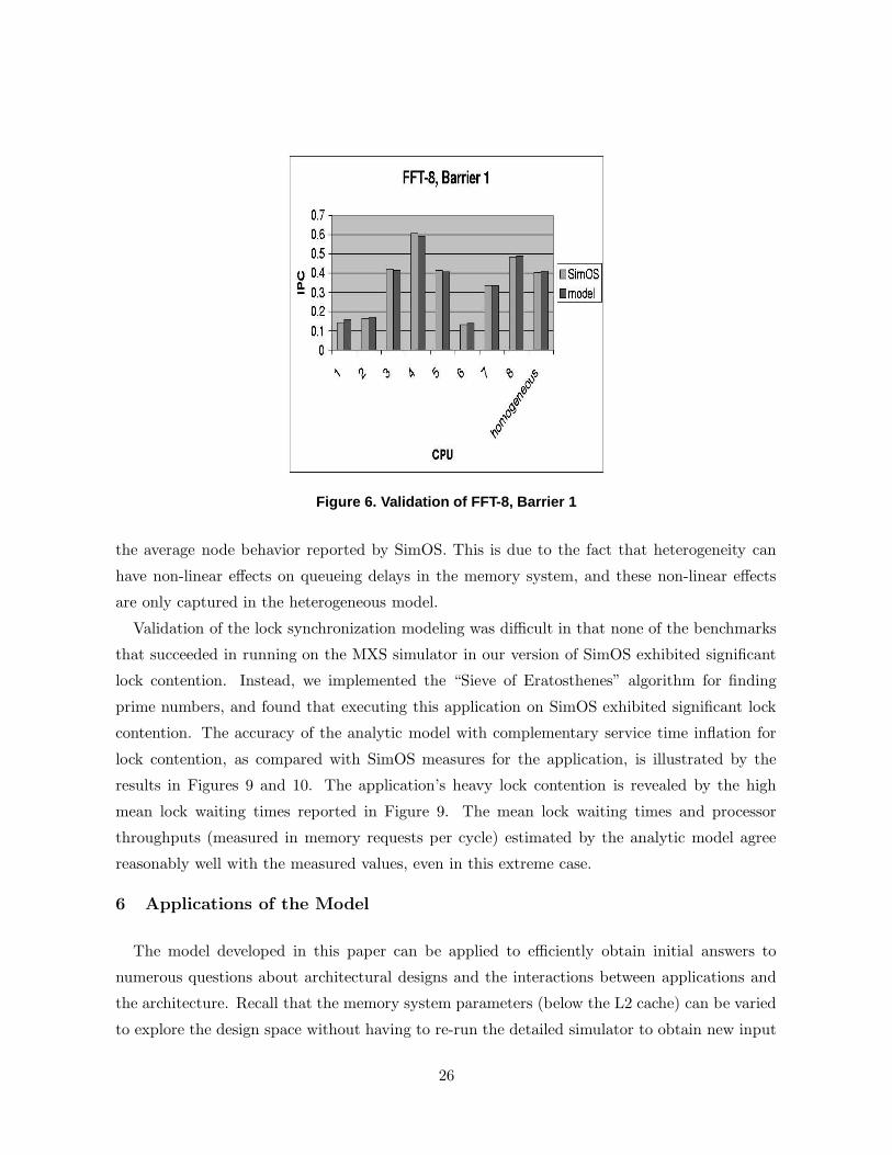
Figure 6. Validation of FFT-8, Barrier 1
the average node behavior reported by SimOS. This is due to the fact that heterogeneity can
have non-linear effects on queueing delays in the memory system, and these non-linear effects
are only captured in the heterogeneous model.
Validation of the lock synchronization modeling was difficult in that none of the benchmarks
that succeeded in running on the MXS simulator in our version of SimOS exhibited significant
lock contention. Instead, we implemented the “Sieve of Eratosthenes” algorithm for finding
prime numbers, and found that executing this application on SimOS exhibited significant lock
contention. The accuracy of the analytic model with complementary service time inflation for
lock contention, as compared with SimOS measures for the application, is illustrated by the
results in Figures 9 and 10. The application’s heavy lock contention is revealed by the high
mean lock waiting times reported in Figure 9. The mean lock waiting times and processor
throughputs (measured in memory requests per cycle) estimated by the analytic model agree
reasonably well with the measured values, even in this extreme case.
6 Applications of the Model
The model developed in this paper can be applied to efficiently obtain initial answers to
numerous questions about architectural designs and the interactions between applications and
the architecture. Recall that the memory system parameters (below the L2 cache) can be varied
to explore the design space without having to re-run the detailed simulator to obtain new input
26
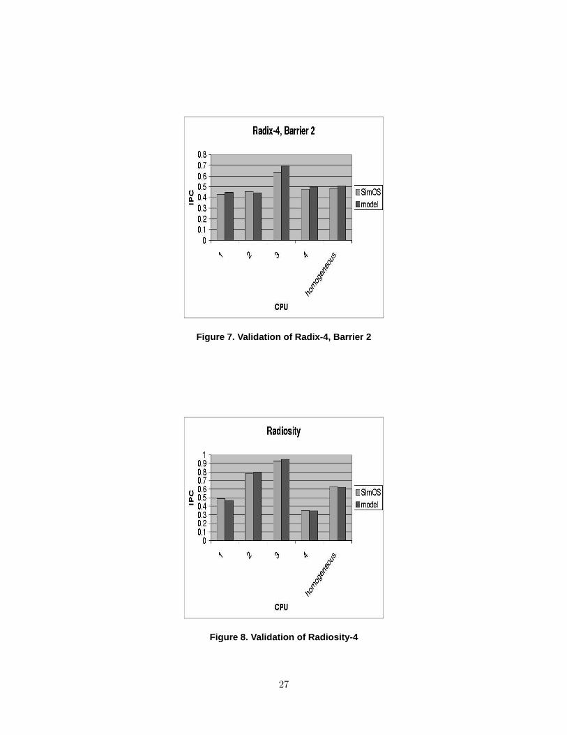
Figure 7. Validation of Radix-4, Barrier 2
Figure 8. Validation of Radiosity-4
27
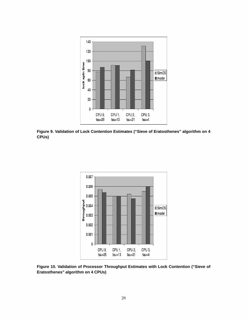
Figure 9. Validation of Lock Contention Estimates (“Sieve of Eratosthenes” algorithm on 4CPUs)
Figure 10. Validation of Processor Throughput Estimates with Lock Contention (“Sieve ofEratosthenes” algorithm on 4 CPUs)
28
parameters. The model can reveal performance bottlenecks at specific system resources due to
heterogeneous and bursty memory request traffic. This section illustrates three applications of
the model to such issues, pointing out cases in which the previous homogeneous model provides
inaccurate results.
6.1 Decoupling the Network Interface from the Directory Controller
As discussed in Section 2, the SimOS architecture requires all traffic into and out of a node
to pass through the directory controller (DC). The DC effectively assumes the responsibility of
being the network interface (NI) for all traffic, including traffic that does not require use of the
directory. This coupling of the DC and NI may, in some cases, create a bottleneck, especially as
processor speed increases relative to memory speed.
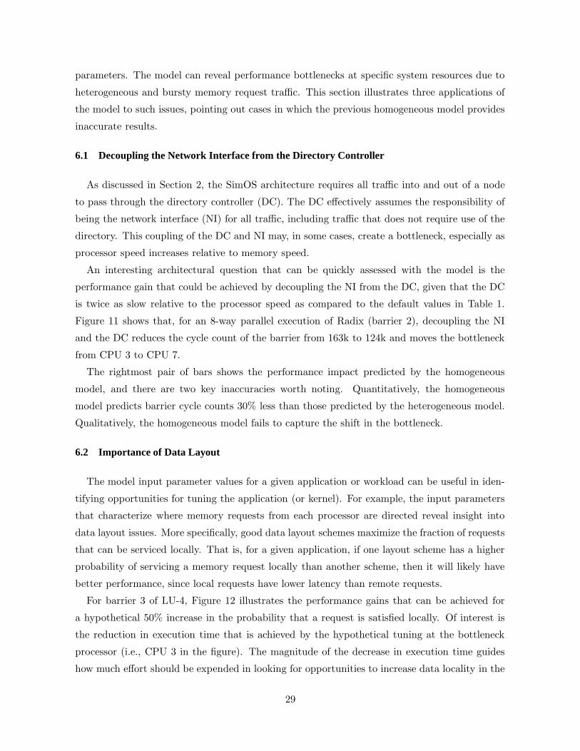
An interesting architectural question that can be quickly assessed with the model is the
performance gain that could be achieved by decoupling the NI from the DC, given that the DC
is twice as slow relative to the processor speed as compared to the default values in Table 1.
Figure 11 shows that, for an 8-way parallel execution of Radix (barrier 2), decoupling the NI
and the DC reduces the cycle count of the barrier from 163k to 124k and moves the bottleneck
from CPU 3 to CPU 7.
The rightmost pair of bars shows the performance impact predicted by the homogeneous
model, and there are two key inaccuracies worth noting. Quantitatively, the homogeneous
model predicts barrier cycle counts 30% less than those predicted by the heterogeneous model.
Qualitatively, the homogeneous model fails to capture the shift in the bottleneck.
6.2 Importance of Data Layout
The model input parameter values for a given application or workload can be useful in iden-
tifying opportunities for tuning the application (or kernel). For example, the input parameters
that characterize where memory requests from each processor are directed reveal insight into
data layout issues. More specifically, good data layout schemes maximize the fraction of requests
that can be serviced locally. That is, for a given application, if one layout scheme has a higher
probability of servicing a memory request locally than another scheme, then it will likely have
better performance, since local requests have lower latency than remote requests.
For barrier 3 of LU-4, Figure 12 illustrates the performance gains that can be achieved for
a hypothetical 50% increase in the probability that a request is satisfied locally. Of interest is
the reduction in execution time that is achieved by the hypothetical tuning at the bottleneck
processor (i.e., CPU 3 in the figure). The magnitude of the decrease in execution time guides
how much effort should be expended in looking for opportunities to increase data locality in the
29
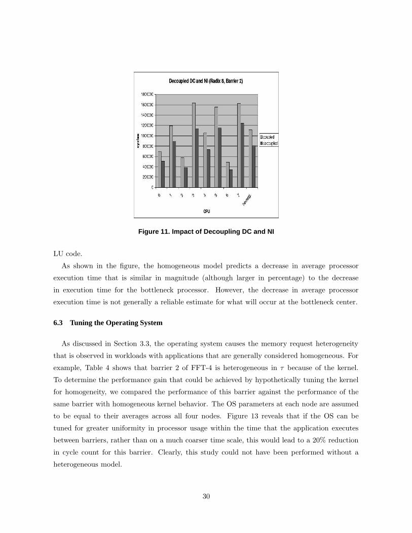
Figure 11. Impact of Decoupling DC and NI
LU code.
As shown in the figure, the homogeneous model predicts a decrease in average processor
execution time that is similar in magnitude (although larger in percentage) to the decrease
in execution time for the bottleneck processor. However, the decrease in average processor
execution time is not generally a reliable estimate for what will occur at the bottleneck center.
6.3 Tuning the Operating System
As discussed in Section 3.3, the operating system causes the memory request heterogeneity
that is observed in workloads with applications that are generally considered homogeneous. For
example, Table 4 shows that barrier 2 of FFT-4 is heterogeneous in τ because of the kernel.
To determine the performance gain that could be achieved by hypothetically tuning the kernel
for homogeneity, we compared the performance of this barrier against the performance of the
same barrier with homogeneous kernel behavior. The OS parameters at each node are assumed
to be equal to their averages across all four nodes. Figure 13 reveals that if the OS can be
tuned for greater uniformity in processor usage within the time that the application executes
between barriers, rather than on a much coarser time scale, this would lead to a 20% reduction
in cycle count for this barrier. Clearly, this study could not have been performed without a
heterogeneous model.
30
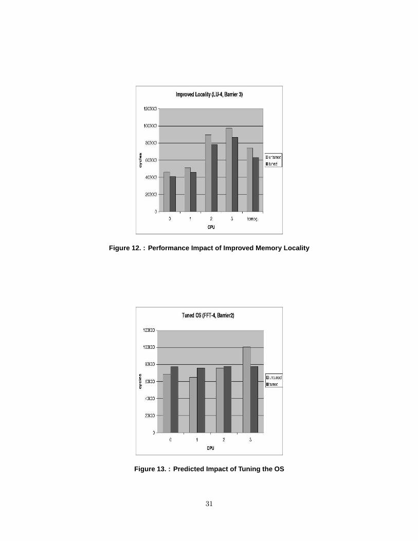
Figure 12. : Performance Impact of Improved Memory Locality
Figure 13. : Predicted Impact of Tuning the OS
31
7 Conclusions
We have developed and validated a new analytical model for evaluating the performance of
shared memory multiprocessors with ILP processors and heterogeneous processor workloads.
This work extends prior research in this area in three ways: (1) adapting and validating the
model for a different architecture than that considered in previous work, (2) modeling heteroge-
neous node behavior that was reported by SimOS even when running homogeneous applications,
and (3) applying new techniques for modeling bursty memory requests and developing techniques
for modeling lock synchronization. Despite the complexity of modeling processor heterogene-
ity and non-uniform memory access probabilities, bursty memory traffic, and lock contention,
the model converges quickly, is still several orders of magnitude faster to solve than detailed
simulation, and the number of input parameters remains manageable. The model validates
extremely well for individual processor throughput estimates, over a range of Splash-2 bench-
marks that have a wide variety of memory request behaviors, which leads to a wide range of
observed processor throughputs. Examples in Section 6 show how the model can be used to
study architectural design issues as well as to study interactions between the architecture and
the application. Moreover, the examples show that insight can be gained simply from looking
at the input parameter values that are measured for a particular workload. Model parameters
reveal application behavior and, in turn, opportunities for architectural and application opti-
mizations that target the bottlenecks revealed by the behavior (such as not enough parallelism
in the requests issued to memory).
The model is being made available for use by others in the POEMS environment [1]. The real
test of the model is how it performs in a commercial architecture design context, for which public
data is unavailable. Perhaps in making the model available to commercial systems designers,
feedback can be obtained about its accuracy in a real system design setting. Results for systems
with more nodes would also be interesting, since the model’s speed advantage over simulation
would be even greater. Future research topics also include investigating methods of coupling
the architectural model with a more abstract model of the communication and synchronization
behavior in the application.
References
[1] V. Adve, R. Bagrodia, J. Browne, E. Deelman, A. Dube, E. Houstis, J. Rice, R. Sakellariou,D. Sundaram-Stukel, P. Teller, and M. Vernon. “POEMS: End-to-end Performance Design ofLarge Parallel Adaptive Computation Systems”. IEEE Transactions on Software Engineering,26(11):1027–1048, Nov. 2000.
[2] A. Agarwal, M. Horowitz, and J. L. Hennessy. “An Analytical Cache Model”. Transactions on
Computer Systems, 7(2):184–215, May 1989.
32
[3] D. Albonesi and I. Koren. “A Mean Value Analysis Multiprocessor Model Incorporating SuperscalarProcessors and Latency Tolerating Techniques”. Int’l Journal of Parallel Programming, pages 235–263, 1996.
[4] L. A. Barroso, K. Gharachorloo, and E. Bugnion. “Memory System Characterization of CommercialWorkloads”. In Proceedings of the 25th Annual International Symposium on Computer Architecture,pages 3–14, June 1998.
[5] D. Eager, D. Sorin, and M. Vernon. “AMVA Techniques for High Service Time Variability”. InProc. ACM SIGMETRICS, pages 217–228, June 2000.
[6] D. Kroft. “Lockup-Free Instruction Fetch/Prefetch Cache Organization”. In Proc. 8th Int’l Symp.
on Computer Architecture, pages 81–87, May 1981.[7] J. Kuskin, D. Ofelt, M. Heinrich, J. Heinlein, R. Simoni, K. Gharachorloo, J. Chapin, D. Nakahira,
J. Baxter, M. Horowitz, A. Gupta, M. Rosenblum, and J. Hennessy. “The Stanford FLASH Multi-processor”. In Proc. 21st Int’l Symp. on Computer Architecture, pages 302–313, Apr. 1994.
[8] J. Laudon and D. Lenoski. “The SGI Origin: A ccNUMA Highly Scalable Server”. In Proceedingsof the 24th Annual International Symposium on Computer Architecture, pages 241–251, June 1997.
[9] E. Lazowska. “The Use of Percentiles in Modelling CPU Service Time Distributions”. In IFIP
W.G.7.3 Int’l Symp. on Computer Performance Modeling, Aug. 1977.[10] E. Lazowska, J. Zahorjan, G. Graham, and K. Sevcik. “Quantitative System Performance, Computer
System Analysis Using Queueing Network Models”. Prentice-Hall, Englewood Cliffs, NJ, May 1984.[11] M. Oskin, F. T. Chong, and M. Farrens. “HLS: Combining Statistical and Symbolic Simulation
to Guide Microprocessor Designs”. In Proceedings of the 27th Annual International Symposium onComputer Architecture, pages 71–82, June 2000.
[12] V. Pai, P. Ranganathan, and S. Adve. “RSIM Reference Manual”. Technical Report 9705, Depart-ment of Electrical and Computer Engineering, Rice University, Aug. 1997.
[13] V. S. Pai, P. Ranganathan, S. V. Adve, and T. Harton. “An Evaluation of Memory ConsistencyModels for Shared-Memory Systems with ILP Processors”. In Proc. Seventh International Con-
ference on Architectural Support for Programming Languages and Operating Systems, pages 12–23,October 1996.
[14] M. Rosenblum, S. Herrod, E. Witchel, and A. Gupta. “Complete Computer System Simulation:The SimOS Approach”. IEEE Parallel and Distributed Technology, 3(4):34–43, Winter 1995.
[15] A. Saulsbury, F. Pong, and A. Nowatzyk. “Missing the Memory Wall: The Case for Proces-sor/Memory Integration”. In Proceedings of the 23rd Annual International Symposium on Computer
Architecture, pages 90–101, May 1996.[16] D. Sorin, J. Lemon, D. Eager, and M. Vernon. “A Customized MVA Model for Shared-Memory
Systems with Heterogeneous Applications”. Technical Report 1400, Computer Sciences Dept., Univ.of Wisconsin - Madison, 1999.
[17] D. Sorin, V. Pai, S. Adve, M. Vernon, and D. Wood. “Analytic Evaluation of Shared-MemoryParallel Systems with ILP Processors”. In Proc. 25th Int’l Symp. on Computer Architecture, pages380–391, June 1998.
[18] D. Sorin, M. Vernon, V. Pai, S. Adve, and D. Wood. “A Customized MVA Model for ILP Multi-processors”. Technical Report 1369, Computer Sciences Dept., Univ. of Wisconsin - Madison, Mar.1998.
[19] V. Soundararajan, M. Heinrich, B. Verghese, K. Gharachorloo, A. Gupta, and J. Hennessy. “FlexibleUse of Memory for Replication/Migration in Cache-Coherent DSM Multiprocessors”. In Proceedingsof the 25th Annual International Symposium on Computer Architecture, pages 342–355, June 1998.
[20] B. Verghese, S. Devine, A. Gupta, and M. Rosenblum. “Operating System Support for ImprovingData Locality on CC-NUMA Compute Servers”. In Proceedings of ASPLOS VII, pages 279–289,Oct. 1996.
[21] D. Willick and D. Eager. “An Analytical Model of Multistage Interconnection Networks”. In Proc.
ACM SIGMETRICS, pages 192–202, May 1990.[22] S. J. E. Wilton and N. P. Jouppi. “CACTI: An Enhanced Cache Access and Cycle Time Model”.
IEEE Journal of Solid-State Circuits, 31(5):677–688, May 1996.
33
[23] S. Woo, M. Ohara, E. Torrie, J. Singh, and A. Gupta. “The SPLASH-2 Programs: Characterizationand Methodological Considerations”. In Proc. 22nd Int’l Symp. on Computer Architecture, pages24–36, June 1995.
34


![Distributed Shared Memory Distributed Memory[1]](https://img.pdfslide.us/doc/110x75/577d23271a28ab4e1e991e57/distributed-shared-memory-distributed-memory1.jpg)