Embed Size (px)
Citation preview

ANALYSIS ON MONEY SUPPLY, INFLATION RATE
AND ECONOMIC GROWTH THROUGH EMPIRICAL
STUDY
BY
CHAN WUN
STUDENT NO. 14200465
A PROJECT SUBMITTED IN PARTIAL FULFILLMENT OF THE REQUIRMENTS
FOR THE DEGREE OF
BACHELOR OF SOCIAL SCIENCES (HONS) DEGREE IN CHINA STUDIES
ECONOMICS CONCENTRATION
HONG KONG BAPTIST UNIVERSITY
APRIL 2016

2 | P a g e
HONG KONG BAPTIST UNIVERSITY
April 2016
We hereby recommend that the Project by Ms. Chan Wun entitled “ Analysis on
money supply, inflation rate and economic growth through empirical study” be accepted
in partial fulfillment of the requirements for the Bachelor of Social Sciences (Honours)
Degree in China Studies in Economics.
_____________________________ _____________________________
Dr. Chan Hing Lin Second Examiner
Project Supervisor

3 | P a g e
Acknowledgements
I would like to thank my supervisor Dr. Chan Hing Lin for suggesting the research topic
and guiding me through the entire study. Thanks are also due to Dr. So Pik Ki and Mr.
Chun Man Wui for their advices given.
____________________________
Student’s signature
China Studies Degree Course
(Economics Concentration)
Hong Kong Baptist University
Date : _______________________

4 | P a g e
Table of content 1. INTRODUCTION AND BACKGROUND .......................................................... 7
SITUATION OF INFLATION ................................................................................................................... 7 SITUATION OF MONEY SUPPLY .......................................................................................................... 8 SITUATION OF GDP .............................................................................................................................. 9
2. REVIEW ON THE FACT OF CHINA ............................................................. 11 SOURCES OF INFLATIONS ................................................................................................................. 11 HOW CAN THE GOVERNMENT CONTROL INFLATION? ............................................................. 13 THE CONSEQUENCES OF INFLATION ON CHINESE ECONOMY ............................................... 14 HOW CHINA PROMOTES ECONOMIC GROWTH? ........................................................................ 16 HOW DOES CHINA BALANCES INFLATION AND ECONOMIC GROWTH SIMULTANEOUSLY?
...................................................................................................................................................................... 17
3. LITERATURE REVIEW .................................................................................. 20
4. REVIEW ON THE RELATED THEORIES .................................................... 23 QUANTITY THEORY OF MONEY (QTM) ..................................................................................... 23 INVESTMENT SAVING – LIQUIDITY PREFERENCE MONEY SUPPLY (IS-LM MODEL) .. 24 AGGREGATE DEMAND – AGGREGATE SUPPLY (AD-AS MODEL) ..................................... 26
5. METHODOLOGY AND DATA ........................................................................ 28 METHODOLOGY .................................................................................................................................. 28 DATA ...................................................................................................................................................... 29
6. EMPIRICAL RESULTS .................................................................................... 31 UNIT ROOT TEST ................................................................................................................................. 31 VECTOR ERROR CORRECTION MODEL (VECM) .................................................................... 32 GRANGER CAUSALITY TEST ............................................................................................................ 35 VARIANCE DECOMPOSITION –CHOLESKY DECOMPOSITION ............................................... 39 COMPARING THE RESULTS WITH PREVIOUS RESEARCH ......................................................... 43 POLICY RECOMMENDATIONS ......................................................................................................... 44
7. CONCLUSION ................................................................................................... 45 SUMMARY OF KEY FINDINGS .......................................................................................................... 45 CONTRIBUTION AND RECOMMENDATIONS ................................................................................ 45 LIMITATIONS OF THE RESEARCH ................................................................................................... 46 A REASON FOR FURTHER RESEARCH ............................................................................................ 46
REFERENCES ......................................................................................................... 47
APPENDIX ............................................................................................................... 51

5 | P a g e
Figures and Tables
Figure 1: CPI ---------------------------------------------------------------------------------------8
Figure 2: Money supply in China ----------------------------------------------------------------9
Figure 3: GDP growth ---------------------------------------------------------------------------10
Figure 4: Impact of money supply in IS-LM model -----------------------------------------25
Figure 5: Impact of money supply in AD-AS model ----------------------------------------26
Table 1: Result of unit root test -----------------------------------------------------------------31
Table 2: Lag selection result --------------------------------------------------------------------32
Table 3: Johansen Co-integration test result --------------------------------------------------33
Table 4: VECM estimation result --------------------------------------------------------------34
Table 5: Granger causality result ---------------------------------------------------------------36
Figure 6: Variance Decomposition of LNDEFL_SA ----------------------------------------39
Figure 7: Variance Decomposition of LNM2_SA -------------------------------------------39
Figure 8: Variance Decomposition of LNGDP_SA -----------------------------------------39
Table 6: Variance Decomposition of LNDEFL_SA (in Appendix 1)---------------------51
Table 7: Variance Decomposition of LNM2_SA (in Appendix 2)-------------------------52
Table 8: Variance Decomposition of LNGDP_SA (in Appendix 3)-----------------------53

6 | P a g e
Abstract
The aim of this study is to find out the short and long run relationship among money
supply, inflation rate and economic growth in China, through empirical study from the
period of first quarter of 1999 to third quarter of 2015. Such study is important because
it directly shows the impact of monetary policy implemented by the central bank of
China (PBOC) and illustrates a direction for the future monetary policy. This research
was carried out by the approaches of Vector Error Correction Model (VECM), Johansen
co-integration test, Granger causality and variance decomposition. This research
produced a number of key findings: one co-integration equation among the three
variables, thus implied that a long run relationship exists among money supply growth,
inflation rate and economic growth in China; a bi-directional causality between money
supply growth and inflation rate were found in the short run; money supply growth and
inflation rate do granger causes of economic growth while economic growth does not
granger cause of money supply growth and inflation rate. It is therefore concluded that
the government should control money supply to balance inflation and economic
development. On the one hand, the government of China should implement a relatively
tight monetary policy. On the other hand, lagged effects of tight monetary policy may
lead to economic recession. Therefore, it is recommended that the government of China
should take measures to closely monitor the growth rate of the money supply. In
particular, cautious regulation should be implemented for the macroeconomic policy in
order to avoid financial risks.

7 | P a g e
1. Introduction and Background
Situation of inflation
China, growing rapidly since its open and reform in 1978, creates a new record
regarding to her GDP growth. By using GDP per capita at current price level, China
doubles her GDP per capita in 5 years while Japan and United States spent 27 years and
20 years respectively.
Meanwhile, what economists are always concern that whether high economic growth
compounded with high inflation rate. Tong and Zhao (1996) stated that after 15 years of
economic reforms, the most notable feature of today's Chinese economy is high
economic growth compounded with high inflation.
Inflation has a curial influence on China. Given the fact that CPI boosted from 98.3 in
Jan 2009 to 106.4 in Jan 2011, it climbed to second high level after year 2008.1 Since
China’s reform and opening up, a number of economically underprivileged are still
situated nationwide, inland especially, and would suffer if the price level keep
increasing, as a result of higher living expenses. Inflation would offset most of their
saving and earning. The issue of inflation in China definitely deserves a closer look.
1 See figure 1.

8 | P a g e
Situation of money supply
Friedman M. (1963) stated that high money supply led to high inflation in the long-term,
but there are non-regular relations between money supply and inflation in a short-term.
According to People Bank of China (PBOC), the average growth rate of M1 and M2
was 14.7% and 16.4% respectively from 2000 to 2015. The below graph shows that the
quantity of M2 raised from RMB45.3 trillion on September 2008 to RMB 85.7 trillion
in October 2009, the monthly growth rate of it increased from 15.3% to 29.4%
respectively, which was the highest rate over the past years; the quantity of M1 raised
from RMB15.6 trillion on September 2008 to RMB 20.2 trillion on October 2009, the
monthly growth rate increased sharply from 9.4% to 32%.2 The main reason behind is
due to the government’s “Chinese economic stimulus program” implemented from the
period of 2008 to 2010.3 The government launched a “4 trillion plan” in order to avert
2 See figure 2.
3 The government of China responded quickly after 2008 global financial crisis and strongly by announcing a stimulus package of US$586 billion over two years or 13.4% of GDP as reported
by the World Bank in its report, Infra update, June 2010: Supporting China’s infrastructure
stimulus under the infra platform. (P.1)
9698
100102104106108110
19
99
Y1
2M
20
00
Y6
M
20
00
Y1
2M
20
01
Y6
M
20
01
Y1
2M
20
02
Y6
M
20
02
Y1
2M
20
03
Y6
M
20
03
Y1
2M
20
04
Y6
M
20
04
Y1
2M
20
05
Y6
M
20
05
Y1
2M
20
06
Y6
M
20
06
Y1
2M
20
07
Y6
M
20
07
Y1
2M
20
08
Y6
M
20
08
Y1
2M
20
09
Y6
M
20
09
Y1
2M
20
10
Y6
M
20
10
Y1
2M
20
11
Y6
M
20
11
Y1
2M
20
12
Y6
M
20
12
Y1
2M
20
13
Y6
M
20
13
Y1
2M
20
14
Y6
M
20
14
Y1
2M
20
15
Y6
M
20
15
Y1
2M
Figure 1: CPI (The same month last year=100)

9 | P a g e
an economic recession induced by the global financial crisis. The details would be
discussed in the next section.
Situation of GDP
China’s GDP per capita rose from approximately USD180 in 1979 to approximately
USD7, 600 in 2014, which was up around 40-fold. Although, the GDP per capita of
China is still at a very low level comparing with developed countries, such an
exceptionally fast growth of its economy for a long period of time always attracts the
attention from all over the world, deserving us to study the Chinese economy.
After all, a decreasing growth rate of GDP from 19% to 8% has been recorded between
2008 to 2009, and then climbed up to 18% in 2010 as shown in the below graph.4 It
was almost the lowest growth rate since China was opened up in late 1970’s. It was
believed that both global financial crisis and monetary policy contributed to the
economic fluctuation. Implying the monetary policy does affect the economic growth,
however, the real impact on output growth is still an uncertain issue.
4 See figure 3.
05
10152025303540
19
99
Y1
2M
20
00
Y7
M
20
01
Y2
M
20
01
Y9
M
20
02
Y4
M
20
02
Y1
1M
20
03
Y6
M
20
04
Y1
M
20
04
Y8
M
20
05
Y3
M
20
05
Y1
0M
20
06
Y5
M
20
06
Y1
2M
20
07
Y7
M
20
08
Y2
M
20
08
Y9
M
20
09
Y4
M
20
09
Y1
1M
20
10
Y6
M
20
11
Y1
M
20
11
Y8
M
20
12
Y3
M
20
12
Y1
0M
20
13
Y5
M
20
13
Y1
2M
20
14
Y7
M
20
15
Y2
M
20
15
Y9
M
%
M1 M2

10 | P a g e
This study is intended to employ Vector Error Correction Model (VECM) to analyze the
correlations of money supply, inflation rate and economic growth in both short run and
long run perspectives. Though different economists conducted similar studies before,
this paper still contains a number of contributions. Firstly, previous studies only covered
periods up to 2007, and this study cover the period of 1999 to 2015. Extending the study
to recent years is important because there are probably changes in the situation after
2008 global financial crisis. Secondly, many previous researches have tended to focus
on explaining the relationship between money supply and economic growth. Yet, this
paper is to analyze the how the PBOC can utilize the monetary policy to balance the
economy development and inflation rate, which is useful to understand the rationale
behind monetary policy that the government of China implements as well as provides
further policy recommendation.
In the followings, this paper will be divided into different sections: (2) a review on the
fact of China; (3) a literature review is to present summarizing contributions from
previous studies; (4) a review on the related theory; (5) an explanation of methodology
and the sources of data used; (6) an analysis of the empirical results; and (7) the
concluding section.
0%
5%
10%
15%
20%
25%
2000 2001 2002 2003 2004 2005 2006 2007 2008 2009 2010 2011 2012 2013 2014
Year
Figure 3: GDP Growth

11 | P a g e
2. Review on the fact of China
Sources of inflations
In recent years, the continuous rises in price level accompany with the economic growth
of China. Inflationary pressures are getting more serious as economic develops more
rapidly. China’s economy constantly expand in the few decades, while the domestic
supply of many types of primary commodities is far behind its demand, shortage and
inefficiency have been noted. As a result, the rising demand of import goods increases
their import prices, directly contributing to the general price level. Besides, since
developed countries always injected money into their economy for recover the economy
from the global financial crisis. Due to the time lag effect, it increases price level in the
nearly future. The increasing money supply flows into both of the goods and financial
markets of China, leading to sharp rises in the price of substantial merchandise,
including energy, precious metals and grain. It will continue to increase imported
inflation expectations.
Moreover, cost-push pressure on price level is the second source of inflation. Crude oil
and metal ore are the common raw materials of many productions, such as energy
industries, logistics and manufacturing for production. By price transmission, the input
price will cause the price of final product to rise further. With the producer price index
(PPI) gradually picked up, part of it will transfer to the consumer price index (CPI).
Therefore, change in crude oil price and metal ore are the second important factors that
contribute to the inflation. If the prices of these two categories increased sharply, there
would be a significant impact on the overall price level. Thus, their impact cannot be
neglected.
12 | P a g e
Jing and Wong (2006) employed co-integration analysis to investigate the prices of
wholesale grain and consumer price level (CPI) from 2001 to 2005 in China, and found
that grain price exerts Grange causality on inflation in the long run, but the effect is
weak in short run. That is to say, change in the price of grain does have a strong
influence on CPI in the long run.
Furthermore, many industries in China rely highly on the agriculture industry,
especially light and tertiary industries. Therefore, if there is a large fluctuation in price
of agricultural products, the production costs and final product prices of various
industries will suffer from it. According to the research of Liu Yuanchun (2015), the
degree of dependence of end-product production on agriculture sector was 2.05, which
reflected that the dependence coefficient of the agricultural sector was twice that of the
average level.5 This implied that most industries have a very high dependence on the
sector. Therefore, changes in agricultural product prices would inevitably result in a
high degree of impact.
To conclude, imported inflation is the main source of inflation while cost-push inflation
is the second source of inflation. Meanwhile, agricultural products have the widest
scope of impact that affecting light industries and service industries such as
accommodation and catering services. On the contrary, the impact of oil and natural gas
are more concentrated in energy and heavy industries.
5 The dependence coefficient reflects the degree of dependence of end-product production on a certain sector.

13 | P a g e
How can the government control inflation?
As the second largest and the fastest growing economy of the world, China performs a
unique socialist open market economy. The prices are tightly controlled by the
government, yet remains open to free market forces. Hence, whenever the economy is
experiencing inflationary gap, monetary policy and fiscal policy can be the tools for the
government to restore the economy into a relatively full employment level. The slower
growth will then lead to lower price level.
In China, the government mainly utilizes monetary policy to achieve the goals. The
People’s Bank of China (PBOC) is the central bank of China who formulates and
implements monetary policy in order to maintain the stability of the currency and
safeguard financial stability, and thereby promote economic growth. In 2016, the PBOC
targets inflation rate at 4.0%, which is relatively high comparing with most of the
countries in the world. For instance, Federal Reserve, Bank of England Bank of Japan
and Bank of Korea target on 2% of inflation rate.
The major instruments of monetary policy including open market operation, reserve
requirement ratio and interest rate or discount rate. Firstly, the PBOC uses open market
to purchase or print yuan as needed to increase the money supply, though this can lead
to high inflation. However, China has tight state-dominated controls on its economy and
the government to control inflation differently than in other capitalist countries. The
government of China can make use of subsidies and other price-control measures to
manipulate the price level as state-owned enterprises (SOEs) still take a significant role
on many sectors, like natural resource, industry, medical and railway industries.

14 | P a g e
Secondly, the required reserve ratio is the proportion that commercial banks are
required to keep a certain amount of their total deposit with the PBOC. When the PBOC
reduces the reserve ratio, commercial banks keep less of their deposit as reserve, which
implies that there are more money available for the bank to lead, increasing in money
supply and lead to a higher inflation, and vice versa.
Thirdly, discount rate (or interest rate) is a major tool central bank always uses to
control the inflation rate of an economy. Whenever commercial banks borrow loans
from the central bank, interest would be charged on such of the borrowing, which is
considered as discount rate. PBOC can change the discount rate to increase or decrease
the cost of borrowing of each borrowing, which affect the availability of money in open
markets and affect the price level eventually. In 2011, the CPI reached around 105,
which was the second high level after 2000. The PBOC announced to raise the discount
rate to 6.31% in April 2011, in order to suppress the high inflation rate.
The consequences of inflation on Chinese economy
In 2010, the president Hu Jintao warned his colleagues to be "more active in dealing
with the relationship between stable economic growth, adjusting the economic structure
and managing forecasted inflation". This showed that management of inflation rate was
one of the most important tasks of the central bank in the sense that persistently high
inflation could hurt the economy and generate other social consequences.
Inflation is a sustained increase in the general price level of goods and services in an
economy over a period of time. There are several consequences that inflation would

15 | P a g e
bring about, including fall in wealth, investment, exchange rate, GDP and income
redistribution.
A rise in the price level means that using the same amount of money can buy fewer
goods or services. That is, inflation causes fall in the purchasing power of money. As a
result, this explains why, during the period of inflation, Chinese citizens often choose to
invest their wealth into physical assets, like real estate, rather than keep it in a monetary
form in the bank in order to shelter the wealth of individual from inflation.
Unexpected inflation redistributes income among groups in the society. It occurs as
wages and salaries of a party increase quickly than the price level while the wages and
salaries of another party increase slowly than the price level. Debtors gain as they repay
creditors with money that are worth less in terms of purchasing power. Another
example is tenant pays a fixed amount of money to the landlord as they have signed a
contract before inflation appears. After inflation arises, the landlords suffer while the
tenants gain.
Experiencing high rates of inflation affects the exchange rate and the foreign trade. As
inflation pushes up the price of the domestic products, if the exchange rate remains
unchanged. China's domestic products will be less competitive internationally, and the
demand for export drops. On the other sides, import rises as it becomes relatively
cheaper in term of renminbi (RMB). Consequently, it leads to decrease in the net export,
current account and the balance of payments may deteriorate, which directly reduce the
GDP of China. According to the statistics of trading economics, in 2015 as a whole,
China’s total trade dropped by 8 percent, as exports shrank 2.8 percent due to a weaker
RMB and falling commodity prices.

16 | P a g e
Companies respond unfavorably to inflation as it causes uncertainty and fall in
investment. It is because it will suppress consumer spending and reduces aggregate
demand. Inflation also increases costs and reduces the competitiveness of products. All
in all, falling in aggregate demand is likely to compel companies to postpone their
capital investment.
Gorrie (2013) wrote that Chinese real estate boomed as China’s stimulus monetary
policy has released inflationary forces throughout the country.6 But that
stimulus-derived inflation was mostly transmitted through rising asset price rather than
goods price, therefore the inflation was not felt by consumers at the beginning, but
rather by higher price in real estate development projects.
How China promotes economic growth?
In this part, the 2008-2009 Chinese economic stimulates policy would be mainly
discussed. By reviewing policy the government of China implement, it would be able to
understand how China government promotes its economic growth or prevent suffering
from the global financial crisis.
China did a lot to intervene the market after 2008 global financial crisis. China invested
4 trillion yuan (US$586 billion) stimulus package in infrastructure and social welfare, to
prevent the country from the global downturn. Of the package, 29% came from central
government spending, with the rest from local governments (31%) and bank’s lending
(40%).
6 Gorrie (2013), p.156.

17 | P a g e
In June 2009, the World Bank raised the GDP growth prediction of China for 2009 from
6.5% to 7.2%, which signaled that China would do better than the world expected. Not
surprisingly, China did do better than the rest of the world after the 2008 global
financial crisis. The GDP growth for 2009 was 8%, which was even better than the
World Bank expected. Many economists believed that it has been helped by the
stimulus package while some did not agree as it brought out other serious problems to
the society, like inflation and non-performed loans.
According to the report of World Bank in 2010, there was more than a third of the
stimulus allocated to infrastructure sectors, including roads, railways and grids. For
example, US$300 million was approved to NanGuang railway and GuiGuang railway
projects respectively. The government mainly focused on the mega-projects, primarily
on large-scale infrastructure as well as the reconstruction effort for post-earthquake
Sichuan, for example, US$710 million was approved to Wenchuan earthquake recovery
project. Low carbon infrastructure was also prioritized, with 8000 km of high-speed
railway lines and grid modernization projects receiving significant allocations.
How does China balances inflation and economic growth simultaneously?
As we can see in the above illustration, the expansionary monetary policy is likely to
cause high inflation and also high economic output, while the contractionary monetary
policy is likely to cause low inflation and also low economic output. It is therefore
difficult for the government to achieve low inflation rate and high economic growth
simultaneously.

18 | P a g e
In 2004, the world economy recovered in an all-round way. The PBOC implemented a
sound monetary policy.7 China’s GDP increased by 9.5% to 13.7 trillion yuan. M2
grew by 14.6% by year to 25.3 trillion yuan at the end of 2004. However, inflation has
not eased fundamentally since agriculture has yet to strengthen its fundamental role in
the economy, pressure still looms large for a rebound of fixed-assets investment. The
government noticed that the effectiveness of monetary policy needed to be enhanced
and the stability of the financial sector needs to be strengthened. Therefore, in 2005, the
PBOC kept continually to pursue the sound monetary policy. Measures had been taken
to support steady economic development as well as to prevent inflation and systemic
financial risks, such as used the interest rate leverage to promote balanced development
of economic aggregates and structural adjustment.
In the middle of 2008, as the global financial crisis spread and deepened, national
macroeconomic policy underwent substantial changes, the PBOC adjusted the intensity
of monetary policy in timely manner in order to maintain stable and relatively rapid
economic growth and prevent price hikes. A “4 trillion yuan stimulate economic plan”
launched, and to guide financial institutions to increase credit lending to agriculture,
rural areas, small- and medium-sized enterprises and post-disater reconstruction on a
preferential basis. The PBOC adopted moderately loose monetary policy to recover the
economy and stabilize market confidence. At the end of 2008, M2 increase 17.8%
posted 47.5 trillion yuan. GDP was 30.1 trillion yuan, rose 9% by year, and the CPI
grew 5.9% by year.
The meeting of the Central Economic Work Conference in December 2010 determined
the “strengthen and improve macroeconomic regulation to maintain stable and healthy
7 Stability, continuity and forward-looking manner will characterize the sound monetary policy
implementation.

19 | P a g e
economy” economic work in 2011. Undoubtedly, the effective control of inflation has
become the primary goal of the 2011 macro-control policies. To this end, moderately
loose monetary policy has been gradually shifted to sound monetary policy. From the
end of 2010 to 2011, the PBOC has raised the deposit reserve ratio eight times and
raised interest rates four times in order to control prices. After the CPI rose in January
2011 again, the urgency and necessity of the implementation of such a policy was even
more prominent. The central bank’s decision to immediate raise the deposit reserve ratio
fully demonstrated this point.
According to People’s Bank of China branch president of Qingdao city center Xin
(2013), he stated that over year of 2012, China’s adherence to the idea of “steady
progressive” economic development, inflation has been effectively controlled, but also
inevitably the economic slowdown and the tightening real capital in economy.
In 2014, the PBOC has continued with a sound monetary policy. The PBOC also
asymmetrically lowered the benchmark lending and deposit interest rates and increased
the flexibility of the interest rates for open market operations to reduce the financing
costs for the whole society. At the end of 2014, M2 was up 12.2% by year. GDP growth
was 7.4% by year and the CPI was up 2.0% by year. Consumer prices picked up
moderately, while employment remained stable.
Under the PBOC, the objective of China’s monetary policy is to maintain a stable
currency and thereby promote economic growth. But in fact, in practice, the monetary
policy is also concerned about full employment and balance of payments. In the process
of macro-control policy-making, it is needed to handle the relationship among the
currency, economic growth, inflation and balance of payments, especially the
relationship between inflation and economic growth.

20 | P a g e
3. Literature Review
Most early studies investigated the relationship among various variables, especially
money growth, inflation rate and economic growth. The Quantity Theory of Money
(QTM) suggests that quantity of money determines the value of money. Henry
Thornton (1802) believed that more money equals more inflation and that an increase in
money supply does not often cause an increase in economic output.
Tobin and Clower (1970) found that change in money supply would affect the short run
economic output though empirical study. The studies of Stock and Watson (1989) and
Cover (1992) also found out the same conclusion. Furthermore, McCandless and Weber
(1992) through observed the output growth rate, average inflation rate and money
supply growth of the recent 30-year among 110 countries, then concluded that there is
no correlation between growth rate of money and real output in the long run.
The recent rush of publications in the area may give rise to the importance of inflation.
Mishra et al. (2010) completed a study on the relationship among money, price, and
output in developing countries, particularly in India. The data of money supply, price
level and output were investigated from the period of 1950 to 2009 by using vector error
correlation model and co-integration test. In the long run, bidirectional causality was
found between output and money supply. In the short run, bidirectional causality was
also found between money supply and price level. Yet in the long run, a unidirectional
causality resulted from price level to money supply and from price level to output.
In Sudan, Ahmed & Suliman (2011) examined three macroeconomic variables (real
gross domestic product, money supply and price level (CPI) of annual data from the
period of 1960 to 2005. The Granger causality test result shows that money supply has a

21 | P a g e
direct effect on the price level of products, however, there was no causality exits
between money supply and economic growth.
When it comes to the case of China, Huang and Deng (2000) examined the data of
money supply and output growth from the period of 1980 to 1997. They argued that
money supply was non-neutral to the output. It implied that the money supply was still
playing a significant role in the economy operation of China. Bin Liu (2001) observed
the effect of monetary policy on consumption and investment by Vector Autoregression
model (VAR model) and emphasized that the money supply would affect the output in
the short term, but not in the long run.
Wong and Li (2004) concluded that the basic reason for the inflation in China is the
excessive money supply. They reconfirmed the real effect of monetary policy is mainly
reflected on the economic growth, and both money demand and interest rate are weak
exogenous variables for the co-integrating vector by employing stochastic
co-integration and short run Granger causality.
Liu and Jin (2005) found that the increase in money supply did not necessarily stimulate
inflation in the long run as the change in money supply had been absorbed by the
economy in the process of monetization. Moreover, they concluded that money supply
and economic growth boost each other, and inflation hinders economic growth in the
long run.
Yao (2007) examined the relationship among money supply, inflation and economic
growth by employing co-integration and variance decomposition approach. It confirmed
money supply was exogenous and non-neutral to the output in the long run, and found
out that inflation rate and economic growth have negative relationship in the short run

22 | P a g e
and long run, but they would fall back to natural level. Moreover, they showed that the
money supply has lag effect on inflation rate and economic growth.
Xie, Tang and Cui (2009) analyzed on the relationship among money supply, economic
growth and inflation in China from 1998 to 2007 by using the approaches of
co-integration and Granger causality test. They concluded that a new source of
stimulating economic growth should be sought other than using loose monetary policy
since the finding told that there is no co-integration relationship between money supply
and economic growth.
To sum up, empirical analyses showed that, there was a great uncertainty between the
relationship of money supply and economic growth, and there was no clearly defined
relationship between the money supply and economic growth so far. It seems that
further investigations are needed in order to examine the correlation of these three
variables (money supply, inflation rate and economic growth).
From the literature review above, we can see that these conclusions of different studies
are not consistent. This phenomenon is mainly due to the choice of sample spacing and
modeling methods. The effects of supplying more money remain complex to policy
makers. Darrat and Dickens (1999) found that the relationship of money and economic
performance are complicated, as a result, applying multiple-linear regression was
reasonable than simple linear regression, and gathering more samples was also better.
Therefore, this paper utilizes the data of first quarter of 1999 to third quarter of 2015
from China to establish the relationship among money supply, inflation rate and
economic growth by using Vector Error Correction Model (VECM), Johansen
co-integration test as well as Granger causality test.

23 | P a g e
4. Review on the related theories
Before developing the time series regression model, this paper would like to review the
related theories that based on the knowledge learned before. QTM, LM-LS model and
AD-AS model are employed in this section. After, a regression model would be
developed.
Quantity Theory of Money (QTM)
Quantity theory of money (QTM) is a relationship among money, output and prices that
is used to study inflation. It is supported and calculated by using the Fisher Equation on
Quantity Theory of Money.
𝑀𝑉 = 𝑃𝑌 (1)
Each variable denotes the following:
𝑀 = Money supply
𝑉 = Velocity of money / circulation
𝑃 = Average price level
𝑌 = Real aggregate output
The QTM assumes that only V is fixed in the short run. Therefore, equation (1) can be
rewritten as %∆𝑀 = %∆𝑃 + %∆𝑌. It implies that any change in money supply will
affect the nominal GDP (𝑃𝑌). As a result, monetarists view control of the money
supply as the key variable in stabilizing the economy.

24 | P a g e
The QTM also assumes that V and Y are constant in the long run. Therefore, equation
(1) can be rewritten as %∆𝑀 = %∆𝑃, means that if the amount of money in an
economy goes up by 20%, price level will also goes up by 20%. The consumer therefore
needs to spend 20% more for purchasing the same amount of the good or service. It
implies that in the long run, changes in the money supply only cause change in the price
level. This conclusion explains Friedman's famous quote "Inflation is always and
everywhere a monetary phenomenon." The fact that changes in the money supply have
no long-run effect on real variables is called the long-run neutrality of money.
However, many economists, like J. M. Keynes, hold a different view as they believe
that the velocity of money does not remain constant over time. Moreover, according to
them, the theory fails in the short run when the price is sticky. As a result, LS-LM and
AD-AS models would be discussed in the following.
Investment Saving – Liquidity Preference Money Supply (IS-LM model)
John Hicks (1937) gave birth to the LS-LM model. It is a short run macroeconomic
model that graphically represents the interaction between two equilibrium markets
given that price is fixed in the short-term. The IS curve represents the every equilibrium
point of the goods market while LM curve represents every equilibrium point of the
financial market. Goods and financial markets joint together to determinate the out and
interest rate in the short run. The interest rate affects output through investment and
output affects the interest rate through money demand.
Equation (2) is the IS equation in the goods market. It states that the condition for
equilibrium requires the supply of goods (YY) be equal to the demand for goods (ZZ).

25 | P a g e
𝑌𝑌 = 𝑍𝑍 = 𝐶(𝑌 − 𝑇) + 𝐼(𝑌, 𝑖) + 𝐺 (2)
Equation (3) is the LM equation in the financial market. It states that the condition for
equilibrium requires the real money supply is equal to real money demand, which
depends on real income, Y, and the interest rate 𝑖.
𝑀
𝑃= 𝑌𝐿(𝑖) (3)
Therefore, the negative relationship between interest rate and output is known as the IS
curve, and the positive relationship between interest rate and output is known as the LM
curve.
Figure 4: Impact of money supply in IS-LM model
When the government implements monetary expansion, the result is showed in the
figure 4. Monetary expansion, for instance, increase money supply, causes the LM
curve to the right (LMLM’) and IS curve remains unchanged because money supply
does not affect the equilibrium of the goods market. In equilibrium, output increases
(𝑦0 → 𝑦1) and interest rate decreases (𝑖0 → 𝑖1) given that price is fixed in the short
run. It implies that an increase in money supply affects the real output in the short run
given price is sticky, but the effect of real output still remain uncertain in the long run
situation. The conclusion is consistent with QTM.

26 | P a g e
Aggregate Demand – Aggregate Supply (AD-AS model)
AD-AS model is based on the theory of Keynes (1936) put forward in his work The
General Theory of Employment, Interest, and Money. It helps to explain price level and
output through the relationship of aggregate demand and aggregate supply. The model
consists of three curves including the aggregate demand curve (AD), the short-run
aggregate supply curve (SAS) and the long-run aggregate supply (LRAS).
Aggregate demand is the total amount of the goods and services demanded at different
price level.8 Aggregate supply is the total amount of goods and services in the economy
available at all possible price level.9 Long-run aggregate supply is the total output of an
economy at the full employment level.10 There are differences between long run and
short run aggregate supply because price may not able to adjust freely to clear the
market and there are no misperceptions about the price level in the long run.
Figure 5: Impact of money supply in AD-AS model
8 AD curve is downward sloping. Since there are wealth, interest rate and exchange rate effects,
when the price level rises, the quantity of output demanded falls. 9 AS curve is upward sloping as the quantity of output supplied rises when the price level rises. 10 LRAS curve is vertical at the potential output as the potential output is determined by the
resources (labour, capital and natural resources) and technology available, and is not affected by
the price level.

27 | P a g e
The result of expansionary monetary policy is illustrated in figure 5. Supposes the
economy starts at point A where price level is 𝑃1 and aggregate output equal to the
potential out 𝑌𝐹. In the short run, when the government increases money supply, AD
curve shifts to the right, the economy will adjust to point B along the SAS. The price
level will increase to 𝑃2, and aggregate output will fall to 𝑌2.11
In the long run, prices are no longer rigid. Besides, wages can fully adjust upward to
raise the cost. Also, misperceptions about the price level will be corrected, the expected
price level will increase. The SAS curve will shift leftward to 𝑆𝐴𝑆2, and the short-run
equilibrium point will shift to point C. The aggregate output will return to the potential
output (𝑌𝐹), the price level will further increase to 𝑃3, and the long-run equilibrium is
attained.
To conclude, increases in money supply would increase the price level in the short run
and/or further increase the price level in long run. Furthermore, increases in money
supply would increase output level in short run, but there is no change in the long run.
The result is similar to QTM and LS-LM model.
11 The possible reasons for the simultaneous raise in the price level and aggregate output in the short run are sticky-price, sticky-wage and misperceptions theories.

28 | P a g e
5. Methodology and Data
Methodology
The ultimate goal of this paper is to investigate the correlations of real money supply,
inflation rate and real gross domestic product. Since the three data sets show there were
non-stationary, which violate the OLS assumption. Therefore, vector error correction
model was used for the examination. Both long run and short run relationships would be
established to illustrate if there are any relationships among the above three variables.
Eviews 8.0 was employed for estimating the system.
Money supply M2 would be used instead of M1, since it is a broader term when
comparing with M1. China money supply M2 includes M1 plus short-term time
deposits and lending in banks. Thus, it would be a better indicator to reflect the effect of
monetary supply controlled by the government.
Besides, many previous researches used the CPI to calculate the real GDP. However, it
could generate a large error between the true value and measured value of real GDP.
Since CPI can only represent the common basket resident always purchase in the market
but it is not a general indicator of all the goods and services in a country. Instead of
using CPI, this paper would adopt GDP deflator to derive the real GDP in China, and
also used it to represent the price level.
Furthermore, seasonal adjustment X12 is used in order to eliminate the seasonality of
the data.12 Finally, all the variables are taken logarithm after seasonal adjustment. LN
12 The seasonal influence is removed from that particular time series, the data can be
meaningfully compared across different quarter and predictions for the future can be accurately
forecast.

29 | P a g e
would be added before the variables to represent natural logarithm form; the D before
the variables represent they are at the first differenced.
Error Correction Model (ecm)
∆𝑦𝑡 = 𝛼𝑒𝑐𝑚𝑡−1 + ∑ Γ𝑖𝑝−1𝑡=1 Δ𝑦𝑡−1 + 𝜀𝑡 (4)
Where ∆𝑦𝑡 is the dependent variable vector at first differenced; 𝑒𝑐𝑚𝑡−1 is error
correction term, it reflects the long-run equilibrium relationship between variables; the
coefficient vector 𝛼 reflects the adjustment efforts when there is disequilibrium
between the variables and its long-run equilibrium; 𝑝 is the lag length; 𝜀𝑡 is
disturbance vector or error term. All of the coefficients of differential term of
independent variables reflect the short-run fluctuations of the variables as the effect of
short-run change of dependent variables.
Data
By obtaining the data of M2, nominal GDP, and GDP index from 1999 to 2015 from
National Bureau of Statistics of the People’s Republic of China, the calculation process
shown as the following:
(1) Divided real GDP in current year by GDP index to calculate the real GDP in the
previous year; (2) then divided the nominal GDP by the real GDP at the same year to
calculate the GDP deflator; (3) adding the monthly-based data of M2 to find out the
quarterly based data of M2; (4) divided the quarterly based M2 by the GDP deflator to
find the real M2.

30 | P a g e
The final data set of M2, GDP deflator and real GDP are using quarterly based and 2010
as the base year.

31 | P a g e
6. Empirical Results
Unit root test
Unit root test will be employed before run a time series regression analysis to check
whether the variables are stationary or not. Since if the variables are not stationary, the
use of OLS will produce spurious regression. This paper used Augmented Dickey-
Fuller (ADF) to test the unit root of 𝐿𝑁𝑑𝑒𝑓𝑙_𝑠𝑎, 𝐿𝑁𝑚2_𝑠𝑎 and 𝐿𝑁𝑔𝑑𝑝_𝑠𝑎 and the
first differenced of them. The result of unit root test is shown in Table 1 in the
following.
Table 1. Result of unit root test
Variable
Test form
(C, T, K) ADF
test stat. Prob. Variable
Test form
(C, T, K) ADF
test stat. Prob.
LNdefl_sa (C,T,1) -1.913803 0.6360 DLNdefl_sa (C,T,0) -3.630396 0.0349** LNm2_sa (C,0,1) -0.139974 0.9400 DLNm2_sa (C,T,0) -4.52116 0.0030**
LNgdp_sa (C,T,1) 0.123241 0.9969 DLNgdp_sa (C,T,0) -6.658482 0.0000**
Notes: The test form (C, T, K) represents unit root test equation, including constant term, trend and lag length respectively. ** denote reject the null hypothesis at the 5% significant level.
From Table 1, the p value of 𝐿𝑁𝑑𝑒𝑓𝑙_𝑠𝑎, 𝐿𝑁𝑚2_𝑠𝑎 and 𝐿𝑁𝑔𝑑𝑝_𝑠𝑎 are larger than
5%, which represent they do not reject the null hypothesis.13 It shows that the variables
are not stationary or have unit root. Thus, the data cannot be applied for the
co-integration test. Though when the variables are converted to the first differenced,
which means 𝐷𝐿𝑁𝑑𝑒𝑓𝑙_𝑠𝑎, 𝐷𝐿𝑁𝑚2_𝑠𝑎 and 𝐷𝐿𝑁𝑔𝑑𝑝_𝑠𝑎 , it shows that the p value
of them, are smaller than 5%. It means that the variables are stationary or do not have
unit root at their first differenced. As a result, co-integration test can be employed to
check if the variables have co-integration relationship.
13 Null hypothesis 𝐻0 stated that the variable is not stationary or have unit root.

32 | P a g e
Vector Error Correction Model (VECM)
To develop a VECM, here are three steps involved. First of all, lag selection is needed
to confirm how many lag to choose toward the model. Secondly, Johansen
co-integration test is needed to confirm how many relationships the variables have. Last
but not least, VECM could be developed.
1. Lag selection
Lag selection confirmed by developing VAR model of 𝐿𝑁𝑑𝑒𝑓𝑙_𝑠𝑎, 𝐿𝑁𝑚2_𝑠𝑎 and
𝐿𝑁𝑔𝑑𝑝_𝑠𝑎. The lag length criteria based on the AIC to select the optimum level. The
smaller value result from AIC, the better lag length. From table 2, it indicates the
optimum lag length would be 5.
Table 2. Lag selection result
Lag AIC
4 -20.92545
5 -20.93071**
6 -20.79968
7 -20.85150
**denotes lag order selected by the criterion
2. Johansen Co-integration test14
The precondition of Johansen co-integration test is that the variables must be
non-stationary at level, the unit root tests confirm that they are non-stationary in levels
but stationary at the first differenced.
14 The use of Johansen-Juseliu (1990) method is better than Engle-Granger (1989) two-step estimation procedure because it is able to detect more than one co-integrating relationship if
present.

33 | P a g e
Table 3. Johansen Co-integration test result
Hypothesized
No. of CE(s)
Eigenvalue
Trace Statistic
(Prob.)
Maximum
Eigenvalue (Prob.)
None * 0.417661 52.70580 (0.0040)** 32.98284 (0.0048)**
At most 1 0.224068 19.72296 (0.2403) 15.47515 (0.1692)
At most 2 0.067267 4.247811 (0.7060) 4.247811 (0.7060)
** denotes rejection of the hypothesis at the 0.05 level
The result in table 3 shows that it rejects none, accepts at most 1 and at most 2. It
implies that there is one co-integrating equation among three variables
(𝐿𝑁𝑑𝑒𝑓𝑙_𝑠𝑎, 𝐿𝑁𝑚2_𝑠𝑎 and 𝐿𝑁𝑔𝑑𝑝_𝑠𝑎) only. In other words, the three variables have
one long run relationship. Then VECM model could be run as a result.
3. VECM
The VECM of 𝐿𝑁𝑑𝑒𝑓𝑙_𝑠𝑎, 𝐿𝑁𝑚2_𝑠𝑎 and 𝐿𝑁𝑔𝑑𝑝_𝑠𝑎, are shown in equation (5) and
table 4.
𝐿𝑁𝐷𝐸𝐹𝐿_𝑆𝐴𝑡 = 1.19𝐿𝑁𝑀2_𝑆𝐴𝑡+1.71𝐿𝑁𝐺𝐷𝑃_𝑆𝐴𝑡 − 0.0671𝑡 − 33.81985 + 𝑒𝑐𝑚𝑡 (5)
[-5.70815] [-7.19407] [6.09511] 15
Equation (5) shows the long run relationship among inflation rate, money supply
growth and GDP growth. According to the equation (5), it shows that both money
supply growth and GDP growth are positively correlated to inflation rate while the
inflation rate is deducing as time passes by. Moreover, the t-statistics of the two
variables and trend are less than -2 or more than 2. Therefore, they are significant.
15 Notes: t-statistic in [ ].

34 | P a g e
Table 4. VECM estimation result
Error Correction: D(LNDEFL_SA) D(LNM2_SA) D(LNGDP_SA)
CointEq1
-0.172094
[-4.39079]
0.234224
[ 2.69034]
-0.127133
[-3.48550]
D(LNDEFL_SA(-1))
0.231306
[ 1.36164]
-0.811329
[-2.15017]
0.094839
[ 0.59992]
D(LNDEFL_SA(-2))
0.012951
[ 0.06822]
-0.160184
[-0.37984]
-0.319420
[-1.80789]
D(LNDEFL_SA(-3))
-0.275758
[-1.41318]
0.595090
[ 1.37294]
-0.253624
[-1.39666]
D(LNDEFL_SA(-4))
-0.291472
[-1.48638]
1.314558
[ 3.01795]
-0.267690
[-1.46688]
D(LNDEFL_SA(-5))
0.055030
[ 0.29327]
-0.114884
[-0.27563]
-0.093606
[-0.53605]
D(LNM2_SA(-1))
-0.244531
[-2.52847]
0.408989
[ 1.90387]
0.051484
[ 0.57204]
D(LNM2_SA(-2))
-0.077929
[-0.81337]
0.371861
[ 1.74731]
-0.206708
[-2.31833]
D(LNM2_SA(-3))
-0.211106
[-2.23582]
0.370610
[ 1.76707]
-0.203964
[-2.32124]
D(LNM2_SA(-4))
-0.168489
[-1.66646]
0.528037
[ 2.35119]
-0.081628
[-0.86754]
D(LNM2_SA(-5))
-0.096887
[-0.96234]
0.282101
[ 1.26144]
-0.228110
[-2.43463]
D(LNGDP_SA(-1))
-0.149337
[-0.85048]
0.191681
[ 0.49145]
-0.164955
[-1.00946]
D(LNGDP_SA(-2))
-0.084290
[-0.59635]
0.561954
[ 1.78989]
-0.011901
[-0.09047]
D(LNGDP_SA(-3))
-0.023480
[-0.18062]
0.355318
[ 1.23047]
-0.017584
[-0.14535]
D(LNGDP_SA(-4))
0.076209
[ 0.62325]
-0.221261
[-0.81463]
0.393195
[ 3.45534]
D(LNGDP_SA(-5))
0.001974
[ 0.01582]
0.402484
[ 1.45268]
0.170126
[ 1.46562]
C
0.039608
[ 2.54719]
-0.066175
[-1.91591]
0.042152
[ 2.91294]
R-squared 0.758596 0.595646 0.610186
Adj. R-squared 0.670812 0.448608 0.468435
Log likelihood 693.3867
Akaike information
criterion -20.93071
Schwarz criterion -19.02747
Notes: t-statistics in [ ].

35 | P a g e
The LM test and heteroskedasticity test had been employed to check the residual of the
above model, the result implies that the residuals have no serial correlation, no
heteroskedasticity and they are normally distributed.
Granger causality test
Granger causality test is used to analyze the relationship between economic variables in
the short run. Nonetheless, traditional Granger causality test has certain limitations. The
traditional Granger causality test only considers the effect of a their lagged terms, it
actually study only short-run relationship between variables. There is often an important
long-run relationship between variables. Thus, for analysis the Granger causality, error
correction model (ecm) term should be added to represent the long-run relationship.
Toda and Philips (1993) believed that ecm term and joint test of co-integration vector
parameters are one of the efficient ways to test the Granger causality. As a result, joint
test had undertaken on the significance of the coefficient on the basis of VECM in order
to determine whether there are short-run granger causal relationships between the three
economic variables.
Wald test is employed to test the hypothesis of the coefficient of variables. Under linear
restriction, Wald (W) test can be written as the following form:
𝑊 = 𝑛𝐹 =(𝑇 − 𝐾)(𝑅𝑆𝑆𝑇 − 𝑅𝑆𝑆𝑈)
𝑅𝑆𝑆𝑈~𝜒2(𝑛)
Where 𝑅𝑆𝑆𝑇: Restricted Sum of Squared Residuals; 𝑅𝑆𝑆𝑈: Unrestricted Sum of
Squared Residuals; n: Number of constraint in null hypothesis; T-K: Degree of freedom;
𝜒2: Chi-square.

36 | P a g e
Wald test is used to examine the coefficient of both vector error correction model
(VECM) and error correction model (ecm). In table 8, it shows the Granger causality
result.
Table 5. Granger causality Result
Granger cause
Granger
effect
DLNDEFL_SA DLNM2_SA DLNGDP_SA Ecm
DLNDEFL_SA
𝜒2 6.106509 12.52739 1.332639 19.27904
P 0.2960 0.0282** 0.9315 0.0000**
DLNM2_SA
𝜒2 15.53426 11.60209 7.208050 7.237935
P 0.0083** 0.0407** 0.2056 0.0071**
DLNGDP_SA
𝜒2 16.18277 14.43909 13.78065 12.14871
P 0.0063** 0.0130** 0.0171 0.0005**
** denotes reject the null hypothesis at the 5% significant level.16
Combine the outcome from table 4 and table 5, the following conclusions can be made:
(1) Regarding to the autoregression of DLNDEFL_SA, the coefficients of ecm shows it
is significant. It implies that whenever disequilibrium between the variables arises,
the inflation rate would automatically make adjustment to return to equilibrium in
the long run. When it comes to the short run Granger causality relationship, the
results show in the following:
Firstly, the coefficient of inflation rate is not significant. It implies that inflation rate
itself does not Granger cause inflation rate.
16 Null hypothesis 𝐻0 stated that the coefficient of each lagged variable equal to zero, which
means that the independent variable is not the granger cause of the dependent variable.

37 | P a g e
Secondly, the coefficient of money supply growth is significant. It implies that
money supply growth Granger cause inflation rate. The coefficients of first and third
order of time lags are significant and negative. It means that when money supply
growth rises, inflation rate falls in the first and third subsequent quarters.
Thirdly, the coefficient of GDP growth is not significant. It implies that GDP
growth does not Granger cause inflation rate.
(2) Regarding to the autoregression of DLNM2_SA, the coefficients of ecm shows it is
significant. It implies that if there exists disequilibrium between the variables, the
money supply growth would automatically adjust into equilibrium in the long run.
When it comes to the short run Granger causality relationship, the results show in
the following:
Firstly, the Wald statistic of inflation rate is significant. It implies that inflation rate
does Granger cause of money supply growth. The coefficients of first and fourth
order of time lags are significant but the effects are opposite. It means that the effect
of inflation rate on money supply growth is fluctuating in the short run.
Secondly, the Wald statistic of money supply growth is significant. It implies that
money supply growth itself does Granger cause money supply growth. The
coefficient of fourth order of time lag is significant and positive. It shows that the
current money supply growth and the early money supply growth are positive
correlation, which means money supply grows continuously.
Thirdly, the coefficient of GDP growth is not significant. It implies that GDP
growth does not Granger cause money supply growth.
(3) Regarding to the autoregression of DLNGDP_SA, the coefficients of ecm shows it
is significant. It implies that if there exists disequilibrium between the variables, the
GDP growth would automatically adjust into equilibrium in the long run. When it

38 | P a g e
comes to the short run Granger causality relationship, the results show in the
following:
Firstly, the coefficient of inflation rate is significant. It implies that inflation rate
does not Granger cause GDP growth in the short run.
Secondly, the Wald statistic of money supply growth is significant. It implies that
money supply growth does not Granger cause GDP growth. The coefficients of
second, third and fifth orders of time lags are significant and negative. It implies that
when money supply growth rises, GDP growth falls in the short run.
Thirdly, the coefficient of GDP growth is not significant. It implies that GDP
growth itself does not Granger cause GDP growth.
All in all, there is a bi-directional causality between money supply growth and inflation
rate in the short run. In addition, money supply growth and inflation do Granger cause
economic growth while economic growth does not Granger cause money supply growth
and inflation rate.

39 | P a g e
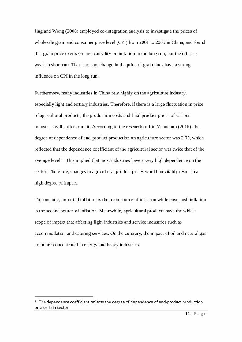
Variance Decomposition –Cholesky Decomposition
Figure 6 Variance Decomposition of LNDEFL_SA
Figure 7 Variance Decomposition of LNM2_SA
Figure 8 Variance Decomposition of LNGDP_SA

40 | P a g e
General speaking, for each independent variable (𝐿𝑁𝐷𝐸𝐹𝐿_𝑆𝐴, 𝐿𝑁𝑀2_𝑆𝐴 and
𝐿𝑁𝐺𝐷𝑃_𝑆𝐴) experiencing a shock, the impact on its own contributes the maximum at
the very beginning, then the impact of it starts to decline. In figure 7 and figure 8, each
curve tends to be horizontal, indicating that the impact of the independent variable
shock on the dependent variables changes gradually and stabilizes finally. Nonetheless,
in figure 6, the impacts on dependent variables other than inflation itself take over the
impact on it. It is not surprising since whenever the government noticed inflation rate is
at a high rate, the PBOC starts to take action to control the inflation. Moreover, the
shock on inflation also affects GDP in the long run.
In figure 6, it shows the impacts on inflation rate, money supply growth and GDP
growth by a shock of inflation rate.17 Firstly, the contribution on inflation rate itself
drops from 100% to 20% within the periods of 1 to 20. Secondly, the contribution on
money supply growth boosts from 0% to 49.6% within the periods of 1 to 15. Thirdly,
the effect of GDP growth upsurges rapidly when comparing with the velocity of money
supply growth, the contribution on it surges 29.8% from 0% in the period of 7. It
implies that change in inflation rate has significant impact on money supply growth and
GDP growth.
In figure 7, it shows the impacts on inflation rate, money supply growth and GDP
growth by a shock of money supply growth.18 Firstly, the contributions on inflation rate
and money supply growth itself fluctuate until middle of the time period. However, they
are moving in opposite direction. The impact on inflation rate rises from 32.3% to
45.3% within the periods of 1 to 3, and then it falls to 28.9% in the period of 7. Besides,
the impact on money supply growth itself declines from 67.7% to 54.5% within the
17 See appendix 1. 18 See appendix 2.

41 | P a g e
periods of 1 to 3, and then it climbs to 65.0% in the period of 7. Secondly, the
contribution on GDP growth increases from 0% to 3.08% within the periods of 1 to 4,
then it further increases into 17% until the period of 20. It shows that change in money
supply growth has significant impact on those three variables, that is inflation rate,
money supply growth as well as GDP growth.
In figure 8, it shows the impacts on inflation rate, money supply growth and GDP
growth by a shock of GDP growth.19 The impacts on inflation rate and GDP growth are
steady after the period of 5, while the impact on money supply growth subsequently
keeps constant in the period of 2. Firstly, the contribution of shock of GDP growth on
inflation accelerates from 0.03% to 17.1% within the periods of 1 to 3, and then it
further increases to 34.5% in the period of 5. Secondly, the contribution on money
supply growth also rises, however remains a short period, from 2.58% to 14.0% within
the periods of 1 to 2. Finally, the contribution on GDP growth itself dives from 97.4%
to 55.0% within the periods of 1 to 5. It represents the change in GDP growth do not
have significant impact on the above three variables.
The above results are basically consistent with the result of Granger causality.
Possible reasons for the results
In the long run relationship, both of the money supply growth and economic growth are
positively related to inflation rate. These results can be explained by QTM and AD-AS
model. QTM stated that velocity of money and real output are fixed in the long run,
therefore, increase in money supply directly causes increase in inflation rate. In AD-AS
19 See appendix 3.
42 | P a g e
model, rise in money supply causes fall in the interest rate, which stimulus the
aggregate demand, it causes rise in price level finally. On the other hand, increase in
GDP also directly shifts the aggregate demand to the right, thus, the price level goes up
and causes inflation.
When it comes to the issue of short run, our empirical study found that money supply
negatively causes inflation rate. It is unlikely to the long run relationship. Since the
inflation rate in this research is represented by the GDP deflator, which largely affected
by the price of imported goods, raw material and agricultural product as I mentioned in
the section (2). Therefore, money supply is not the only source to influence the inflation
rate.
Moreover, the impact of inflation rate on money supply growth fluctuates in the short
run. These findings lead us to believe that there are other variables also affect the
money supply, such as exchange rate. As a manufacturing and export-driven economy
that receives tremendous amounts of foreign exchange (forex) capital for its exports, the
Chinese currency forex rates also impact the country's money supply. China runs a trade
surplus. It sells more to the world than it purchases back.20 Due to the huge supply of
USD and demand for yuan, the rate of yuan can rise against the U.S. dollar. If that
happens, Chinese exports will become costlier and lose their competitive price
advantage in the international market. This will lead to problems for the Chinese
economy, resulting in lesser or no sales of manufactured goods, widespread
unemployment and economic stagnation. The central bank of China PBOC intervenes to
control this situation, and keeps the rates lower through artificial measures.
20 Chinese exporters use USD for their exports, but need to pay for local expenses and wages in
local currency renminbi.

43 | P a g e
Finally, money supply was proved negatively related to economic growth in the short
run. One of the reasons behind is economic growth is more directly influenced by the
growth of the consumption (C), investment (I), government expenditure (G) and net
export (NX). For example, the invertors are pessimistic toward the prospect of
economic environment, the investment drops after all. Since the calculation process of
GDP is directly add up C, I, G and NX. Any changing in the component would directly
affect the GDP itself. Therefore, money supply is not the only factor that affects the
economic growth.
Comparing the results with previous research
Regarding to the long run relationship among money supply, inflation rate and
economic growth, ecm and VECM methods was employed in this paper. Our findings
are in line with Yao (2007) finding21, there was one long run co-integration relationship
among the three variables. Beside, in However, incongruent with Xie, Tang and Cui
(2007) finding22, there was no stable equilibrium among money supply, inflation and
economic growth, and there was no co-integration relationship among the three
variables. Moreover, Liu and Jin (2005) finding23, increase in money supply did not
necessarily lead to inflation. The differences in the finding may possibly attribute to the
difference in estimation method and the data.
21 In his research, he used error correction model and VECM as same as our studies to test the
long run relationship among the three variables within the periods of 1996 to 2006 in China.
22 In their research, they used co- integration approach and testing the ADF salvage. They
employed the data from 1998 to 2007 in China.
23 In their research, VAR model was employed.

44 | P a g e
Another important comparison is the short run Granger causality. Our study has result
that money supply Granger causes inflation which is consistent with Liu (2001), Liu
and Jin (2005) and Yao (2007). They found that money supply stimulates economic
growth in the short run. Ji (2012), however, attained a result that money supply did not
influence inflation rate and economic growth in the short run.24 Accounting for the
differences in the findings, the period of data selected and model selection may help to
explain this issue.
Policy Recommendations
Since the finding told money supply Granger causes inflation rate and economic growth
in short run and they have a positive relationship in the long run. It implies that the
government of China can control the money supply to influence inflation rate and
economic growth. On the one hand, the government of China should implement a
relatively tight monetary policy to suppress the inflation rate at a lower level. On the
other hand, lagged effects of tight monetary policy may lead to economic recession.
Therefore, it is recommended that the PBOC should take measures to reduce the growth
rate of the money supply. By the same time, a cautious regulation should be
implemented for the macroeconomic policy in order to avoid financial risks.
24 In his studies, he covered the monthly data from December of 2006 to December of 2010 to
develop a VAR model.

45 | P a g e
7. Conclusion
In this paper, with the use of Vector Error Correction Model (VECM), error correction
mode (ecm), Johansen co-integration test, Granger causality as well as variance
decomposition, the data of money supply, GDP deflator and real GDP from the period
of first quarter of 1999 to third quarter of 2015 have been employed to test the short run
and long run relationship among money supply growth, inflation rate and GDP growth
in China.
Summary of key findings
From our empirical results, one co-integration equation among the three variables
implies that a long run relationship exists among money supply, inflation rate and
economic growth in China. In short run, a bi-directional causality between money
supply growth and inflation rate was found. Besides, money supply and inflation do
Granger cause economic growth while economic growth does not Granger cause money
supply growth and inflation rate.
Contribution and Recommendations
Undoubtedly, every party involved in national economy must bear in mind the
following objectives: reduce unemployment rate, promoting economic growth and price
stability. Monetary policy is still a major instrument to achieve those goals. Hence,
money supply will still be a critical issue for the government of China to balance the
inflation and economic development simultaneously. To achieve the objectives, a sound

46 | P a g e
monetary policy would be the direction for the PBOC to pursue. A cautious regulation
should be implemented for the macroeconomic policy in order to avoid financial risks.
Limitations of the research
Our model is relatively simple because of time constraint and lack of statistical
significant, this study may not involve all of relevant factors. For instance, other factors
that may have impacts the model are imported price, grain price, agriculture product
price, input price, interest rate and exchange rate.
As mentioned in the above section, using different estimation models and period of data
can generate different conclusion from different research, it is hard to say which
research is more accurate. It is more precise that a better method of estimation would be
found toward the economic aspect.
A reason for further research
There are still a number of potential factors affect this model that are not able to be
included in this paper mainly due to the time constraint. The imported price, grain price,
agriculture product price, input price, interest rate and exchange rate are still waiting to
be experimented. Therefore, it is hoped that all of these potential factors will be well
incorporated in the further research. Hence, estimation will be resulted with more
accurate findings, which will be meaningful for policy decisions.

47 | P a g e
References
Bibliography
Ahmed, A. E. M. & Suliman, S. Z. (2011). The long-run relationship between money
supply, real GDP and price level: Empirical evidence from Sudan. Journal of
Business Studies Quarterly, 2 (2), 68-79.
Bin L. (2001, July). Identification of monetary policy shock and empirical research on
the effectiveness of monetary policy. Journal of Finance, Beijing, 1-9.
Bin L. (2002, July). Empirical research on the relationship among money supply, output
and prices. Journal of Finance, Beijing, 10-16.
Blaug, M. (1995). The quantity theory of money: From Locke to Keynes and Friedman.
Vermont: Edward Elgar.
Boyes, W. J. (1992). Macroeconomics : Intermediate theory and policy. Cincinnati:
South-Western.
McCandles G. & Weber W. (1995, March). Some monetary facts. Federal Reserve
Bank of Minneapolis quarterly review, 2-11.
Darrat, A. F., Shelor, R.M. & Dickens, R. N. (1999). Forecasting corporate performance:
VECM comparison with other time series models. Studies in Economics and
Finance, 19 (2), 49-61.
Engle, R. & Granger, C.W.J. (1987). Cointegration and error correction:
Representation, estimation and testing. Econometrica, 55, 251-76.

48 | P a g e
Gorrie, J. R. (2013). The China crisis: How China's economic collapse will lead to a
global depression. Hoboken: Wiley. doi: 10.1002/9781118705513
Hicks, J. (1980). IS-LM: An explanation. Journal of Post Keynesian Economics, 3 (2),
139-154.
Johansen, S. & Juselius, K. (1990). Maximum likelihood estimation and inference on
cointegration: With application to the demand for money. Oxford Bulletin of
Economics and Statistics, 52, 169-210.
Jing, Y.H. & Wang, X.H. (2006, May). Co-integration analysis on grain average
price and inflation in China from 2001 to 2005. Statistics & Information
Forum.
Lu, J. & Shu, Y. (2002, June). Long-term neutral monetary: Theory and experience in
China”, Journal of Finance, Beijing, 32-40.
Liu, L. & Jin, Y.H. (2005). Money supply, inflation and economic growth in china: the
empirical analysis based on cointegration. Statistical Research, 14-19.
Liu, Y.C. (2015). Managing inflation in China: Current trends and new strategies.
Honolulu: Enrich Professional, 4-25.
Mishra, P. K., Mishra, U. S. & Mishra, S. K. (2010) Money, price and output: A
causality test for India. International Research Journal of Finance and Economics,
53, 26-36
National Bureau of Statistics of China., ed., China Statistical Yearbook, 1999-2015
editions. Beijing: China Statistics Press.

49 | P a g e
Thornton, H. (1802). An enquiry into the nature and effects of the paper credit of Great
Britain. London: Hatchard.
Tobin, J. & Clower, R. W. (1970, May). Is there an optimal money supply. The Journal
of Finance, 25 (2), 425–433. doi: 10.1111/j.1540-6261.1970.tb00665.x
Wang, S.P. (1996, May). The causes of inflation and empirical research on the
relationship among, monetary policy, its economic goals, and macro-control in
China. Quantitative & Technical Economics, Beijing, 17-25.
Wang, S.P. & Li, Z.N. (2004, July). The cointegration analysis of monetary demand and
the monetary policy proposals in China. Economic Research, Beijing, 9-17.
Wong, X. K. & Deng, S. H. (2000, February). On the empirical studies of monetary
policies neutrality and asymmetry. Journal of Management Sciences in China, 6
(2).
Xie, C.H. & Tang, H.F. (2007, December). Economic growth, structural imbalance, and
the excess of liquidity. Journal of Central University of Finance and Economic,
Beijing, 10-16.
Yao, Y. (2007, February). Empirical analysis on the relationship between money
Supply: Inflation and economic growth in China. Economy and Management, 21
(2), 45-47.
辛樹人(2013 年)。〈穩增長與防通脹的動態平衡〉。《中國金融》,第 8 期,
頁 62-63。

50 | P a g e
Website resource
Barboza, D. (2008, November 9). China unveils sweeping plan for economy. The New
York Times. Retrieved April 1, 2016 from, Web site:
http://www.nytimes.com/2008/11/10/world/asia/10china.html?_r=0
Fan, G. & Hope, N.C. (2014). Chapter 16: The role of state-owned enterprises in the
Chinese economy. China U.S. focus, U.S.- China 2022. Retrieved April 1, 2016
from Web site: http://www.chinausfocus.com/2022/index-page_id=1480.html
Graeme, W. (2010, December 3). China to tighten monetary policy to control inflation.
The Guardian. Retrieved April 1, 2016 from Web site:
http://www.theguardian.com/business/2010/dec/03/china-tighten-monetary-policy
-inflation
Trading Economics (2016, March 8). China balance of rrade. Trading Economics
Retrieved April 4, 2016 from Web site:
http://www.tradingeconomics.com/china/balance-of-trade
Toh, H. S. (October 18, 2012). Experts warn on latest China stimulus package. South
China Morning Post. Retrieved April 1, 2016 from, Web site:
http://www.scmp.com/business/global-economy/article/1063516/experts-warn-lat
est-china-stimulus-package

51 | P a g e
Appendix
Appendix 1
Variance Decomposition of LNDEFL_SA
Period S.E. LNDEFL_SA LNM2_SA LNGDP_SA
1 0.005423 100.0000 0.000000 0.000000
2 0.008144 99.10157 0.112249 0.786181
3 0.009494 93.21680 2.242849 4.540348
4 0.010282 79.68323 6.614839 13.70194
5 0.012668 63.05221 11.89663 25.05116
6 0.016464 53.61484 16.57918 29.80598
7 0.020869 47.30118 22.86314 29.83569
8 0.025866 42.06238 29.42114 28.51648
9 0.031339 37.79699 35.38100 26.82201
10 0.036890 34.68274 39.56552 25.75175
11 0.042114 31.90285 42.84361 25.25353
12 0.046908 29.20421 45.50424 25.29155
13 0.051318 26.66889 47.63089 25.70021
14 0.055490 24.54454 48.99054 26.46492
15 0.059476 22.93676 49.58688 27.47636
16 0.063337 21.82518 49.49252 28.68230
17 0.067127 21.11428 48.90629 29.97943
18 0.070923 20.72326 47.99913 31.27762
19 0.074771 20.61563 46.90432 32.48005
20 0.078711 20.76219 45.71221 33.52560

52 | P a g e
Appendix 2
Variance Decomposition of LNM2_SA
Period S.E. LNDEFL_SA LNM2_SA LNGDP_SA
1 0.012046 32.34390 67.65610 0.000000
2 0.019653 42.83658 56.88320 0.280222
3 0.025797 45.26677 54.46380 0.269430
4 0.029487 40.02890 59.35619 0.614917
5 0.033123 32.35313 64.56602 3.080853
6 0.036778 29.65541 65.58088 4.763708
7 0.040364 28.94345 65.04198 6.014576
8 0.042747 29.67150 63.44292 6.885584
9 0.044671 31.40132 60.74431 7.854369
10 0.046336 33.59319 57.86357 8.543237
11 0.047830 35.57802 55.23302 9.188955
12 0.048735 36.43272 53.92862 9.638656
13 0.049279 36.43460 53.42589 10.13951
14 0.049662 36.05961 53.32526 10.61513
15 0.050080 35.52395 53.35531 11.12074
16 0.050631 34.81713 53.56429 11.61858
17 0.051352 33.95007 53.87531 12.17462
18 0.052231 32.97593 54.27135 12.75272
19 0.053215 32.04532 54.58111 13.37357
20 0.054293 31.30843 54.67909 14.01248

53 | P a g e
Appendix 3
Variance Decomposition of LNGDP_SA
Period S.E. LNDEFL_SA LNM2_SA LNGDP_SA
1 0.005047 0.027664 2.582849 97.38949
2 0.007958 3.458215 13.99955 82.54224
3 0.011289 17.08085 13.23412 69.68503
4 0.015151 29.24222 11.49307 59.26471
5 0.020021 34.51183 10.57976 54.90841
6 0.023819 34.28590 10.68731 55.02679
7 0.027603 33.74045 11.53798 54.72157
8 0.031303 33.73464 12.50106 53.76430
9 0.035240 33.98928 12.89983 53.11089
10 0.039077 34.15245 12.68118 53.16637
11 0.042557 33.82769 12.55426 53.61805
12 0.045722 33.35026 12.37389 54.27585
13 0.048859 32.92317 12.16903 54.90780
14 0.052039 32.72931 11.76742 55.50328
15 0.055170 32.72693 11.27986 55.99321
16 0.058221 32.82467 10.75627 56.41906
17 0.061176 32.93102 10.28726 56.78173
18 0.064103 33.07016 9.842922 57.08692
19 0.066987 33.27023 9.437674 57.29210
20 0.069819 33.52740 9.060643 57.41196