ANALYSIS OF WIND-DRIVEN FLOW AND EXTERNAL CONVECTIVE HEAT TRANSFER COEFFICIENTS FOR THE BESTEST MODEL BUILDING

Marcelo Guillaumon Emmel and Nathan Mendes

Thermal Systems Laboratory – LST Pontifical Catholic University of Paraná

Curitiba/PR/Brazil - Zip Code 80215-901 E-mail: marceloemmel@terra.com.br / nathan.mendes@pucpr.br

ABSTRACT

Building energy analysis are very sensitive to external convection heat transfer coefficients so that some researchers have made sensitivity calculations and proved that depending on the choice of convective heat transfer coefficient values, energy demands estimation values can vary from 20 to 40%. In this context, a Computational Fluid Dynamics (CFD) program has been used to predict external convective heat transfer coefficients at external building surfaces. The simulations have been carried out using the building model presented in ANSI/ASHRAE Standard 140-2001 – Standard Method of Test for the Evaluation of Building Energy Analysis Computer Programs in the Building Energy Simulation Test (BESTEST). For the BESTEST house model, effects of wind speed and temperature differences between the surfaces and the external air have been analyzed, showing different heat transfer conditions and coefficients.

Keywords: CFD in Buildings, External Convective Heat Transfer Coefficients.

INTRODUCTION

Building Simulation tools need to better evaluate convective heat exchanges between external air and wall surfaces. Previous analysis demonstrated the significant effects of convective heat transfer coefficient values on the room energy balance. Some authors have pointed out that large discrepancies observed between widely used building thermal models can be attributed to the different correlations used to calculate or impose the value of the convective heat transfer coefficients. Moreover, numerous researchers have made sensitivity calculations and proved that the choice of Convective Heat Transfer Coefficient values can lead to differences from 20% to 40% of energy demands.

Many research works have been conducted since early eighties focused on the convection heat transfer problems inside buildings. To name a few, one should cite Alamdari and Hammond (1983), Awbi (1998), Awbi and Hatton (2000), Beausoleil-Morrison (1999, 2002a, 2002b), Djunaedy et al.

(2004), Fisher (1995), Halcrow (1987), Khalifa and Marshall (1990) and Zhai and Chen (2003).

Nevertheless, not much research has been focused on the determination of external heat transfer coefficients. McAdams (1954) produced a generic empirical correlation using a copper-plate apparatus for forced convection. Grandrille et al. (1983) presented an intermediate-level model to determine convective heat transfer coefficients based also on experiments. In order to provide further information on external convective heat transfer coefficients, a numerical work is presented in this paper, using a Computational Fluid Dynamics (CFD) commercial package (CFX) to predict convective heat transfer coefficients at external building surfaces.

The simulations have been carried out using the model presented in ANSI/ASHRAE Standard 140-2001 – Standard Method of Test for the Evaluation of Building Energy Analysis Computer Programs in the Building Energy Simulation Test (BESTEST), which is a methodology that was employed in 14 programs, participating of International Energy Agency (Judkoff and Neymark, 1995).

Results are presented in terms of sensitivity analysis for outside airflow patterns, grid refinement, wind velocity and temperature difference.

MODELING

Physical Model

For the simulated cases shown in this paper, the BESTEST model (Building Energy Analysis Computer Programs in the Building Energy Simulation Test model) has been used. This physical model is used in a large range of case studies (with simulation and real prototypes) and a wide variety of data is available.

Ninth International IBPSA Conference Montréal, Canada

August 15-18, 2005

- 287 -

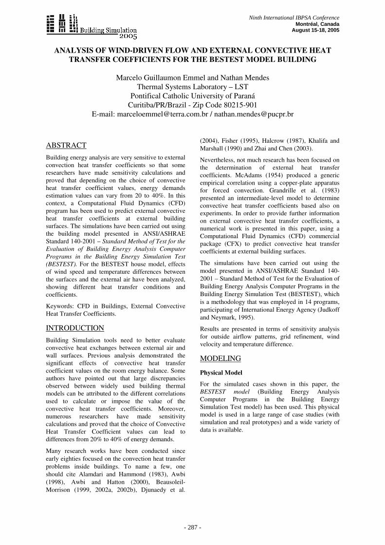
6m

8m

0.5m 0.5m

0.5m

1m

2.7m

2m

3m 3m

0.2m south

Figure 1 The BESTEST model dimensions

Governing Equations The set of transport equations solved by the computational fluid dynamics software are the unsteady Navier-Stokes equations. In principle, the Navier-Stokes equations describe both laminar and turbulent flows without the need for additional information. However, turbulent flows at realistic Reynolds numbers span a large range of turbulent length and time scales and would generally involve length scales much smaller than the smallest finite volume mesh, which can be practically used in a numerical analysis. The Direct Numerical Simulation (DNS) of these flows would require computing power, which is many orders of magnitude higher than available in the foreseeable future. When looking at time scales much larger than the time scales of turbulent fluctuations, turbulent flow could be said to exhibit average characteristics, with an additional time-varying, fluctuating component. Turbulence models based on the Reynolds Averaged Navier-Stokes equations (RANS equations) are known as Statistical Turbulence Models due to the statistical averaging procedure employed to obtain the equations. The used turbulence models seek to solve a modified set of transport equations by introducing averaged and fluctuating components. The instantaneous equations of mass, momentum and energy conservation can be written as follows: The Continuity Equation:

( ) 0=•∇+∂∂

Ut

ρρ (1)

The Momentum Equations:

{ } { } MSuuUUtU +⊗−•∇=⊗•∇+

∂∂ ρτρρ (2)

The Energy Equation:

( ) ( ) ESuUt

+−∇Γ•∇=•∇+∂

∂ φρφφρρφ (3)

where τ is the molecular stress tensor, uu ⊗ρ is the

Reynolds stress and φρu is the Reynolds flux. From the eddy viscosity models:

( )( )Ttt UUUkuu ∇+∇+•∇−−=⊗− µδµδρρ

32

32 (4)

φφρ ∇Γ=− tu (5)

where tµ is the eddy viscosity or turbulent viscosity

and tΓ .is the eddy diffusivity, and can be written as

t

tt Pr

µ=Γ (6)

The above equations can only express the turbulent fluctuation terms of functions of the mean variables if the turbulent viscosity, µ t, is known. The Shear Stress Transport (SST) model has been utilized for the turbulent airflow, due to its good agreement to real cases under similar conditions. This model accounts for the transport of the turbulent shear stress and gives highly accurate predictions of the onset and the amount of flow separation under adverse pressure gradients. The CFD package also allows creating solid regions in which the equations for heat transfer are solved, but with no flow. This is known as Conjugate Heat Transfer, and the solid regions are known as “Solid Domains”. Within Solid Domains, the conservation of energy equation is simplified since there is no flow inside a solid, thus conduction is the only mode of heat transfer. The heat conduction through the solid has the following transport equation:

( ) ( ) Ep STTct

+∇•∇=∂∂ λρ (7)

where ρ, cp and λ are the density, specific heat capacity and thermal conductivity of the solid, respectively.

Problem Setting

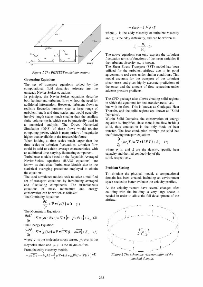
To simulate the physical model, a computational domain has been created, including an environment space needed to better evaluate the velocity profiles.

As the velocity vectors have several changes after colliding with the building, a very large space is needed in order to allow the full development of the airflow.

Figure 2 The schematic representation of the physical domain.

- 288 -

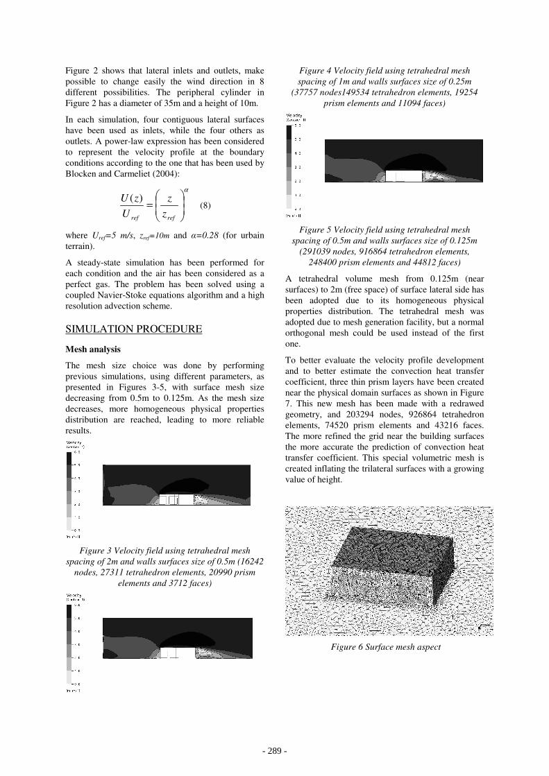
Figure 2 shows that lateral inlets and outlets, make possible to change easily the wind direction in 8 different possibilities. The peripheral cylinder in Figure 2 has a diameter of 35m and a height of 10m.

In each simulation, four contiguous lateral surfaces have been used as inlets, while the four others as outlets. A power-law expression has been considered to represent the velocity profile at the boundary conditions according to the one that has been used by Blocken and Carmeliet (2004):

α

��

�

�

��

�

�=

refref zz

UzU )(

(8)

where Uref=5 m/s, zref=10m and �=0.28 (for urbain terrain).

A steady-state simulation has been performed for each condition and the air has been considered as a perfect gas. The problem has been solved using a coupled Navier-Stoke equations algorithm and a high resolution advection scheme.

SIMULATION PROCEDURE

Mesh analysis

The mesh size choice was done by performing previous simulations, using different parameters, as presented in Figures 3-5, with surface mesh size decreasing from 0.5m to 0.125m. As the mesh size decreases, more homogeneous physical properties distribution are reached, leading to more reliable results.

Figure 3 Velocity field using tetrahedral mesh spacing of 2m and walls surfaces size of 0.5m (16242

nodes, 27311 tetrahedron elements, 20990 prism elements and 3712 faces)

Figure 4 Velocity field using tetrahedral mesh spacing of 1m and walls surfaces size of 0.25m

(37757 nodes149534 tetrahedron elements, 19254 prism elements and 11094 faces)

Figure 5 Velocity field using tetrahedral mesh spacing of 0.5m and walls surfaces size of 0.125m

(291039 nodes, 916864 tetrahedron elements, 248400 prism elements and 44812 faces)

A tetrahedral volume mesh from 0.125m (near surfaces) to 2m (free space) of surface lateral side has been adopted due to its homogeneous physical properties distribution. The tetrahedral mesh was adopted due to mesh generation facility, but a normal orthogonal mesh could be used instead of the first one.

To better evaluate the velocity profile development and to better estimate the convection heat transfer coefficient, three thin prism layers have been created near the physical domain surfaces as shown in Figure 7. This new mesh has been made with a redrawed geometry, and 203294 nodes, 926864 tetrahedron elements, 74520 prism elements and 43216 faces. The more refined the grid near the building surfaces the more accurate the prediction of convection heat transfer coefficient. This special volumetric mesh is created inflating the trilateral surfaces with a growing value of height.

Figure 6 Surface mesh aspect

- 289 -

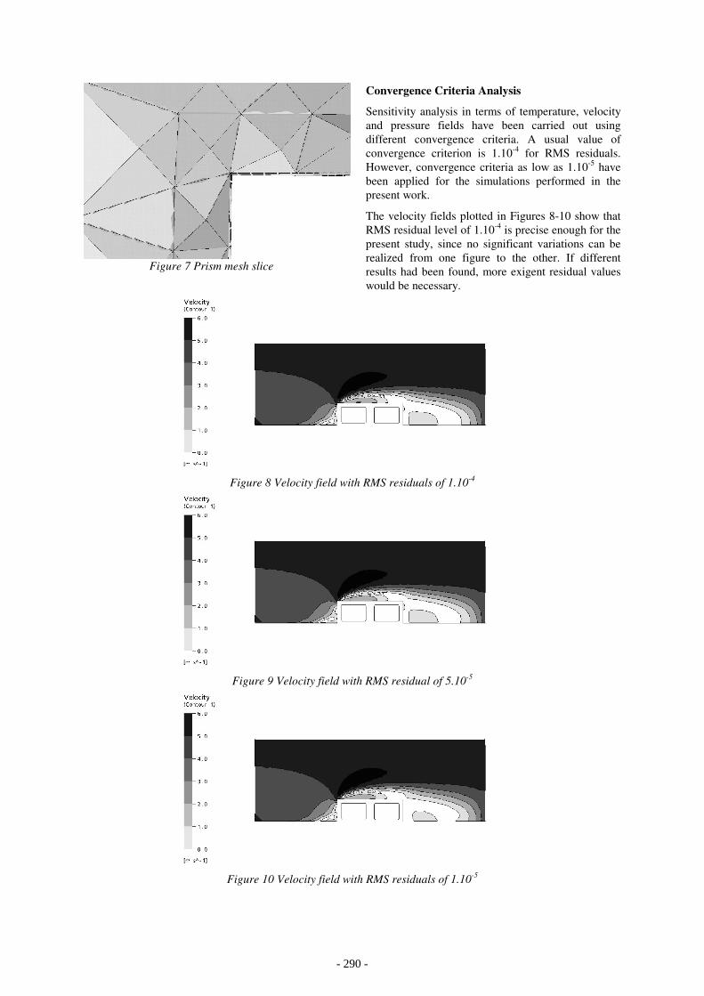
Figure 7 Prism mesh slice

Convergence Criteria Analysis

Sensitivity analysis in terms of temperature, velocity and pressure fields have been carried out using different convergence criteria. A usual value of convergence criterion is 1.10-4 for RMS residuals. However, convergence criteria as low as 1.10-5 have been applied for the simulations performed in the present work.

The velocity fields plotted in Figures 8-10 show that RMS residual level of 1.10-4 is precise enough for the present study, since no significant variations can be realized from one figure to the other. If different results had been found, more exigent residual values would be necessary.

Figure 8 Velocity field with RMS residuals of 1.10-4

Figure 9 Velocity field with RMS residual of 5.10-5

Figure 10 Velocity field with RMS residuals of 1.10-5

- 290 -

Time step Analysis

A constant physical time step has been used throughout the simulations.

For advection dominated flows the physical time step size should be some fraction of a length scale divided by a velocity scale. A good approximation is the Dynamical Time for the flow, given by

UL

t2

=∆ (9)

where L was taken as the roof diagonal size (10m) and U as the air velocity. Therefore, for U=10m/s, 0.5-s physical time step can be considered as a good initial value.

A good time step choice leads to a uniform and consistent convergence history. The right choice will be function of other simplification hypothesis, as the mathematical models and the mesh quality. For this job, 0.5 s revealed to be a good choice.

RESULTS AND DISCUSSIONS

Standard evaluation

In order to better understand the thermal changes and effects on mean convection heat transfer coefficients, some special cases have been analyzed using standard values of wind direction, air velocity and temperature difference.

In the present work only southwest wind direction has been considered, but different values of air velocity (5m/s, 10m/s and 15m/s) and temperature difference (0K, 10K and 20K) have been taken into account for the sensitivity analysis on airflow patterns and on convection heat transfer coefficients at each building surface.

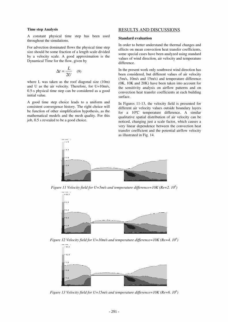
In Figures 11-13, the velocity field is presented for different air velocity values outside boundary layers for a 10ºC temperature difference. A similar qualitative spatial distribution of air velocity can be noticed, changing just a scale factor, which causes a very linear dependence between the convection heat transfer coefficient and the potential airflow velocity as illustrated in Fig. 14.

Figure 11 Velocity field for U=5m/s and temperature difference=10K (Re=2. 106)

Figure 12 Velocity field for U=10m/s and temperature difference=10K (Re=4. 106)

Figure 13 Velocity field for U=15m/s and temperature difference=10K (Re=6. 106)

- 291 -

External Convective Heat Transfer Coefficients

-

10,00 20,00 30,00 40,00 50,00 60,00 70,00

ROOF W WEST W NORTH W SOUTH W EAST

h [W

/m².K

]

SE Wind, V=5 m/s, DeltaT=10 SE Wind, V=10 m/s, DeltaT=10 SE Wind, V=15 m/s, DeltaT=10

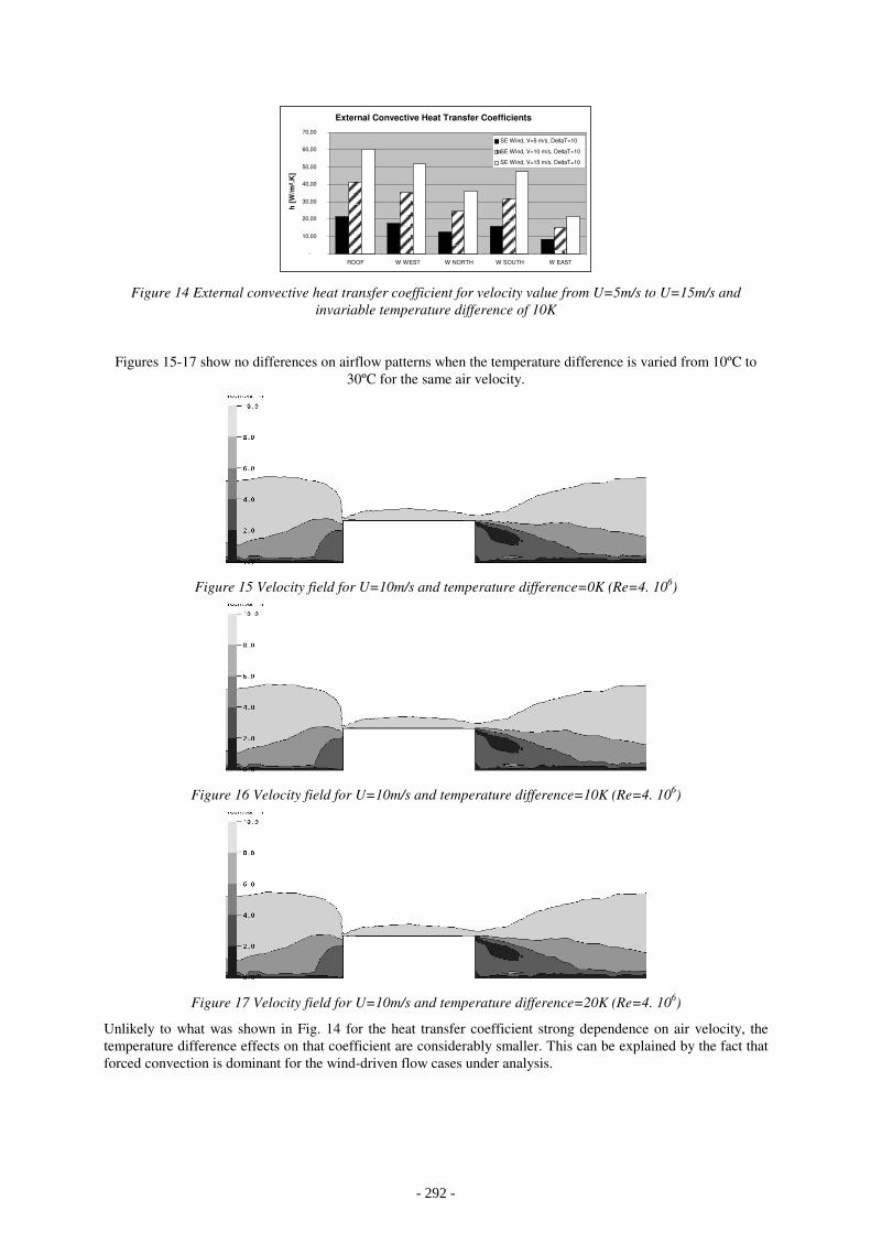
Figure 14 External convective heat transfer coefficient for velocity value from U=5m/s to U=15m/s and invariable temperature difference of 10K

Figures 15-17 show no differences on airflow patterns when the temperature difference is varied from 10ºC to 30ºC for the same air velocity.

Figure 15 Velocity field for U=10m/s and temperature difference=0K (Re=4. 106)

Figure 16 Velocity field for U=10m/s and temperature difference=10K (Re=4. 106)

Figure 17 Velocity field for U=10m/s and temperature difference=20K (Re=4. 106)

Unlikely to what was shown in Fig. 14 for the heat transfer coefficient strong dependence on air velocity, the temperature difference effects on that coefficient are considerably smaller. This can be explained by the fact that forced convection is dominant for the wind-driven flow cases under analysis.

- 292 -

External Convective Heat Transfer Coefficients

-

5,00 10,00 15,00 20,00 25,00 30,00 35,00 40,00 45,00

ROOF W WEST W NORTH W SOUTH W EAST

h [W

/m².K

] SE Wind, V=10 m/s, DeltaT=0 SE Wind, V=10 m/s, DeltaT=10 SE Wind, V=10 m/s, DeltaT=20

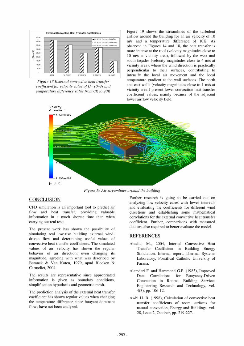
Figure 18 External convective heat transfer coefficient for velocity value of U=10m/s and temperature difference value from 0K to 20K

Figure 19 shows the streamlines of the turbulent airflow around the building for an air velocity of 10 m/s and a temperature difference of 10K. As observed in Figures 14 and 18, the heat transfer is more intense at the roof (velocity magnitudes close to 10 m/s at vicinity area), followed by the west and south façades (velocity magnitudes close to 4 m/s at vicinity area), where the wind direction is practically perpendicular to their surfaces, contributing to intensify the local air movement and the local temperature gradient at the wall surfaces. The north and east walls (velocity magnitudes close to 1 m/s at vicinity area ) present lower convection heat transfer coefficient values, mainly because of the adjacent lower airflow velocity field.

Figure 19 Air streamlines around the building

CONCLUSION

CFD simulation is an important tool to predict air flow and heat transfer, providing valuable information in a much shorter time than when carrying out real tests.

The present work has shown the possibility of simulating real low-rise building external wind-driven flow and determining useful values of convective heat transfer coefficients. The simulated values of air velocity has shown the regular behavior of air direction, even changing its magnitude, agreeing with what was described by Beranek & Van Koten, 1979, apud Blocken & Carmeliet, 2004.

The results are representative since appropriated information is given as boundary conditions, simplification hypothesis and geometric mesh.

The prediction analysis of the external heat transfer coefficient has shown regular values when changing the temperature difference since buoyant dominant flows have not been analyzed.

Further research is going to be carried out on analyzing low-velocity cases with lower intervals and evaluating the coefficients for different wind directions and establishing some mathematical correlations for the external convective heat transfer coefficient. Further, comparisons with measured data are also required to better evaluate the model.

REFERENCES

Abadie, M., 2004, Internal Convective Heat Transfer Coefficient in Building Energy Simulation. Internal report, Thermal Systems Laboratory, Pontifical Catholic University of Parana.

Alamdari F. and Hammond G.P. (1983), Improved Data Correlations for Buoyancy-Driven Convection in Rooms, Building Services Engineering Research and Technology, vol. 4(3), pp. 106-12.

Awbi H. B. (1998), Calculation of convective heat transfer coefficients of room surfaces for natural convection, Energy and Buildings, vol. 28, Issue 2, October, pp. 219-227.

- 293 -

Awbi H. B. and Hatton A. (2000), Mixed convection from heated room surfaces, Energy and Buildings, vol. 32, Issue 2, July, pp. 153-166.

Baker, A, Wong, K. L., Winowich, N.S., Design and Assessment of a Very Large-Scale CFD Industrial Ventilation Flowfield Simulation, AC-02-17-2, pp. 1-6

Beausoleil-Morrison I (2002b)., The adaptive conflation of computational fluid dynamics with whole-building thermal simulation, Energy and Buildings, vol. 34, Issue 9, October, pp. 857-871.

Beausoleil-Morrison I. (1999), Modeling mixed convection heat transfer at internal building surfaces, Proc. Building Simulation’99, vol. 1, pp. 313-320.

Beausoleil-Morrison I. (2002a), The adaptive simulation of convective heat transfer at internal building surfaces, Building and Environment, vol. 37, Issues 8-9, August-September, pp. 791-806.

Beranek, W.J., Koten, H. 1979, Beperken van windhinder om gebouwen, deel 1, Stichting Bouwresearch no. 65, Kluwer Technische Boeken BV, Deventer

Blocken, B., Carmeliet, J. 2004. A review of wind-driven rain research in building science, Journal of Wind Engineering and Industrial Aerodynamics No. 92, pp. 1079-1130

Blocken, B., Carmeliet, J. 2004. Pedestrian Wind Enviroment around Buildings: Literature Review and Parctical Examples, Journal of Thermal Env. & Bldg. Sci., Vol 28, No. 2, 04, Oct, pp. 107-159

Blocken, B., Roels, S., Carmeliet, J. 2004. Modification of pedestrian wind comfort in the Silvertop Tower passages by an automatic control system, Journal of Wind Engineering and Industrial Aerodynamics No. 92, pp. 849-873

CFX 5.7 Help files

Davenport, A.G. 1960. Rationale for Determining Design Wind Velocities, Journal of the Structural Division, Proceedings American Society Civil Engineers, 86, May, pp. 39-68.

Davenport, A.G. 1961. The Application of Statistical Concepts to the Wind Loading of Structure, In: Proceedings Institution of Civil Engineers, Aug

Djunaedy E., Hensen J.L.M. and Loomans M.G.L.C. (2004), Comparing internal and

external run-time coupling of CFD and building energy simulation software, Proc. 9th Int. Conf. on Air Distribution in Rooms - ROOMVENT 2004, 5 - 8 September, University of Coimbra, Coimbra.

Fisher D.E. (1995), An Experimental Investigation of Mixed Convection Heat Transfer in a Rectangular Enclosure, PhD Thesis, University of Illinois, Urbana USA.

Grandrille, T.; Hammond, G. P.; Melo,C.. An Iintermediate-level model of external convection for building energy simulation. Energy And Buildings, USA, v. 12, n. 1, p. 53-66, 1988.

Halcrow (1987), Report on heat transfer at internal building surfaces, Department of Energy, ref: ETSU S1193-P1.

Judkoff R. and Neymark J. (1995), International Energy Agency Building Energy Simulation Test (BESTEST) and Diagnosis Method, NREL/TP - 471-6231. Golden, CO National Renewable Energy Laboratory.

Khalifa A. J. N. (2001b), Natural convective heat transfer coefficient – a review: II. Surfaces in two-and three-dimensional enclosures, Energy Conversion and Management, vol. 42, Issue 4, March, pp. 505-517.

Khalifa A. J. N. (2001a), Natural convective heat transfer coefficient – a review: I. Isolated vertical and horizontal surfaces, Energy Conversion and Management, vol. 42, Issue 4, March, pp. 491-504.

Khalifa A.J.N. and Marshall R.H. (1990), Validation of Heat Transfer Coefficients on Interior Building Surfaces Using a Real-Sized Indoor Test Cell, Int. J. Heat and Mass Transfer, vol. 33 (10), pp. 2219-2236.

MacAdams W. H., 1954, Heat Transmission, New York, McHraw-Hill.

Miles, S, Westbury, P, Practical Tools for Wind Engineering in the Built Environment, QNET-CFD Network Newsletter, Volume 2, No. 2 – July 2003, pp 11-14

Zhai Z. and Chen Q. (2003), Numerical determination and treatment of convective heat transfer coefficient in the coupled building energy and CFD simulation, Building and Environment, vol. 39, 2004, pp. 1001-1009.

Zhai Z. and Chen Q. (2003), Solution characters of iterative coupling between energy simulation and CFD programs, Energy and Buildings, vol. 35, Issue 5, June, pp. 493-505.

- 294 -