Analysis of Very Fast Transients Using Black Box

energies

Article

Analysis of Very Fast Transients Using Black BoxMacromodels in ATP-EMTP

Jonathan James 1,*, Maurizio Albano 1 , David Clark 1, Dongsheng Guo 2 andAbderrahmane (Manu) Haddad 1

1 Advanced High Voltage Engineering and Research Centre, Cardiff University, Cardiff CF24 3AA, UK;[email protected] (M.A.); [email protected] (D.C.); [email protected] (A.H.)

2 National Grid, National Grid House, Warwick Technology Park, Gallows Hill, Warwick CV34 6DA, UK;[email protected]

* Correspondence: [email protected]

Received: 20 December 2019; Accepted: 3 February 2020; Published: 6 February 2020

Abstract: Modelling for very fast transients (VFTs) requires good knowledge of the behaviour ofgas insulated substation (GIS) components when subjected to high frequencies. Modelling usuallytakes the form of circuit-based insulation coordination type studies, in an effort to determine themaximum overvoltages and waveshapes present around the system. At very high frequencies,standard transmission line modelling assumptions may not be valid. Therefore, the approach tomodelling of these transients must be re-evaluated. In this work, the high frequency finite elementanalysis (FEA) was used to enhance circuit-based models, allowing direct computation of parametersfrom geometric and material characteristics. Equivalent models that replicate a finite element model’sfrequency response for bus-spacer and 90 elbow components were incorporated in alternativetransients program-electromagnetic transients program (ATP-EMTP) using a pole-residue equivalentcircuit derived following rational fitting using the well-established and robust method of vectorfitting (VF). A large model order is often required to represent this frequency dependent behaviourthrough admittance matrices, leading to increased computational burden. Moreover, while highlyaccurate models can be derived, the data extracted from finite element solutions can be non-passive,leading to instability when included in time domain simulations. A simple method of improvedstability for FEA derived responses along with a method for identification of a minimum requiredmodel order for stability of transient simulations is proposed.

Keywords: gas insulated substations (GIS); very fast transients (VFT); finite element analysis(FEA), finite element method (FEM); electromagnetic transients program (EMTP); vector fitting(VF); macromodelling

1. Introduction

With the exception of certain types of electromagnetic pulse (EMP) phenomena, very fasttransients (VFTs) are the highest frequency class of transients that pose a direct threat to the insulationof high voltage equipment. They are damped oscillatory transients most commonly associated withdisconnector switching in gas insulated substations (GIS). During disconnector operation, due toits relatively slow movement, multiple breakdowns of the gas gap will occur between the contacts.During each breakdown event, following the subsequent collapse of the electric field sustainedbetween the contacts, an EMP is initiated with a rise time of several nanoseconds and propagatesthroughout the system, reflecting, refracting and attenuating at discontinuities. The superpositionof electromagnetic waves at any point within the system can lead to overvoltages, termed very fasttransient overvoltages (VFTOs), which have magnitudes up to 2.5 pu, with frequencies extending up to

Energies 2020, 13, 698; doi:10.3390/en13030698 www.mdpi.com/journal/energies

http://www.mdpi.com/journal/energies

http://www.mdpi.com

https://orcid.org/0000-0002-5486-4299

https://orcid.org/0000-0003-4153-6146

http://dx.doi.org/10.3390/en13030698

http://www.mdpi.com/journal/energies

https://www.mdpi.com/1996-1073/13/3/698?type=check_update&version=2

Energies 2020, 13, 698 2 of 17

100 MHz [1]. VFTs have been identified as a potential threat to insulation through ageing and surfacebreakdown and are also a significant source of interference to control systems through both conducted,near field and far field coupling [2].

Accurate modelling and simulation of a GIS is essential for equipment design,insulation coordination and even for post-failure investigations following surface flashover ofinsulating spacers. One of the principal outcomes for VFT studies is the correct estimation of reflectedand transmitted electromagnetic wave behaviour at impedance discontinuities. Determination of acomponent’s transient behaviour is essential for the accurate calculation of the maximum overvoltage,waveshape and frequency content; all important factors when trying to determine the probabilityof a breakdown under VFTO. Following a modelling task, it should be possible to identify thepotential system vulnerabilities, allowing informed, preventative action to be taken to avoid furtherrisk. A circuit-based modelling approach for VFTs consists of an electromagnetic transient (EMT)study, which involves the representation of each component within the range of interest by itslumped or distributed parameters. Models are constructed to incorporate each anticipated change incharacteristic impedance.

While models for VFT analysis are very detailed, interaction with the wider system is notusually a concern, owing to the perceived increase in attenuation of high frequency electromagneticwaves when propagating externally over a lossy ground. Distributed line models should accountfor frequency-dependent behaviour, which is evident across the VFT frequency range. However,existing frequency-dependent line models available in alternative transients program-electromagnetictransients program (ATP-EMTP) [3] have proven to be numerically unstable at very high frequencies [4].New methods reported in [5], adopt a modified transmission line approximation, due to the possiblemode conversion for waves propagating over a lossy ground from transverse electromagnetic (TEM)mode to surface wave propagation in the VFT frequency range, which are subject to lower attenuation.This finding could impact the extent of the region under study and also allow numerically stable,frequency-dependent line or cable parameters to be produced directly in ATP-EMTP.

In this paper, an alternative method to the parameter-based calculation approach, commonly usedby various EMTPs is proposed. The method is adapted from those used in simulations for highfrequency printed circuit board (PCB) development, utilising elements of circuit-based modelling,along with enhancements, introduced through finite element analysis (FEA), which is the applicationof the finite element method (FEM). Through the combined use of circuit-based and FEA methods,a more accurate estimation of component behaviour can be realised. The proposed method focusseson the extraction of frequency dependent behaviour from finite element models, initially in the formof scattering parameters (S-parameters) which describe a component’s reflection and transmissioncoefficients. Following the conversion of S-parameters to admittance matrices, the frequency-dependentbehaviour is captured as a rational function approximation using vector fitting (VF). This rationalapproximation is then used to derive multiple order, pole-residue equivalent circuits, capable ofreplicating a component’s frequency response. With any VF derived model, a major concern is thestability of the model in the time domain. To achieve stability, the model must be passive, i.e., it mustnot generate energy. Passivity enforced, high order models produce good results in most cases,although the incorporation of many high order models in a large circuit can exceed program limits.As a result, a systematic approach was developed to identify the lowest possible order approximationfor a stable transient simulation, prior to its inclusion in ATP-EMTP, giving significant savings in bothuser and computation times.

The proposed techniques can be applied to most passive GIS components. However, for thepurpose of this study, the techniques were compared with a circuit-based modelling approach fortwo complex and important GIS components, the bus-spacer and the 90 elbow. The bus-spacerand 90 elbow equivalent models were included in ATP-EMTP, replacing their traditional lumpedand distributed component representations. Simulations were then carried out for several circuittermination scenarios in order to determine any limitations of the proposed method. As with any

Energies 2020, 13, 698 3 of 17

modelling technique, model validation is of the highest importance and is usually achieved byperforming controlled on-site or laboratory-based measurements. In the absence of measurement data,validation was achieved by comparison with results produced using the proven software package,advanced design system (ADS) [6]. ADS permits the inclusion of multiple components via theirS-parameters directly in transient simulations, using a convolution-based technique. This allows singleor multiple pole-residue equivalents to be validated.

2. Finite Element Method for Very Fast Transients

While computationally intensive, FEA can provide a more intuitive understanding of the complexbehaviour of various components and materials when subjected to a set of physical conditions.Finite element modelling for electromagnetic applications can be divided into static, low and highfrequencies. Static and low frequency simulations can be useful for obtaining a good initial estimate forconditions at the lower end of the VFT spectrum. However, the accuracy of solutions deteriorates asthe wavelength approaches the geometric dimensions of the system under study. As a rule of thumb,for frequencies above which the dimensions of a component exceed one tenth of the correspondingwavelength, a full-wave solution is required [7]. In the VFT frequency range, the coaxial bus canbehave as a coaxial waveguide, with many changes in characteristic impedance (discontinuities) andnumerous unshielded apertures from which fields can couple externally or radiate. It is, therefore,more appropriate to analyse the problem in terms of electromagnetic waves.

At very high frequencies, when observing distributed components, voltages and currents arenot easily determined, as their distribution within a system varies spatially and temporally. At aspecific location, these quantities are considered as the line integrals of electric and magnetic fieldsrespectively [8], as given by Equations (1) and (2).

V = −

∫E·dl (1)

I =∮

H·dl (2)

where E and H are the electric and magnetic field vectors, respectively.Instead, at very high frequencies, it is more appropriate to represent components by

their S-parameters, which are multi-port representations of complex reflection and transmissioncoefficients [8], as shown in Equation (3).[

b1

b2

]=

[S11 S12

S21 S22

][a1

a2

](3)

where a1 and a2 are related to reflected voltage waves, b1 and b2 are related to transmitted voltagewaves of their respective ports.

S-parameters are commonly used to characterise the frequency-dependent behaviour of devices inmany high frequency engineering disciplines, as they simply and effectively describe the relationshipbetween incident and reflected waves at the device ports when terminated with a chosen referenceimpedance. While they are also useful for the characterisation of components at low frequencies, they areparticularly useful for identifying the behaviour of components when subjected to high-frequencyconditions, where parasitic capacitances and inductances become more relevant but are sometimesdifficult to predict or incorporate in circuit-based models. Some circuit simulators allow S-parametersto be included directly in transient and frequency domain simulations. For simulators without thisfunctionality, the information contained can be converted to alternative forms including impedanceand admittance parameters [9].

Energies 2020, 13, 698 4 of 17

While the physics of a finite element simulation are dependent on the type of study beingperformed, for a general frequency domain VFT study using FEA [10], a weak form of a boundaryvalue problem representing a time harmonic wave equation of the form given in Equation (4) is solved.

∇× µr−1

(∇× E

)− k0

2(εr −

(jσωε0

))E = 0 (4)

where εr is the relative permittivity, µr is the relative permeability, k0 is the wavenumber of free space,σ is the electrical conductivity, and E is the electric field vector.

For completely enclosed sections of bus, the skin effect confines the transients internally for theVFT frequency range and above. Meshing of the entire metallic domain can thus be avoided and metallosses can be accounted for by applying an impedance boundary condition, represented by Equation(5). √

µr

εr − jσ/ωn×H + E−

(n·E

)n =

(n·Es

)n− Es (5)

where H is the magnetic field vector, n is the unit vector, i.e., a vector perpendicular to the boundarysurface with a magnitude of 1, and Es is the source electric field vector used to specify a source surfacecurrent on the boundary [10].

For a completely sealed system, only the gaseous domain within the bus and dielectric barriersrequire meshing for computations. Where apertures are present, such as the gas-air bushing orunshielded spacer, an external air domain may be required. A Scattering boundary condition, given inEquation (6) can be applied to the outer walls of the external air domain to absorb outgoing waves,reducing unrealistic reflections from the discontinuity created by an artificially truncated domain.For any other conductive boundary, where losses are of no concern, the perfect electric conductor(PEC) boundary condition of Equation (7) is applied.

n×(∇× E

)− jkn×

(E× n

)−

12 jk0∇×

(nn·

(∇× E

))= 0 (6)

n× E = 0 (7)

A port boundary condition can provide both excitation of the structure and absorption of outgoingwaves. Complex port shapes require numerical analysis to determine the propagation modes ata specific frequency. Simple port shapes, such as the coaxial port, allow specification of the portimpedance, calculated analytically for a coaxial structure, as shown in Equation (8). Lumped portsprovide a convenient method of excitation and absorption at the frequencies of interest, while alsoallowing the extraction of S-parameters and hence, provide sufficient detail to enable the extraction offrequency dependent behaviour for the enhancement of circuit models.

Zc =60√εr

ln(

Rout

Rin

)(8)

where εr is the dielectric constant, Rout is the radius of the enclosure, and Rin is the radius of themain conductor.

To demonstrate the use of FEA for GIS components, the bus-spacer intersection and 90 elbowmodels, shown in Figure 1, were created using the RF module of COMSOL Multiphysics® (Burlington,MA, USA) [10]. Insulating spacers provide mechanical support to the HV conductor and can provide agas tight partition between gas zones.

Electric and magnetic field distributions become extremely complex at the bus–spacer junction,particularly at high frequencies. They are a common location for surface discharges under VFTs; hence,the importance of accurate circuit representations is crucial. The 90 elbow is another complex GIScomponent. At very high frequencies, the 90 angle can encourage resonances and even the conversion

Energies 2020, 13, 698 5 of 17

to higher order transverse electric (TE) or transverse magnetic (TM) modes of propagation [11].For many GIS components, even in the VFT frequency range, standard transmission line assumptionsmay no longer be valid [12].

Energies 2020, 13, x 4 of 16

For completely enclosed sections of bus, the skin effect confines the transients internally for the VFT frequency range and above. Meshing of the entire metallic domain can thus be avoided and metal losses can be accounted for by applying an impedance boundary condition, represented by Equation (5). 𝜇𝜀 − 𝑗𝜎/𝜔 𝑛 × 𝐻 + 𝐸 − (𝑛 ∙ 𝐸)𝑛 = (𝑛 ∙ 𝐸 )𝑛 − 𝐸 (5)

where 𝐻 is the magnetic field vector, 𝑛 is the unit vector, i.e., a vector perpendicular to the boundary surface with a magnitude of 1, and 𝐸 is the source electric field vector used to specify a source surface current on the boundary [10].

For a completely sealed system, only the gaseous domain within the bus and dielectric barriers require meshing for computations. Where apertures are present, such as the gas-air bushing or unshielded spacer, an external air domain may be required. A Scattering boundary condition, given in Equation (6) can be applied to the outer walls of the external air domain to absorb outgoing waves, reducing unrealistic reflections from the discontinuity created by an artificially truncated domain. For any other conductive boundary, where losses are of no concern, the perfect electric conductor (PEC) boundary condition of Equation (7) is applied. 𝑛 × (∇ × 𝐸) − 𝑗𝑘𝑛 × (𝐸 × 𝑛) − 12𝑗𝑘 ∇ × 𝑛𝑛 ∙ (∇ × 𝐸) = 0 (6) 𝑛 × 𝐸 = 0 (7)

A port boundary condition can provide both excitation of the structure and absorption of outgoing waves. Complex port shapes require numerical analysis to determine the propagation modes at a specific frequency. Simple port shapes, such as the coaxial port, allow specification of the port impedance, calculated analytically for a coaxial structure, as shown in Equation (8). Lumped ports provide a convenient method of excitation and absorption at the frequencies of interest, while also allowing the extraction of S-parameters and hence, provide sufficient detail to enable the extraction of frequency dependent behaviour for the enhancement of circuit models. 𝑍 = 60√𝜀 𝑙𝑛 𝑅𝑅 (8)

where εr is the dielectric constant, Rout is the radius of the enclosure, and Rin is the radius of the main conductor.

To demonstrate the use of FEA for GIS components, the bus-spacer intersection and 90° elbow models, shown in Figure 1, were created using the RF module of COMSOL Multiphysics® (Burlington, MA, USA) [10]. Insulating spacers provide mechanical support to the HV conductor and can provide a gas tight partition between gas zones.

(a) (b)

Figure 1. Three dimensional finite element models: (a) section of bus-spacer intersection; and (b) 90° elbow. Figure 1. Three dimensional finite element models: (a) section of bus-spacer intersection; and (b)90 elbow.

The spacers are represented by a conical geometry with the material defined by some basicelectrical properties for epoxy resin; permittivity, permeability and conductivity. Dielectric andresistive losses are included using a complex permittivity and a finite conductivity. To simplify themodels for the purpose of this study, the external surfaces of the spacers (radiating apertures) wereassigned PEC boundaries, providing a significant saving in computation time (up to 62% for the entirefrequency sweep). A summary of the simulation parameters is provided in Table 1. The results inS-parameter format (reflectance and transmittance) are given in Figure 2.

Table 1. Summary of finite element method (FEM) simulation parameters.

Parameter Bus-Spacer 90 Elbow

Materials

Aluminium 1

Steel 1

Epoxy Resin: εr = 4.1, µr= 1,σ = 1 × 10−17 (S), tan δ = 2 × 10−7

SF6: εr= 1.002, µr= 1, σ = 0

Aluminium 1

Steel 1

Epoxy Resin: εr = 4.1, µr= 1,σ = 1 × 10−17 (S), tan δ = 2 × 10−7

SF6: εr= 1.002, µr= 1, σ = 0

Mesh Tetrahedral-177,116 elements Tetrahedral-241,846 elements

Computation time 3 h 19 min 2 4 h 28 min 2

1 Material selection not meshed; Impedance Boundary Condition applied. Standard COMSOL Multiphysics®

library materials used [10]; 2 Computation time using 2 x Intel(R) Xeon(R) CPU E5-2670 0 at 2.60 GHz, 16 cores eachand 128 GB RAM. Frequency sweep 0.2–150 MHz.

Energies 2020, 13, x 5 of 16

Electric and magnetic field distributions become extremely complex at the bus–spacer junction, particularly at high frequencies. They are a common location for surface discharges under VFTs; hence, the importance of accurate circuit representations is crucial. The 90° elbow is another complex GIS component. At very high frequencies, the 90° angle can encourage resonances and even the conversion to higher order transverse electric (TE) or transverse magnetic (TM) modes of propagation [11]. For many GIS components, even in the VFT frequency range, standard transmission line assumptions may no longer be valid [12].

The spacers are represented by a conical geometry with the material defined by some basic electrical properties for epoxy resin; permittivity, permeability and conductivity. Dielectric and resistive losses are included using a complex permittivity and a finite conductivity. To simplify the models for the purpose of this study, the external surfaces of the spacers (radiating apertures) were assigned PEC boundaries, providing a significant saving in computation time (up to 62% for the entire frequency sweep). A summary of the simulation parameters is provided in Table 1. The results in S-parameter format (reflectance and transmittance) are given in Figure 2.

Table 1. Summary of finite element method (FEM) simulation parameters.

Parameter Bus-Spacer 90° Elbow

Materials

Aluminium 1

Steel 1 Epoxy Resin: εr = 4.1, μr = 1, σ = 1 × 10−17 (S), tan δ = 2 × 10−7

SF6: εr = 1.002, μr = 1, σ = 0

Aluminium 1

Steel 1 Epoxy Resin: εr = 4.1, μr = 1, σ = 1 × 10−17 (S), tan δ = 2 × 10−7

SF6: εr = 1.002, μr = 1, σ = 0 Mesh Tetrahedral-177,116 elements Tetrahedral-241,846 elements

Computation time 3 h 19 min 2 4 h 28 min 2 1 Material selection not meshed; Impedance Boundary Condition applied. Standard COMSOL Multiphysics® library materials used [10]; 2 Computation time using 2 x Intel(R) Xeon(R) CPU E5-2670 0 at 2.60 GHz, 16 cores each and 128 GB RAM. Frequency sweep 0.2–150 MHz.

(a) (b)

Figure 2. Bus-spacer and elbow scattering parameters (S-parameters): (a) S11 (reflectance); and (b) S21 (transmittance).

3. Vector Fitting and Equivalent Circuit Extraction

As discussed in the previous section, many elements of the GIS are represented as distributed parameter lines. Where multiple frequencies are anticipated, it is common practice to initialise line models at a dominant frequency. With the wide spectrum present in VFTs, this can result in the inaccurate treatment of other frequencies. While frequency-dependent distributed parameter line models exist in ATP-EMTP, the Carson/Pollaczek earth return approaches, on which many line models are based, do not accurately account for displacement currents in regions with εr > 1 at very high frequencies [13]. These earth return admittances are, however, inherently considered when using field solvers that implement full Maxwell’s equations, when appropriate modelling domains are included. Several commercial software packages allow full frequency-dependent models through the use of black box macromodels, created with rational approximations of a frequency response

Figure 2. Bus-spacer and elbow scattering parameters (S-parameters): (a) S11 (reflectance); and (b)S21 (transmittance).

Energies 2020, 13, 698 6 of 17

3. Vector Fitting and Equivalent Circuit Extraction

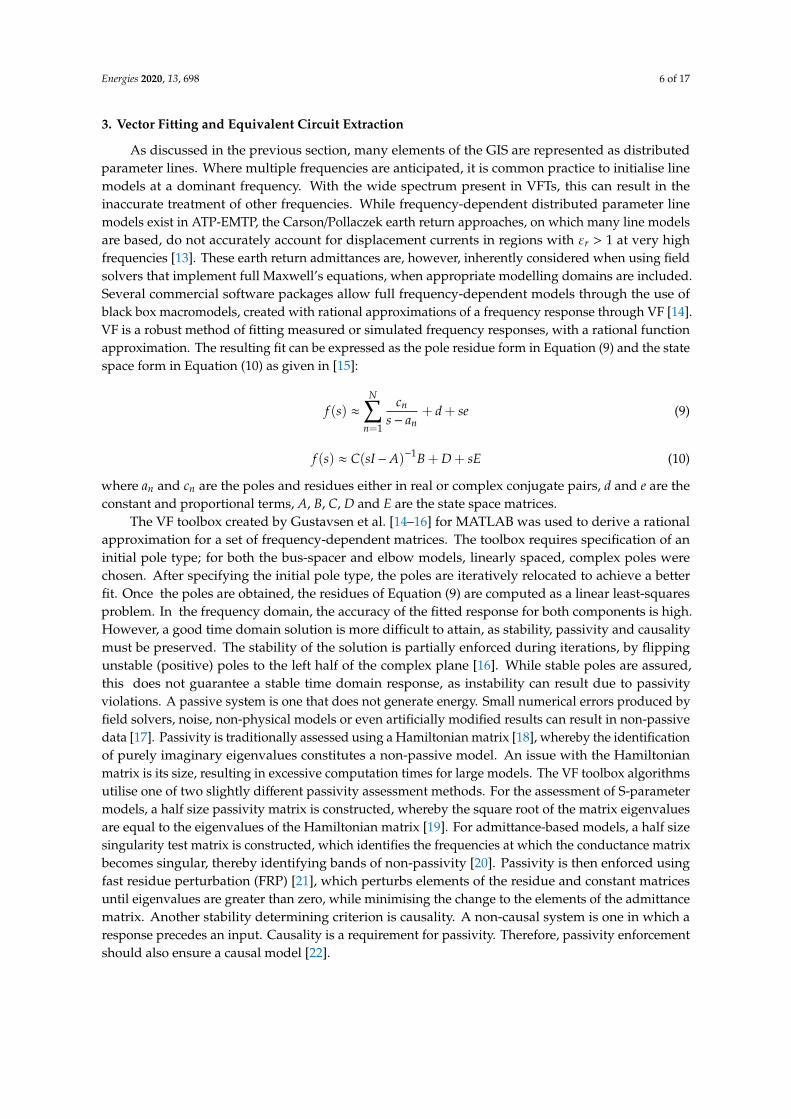
As discussed in the previous section, many elements of the GIS are represented as distributedparameter lines. Where multiple frequencies are anticipated, it is common practice to initialise linemodels at a dominant frequency. With the wide spectrum present in VFTs, this can result in theinaccurate treatment of other frequencies. While frequency-dependent distributed parameter linemodels exist in ATP-EMTP, the Carson/Pollaczek earth return approaches, on which many line modelsare based, do not accurately account for displacement currents in regions with εr > 1 at very highfrequencies [13]. These earth return admittances are, however, inherently considered when using fieldsolvers that implement full Maxwell’s equations, when appropriate modelling domains are included.Several commercial software packages allow full frequency-dependent models through the use ofblack box macromodels, created with rational approximations of a frequency response through VF [14].VF is a robust method of fitting measured or simulated frequency responses, with a rational functionapproximation. The resulting fit can be expressed as the pole residue form in Equation (9) and the statespace form in Equation (10) as given in [15]:

f (s) ≈N∑

n=1

cn

s− an+ d + se (9)

f (s) ≈ C(sI −A)−1B + D + sE (10)

where an and cn are the poles and residues either in real or complex conjugate pairs, d and e are theconstant and proportional terms, A, B, C, D and E are the state space matrices.

The VF toolbox created by Gustavsen et al. [14–16] for MATLAB was used to derive a rationalapproximation for a set of frequency-dependent matrices. The toolbox requires specification of aninitial pole type; for both the bus-spacer and elbow models, linearly spaced, complex poles werechosen. After specifying the initial pole type, the poles are iteratively relocated to achieve a betterfit. Once the poles are obtained, the residues of Equation (9) are computed as a linear least-squaresproblem. In the frequency domain, the accuracy of the fitted response for both components is high.However, a good time domain solution is more difficult to attain, as stability, passivity and causalitymust be preserved. The stability of the solution is partially enforced during iterations, by flippingunstable (positive) poles to the left half of the complex plane [16]. While stable poles are assured,this does not guarantee a stable time domain response, as instability can result due to passivityviolations. A passive system is one that does not generate energy. Small numerical errors produced byfield solvers, noise, non-physical models or even artificially modified results can result in non-passivedata [17]. Passivity is traditionally assessed using a Hamiltonian matrix [18], whereby the identificationof purely imaginary eigenvalues constitutes a non-passive model. An issue with the Hamiltonianmatrix is its size, resulting in excessive computation times for large models. The VF toolbox algorithmsutilise one of two slightly different passivity assessment methods. For the assessment of S-parametermodels, a half size passivity matrix is constructed, whereby the square root of the matrix eigenvaluesare equal to the eigenvalues of the Hamiltonian matrix [19]. For admittance-based models, a half sizesingularity test matrix is constructed, which identifies the frequencies at which the conductance matrixbecomes singular, thereby identifying bands of non-passivity [20]. Passivity is then enforced usingfast residue perturbation (FRP) [21], which perturbs elements of the residue and constant matricesuntil eigenvalues are greater than zero, while minimising the change to the elements of the admittancematrix. Another stability determining criterion is causality. A non-causal system is one in which aresponse precedes an input. Causality is a requirement for passivity. Therefore, passivity enforcementshould also ensure a causal model [22].

Energies 2020, 13, 698 7 of 17

3.1. ATP-EMTP Circuit Inclusion

The VF approach is applicable to a wide range of components and transmission linetypes, represented by scattering, admittance and impedance parameters or transfer functions.An approximation of a component can be included in EMT type software packages in a number ofways. While not available in ATP-EMTP at present, other line types that utilise VF include the universalline model (ULM) [23], which is based on fitted characteristic admittance and propagation matricesand inclusion through Norton equivalent conductances using recursive convolution. Another suitablealternative to the ULM is the folded line equivalent (FLE) proposed by Gustavsen and Semlyen [24],which utilises a transformed nodal admittance matrix, based on open and short circuit admittances.

The proposed method, after conversion from S-parameters, applies VF to elements of theadmittance matrix, e.g., for a two-port component representation, VF is applied to the input, transfer andoutput admittances. While the spread of eigenvalues in a direct admittance-based representationcan lead to error magnification under some terminal conditions, it is postulated that short circuit(electric wall) and open circuit (magnetic wall) conditions are rarely encountered in appropriatelyterminated VFT circuit simulations. It is, therefore, considered appropriate to fit a multiport admittancematrix directly, provided the careful consideration of component terminations is maintained whenincorporated in a larger circuit. Inclusion of the rational approximation could take a convolution-basedform, as previously mentioned. The alternative and relatively straightforward option used in this workis inclusion of components via pole-residue equivalent circuits. The VF Toolbox’s Netgen routine [15]uses the fitted pole residue approximation to create an ATP-EMTP ready, equivalent multi-port network,which replicates the input, transfer and output behaviour of the component, as shown in Figure 3,using Equations (11)–(19). Provided an appropriate model order is selected, this equivalent circuit canbe used to capture frequency dependent behaviour of most GIS components. Multiple equivalentnetworks are incorporated into the circuit using ATP-EMTP ‘branch include’ cards, with each portincluded via a small resistance or a measuring switch. The complete method for generation ofpole-residue equivalent branch cards from a Finite Element model is further explained in Section 4.

Energies 2020, 13, x 7 of 16

admittance matrix directly, provided the careful consideration of component terminations is maintained when incorporated in a larger circuit. Inclusion of the rational approximation could take a convolution-based form, as previously mentioned. The alternative and relatively straightforward option used in this work is inclusion of components via pole-residue equivalent circuits. The VF Toolbox’s Netgen routine [15] uses the fitted pole residue approximation to create an ATP-EMTP ready, equivalent multi-port network, which replicates the input, transfer and output behaviour of the component, as shown in Figure 3, using Equations (11)–(19). Provided an appropriate model order is selected, this equivalent circuit can be used to capture frequency dependent behaviour of most GIS components. Multiple equivalent networks are incorporated into the circuit using ATP-EMTP ‘branch include’ cards, with each port included via a small resistance or a measuring switch. The complete method for generation of pole-residue equivalent branch cards from a Finite Element model is further explained in Section 4.

Figure 3. General representation of a 1st order, two port pole-residue equivalent circuit.

For constant and proportional branches, we have: 𝐶 = 𝑒 (11) 𝑅 = 1/𝑑 (12)

for real poles RL branches, we have: 𝑅 = − 𝑎𝑐 (13) 𝐿 = 1/𝑐 (14)

the complex conjugate pairs are: 𝑐 + 𝑗𝑐′′𝑠 − (𝑎 + 𝑗𝑎 ) + 𝑐 − 𝑗𝑐′′𝑠 − (𝑎 − 𝑗𝑎 ) (15)

and the resulting branch terms are: 𝑅 = (−2𝑎 + 2(𝑐 + 𝑎 + 𝑐 𝑎 )𝐿)𝐿 (16) 𝐿 = 12𝑐′ (17)

1𝐶 = (𝑎 + 𝑎 + 2(𝑐 𝑎 + 𝑐 𝑎 )𝑅)𝐿 (18) 𝐺 = −2(𝑐 𝑎 + 𝑐 𝑎 )𝐶𝐿 (19)

Aside from the input and output port termination considerations while using this approach, it is important to ensure that the input, output and transfer admittance phase responses remain accurate after fitting. Furthermore, an awareness of the impact of finite precision branch cards is required [25]. ATP uses 14.6e precision (floating point number in scientific notation with a field of 14 characters, with 6 digits after the decimal point) as standard, with the option of 16.8e precision. Where concerns over branch precision exist, it may be more suitable to include the model using a convolution-based technique in order to avoid this limitation, although if using a convolution-based

Port 1 Port 2

RealPole

Complex Conjugate pairC0 R0

Figure 3. General representation of a 1st order, two port pole-residue equivalent circuit.

For constant and proportional branches, we have:

C0 = e (11)

R0 = 1/d (12)

for real poles RL branches, we have:

R = −ac

(13)

L = 1/c (14)

Energies 2020, 13, 698 8 of 17

the complex conjugate pairs are:

c′ + jc′′

s− (a′ + ja′′ )+

c′ − jc′′

s− (a′ − ja′′ )(15)

and the resulting branch terms are:

R = (−2a′ + 2(c′ + a′ + c′′ a′′ )L)L (16)

L =1

2c′(17)

1C

=(a′2 + a

′′2 + 2(c′a′ + c′′ a′′ )R)L (18)

G = −2(c′a′ + c′′ a′′ )CL (19)

Aside from the input and output port termination considerations while using this approach,it is important to ensure that the input, output and transfer admittance phase responses remainaccurate after fitting. Furthermore, an awareness of the impact of finite precision branch cards isrequired [25]. ATP uses 14.6e precision (floating point number in scientific notation with a field of14 characters, with 6 digits after the decimal point) as standard, with the option of 16.8e precision.Where concerns over branch precision exist, it may be more suitable to include the model using aconvolution-based technique in order to avoid this limitation, although if using a convolution-basedapproach, it should be ensured that frequency dependent propagation delays and hence distortioncharacteristics are not lost. For the purpose of computing the voltage distribution during VFT events,propagation is assumed to be confined inside the gas insulated bus (GIB) and thus, for the purposes ofthis study, alternative modal propagation terms are disregarded. A more advanced method whichconsiders these modal propagation terms is certainly required for the study of external transientenclosure voltages (TEVs). In addition, whilst it is possible that higher order modes are excitedat very high frequencies, only the TEM mode is considered at the ports to simplify the equivalentmodel generation process. As it is only necessary to compute the input and output voltages andcurrents of small sections of single-phase bus under strictly controlled termination conditions, fitting anadmittance matrix representation directly seems appropriate. The admittance matrix can be obtainedfrom the S-parameters produced by the field solver when port terminations with equal referenceimpedances are assigned [8]. After subsequently fitting the admittance matrices, it was observedthat many poles were identified at the lower frequency end of the spectrum, i.e., below a few MHz,leading to a noisy response. This was likely a result of numerical errors, as it is well known thatfull-wave solutions are known to break down at lower frequencies [26]. The extracted equivalentcircuits showed various signs of instability ranging from an underdamped response when subjected toa step input to complete instability over a wide range of order approximations. Fitting and enforcingpassivity on the S-parameters prior to conversion to admittance matrices significantly improved this,despite introducing a small degree of error, which can be expected following passivity enforcement.

3.2. Model Order Approximation

It is possible to estimate a suitable order of approximation from the number of resonance peakspresent in the response. While this approach can result in a satisfactory fit, it was found for some fittingorders, various degrees of instability occurred for the time domain responses, even after pre-fittingthe S-parameters and enforcing passivity. While limited by the number of frequencies present in theinput data [27], a high order approximation, in most cases, provides reasonable results. However,intermittent higher order bands of instability were observed. In addition, including multiple high ordercircuit equivalents in EMTP becomes computationally demanding, with program limits being exceededfor a standard solver configuration. A trial and error approach for stability assessment, identifying an

Energies 2020, 13, 698 9 of 17

equivalent circuit for each order of approximation over a wide range and each time assessing thestability by transient simulation, would eventually identify stable solutions. This approach wouldrequire an excessive amount of effort as each order of approximation would need to be comparedfor each fitting option, i.e., every combination of order, weighting and treatment of the constant andproportional terms. Another simple but seemingly effective option was identified by observing theapparently converging behaviour of the root mean square (RMS) error between pre-fit and post-fitadmittance matrices. Figure 4 demonstrates that as the model order is increased, the RMS errordeviation converges to a more stable value. Comparison of individual error terms with the error at theasymptote allows identification of the minimum order of approximation for a stable transient solutionand unstable order selections, as given by Equation (20):

Yerr′ limn→s

(Yerr(n)) (20)

where Yerr′ is lowest model order, Yerr is the RMS error of the admittance matrix, n is the model order,and s is the number of frequencies present in the input data.Energies 2020, 13, x 9 of 16

Stable selection

Stable region

Unstable selection

Unstable region

Figure 4. Identification of stable model order.

4. Simulations and Results

A comparison of modelling techniques is required in order to determine the scope of use of the VF approach. Simulations were carried out for various terminations. Initially, a comparison of the frequency response of each pole-residue model (computed in ATP-EMTP) with the frequency response of the finite element model (extracted from COMSOL Multiphysics®) was carried out to assess the accuracy of the fit. The frequency responses were further compared with the response of a circuit-based modelling approach based on a mixture of lumped components and distributed lines to identify any significant differences. For the comparison, a 13th order bus-spacer equivalent and a 15th order elbow equivalent circuit were used. For the circuit-based modelling approach, the 1 m bus section was represented by two 0.5 m distributed transmission lines (Bergeron lines intialised at 5 MHz) and the spacer at the center was represented as a 10 pF capacitance to ground. The elbow was represented by a 0.5 m section of distributed line at each end, two spacers, each having a 10 pF capacitance to ground, representing the capacitance between the conductor and the inner surface of the enclosure, along with two parallel sections of distributed line of differing lengths. To achieve a comparison, the input impedance was evaluated in EMTP using a frequency scan with a 1 A current source, with the equivalent circuit terminated by its characteristic impedance. The results are shown in Figure 5.

(a) (b)

Figure 5. Impedance-frequency comparison of modelling techniques: (a) bus-spacer; and (b) 90° elbow.

A close match between the pole-residue models and the finite element models implies a good fit in the frequency domain. The behaviour of the circuit-based elbow model differs significantly from both the pole-residue and finite element models. In order to validate the model in the time domain, the equivalent circuit was variously terminated by open/short circuit, a 68.7 Ω resistance (bus ZC), a 434 Ω resistor (maximum OHL ZC) and a capacitive-resistive termination (open disconnector 5 pF capacitor and bus ZC resistor). The validity of the pole-residue model results was assessed by comparison with the results of a transient simulation computed directly with the S-parameters in


The method is effective for the previously fitted admittance parameters and is untested foradmittance parameters obtained via other methods, including those with noise. A simple algorithmpresented in Appendix A, highlights the steps used to find the minimum order of approximation toachieve a stable transient simulation and generate equivalent circuits.


A comparison of modelling techniques is required in order to determine the scope of use of theVF approach. Simulations were carried out for various terminations. Initially, a comparison of thefrequency response of each pole-residue model (computed in ATP-EMTP) with the frequency responseof the finite element model (extracted from COMSOL Multiphysics®) was carried out to assess theaccuracy of the fit. The frequency responses were further compared with the response of a circuit-basedmodelling approach based on a mixture of lumped components and distributed lines to identify anysignificant differences. For the comparison, a 13th order bus-spacer equivalent and a 15th order elbowequivalent circuit were used. For the circuit-based modelling approach, the 1 m bus section wasrepresented by two 0.5 m distributed transmission lines (Bergeron lines intialised at 5 MHz) and thespacer at the center was represented as a 10 pF capacitance to ground. The elbow was representedby a 0.5 m section of distributed line at each end, two spacers, each having a 10 pF capacitance toground, representing the capacitance between the conductor and the inner surface of the enclosure,along with two parallel sections of distributed line of differing lengths. To achieve a comparison,

Energies 2020, 13, 698 10 of 17

the input impedance was evaluated in EMTP using a frequency scan with a 1 A current source, withthe equivalent circuit terminated by its characteristic impedance. The results are shown in Figure 5.

Energies 2020, 13, x 9 of 16

Stable selection

Stable region

Unstable selection

Unstable region



A comparison of modelling techniques is required in order to determine the scope of use of the VF approach. Simulations were carried out for various terminations. Initially, a comparison of the frequency response of each pole-residue model (computed in ATP-EMTP) with the frequency response of the finite element model (extracted from COMSOL Multiphysics®) was carried out to assess the accuracy of the fit. The frequency responses were further compared with the response of a circuit-based modelling approach based on a mixture of lumped components and distributed lines to identify any significant differences. For the comparison, a 13th order bus-spacer equivalent and a 15th order elbow equivalent circuit were used. For the circuit-based modelling approach, the 1 m bus section was represented by two 0.5 m distributed transmission lines (Bergeron lines intialised at 5 MHz) and the spacer at the center was represented as a 10 pF capacitance to ground. The elbow was represented by a 0.5 m section of distributed line at each end, two spacers, each having a 10 pF capacitance to ground, representing the capacitance between the conductor and the inner surface of the enclosure, along with two parallel sections of distributed line of differing lengths. To achieve a comparison, the input impedance was evaluated in EMTP using a frequency scan with a 1 A current source, with the equivalent circuit terminated by its characteristic impedance. The results are shown in Figure 5.

(a) (b)

Figure 5. Impedance-frequency comparison of modelling techniques: (a) bus-spacer; and (b) 90° elbow.

A close match between the pole-residue models and the finite element models implies a good fit in the frequency domain. The behaviour of the circuit-based elbow model differs significantly from both the pole-residue and finite element models. In order to validate the model in the time domain, the equivalent circuit was variously terminated by open/short circuit, a 68.7 Ω resistance (bus ZC), a 434 Ω resistor (maximum OHL ZC) and a capacitive-resistive termination (open disconnector 5 pF capacitor and bus ZC resistor). The validity of the pole-residue model results was assessed by comparison with the results of a transient simulation computed directly with the S-parameters in

Figure 5. Impedance-frequency comparison of modelling techniques: (a) bus-spacer; and (b) 90 elbow.

A close match between the pole-residue models and the finite element models implies a goodfit in the frequency domain. The behaviour of the circuit-based elbow model differs significantlyfrom both the pole-residue and finite element models. In order to validate the model in the timedomain, the equivalent circuit was variously terminated by open/short circuit, a 68.7 Ω resistance (busZC), a 434 Ω resistor (maximum OHL ZC) and a capacitive-resistive termination (open disconnector5 pF capacitor and bus ZC resistor). The validity of the pole-residue model results was assessed bycomparison with the results of a transient simulation computed directly with the S-parameters inADS for the same terminations. An overview of the VF/pole-residue modelling process and ADScomparison is given in Figure 6.

Energies 2020, 13, x 10 of 16

ADS for the same terminations. An overview of the VF/pole-residue modelling process and ADS comparison is given in Figure 6.

COMSOL Multiphysics®

Finite Element model

2D manufacturer’s Drawings

(simplified)

Vector Fitting Toolbox

S-parameters

Pole-residue equivalent circuit

ATP-EMTP

Model validationusing ADS

Advanced Design System(ADS)

ADS Validation setup

• Import CAD file.• Finalise geometry and materials.• Assign physics.• Set frequency domain

simulation settings.

• Run computation for required frequency range.

• Observe S-parameters.

• Export 2-port S-parameters (.S2P file).

Equivalent circuit generation and ATP inclusion

Finite Elementmodel creation

BRH

LCCLCC

SpacerElbowSpacer

• Import .S2P file into MATLAB.• Follow algorithm in Figure A.1.• VF Toolbox creates required

number of ATP branch cards representing pole-residue equivalent.

• Each branch card is a distinct component, representing input, transfer and output behaviour.

• Add 1 branch include component from library.

• Enter $INCLUDE statements for each required branch card. Add 2 resistors or switches for each component.

• Place switches in circuit avoiding connection between switches. Add corrresponding node names.

• Modify remote end termination as required.

• Replicate ADS arrangement in EMTP with branch cards. Undertake error comparison.

• Place single or multiple 2-port SnP components.

• Link SnP to .S2P files.

Figure 6. Vector fitting (VF) modelling workflow and method validation using advanced design system (ADS).

The deviation of the pole-residue model response compared with the response computed in ADS was assessed over a 5 μs period using a 100 ps timestep, when excited by a 4 ns step impulse. The RMS error terms given in Table 2 provide a comparison of the difference when compared with the ADS transient response, which is also subjected to an error tolerance and is not the error to an exact solution. The responses for matched and OHL terminations for the elbow are given in Figure 7. The results given in Table 2 show a good match with the ADS representation for the matched, 1 Ω, OHL and capacitive-resistive terminations. The error for open and short circuit terminations is comparatively high as expected. Therefore, the method of directly fitting admittance matrices is limited. The error for the applied voltage is not shown in the table, as an ideal voltage source is applied directly to the input port of the model. Applying an ideal current source instead also maintains good accuracy for loaded circuit conditions.

Table 2. Root mean square (RMS) error comparison of pole-residue model with ADS representation.

Termination Bus-Spacer RMS Error Elbow RMS Error

Vout Iin Iout Vout Iin Iout Matched 0.002 4.7 × 10−6 2.2 × 10−5 0.002 1.6 × 10−5 2.6 × 10−5

Short Circuit 0 0.351 0.351 0 0.04 0.04 Open Circuit 0.205 0.003 1.0 × 10−8 0.20 0.003 1.0 × 10−8 Resistive 1 Ω 0.003 0.003 0.003 0.002 0.002 0.002

OHL Z0 434 Ω 0.003 3.8 × 10−5 6.8 × 10−6 0.009 1.3 × 10−4 2.0 × 10−5 Capacitive-Resistive 0.019 3.1 × 10−4 4.5 × 10−5 0.092 0.001 1.2 × 10−4

Figure 6. Vector fitting (VF) modelling workflow and method validation using advanced designsystem (ADS).

Energies 2020, 13, 698 11 of 17

The deviation of the pole-residue model response compared with the response computed in ADSwas assessed over a 5 µs period using a 100 ps timestep, when excited by a 4 ns step impulse. The RMSerror terms given in Table 2 provide a comparison of the difference when compared with the ADStransient response, which is also subjected to an error tolerance and is not the error to an exact solution.The responses for matched and OHL terminations for the elbow are given in Figure 7. The resultsgiven in Table 2 show a good match with the ADS representation for the matched, 1 Ω, OHL andcapacitive-resistive terminations. The error for open and short circuit terminations is comparativelyhigh as expected. Therefore, the method of directly fitting admittance matrices is limited. The error forthe applied voltage is not shown in the table, as an ideal voltage source is applied directly to the inputport of the model. Applying an ideal current source instead also maintains good accuracy for loadedcircuit conditions.

Table 2. Root mean square (RMS) error comparison of pole-residue model with ADS representation.

TerminationBus-Spacer RMS Error Elbow RMS Error

Vout Iin Iout Vout Iin Iout

Matched 0.002 4.7 × 10−6 2.2 × 10−5 0.002 1.6 × 10−5 2.6 × 10−5

Short Circuit 0 0.351 0.351 0 0.04 0.04Open Circuit 0.205 0.003 1.0 × 10−8 0.20 0.003 1.0 × 10−8

Resistive 1 Ω 0.003 0.003 0.003 0.002 0.002 0.002OHL Z0 434 Ω 0.003 3.8 × 10−5 6.8 × 10−6 0.009 1.3 × 10−4 2.0 × 10−5

Capacitive-Resistive 0.019 3.1 × 10−4 4.5 × 10−5 0.092 0.001 1.2 × 10−4Energies 2020, 13, x 11 of 16

(a) (b)

Figure 7. EMTP vs. ADS elbow transient responses showing good agreement for: (a) matched termination; and (b) OHL termination.

The overall system response when multiple pole-residue equivalent circuits were integrated into a larger circuit was compared against the circuit-based representations in the 400 kV GIS model, for the system shown in Figure 8. Figure 9 provides the overall system diagram for clarification of the switching arrangement. The circuit-based GIS model was created following guidance from [2], using the elements shown in Table 3. Parasitic elements were added where required, however, most of the system is modelled by distributed components. Both models are identical, with the exception of the representation of the elbows and bus-spacer elements. For the pole-residue model, a total of nineteen bus-spacer sections and five elbow sections were replaced and reductions were made to the individual lengths of the bus to maintain the correct lengths.

Figure 8. Detailed circuit model.

BRH

LCCLCC LCCLCCLCCLCCLCC LCC

LCC

LCC

LCC LCC LCC

M

R(i)

R(i)

I

R(t)

LCC

LCCLCCLCCLCCLCCLCCLCC

LCCLCCLCC

LCC

V

VLC

CLC

CLC

CLC

C

TOWERl6

TOWERl6

TOWERl6

TOWERl6

TOWERl6

V

LCC LCC LCC LCC LCC

ElbowElbow

Elbow Elbow Elbow

SpacerSpacerElbowSpacerSpacerSpacerSpacerSpacerSpacerSpacerSpacerSpacer

Spacer Spacer Spacer Spacer Spacer Spacer Spacer Spacer

V

V

V

Source and OHL spans

AIS

GIS

Main and reserve

bus

DS

MOSA

Bushing

CB

CVT

CT

VMid-busVElbow

VBushing

VDS

CT

Figure 7. EMTP vs. ADS elbow transient responses showing good agreement for: (a) matchedtermination; and (b) OHL termination.

The overall system response when multiple pole-residue equivalent circuits were integratedinto a larger circuit was compared against the circuit-based representations in the 400 kV GIS model,for the system shown in Figure 8. Figure 9 provides the overall system diagram for clarification ofthe switching arrangement. The circuit-based GIS model was created following guidance from [2],using the elements shown in Table 3. Parasitic elements were added where required, however, most ofthe system is modelled by distributed components. Both models are identical, with the exception of therepresentation of the elbows and bus-spacer elements. For the pole-residue model, a total of nineteenbus-spacer sections and five elbow sections were replaced and reductions were made to the individuallengths of the bus to maintain the correct lengths.

Energies 2020, 13, 698 12 of 17

Energies 2020, 13, x 11 of 16

(a) (b)

Figure 7. EMTP vs. ADS elbow transient responses showing good agreement for: (a) matched termination; and (b) OHL termination.

The overall system response when multiple pole-residue equivalent circuits were integrated into a larger circuit was compared against the circuit-based representations in the 400 kV GIS model, for the system shown in Figure 8. Figure 9 provides the overall system diagram for clarification of the switching arrangement. The circuit-based GIS model was created following guidance from [2], using the elements shown in Table 3. Parasitic elements were added where required, however, most of the system is modelled by distributed components. Both models are identical, with the exception of the representation of the elbows and bus-spacer elements. For the pole-residue model, a total of nineteen bus-spacer sections and five elbow sections were replaced and reductions were made to the individual lengths of the bus to maintain the correct lengths.

Figure 8. Detailed circuit model.

BRH

LCCLCC LCCLCCLCCLCCLCC LCC

LCC

LCC

LCC LCC LCC

M

R(i)

R(i)

I

R(t)

LCC

LCCLCCLCCLCCLCCLCCLCC

LCCLCCLCC

LCC

V

VLC

CLC

CLC

CLC

C

TOWERl6

TOWERl6

TOWERl6

TOWERl6

TOWERl6

V

LCC LCC LCC LCC LCC

ElbowElbow

Elbow Elbow Elbow

SpacerSpacerElbowSpacerSpacerSpacerSpacerSpacerSpacerSpacerSpacerSpacer

Spacer Spacer Spacer Spacer Spacer Spacer Spacer Spacer

V

V

V

Source and OHL spans

AIS

GIS

Main and reserve

bus

DS

MOSA

Bushing

CB

CVT

CT

VMid-busVElbow

VBushing

VDS

CT

Figure 8. Detailed circuit model.Energies 2020, 13, x 12 of 16

80kmL6 Tower

spans CVT MOSA CT

SF6 filled bushing

AIS GIS

GIB Gas insulated DS-1

CB Gas insulated DS-2

Gas insulated DS-3

Main bus

Reserve busClose

Figure 9. 400 kV system diagram.

Table 3. Circuit model components.

Component Parameters (Calculated/Assumed) Bus Zc = 68 Ω

Spacer Pole-residue or Circuit-based = 10 pF

Elbow Pole-residue or Circuit-based, Z0 = 68 Ω

DS (open) Zc = 68 Ω, gap capacitance = 5 pF

DS (closing/closed) Zc = 68 Ω, gap capacitance = 5 pF, R(t) =

exponential decay

CB (Open)

Zc = 68 Ω, Cgap = 40 pF, Cground = 120 pF

CB(Closed)

Zc = 68 Ω, Cground = 120 pF

CT


Bushing/downleads Distributed parameter lines, Zc varies with height

A single VFT was simulated by closing DS-1, shown in Figure 9, represented by a simple exponentially decaying resistance, calculated using Toepler’s spark law [28]. A 1.1 pu 50 Hz source was used at one side of the disconnector and a −1.1 pu (peak) trapped charge was used at the disconnected side of the bus [29] to determine the highest possible magnitude of VFT for the specified circuit representation. The waveforms generated close to the gas to air bushing are shown for both the circuit-based model and pole-residue equivalent circuit in Figures 10 and 11 respectively. A comparison of peak magnitudes at various locations was also made, as given in Table 4.

(a) (b)

Figure 10. Voltage at gas-air bushing for circuit-based model: (a) 50 μs duration; and (b) magnified 5 μs.

Based on the results shown in Table 4, it is clear that the circuit-based modelling approach predicts slightly higher magnitude overvoltages than the pole-residue model, with the exception of voltage measured at the mid-bus location, as shown in Figure 8. Furthermore, the time of peak occurrence is also earlier for the pole-residue model. The differences in magnitudes and time of peak magnitude are due to the differences in impedance of the models from each modelling approach over the frequency range, however, it is difficult to quantify each difference due to the number of frequency-dependent components included in the model. For example, the pole-residue model has a

Zc Zc Zc Zc


A single VFT was simulated by closing DS-1, shown in Figure 9, represented by a simpleexponentially decaying resistance, calculated using Toepler’s spark law [28]. A 1.1 pu 50 Hz source wasused at one side of the disconnector and a −1.1 pu (peak) trapped charge was used at the disconnectedside of the bus [29] to determine the highest possible magnitude of VFT for the specified circuitrepresentation. The waveforms generated close to the gas to air bushing are shown for both thecircuit-based model and pole-residue equivalent circuit in Figures 10 and 11 respectively. A comparisonof peak magnitudes at various locations was also made, as given in Table 4.

Energies 2020, 13, 698 13 of 17


Component Parameters (Calculated/Assumed)

Bus

Energies 2020, 13, x 12 of 17

80kmL6 Tower

spans CVT MOSA CT

SF6 filled bushing

AIS GIS



Gas insulated DS-3

Main bus

Reserve busClose




1 Zc = 68 Ω

2 Pole-residue or Circuit-based = 10 pF

3 Pole-residue or Circuit-based, Z0 = 68 Ω

4 Zc = 68 Ω, gap capacitance = 5 pF

5 Zc = 68 Ω, gap capacitance = 5 pF, R(t) =

exponential decay

6


7


8


9 Distributed parameter lines, Zc varies with height


(a) (b)

Zc Zc Zc Zc

Zc = 68 Ω

Spacer

Energies 2020, 13, x 12 of 17

80kmL6 Tower

spans CVT MOSA CT

SF6 filled bushing

AIS GIS



Gas insulated DS-3

Main bus

Reserve busClose




1 Zc = 68 Ω





exponential decay

6


7


8




(a) (b)

Zc Zc Zc Zc

Pole-residue or Circuit-based = 10 pF

Elbow

Energies 2020, 13, x 12 of 17

80kmL6 Tower

spans CVT MOSA CT

SF6 filled bushing

AIS GIS



Gas insulated DS-3

Main bus

Reserve busClose




1 Zc = 68 Ω





exponential decay

6


7


8




(a) (b)

Zc Zc Zc Zc

Pole-residue or Circuit-based, Z0 = 68 Ω

DS (open)

Energies 2020, 13, x 12 of 17

80kmL6 Tower

spans CVT MOSA CT

SF6 filled bushing

AIS GIS



Gas insulated DS-3

Main bus

Reserve busClose




1 Zc = 68 Ω





exponential decay

6


7


8




(a) (b)

Zc Zc Zc Zc

Zc = 68 Ω, gap capacitance = 5 pF

DS (closing/closed)

Energies 2020, 13, x 12 of 17

80kmL6 Tower

spans CVT MOSA CT

SF6 filled bushing

AIS GIS



Gas insulated DS-3

Main bus

Reserve busClose




1 Zc = 68 Ω





exponential decay

6


7


8




(a) (b)

Zc Zc Zc Zc

Zc = 68 Ω, gap capacitance = 5 pF, R(t) =exponential decay

CB (Open)

Energies 2020, 13, x 12 of 17

80kmL6 Tower

spans CVT MOSA CT

SF6 filled bushing

AIS GIS



Gas insulated DS-3

Main bus

Reserve busClose




1 Zc = 68 Ω





exponential decay

6


7


8




(a) (b)

Zc Zc Zc Zc


CB(Closed)

Energies 2020, 13, x 12 of 17

80kmL6 Tower

spans CVT MOSA CT

SF6 filled bushing

AIS GIS



Gas insulated DS-3

Main bus

Reserve busClose




1 Zc = 68 Ω





exponential decay

6


7


8




(a) (b)

Zc Zc Zc Zc


CT

Energies 2020, 13, x 12 of 17

80kmL6 Tower

spans CVT MOSA CT

SF6 filled bushing

AIS GIS



Gas insulated DS-3

Main bus

Reserve busClose




1 Zc = 68 Ω





exponential decay

6


7


8




(a) (b)

Zc Zc Zc Zc


Bushing/downleads

Energies 2020, 13, x 12 of 17

80kmL6 Tower

spans CVT MOSA CT

SF6 filled bushing

AIS GIS



Gas insulated DS-3

Main bus

Reserve busClose




1 Zc = 68 Ω





exponential decay

6


7


8




(a) (b)

Zc Zc Zc Zc Distributed parameter lines, Zc varies with height

Energies 2020, 13, x 12 of 16

80kmL6 Tower

spans CVT MOSA CT

SF6 filled bushing

AIS GIS



Gas insulated DS-3

Main bus

Reserve busClose



Component Parameters (Calculated/Assumed) Bus Zc = 68 Ω

Spacer Pole-residue or Circuit-based = 10 pF

Elbow Pole-residue or Circuit-based, Z0 = 68 Ω

DS (open) Zc = 68 Ω, gap capacitance = 5 pF

DS (closing/closed) Zc = 68 Ω, gap capacitance = 5 pF, R(t) =

exponential decay

CB (Open)


CB(Closed)


CT


Bushing/downleads Distributed parameter lines, Zc varies with height


(a) (b)

Figure 10. Voltage at gas-air bushing for circuit-based model: (a) 50 μs duration; and (b) magnified 5 μs.

Based on the results shown in Table 4, it is clear that the circuit-based modelling approach predicts slightly higher magnitude overvoltages than the pole-residue model, with the exception of voltage measured at the mid-bus location, as shown in Figure 8. Furthermore, the time of peak occurrence is also earlier for the pole-residue model. The differences in magnitudes and time of peak magnitude are due to the differences in impedance of the models from each modelling approach over the frequency range, however, it is difficult to quantify each difference due to the number of frequency-dependent components included in the model. For example, the pole-residue model has a

Zc Zc Zc Zc

Figure 10. Voltage at gas-air bushing for circuit-based model: (a) 50 µs duration; and (b) magnified 5 µs.

Energies 2020, 13, x 13 of 16

much earlier peak at the bushing than the circuit-based model. The impedance at the top of the bushing is calculated as 302 Ω. Based on the impedance-frequency plot of the elbow in Figure 5b, at the higher frequency range it can be observed that the difference in impedance of the elbow adjacent to the bushing for the pole-residue representation, is higher than that of the circuit-based representation; hence, a more significant positive reflection is possible. Subsequently, an in-phase superposition occurs to achieve the later peak for the circuit-based model, whilst around the same time, a 180° out-of-phase wavefront limits the peak for the pole-residue model.

(a) (b)

Figure 11. Voltage at gas-air bushing for pole-residue model: (a) 50-μs duration; and (b) magnified 5-μs.

Table 4. Comparison of maximum peak voltage around system.

Position Circuit-Based Model Peak

Magnitude and Time of Occurrence

Pole-Residue Model Peak Magnitude and Time of

Occurrence

Absolute Difference in Magnitude

Vbush 650 kV @ 1.12 μs 628 kV @ 0.46 μs 3.5% VMid-bus 584 kV @ 2.16 μs 599 kV @ 1.27 μs 2.57% VElbow 633 kV @ 1.30 μs 617 kV @ 0.55 μs 2.59% VDS 547 kV @ 0.87 μs 531 kV @ 0.76 μs 3.01%

5. Conclusions

In the VFT frequency range, standard transmission line approximations can result in error or numerical instability. The need for an alternative representation of GIS components in transient studies is apparent. The proposed technique based on the fitting of a frequency response derived from finite element models has no such frequency limitations. The procedure developed to identify the lowest possible stable model order approximation, allows considerable savings in time and computational resources.

While there is not a significant difference in magnitudes for the presented case, for systems in which the computed magnitudes are close to the insulation levels of system components, a standard circuit-based modelling approach could provide justification for unnecessary mitigation. For a general VFT coordination study, the minor difference in magnitudes in the presented case may not justify the additional effort required. However, for post-failure investigations, where more detailed analysis of magnitudes and waveshapes are required, when accompanied by measurements, this modelling approach can assist with the identification of the conditions that led to failure. As implied, the proposed modelling approach is limited by a circuit’s termination impedance and has only been tested for single phase sections of GIS. Strict observation of the overall circuit behaviour is required as inaccuracies can be significant under some termination conditions. Further investigation of the method and validation of models will ultimately determine the full scope of its use.

Author Contributions: conceptualization, J.J., M.A., D.C., and A.H.; methodology, J.J.; software, J.J.; validation, J.J., M.A., D.C. and A.H.; formal analysis, J.J.; investigation, J.J.; data curation, J.J.; writing—original draft preparation, J.J.; writing—review and editing, J.J., M.A., D.C., D.G. and A.H.; visualization, J.J.; supervision, M.A., D.G. and A.H.

Figure 11. Voltage at gas-air bushing for pole-residue model: (a) 50-µs duration; and (b) magnified 5-µs.

Energies 2020, 13, 698 14 of 17

Table 4. Comparison of maximum peak voltage around system.

PositionCircuit-Based ModelPeak Magnitude andTime of Occurrence

Pole-Residue ModelPeak Magnitude andTime of Occurrence

AbsoluteDifference inMagnitude

Vbush 650 kV @ 1.12 µs 628 kV @ 0.46 µs 3.5%VMid-bus 584 kV @ 2.16 µs 599 kV @ 1.27 µs 2.57%VElbow 633 kV @ 1.30 µs 617 kV @ 0.55 µs 2.59%

VDS 547 kV @ 0.87 µs 531 kV @ 0.76 µs 3.01%

Based on the results shown in Table 4, it is clear that the circuit-based modelling approach predictsslightly higher magnitude overvoltages than the pole-residue model, with the exception of voltagemeasured at the mid-bus location, as shown in Figure 8. Furthermore, the time of peak occurrence isalso earlier for the pole-residue model. The differences in magnitudes and time of peak magnitude aredue to the differences in impedance of the models from each modelling approach over the frequencyrange, however, it is difficult to quantify each difference due to the number of frequency-dependentcomponents included in the model. For example, the pole-residue model has a much earlier peakat the bushing than the circuit-based model. The impedance at the top of the bushing is calculatedas 302 Ω. Based on the impedance-frequency plot of the elbow in Figure 5b, at the higher frequencyrange it can be observed that the difference in impedance of the elbow adjacent to the bushing forthe pole-residue representation, is higher than that of the circuit-based representation; hence, a moresignificant positive reflection is possible. Subsequently, an in-phase superposition occurs to achievethe later peak for the circuit-based model, whilst around the same time, a 180 out-of-phase wavefrontlimits the peak for the pole-residue model.

5. Conclusions

In the VFT frequency range, standard transmission line approximations can result in error ornumerical instability. The need for an alternative representation of GIS components in transientstudies is apparent. The proposed technique based on the fitting of a frequency response derivedfrom finite element models has no such frequency limitations. The procedure developed to identifythe lowest possible stable model order approximation, allows considerable savings in time andcomputational resources.

While there is not a significant difference in magnitudes for the presented case, for systems inwhich the computed magnitudes are close to the insulation levels of system components, a standardcircuit-based modelling approach could provide justification for unnecessary mitigation. For a generalVFT coordination study, the minor difference in magnitudes in the presented case may not justifythe additional effort required. However, for post-failure investigations, where more detailed analysisof magnitudes and waveshapes are required, when accompanied by measurements, this modellingapproach can assist with the identification of the conditions that led to failure. As implied, the proposedmodelling approach is limited by a circuit’s termination impedance and has only been tested for singlephase sections of GIS. Strict observation of the overall circuit behaviour is required as inaccuracies canbe significant under some termination conditions. Further investigation of the method and validationof models will ultimately determine the full scope of its use.

Author Contributions: Conceptualization, J.J., M.A., D.C., and A.H.; methodology, J.J.; software, J.J.; validation,J.J., M.A., D.C. and A.H.; formal analysis, J.J.; investigation, J.J.; data curation, J.J.; writing—original draftpreparation, J.J.; writing—review and editing, J.J., M.A., D.C., D.G. and A.H.; visualization, J.J.; supervision, M.A.,D.G. and A.H. All authors have read and agreed to the published version of the manuscript.

Funding: This ICASE research project is co-funded by the Engineering and Physical Sciences Research Council(EPSRC) and National Grid, Grant Number 1809397.

Acknowledgments: The authors would like to thank the other members of the Advanced High Voltage EngineeringResearch Centre (AHIVE) for their assistance throughout this project, with special mention to Chris Stone andMeirion Hills, whose technical support has been invaluable throughout.

Energies 2020, 13, 698 15 of 17

Conflicts of Interest: The authors declare no conflict of interest.

Appendix A

Energies 2020, 13, x; doi: www.mdpi.com/journal/energies

• Import Touchstone (.S2P) file containing model S-parameters (generated by COMSOL Multiphysics® ).

• Force Reciprocity (optional).

• Vector fit and passivity enforcement – low order.

• Create passive S-parameters.

No

Yes

• Convert to Y-parameters using the table of equations in [9].

• Minimum order used should correspond to the number of resonance peaks visible in the frequency response.

• Specify fit options - weights and treatment of D and E (optional).

• Fitting and passivity enforcement stage.• Iterate single order or order range.• Compute RMS error of Y and Yfit-passive.

Passive S-parameters

• Fit curve to the RMS error data using Robust Least Squares fit. Extract constant term at asymptote. Alternatively for large datasets use mean error, ignoring order selections that result in unstable poles.

• Identify minimum order match.

Order rangee.g. 6th-30th order

Set single ordere.g. 15th order model

• Identify number of components required. Each component must have different node names

• Generate equivalent branch files.• Include branches in ATP using

$INCLUDE statement.• Confirm stable transient model.

Minimum order for stability

Is the model Passive?

Model order estimation

Figure A1. Algorithm for pole-residue model generation and determination of the minimum orderof approximation.

References

1. Working Group 33/13-09. Very fast transient phenomena associated with Gas Insulated Substations.In Proceedings of the International Conference on Large High Voltage Electric Systems, Cigre, Paris,28 August–3 September 1988; Available online: https://e-cigre.org/publication/33-13_1988-very-fast-transient-phenomena-associated-with-gis (accessed on 5 February 2020).

https://e-cigre.org/publication/33-13_1988-very-fast-transient-phenomena-associated-with-gis

https://e-cigre.org/publication/33-13_1988-very-fast-transient-phenomena-associated-with-gis

Energies 2020, 13, 698 16 of 17

2. IEEE Working Group 15.08.09. Modeling and Analysis of System Transients Using Digital Programs—Part 2;IEEE PES Technical Report PES-TR7; IEEE: Piscataway, NJ, USA, 1998; Available online: https://resourcecenter.ieee-pes.org/technical-publications/technical-reports/PESTR7.html (accessed on 5 February 2020).

3. Meyer, W.S.; Liu, T. Alternative Transients Program (ATP) Rule Book 1992. Available online: https://www.eeug.org/index.php/downloads/new-downloads (accessed on 5 February 2020).

4. Xue, H.; Ametani, A.; Mahseredjian, J.; Baba, Y.; Rachidi, F.; Kocar, I. Transient Responses of Overhead CablesDue to Mode Transition in High Frequencies. IEEE Trans. Electromagn. Compat. 2018, 60, 785–794. [CrossRef]

5. Xue, H.; Ametani, A.; Mahseredjian, J. Very Fast Transients in a 500 kV Gas-Insulated Substation. IEEE Trans.Power Deliv. 2019, 34, 627–637. [CrossRef]

6. Keysight. Advanced Design System 2017. Available online: http://edadownload.software.keysight.com/eedl/ads/2017/updates/update_0.5/pdf/Advanced_Design_System_2017_Update_Release_Notes.pdf (accessed on3 February 2020).

7. Swanson, D.G.; Hoefer, W.J.R. Microwave Circuit Modeling Using Electromagnetic Field Simulation; ArtechHouse: Boston, MA, USA, 2003.

8. Pozar, D.M. Microwave Engineering; John Wiley & Sons, Inc.: Hoboken, NJ, USA, 2012.9. Frickey, D.A. Conversions Between S, Z, Y, H, ABCD, and T Parameters which are Valid for Complex Source

and Load Impedances. IEEE Trans. Microw. Theory Tech. 1994, 42, 205–211. [CrossRef]10. COMSOL Multiphysics® v. 5.4. Available online: https://www.comsol.com/release/5.4 (accessed on 5

February 2020).11. Behrmann, G.; Smajic, J. RF PD signal propagation in GIS: Comparing S-parameter measurements with an

RF transmission model for a short section of GIS. IEEE Trans. Dielectr. Electr. Insul. 2016, 23, 1331–1337.[CrossRef]

12. James, J.; Albano, M.; Guo, D.; Haddad, A.M. Application of Multiple Modelling Techniques for Analysis ofVery Fast Transient Overvoltages in GIS. In Proceedings of the 2018 IEEE International Conference on HighVoltage Engineering and Application (ICHVE), Athens, Greece, 10–13 September 2018. [CrossRef]

13. Ametani, A.; Miyamoto, Y.; Baba, Y.; Nagaoka, N. Wave Propagation on an Overhead Multiconductor in aHigh-Frequency Region. IEEE Trans. Electromagn. Compat. 2014, 56, 1638–1648. [CrossRef]

14. Gustavsen, B.; Semlyen, A. Rational approximation of frequency domain responses by vector fitting. IEEETrans. Power Deliv. 1999, 14, 1052–1061. [CrossRef]

15. Gustavsen, B. Computer code for rational approximation of frequency dependent admittance matrices. IEEETrans. Power Deliv. 2002, 17, 1093–1098. [CrossRef]

16. Gustavsen, B. Improving the Pole Relocating Properties of Vector Fitting. IEEE Trans. Power Deliv. 2006, 21,1587–1592. [CrossRef]

17. Grivet-Talocia, S.; Gustavsen, B. Passive Macromodeling; John Wiley & Sons, Inc.: Hoboken, NJ, USA, 2016;ISBN 9781118094914.

18. Boyd, S.; Balakrishnan, V.; Kabamba, P. A bisection method for computing the H∞ norm of a transfer matrixand related problems. Math. Control Signals Syst. 1989, 2, 207–219. [CrossRef]

19. Gustavsen, B.; Semlyen, A. Fast Passivity Assessment for S-Parameter Rational Models Via a Half-Size TestMatrix. IEEE Trans. Microw. Theory Tech. 2008, 56, 2701–2708. [CrossRef]

20. Semlyen, A.; Gustavsen, B. A Half-Size Singularity Test Matrix for Fast and Reliable Passivity Assessment ofRational Models. IEEE Trans. Power Deliv. 2009, 24, 345–351. [CrossRef]

21. Gustavsen, B. Fast Passivity Enforcement for Pole-Residue Models by Perturbation of Residue MatrixEigenvalues. IEEE Trans. Power Deliv. 2008, 23, 2278–2285. [CrossRef]

22. Triverio, P.; Member, S.; Grivet-Talocia, S.; Member, S.; Nakhla, M.S.; Canavero, F.G.; Achar, R. Stability,Causality, and Passivity in Electrical Interconnect Models. IEEE Trans. Adv. Packag. 2007, 30, 795–808.[CrossRef]

23. Morched, A.; Gustavsen, B.; Tartibi, M. A universal model for accurate calculation of electromagnetictransients on overhead lines and underground cables. IEEE Trans. Power Deliv. 1999, 14, 1032–1038.[CrossRef]

24. Gustavsen, B.; Semlyen, A. Admittance-Based Modeling of Transmission Lines by a Folded Line Equivalent.IEEE Trans. Power Deliv. 2009, 24, 231–239. [CrossRef]

25. Lima, A.C.S.; Gustavsen, B.A.; Fernandes, A.B. Inaccuracies in Network Realization ofRational Models Due to Finite Precision of RLC Branches. 2007. Available online:

https://resourcecenter.ieee-pes.org/technical-publications/technical-reports/PESTR7.html

https://resourcecenter.ieee-pes.org/technical-publications/technical-reports/PESTR7.html

https://www.eeug.org/index.php/downloads/new-downloads

https://www.eeug.org/index.php/downloads/new-downloads

http://dx.doi.org/10.1109/TEMC.2017.2737439

http://dx.doi.org/10.1109/TPWRD.2018.2874331

http://edadownload.software.keysight.com/eedl/ads/2017/updates/update_0.5/pdf/Advanced_Design_System_2017_Update_Release_Notes.pdf

http://edadownload.software.keysight.com/eedl/ads/2017/updates/update_0.5/pdf/Advanced_Design_System_2017_Update_Release_Notes.pdf

http://dx.doi.org/10.1109/22.275248

https://www.comsol.com/release/5.4

http://dx.doi.org/10.1109/TDEI.2015.005544

http://dx.doi.org/10.1109/ICHVE.2018.8642189

http://dx.doi.org/10.1109/TEMC.2014.2314720

http://dx.doi.org/10.1109/61.772353



http://dx.doi.org/10.1007/BF02551385

http://dx.doi.org/10.1109/TMTT.2008.2007319



http://dx.doi.org/10.1109/TADVP.2007.901567

http://dx.doi.org/10.1109/61.772350


Energies 2020, 13, 698 17 of 17

https://www.semanticscholar.org/paper/Inaccuracies-in-Network-Realization-of-Rational-Due-Lima-Gustavsen/1b2c63cbeb645f93274227420a01bd0ac0322ff5 (accessed on 3 February 2020).

26. Zhu, J.; Jiao, D. Fast Full-Wave Solution That Eliminates the Low-Frequency Breakdown Problem in aReduced System of Order One. IEEE Trans. Compon. Packag. Manuf. Technol. 2012, 2, 1871–1881. [CrossRef]

27. Gustavsen, B. Matrix Fitting Toolbox 2009. Available online: https://www.sintef.no/projectweb/vectfit/downloads/matrix-fitting-toolbox/ (accessed on 15 December 2019).

28. Toepler, M. Zur Bestimmung der Funkenkonstante. Arch. für Elektrotechnik 1927, 18, 549–562. (In German)[CrossRef]

29. British Standards Institute. High-Voltage Switchgear and Controlgear. Alternating Current Disconnectors andEarthing Switches; BS EN IEC 62271-102:2018; BSI Standards Limited: London, UK, 2018.

© 2020 by the authors. Licensee MDPI, Basel, Switzerland. This article is an open accessarticle distributed under the terms and conditions of the Creative Commons Attribution(CC BY) license (http://creativecommons.org/licenses/by/4.0/).

https://www.semanticscholar.org/paper/Inaccuracies-in-Network-Realization-of-Rational-Due-Lima-Gustavsen/1b2c63cbeb645f93274227420a01bd0ac0322ff5

https://www.semanticscholar.org/paper/Inaccuracies-in-Network-Realization-of-Rational-Due-Lima-Gustavsen/1b2c63cbeb645f93274227420a01bd0ac0322ff5

http://dx.doi.org/10.1109/TCPMT.2012.2203135

https://www.sintef.no/projectweb/vectfit/downloads/matrix-fitting-toolbox/

https://www.sintef.no/projectweb/vectfit/downloads/matrix-fitting-toolbox/

http://dx.doi.org/10.1007/BF01656200

http://creativecommons.org/

http://creativecommons.org/licenses/by/4.0/.

Documents

Analysis of Very Fast Transients Using Black Box