1

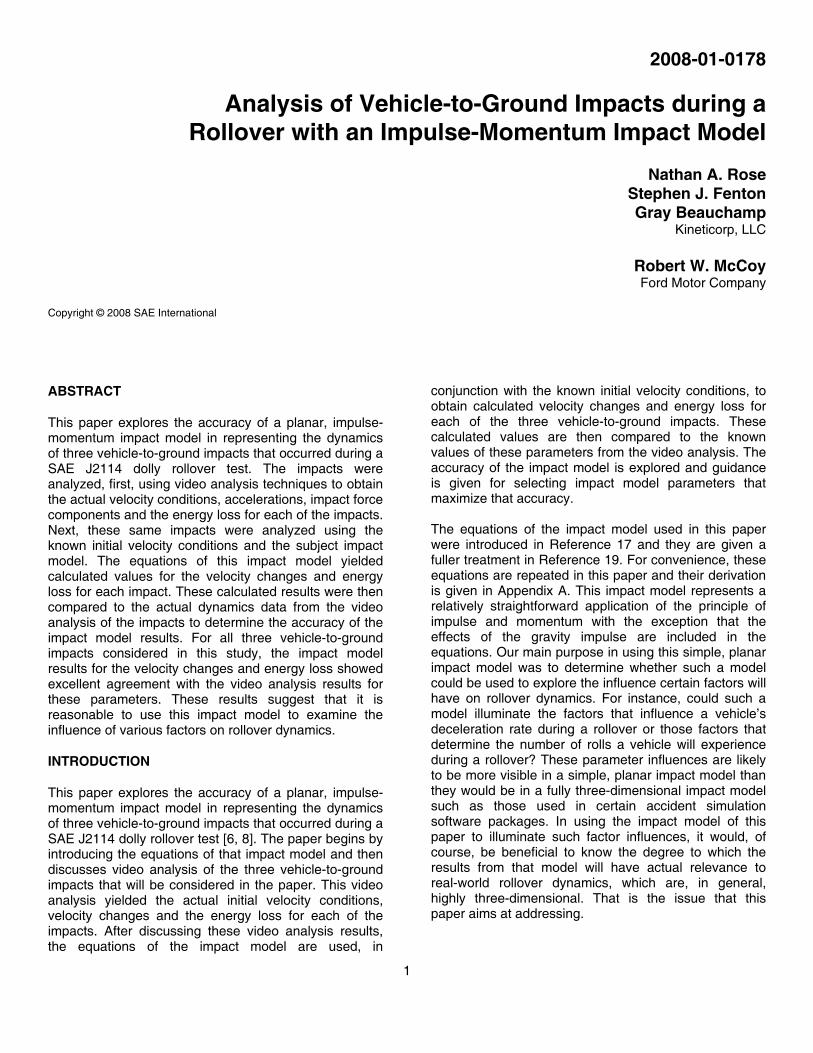
2008-01-0178

Analysis of Vehicle-to-Ground Impacts during a Rollover with an Impulse-Momentum Impact Model

Nathan A. Rose

Stephen J. Fenton Gray Beauchamp

Kineticorp, LLC

Robert W. McCoy Ford Motor Company

Copyright © 2008 SAE International

ABSTRACT

This paper explores the accuracy of a planar, impulse-momentum impact model in representing the dynamics of three vehicle-to-ground impacts that occurred during a SAE J2114 dolly rollover test. The impacts were analyzed, first, using video analysis techniques to obtain the actual velocity conditions, accelerations, impact force components and the energy loss for each of the impacts. Next, these same impacts were analyzed using the known initial velocity conditions and the subject impact model. The equations of this impact model yielded calculated values for the velocity changes and energy loss for each impact. These calculated results were then compared to the actual dynamics data from the video analysis of the impacts to determine the accuracy of the impact model results. For all three vehicle-to-ground impacts considered in this study, the impact model results for the velocity changes and energy loss showed excellent agreement with the video analysis results for these parameters. These results suggest that it is reasonable to use this impact model to examine the influence of various factors on rollover dynamics. INTRODUCTION

This paper explores the accuracy of a planar, impulse-momentum impact model in representing the dynamics of three vehicle-to-ground impacts that occurred during a SAE J2114 dolly rollover test [6, 8]. The paper begins by introducing the equations of that impact model and then discusses video analysis of the three vehicle-to-ground impacts that will be considered in the paper. This video analysis yielded the actual initial velocity conditions, velocity changes and the energy loss for each of the impacts. After discussing these video analysis results, the equations of the impact model are used, in

conjunction with the known initial velocity conditions, to obtain calculated velocity changes and energy loss for each of the three vehicle-to-ground impacts. These calculated values are then compared to the known values of these parameters from the video analysis. The accuracy of the impact model is explored and guidance is given for selecting impact model parameters that maximize that accuracy. The equations of the impact model used in this paper were introduced in Reference 17 and they are given a fuller treatment in Reference 19. For convenience, these equations are repeated in this paper and their derivation is given in Appendix A. This impact model represents a relatively straightforward application of the principle of impulse and momentum with the exception that the effects of the gravity impulse are included in the equations. Our main purpose in using this simple, planar impact model was to determine whether such a model could be used to explore the influence certain factors will have on rollover dynamics. For instance, could such a model illuminate the factors that influence a vehicle’s deceleration rate during a rollover or those factors that determine the number of rolls a vehicle will experience during a rollover? These parameter influences are likely to be more visible in a simple, planar impact model than they would be in a fully three-dimensional impact model such as those used in certain accident simulation software packages. In using the impact model of this paper to illuminate such factor influences, it would, of course, be beneficial to know the degree to which the results from that model will have actual relevance to real-world rollover dynamics, which are, in general, highly three-dimensional. That is the issue that this paper aims at addressing.

2

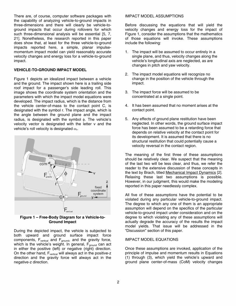
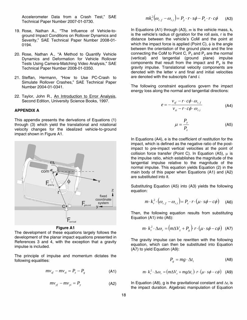
There are, of course, computer software packages with the capability of analyzing vehicle-to-ground impacts in three-dimensions and there will clearly be vehicle-to-ground impacts that occur during rollovers for which such three-dimensional analysis will be essential [5, 7, 21]. Nonetheless, the research reported in this paper does show that, at least for the three vehicle-to-ground impacts reported here, a simple, planar impulse-momentum impact model can yield reasonably accurate velocity changes and energy loss for a vehicle-to-ground impact. VEHICLE-TO-GROUND IMPACT MODEL Figure 1 depicts an idealized impact between a vehicle and the ground. The impact shown here is a trailing side roof impact for a passenger’s side leading roll. This image shows the coordinate system orientation and the parameters with which the impact model equations were developed. The impact radius, which is the distance from the vehicle center-of-mass to the contact point C, is designated with the symbol r. The impact angle, which is the angle between the ground plane and the impact radius, is designated with the symbol φ. The vehicle’s velocity vector is designated with the letter v and the vehicle’s roll velocity is designated ωr.

Figure 1 – Free-Body Diagram for a Vehicle-to-

Ground Impact During the depicted impact, the vehicle is subjected to both upward and ground surface impact force components, Fvertical and Fground, and the gravity force, which is the vehicle’s weight. In general, Fground can act in either the positive (left) or negative (right) direction. On the other hand, Fvertical will always act in the positive-z direction and the gravity force will always act in the negative-z direction.

IMPACT MODEL ASSUMPTIONS Before discussing the equations that will yield the velocity changes and energy loss for the impact of Figure 1, consider the assumptions that the mathematics of those equations will invoke. These assumptions include the following: 1. The impact will be assumed to occur entirely in a

single plane, and thus, velocity changes along the vehicle’s longitudinal axis are neglected, as are changes in pitch and yaw velocity.

2. The impact model equations will recognize no

change in the position of the vehicle through the impact.

3. The impact force will be assumed to be

concentrated at a single point. 4. It has been assumed that no moment arises at the

contact point. 5. Any effects of ground plane restitution have been

neglected. In other words, the ground surface impact force has been assumed to be a retarding force that depends on relative velocity at the contact point for its development. It is assumed that there is no structural restitution that could potentially cause a velocity reversal in the contact region.

The meaning of the first three of these assumptions should be relatively clear. We suspect that the meaning of the last two will be less clear, and thus, we refer the reader to the extensive discussion of these concepts in the text by Brach, titled Mechanical Impact Dynamics [2]. Relaxing these last two assumptions is possible. However, in our judgment, this would make the modeling reported in this paper needlessly complex. All five of these assumptions have the potential to be violated during any particular vehicle-to-ground impact. The degree to which any one of them is an appropriate assumption will depend on the specifics of the particular vehicle-to-ground impact under consideration and on the degree to which violating any of these assumptions will actually degrade the accuracy of the results the impact model yields. That issue will be addressed in the “Discussion” section of this paper. IMPACT MODEL EQUATIONS Once these assumptions are invoked, application of the principle of impulse and momentum results in Equations (1) through (3), which yield the vehicle’s upward and ground plane center-of-mass (CoM) velocity changes

3

and the vehicle’s change in roll velocity.1 Appendix A contains a full derivation of these equations. In these equations, vzc,i is the vertical velocity of the vehicle at Point C immediately preceding the ground contact, kr is the vehicle’s radius of gyration for the roll axis, g is the gravitational constant, Δti is the duration of the impact, and the letters s and c designate the sine and cosine. Note that although it is assumed that the vehicle position does not change during the impact, accounting for the effect of the gravity impulse has required inclusion of the impact duration [9].

( ) ( )⎭⎬⎫

⎩⎨⎧

⋅⋅−+⋅⋅+−=Δ

φφμφ cscrkk

veVr

rizcz 222

2

,1

( )( )⎭⎬

⎫

⎩⎨⎧

⋅⋅−+⋅⋅−

⋅Δ⋅−φφμφ

φφμφcscrk

cscrtgr

i 222

22

( )

itgzVVy Δ⋅+Δ⋅=Δ μ

( ) ( )2r

izr kcsrtgV φφμω −⋅⋅

⋅Δ⋅+Δ=Δ

Examination of Equations (1) through (3) reveals that the initial downward velocity at the Point C (vzc,i) directly influences the velocity changes that occur during the impact, with the velocity changes increasing as this velocity increases. This initial vertical velocity at Point C, which is given by the following equation, is related to the vehicle’s CoM vertical velocity, its roll velocity and the impact angle and radius:

irizizc crvv ,,, ωφ ⋅⋅−=

In this equation, vzi is the vehicle’s vertical velocity at its CoM immediately preceding the impact. Equations (1) through (3) also include the coefficient of restitution, e, and the impulse ratio, μ. The coefficient of restitution is the negative ratio of the post-impact to the pre-impact vertical velocity at Point C. The impulse ratio is the ratio of the ground surface collision impulse to the vertical direction collision impulse. In some instances, the impulse ratio can be thought of as a coulomb friction value, though its application is not limited to this interpretation [2, 3, 4, 14, 19]. In addition to the effects of friction between the ground and the vehicle body, the ground plane impulse may also include the effects of forces generated by snagging between the vehicle and the ground. When such snagging occurs, the impulse

1 The authors presented these equations in Reference 17. However, in that reference, Equation (2) failed to include the gravity term.

ratio should be set at a value that incorporates that snagging. Within this impact model, the sign of the impulse ratio governs the direction in which the ground plane collision force acts. A positive impulse ratio produces a ground plane force that acts in the positive direction and a negative impulse ratio results in a ground plane force that acts in the negative direction. The direction of the ground surface impact force, in turn, determines whether the vehicle will experience a positive or negative ground plane velocity change and whether the ground surface impact force will tend to increase or decrease the roll velocity. Also, note that for a passenger’s side leading roll, as depicted in the image above, the ground speed will be negative, the roll velocity positive, and the impact angle will always be less than 90 degrees. For a driver’s side leading roll, like the crash test analyzed in this paper, the same impact model equations apply, but the ground speed will be positive, the roll velocity negative and the impact angle will always be greater than 90 degrees. The energy loss that occurs during the vehicle-to-ground impact of Figure 1 can be written as follows:

( )2,

22,

22222

2 frrirrtfyizfzi kkvvvvmE ωω −+−+−⋅=Δ

The energy loss of Equation (5) includes the energy loss due to vehicle deformation, ground deformation, and sliding, snagging or furrowing between the vehicle structure and the ground.

ROLLOVER CRASH TEST SETUP

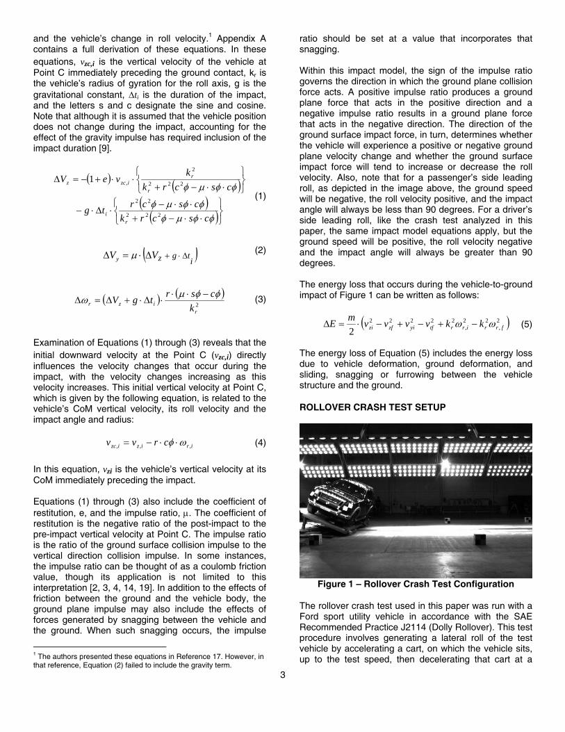
Figure 1 – Rollover Crash Test Configuration

The rollover crash test used in this paper was run with a Ford sport utility vehicle in accordance with the SAE Recommended Practice J2114 (Dolly Rollover). This test procedure involves generating a lateral roll of the test vehicle by accelerating a cart, on which the vehicle sits, up to the test speed, then decelerating that cart at a

(1)

(2)

(3)

(4)

(5)

4

sufficient rate to initiate the rollover. The vehicle is situated on the cart perpendicular to the initial velocity direction with an initial roll angle of 23 degrees. In the test under consideration in this paper, the vehicle was situated on the cart with its driver’s side leading and the cart and test vehicle were accelerated up to a speed of approximately 31 mph before the cart deceleration was initiated. Figure 1 shows the test vehicle just before it began exiting the cart.

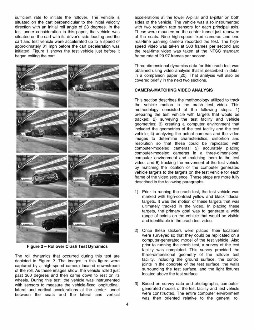
Figure 2 – Rollover Crash Test Dynamics

The roll dynamics that occurred during this test are depicted in Figure 2. The images in this figure were captured by a high-speed camera located downstream of the roll. As these images show, the vehicle rolled just past 360 degrees and then came down to rest on its wheels. During this test, the vehicle was instrumented with sensors to measure the vehicle-fixed longitudinal, lateral and vertical accelerations at the center tunnel between the seats and the lateral and vertical

accelerations at the lower A-pillar and B-pillar on both sides of the vehicle. The vehicle was also instrumented with two rotation rate sensors for each principal axis. These were mounted on the center tunnel just rearward of the seats. Nine high-speed fixed cameras and one real-time panning camera recorded the test. The high-speed video was taken at 500 frames per second and the real-time video was taken at the NTSC standard frame rate of 29.97 frames per second.

Three-dimensional dynamics data for this crash test was obtained using video analysis that is described in detail in a companion paper [20]. That analysis will also be covered briefly in the next two sections.

CAMERA-MATCHING VIDEO ANALYSIS

This section describes the methodology utilized to track the vehicle motion in the crash test video. This methodology consisted of the following steps: 1) preparing the test vehicle with targets that would be tracked; 2) surveying the test facility and vehicle geometries; 3) creating a computer environment that included the geometries of the test facility and the test vehicle; 4) analyzing the actual cameras and the video images to determine characteristics, distortion and resolution so that these could be replicated with computer-modeled cameras; 5) accurately placing computer-modeled cameras in a three-dimensional computer environment and matching them to the test video; and 6) tracking the movement of the test vehicle by matching the location of the computer generated vehicle targets to the targets on the test vehicle for each frame of the video sequence. These steps are more fully described in the following paragraphs.

1) Prior to running the crash test, the test vehicle was marked with high-contrast yellow and black fiducial targets. It was the motion of these targets that was ultimately tracked in the video. In placing these targets, the primary goal was to generate a wide range of points on the vehicle that would be visible and identifiable in the crash test video.

2) Once these stickers were placed, their locations were surveyed so that they could be replicated on a computer-generated model of the test vehicle. Also prior to running the crash test, a survey of the test facility was completed. This survey provided the three-dimensional geometry of the rollover test facility, including the ground surface, the control joints in the concrete of the test surface, the walls surrounding the test surface, and the light fixtures located above the test surface.

3) Based on survey data and photographs, computer-generated models of the test facility and test vehicle were constructed. The entire computer environment was then oriented relative to the general roll

5

direction. With the survey of the test vehicle aligned to the computer model, the target stickers that were placed on the test vehicle, and subsequently surveyed, could be transferred to identical locations on the computer model of the vehicle. These target locations were used to track the motion of the test vehicle.

4) The optical and geometric characteristics of all the cameras were documented and analyzed in order to create computer-generated cameras that mimicked each individual camera that captured video of the rollover test. The data for these cameras came from the survey of these cameras, analysis of the sensors, and analysis of the technical and specification drawings. Each camera was created according to its specific characteristics, since these characteristics differed between cameras. These computer-modeled cameras were also located and oriented to be identical to the cameras surveyed at the facility at the time the dolly rollover test was conducted.

5) Having created a computer-modeled environment that contained the geometry of the test facility, the test vehicle and a series of computer-modeled cameras that replicate the actual cameras, test video from each camera was then designated as a background image for its corresponding computer-modeled camera. Each computer-modeled camera could then be used to simultaneously view the computer model of the test facility and the crash test

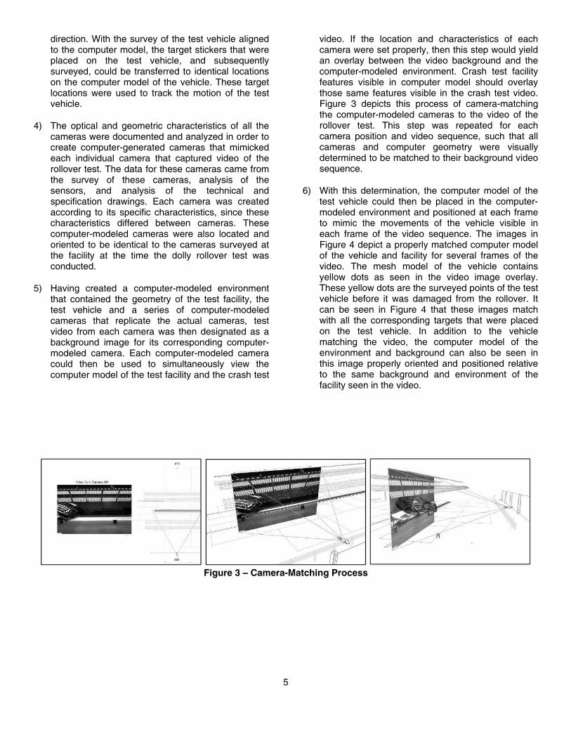
video. If the location and characteristics of each camera were set properly, then this step would yield an overlay between the video background and the computer-modeled environment. Crash test facility features visible in computer model should overlay those same features visible in the crash test video. Figure 3 depicts this process of camera-matching the computer-modeled cameras to the video of the rollover test. This step was repeated for each camera position and video sequence, such that all cameras and computer geometry were visually determined to be matched to their background video sequence.

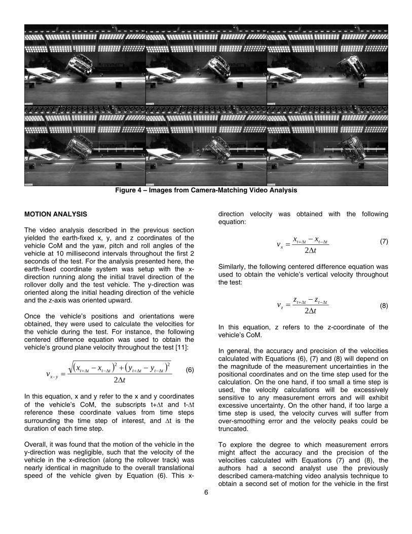
6) With this determination, the computer model of the test vehicle could then be placed in the computer-modeled environment and positioned at each frame to mimic the movements of the vehicle visible in each frame of the video sequence. The images in Figure 4 depict a properly matched computer model of the vehicle and facility for several frames of the video. The mesh model of the vehicle contains yellow dots as seen in the video image overlay. These yellow dots are the surveyed points of the test vehicle before it was damaged from the rollover. It can be seen in Figure 4 that these images match with all the corresponding targets that were placed on the test vehicle. In addition to the vehicle matching the video, the computer model of the environment and background can also be seen in this image properly oriented and positioned relative to the same background and environment of the facility seen in the video.

Figure 3 – Camera-Matching Process

6

Figure 4 – Images from Camera-Matching Video Analysis

MOTION ANALYSIS

The video analysis described in the previous section yielded the earth-fixed x, y, and z coordinates of the vehicle CoM and the yaw, pitch and roll angles of the vehicle at 10 millisecond intervals throughout the first 2 seconds of the test. For the analysis presented here, the earth-fixed coordinate system was setup with the x- direction running along the initial travel direction of the rollover dolly and the test vehicle. The y-direction was oriented along the initial heading direction of the vehicle and the z-axis was oriented upward.

Once the vehicle’s positions and orientations were obtained, they were used to calculate the velocities for the vehicle during the test. For instance, the following centered difference equation was used to obtain the vehicle’s ground plane velocity throughout the test [11]:

( ) ( )t

yyxxv tttttttt

yx Δ−+−

= Δ−Δ+Δ−Δ+− 2

22

In this equation, x and y refer to the x and y coordinates of the vehicle’s CoM, the subscripts t+Δt and t-Δt reference these coordinate values from time steps surrounding the time step of interest, and Δt is the duration of each time step.

Overall, it was found that the motion of the vehicle in the y-direction was negligible, such that the velocity of the vehicle in the x-direction (along the rollover track) was nearly identical in magnitude to the overall translational speed of the vehicle given by Equation (6). This x-

direction velocity was obtained with the following equation:

txxv tttt

x Δ−

= Δ−Δ+

2

Similarly, the following centered difference equation was used to obtain the vehicle’s vertical velocity throughout the test:

tzzv tttt

z Δ−

= Δ−Δ+

2

In this equation, z refers to the z-coordinate of the vehicle’s CoM.

In general, the accuracy and precision of the velocities calculated with Equations (6), (7) and (8) will depend on the magnitude of the measurement uncertainties in the positional coordinates and on the time step used for the calculation. On the one hand, if too small a time step is used, the velocity calculations will be excessively sensitive to any measurement errors and will exhibit excessive uncertainty. On the other hand, if too large a time step is used, the velocity curves will suffer from over-smoothing error and the velocity peaks could be truncated.

To explore the degree to which measurement errors might affect the accuracy and the precision of the velocities calculated with Equations (7) and (8), the authors had a second analyst use the previously described camera-matching video analysis technique to obtain a second set of motion for the vehicle in the first

(6)

(8)

(7)

7

two seconds of the test, at time increments of 30 milliseconds. The positions and orientations of the vehicle obtained with this second analysis were then compared to the positions and orientations of the vehicle obtained by the first analyst. Overall, the two sets of motion data had an average difference in the x-coordinate of 0.35 inches, with a standard deviation of 0.36 inches, and an average difference in the z-coordinate of 0.42 inches, with a standard deviation of 0.28 inches. Thus, 84% of the time, the difference between the two analysts’ positions was less than 0.71 inches. At least 96% of the time, the difference between the two analysts’ positions was less than 1.0 inch.

Using differential calculus to perform an error analysis [22], it can be shown that the uncertainty in the velocities of Equations (7) and (8) can be estimated with the following equations:

txvxΔ⋅

=2δδ

tzvzΔ⋅

=2δδ

In these equations, δx and δz are the positional uncertainties in the x and z coordinate directions and δvx and δvz are the velocity uncertainties in these same directions. In formulating Equations (9) and (10), it has been assumed that the potential measurement error at each time step is independent of those at the surrounding time steps.

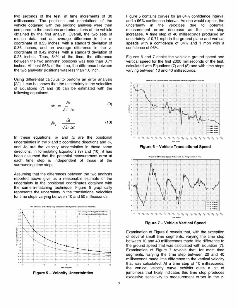
Assuming that the differences between the two analysts reported above give us a reasonable estimate of the uncertainty in the positional coordinates obtained with the camera-matching technique, Figure 5 graphically represents the uncertainty in the translational velocities for time steps varying between 10 and 50 milliseconds.

Figure 5 – Velocity Uncertainties

Figure 5 contains curves for an 84% confidence interval and a 96% confidence interval. As one would expect, the uncertainty in the velocities due to potential measurement errors decrease as the time step increases. A time step of 40 milliseconds produced an uncertainty of 0.71 mph in the ground plane and vertical speeds with a confidence of 84% and 1 mph with a confidence of 96%.

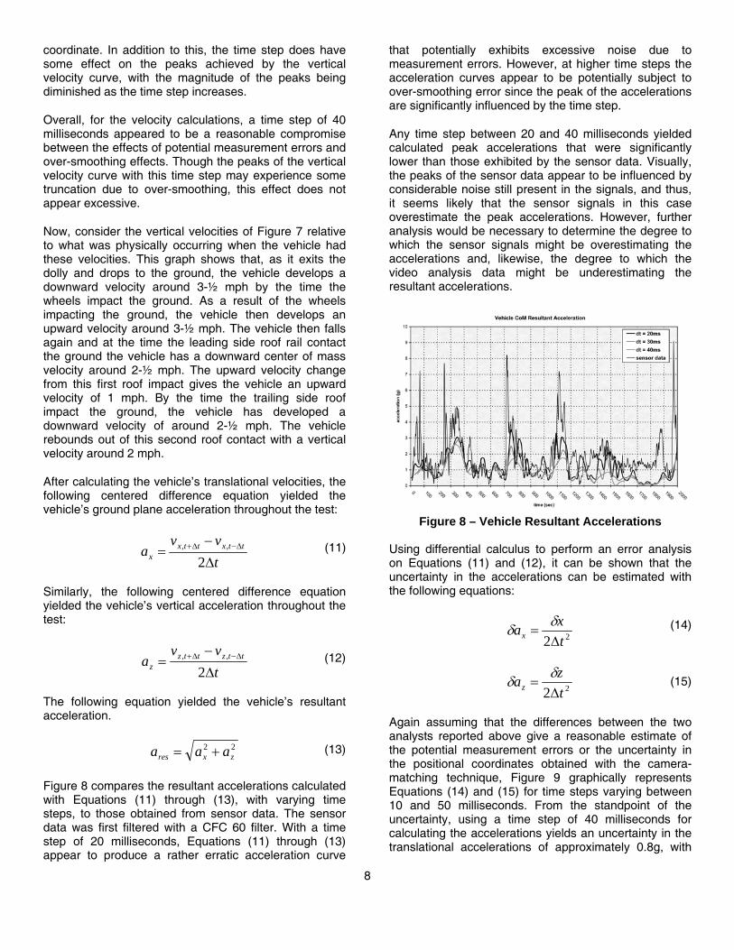
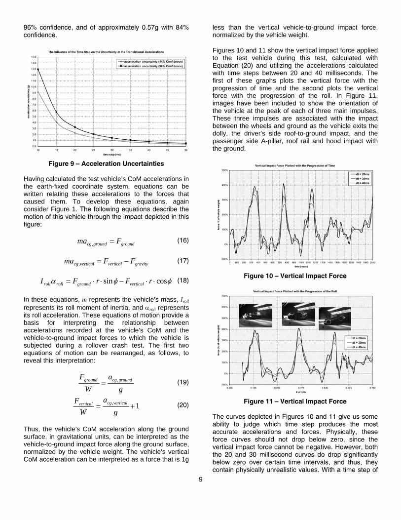
Figures 6 and 7 depict the vehicle’s ground speed and vertical speed for the first 2000 milliseconds of the test, calculated with Equations (7) and (8) and with time steps varying between 10 and 40 milliseconds.

Figure 6 – Vehicle Translational Speed

Figure 7 – Vehicle Vertical Speed

Examination of Figure 6 reveals that, with the exception of several small time segments, varying the time step between 10 and 40 milliseconds made little difference to the ground speed that was calculated with Equation (7). Examination of Figure 7 reveals that, for most time segments, varying the time step between 20 and 40 milliseconds made little difference to the vertical velocity that was calculated. At a time step of 10 milliseconds, the vertical velocity curve exhibits quite a bit of jumpiness that likely indicates this time step produces excessive sensitivity to measurement errors in the z-

(9)

(10)

8

coordinate. In addition to this, the time step does have some effect on the peaks achieved by the vertical velocity curve, with the magnitude of the peaks being diminished as the time step increases.

Overall, for the velocity calculations, a time step of 40 milliseconds appeared to be a reasonable compromise between the effects of potential measurement errors and over-smoothing effects. Though the peaks of the vertical velocity curve with this time step may experience some truncation due to over-smoothing, this effect does not appear excessive.

Now, consider the vertical velocities of Figure 7 relative to what was physically occurring when the vehicle had these velocities. This graph shows that, as it exits the dolly and drops to the ground, the vehicle develops a downward velocity around 3-½ mph by the time the wheels impact the ground. As a result of the wheels impacting the ground, the vehicle then develops an upward velocity around 3-½ mph. The vehicle then falls again and at the time the leading side roof rail contact the ground the vehicle has a downward center of mass velocity around 2-½ mph. The upward velocity change from this first roof impact gives the vehicle an upward velocity of 1 mph. By the time the trailing side roof impact the ground, the vehicle has developed a downward velocity of around 2-½ mph. The vehicle rebounds out of this second roof contact with a vertical velocity around 2 mph.

After calculating the vehicle’s translational velocities, the following centered difference equation yielded the vehicle’s ground plane acceleration throughout the test:

tvv

a ttxttxx Δ

−= Δ−Δ+

2,,

Similarly, the following centered difference equation yielded the vehicle’s vertical acceleration throughout the test:

tvv

a ttzttzz Δ

−= Δ−Δ+

2,,

The following equation yielded the vehicle’s resultant acceleration.

22zxres aaa +=

Figure 8 compares the resultant accelerations calculated with Equations (11) through (13), with varying time steps, to those obtained from sensor data. The sensor data was first filtered with a CFC 60 filter. With a time step of 20 milliseconds, Equations (11) through (13) appear to produce a rather erratic acceleration curve

that potentially exhibits excessive noise due to measurement errors. However, at higher time steps the acceleration curves appear to be potentially subject to over-smoothing error since the peak of the accelerations are significantly influenced by the time step.

Any time step between 20 and 40 milliseconds yielded calculated peak accelerations that were significantly lower than those exhibited by the sensor data. Visually, the peaks of the sensor data appear to be influenced by considerable noise still present in the signals, and thus, it seems likely that the sensor signals in this case overestimate the peak accelerations. However, further analysis would be necessary to determine the degree to which the sensor signals might be overestimating the accelerations and, likewise, the degree to which the video analysis data might be underestimating the resultant accelerations.

Figure 8 – Vehicle Resultant Accelerations

Using differential calculus to perform an error analysis on Equations (11) and (12), it can be shown that the uncertainty in the accelerations can be estimated with the following equations:

22 txax Δ

=δδ

22 tzaz Δ

=δδ

Again assuming that the differences between the two analysts reported above give a reasonable estimate of the potential measurement errors or the uncertainty in the positional coordinates obtained with the camera-matching technique, Figure 9 graphically represents Equations (14) and (15) for time steps varying between 10 and 50 milliseconds. From the standpoint of the uncertainty, using a time step of 40 milliseconds for calculating the accelerations yields an uncertainty in the translational accelerations of approximately 0.8g, with

(12)

(13)

(11)

(14)

(15)

9

96% confidence, and of approximately 0.57g with 84% confidence.

Figure 9 – Acceleration Uncertainties

Having calculated the test vehicle’s CoM accelerations in the earth-fixed coordinate system, equations can be written relating these accelerations to the forces that caused them. To develop these equations, again consider Figure 1. The following equations describe the motion of this vehicle through the impact depicted in this figure:

groundgroundcg Fma =,

gravityverticalverticalcg FFma −=,

φφα cossin ⋅⋅−⋅⋅= rFrFI verticalgroundrollroll In these equations, m represents the vehicle’s mass, Iroll represents its roll moment of inertia, and αroll represents its roll acceleration. These equations of motion provide a basis for interpreting the relationship between accelerations recorded at the vehicle’s CoM and the vehicle-to-ground impact forces to which the vehicle is subjected during a rollover crash test. The first two equations of motion can be rearranged, as follows, to reveal this interpretation:

ga

WF groundcgground ,=

1, +=g

aW

F verticalcgvertical

Thus, the vehicle’s CoM acceleration along the ground surface, in gravitational units, can be interpreted as the vehicle-to-ground impact force along the ground surface, normalized by the vehicle weight. The vehicle’s vertical CoM acceleration can be interpreted as a force that is 1g

less than the vertical vehicle-to-ground impact force, normalized by the vehicle weight.

Figures 10 and 11 show the vertical impact force applied to the test vehicle during this test, calculated with Equation (20) and utilizing the accelerations calculated with time steps between 20 and 40 milliseconds. The first of these graphs plots the vertical force with the progression of time and the second plots the vertical force with the progression of the roll. In Figure 11, images have been included to show the orientation of the vehicle at the peak of each of three main impulses. These three impulses are associated with the impact between the wheels and ground as the vehicle exits the dolly, the driver’s side roof-to-ground impact, and the passenger side A-pillar, roof rail and hood impact with the ground.

Figure 10 – Vertical Impact Force

Figure 11 – Vertical Impact Force

The curves depicted in Figures 10 and 11 give us some ability to judge which time step produces the most accurate accelerations and forces. Physically, these force curves should not drop below zero, since the vertical impact force cannot be negative. However, both the 20 and 30 millisecond curves do drop significantly below zero over certain time intervals, and thus, they contain physically unrealistic values. With a time step of

(16)

(17)

(18)

(19)

(20)

10

40 milliseconds, these unrealistic negative impact force values are nearly eliminated. This gives one indication that the forces calculated with the 40 millisecond time interval are likely more accurate than those calculated with a 20 or 30 millisecond time interval. It is also likely an indication that the sensor accelerations of Figure 8 are overestimating the peak accelerations since these accelerations are directly related to the contact forces. Were these sensor accelerations used to calculate forces, they would no doubt produce peak forces well above those calculated with the video analysis at a time step of 40 milliseconds.

On the other hand, review of the test video appears to show that using a 40 millisecond time step to calculate the vertical impact force results in impact durations that are too long. For instance, for the first wheel-to-ground impact, the 40ms force curve indicates the impact occurred over the time interval from 130 to 490 milliseconds. Review of the video reveals that this impact actually occurred over the interval of time from 225 to 450 milliseconds. Thus, the 40ms force curve implies an impact duration of 360ms for an impact that actually only lasted for approximately 225 milliseconds. In terms of the impact duration, then, the 20 and 30 millisecond force curves provide a better estimate of the overall impact durations.

Impact duration aside, given that the 40ms curve doesn’t contain the physically unrealistic negative force values that the 20 and 30 ms curve do, the 40ms curve may still provide the most reasonable estimate of the peak impact forces. If that is the case, then the first wheel-to-ground impact produced a peak vertical impact force that was approximately 335% of the vehicle weight and both the driver’s side and passenger’s side roof impacts produced peak vertical impact forces of approximately 270% of the vehicle weight.

Now, consider the vehicle’s roll velocity. The following difference equation will yield the vehicle’s average roll velocity over two time steps:

tttrttr

r Δ−

= Δ−Δ+

2,, θθ

ω

In Equation (21), θr is the vehicle roll angle at the specified time step. Similar equations could be written for obtaining the vehicle’s pitch and yaw velocities.

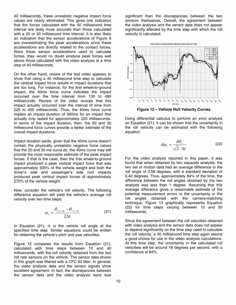
Figure 12 compares the results from Equation (21), calculated with time steps between 10 and 40 milliseconds, with the roll velocity obtained from the two roll rate sensors on the vehicle. The sensor data shown in this graph was filtered with a CFC 60 filter. In general, the video analysis data and the sensor signals show excellent agreement. In fact, the discrepancies between the sensor data and the video analysis were less

significant than the discrepancies between the two sensors themselves. Overall, the agreement between the video analysis and the sensor data does not appear significantly affected by the time step with which the roll velocity is calculated.

Figure 12 – Vehicle Roll Velocity Curves

Using differential calculus to perform an error analysis on Equation (21), it can be shown that the uncertainty in the roll velocity can be estimated with the following equation:

tr

rΔ⋅

=2δθδω

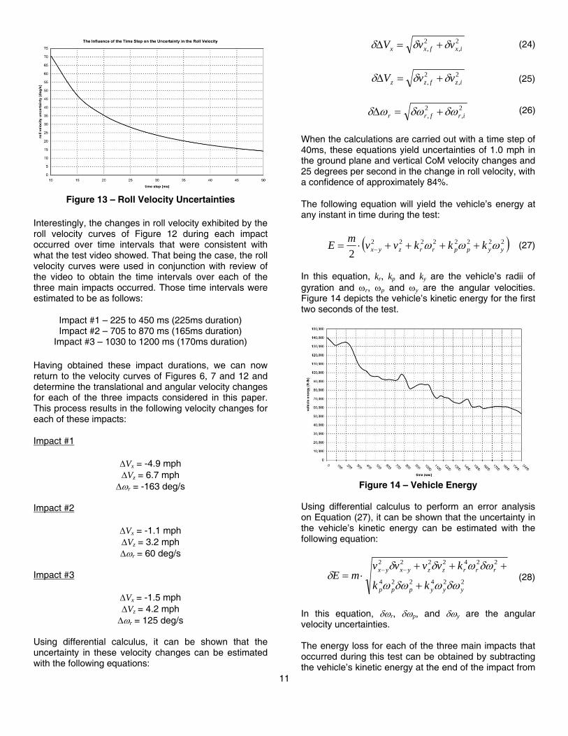
For the video analysis reported in this paper, it was found that when obtained by two separate analysts, the two set of motion data had an average difference in the roll angle of 0.58 degrees, with a standard deviation of 0.40 degrees. Thus, approximately 84% of the time, the difference between the roll angles obtained by the two analysts was less than 1 degree. Assuming that this average difference gives a reasonable estimate of the potential measurement errors or the uncertainty in the roll angles obtained with the camera-matching technique, Figure 13 graphically represents Equation (22) for time steps varying between 10 and 50 milliseconds.

Since the agreement between the roll velocities obtained with video analysis and the sensor data does not appear to depend significantly on the time step used to calculate the roll velocity, a 40 millisecond time step again seems a good choice for use in the video analysis calculations. At this time step, the uncertainty in the calculated roll velocities will be around 18 degrees per second, with a confidence of 84%.

(21)

(22)

11

Figure 13 – Roll Velocity Uncertainties

Interestingly, the changes in roll velocity exhibited by the roll velocity curves of Figure 12 during each impact occurred over time intervals that were consistent with what the test video showed. That being the case, the roll velocity curves were used in conjunction with review of the video to obtain the time intervals over each of the three main impacts occurred. Those time intervals were estimated to be as follows:

Impact #1 – 225 to 450 ms (225ms duration) Impact #2 – 705 to 870 ms (165ms duration)

Impact #3 – 1030 to 1200 ms (170ms duration)

Having obtained these impact durations, we can now return to the velocity curves of Figures 6, 7 and 12 and determine the translational and angular velocity changes for each of the three impacts considered in this paper. This process results in the following velocity changes for each of these impacts:

Impact #1

ΔVx = -4.9 mph ΔVz = 6.7 mph

Δωr = -163 deg/s

Impact #2

ΔVx = -1.1 mph ΔVz = 3.2 mph Δωr = 60 deg/s

Impact #3

ΔVx = -1.5 mph ΔVz = 4.2 mph Δωr = 125 deg/s

Using differential calculus, it can be shown that the uncertainty in these velocity changes can be estimated with the following equations:

2,

2, ixfxx vvV δδδ +=Δ

2,

2, izfzz vvV δδδ +=Δ

2,

2, irfrr δωδωωδ +=Δ

When the calculations are carried out with a time step of 40ms, these equations yield uncertainties of 1.0 mph in the ground plane and vertical CoM velocity changes and 25 degrees per second in the change in roll velocity, with a confidence of approximately 84%.

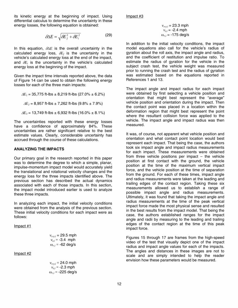
The following equation will yield the vehicle’s energy at any instant in time during the test:

( )22222222

2 yypprrzyx kkkvvmE ωωω ++++⋅= −

In this equation, kr, kp and ky are the vehicle’s radii of gyration and ωr, ωp and ωy are the angular velocities. Figure 14 depicts the vehicle’s kinetic energy for the first two seconds of the test.

Figure 14 – Vehicle Energy

Using differential calculus to perform an error analysis on Equation (27), it can be shown that the uncertainty in the vehicle’s kinetic energy can be estimated with the following equation:

224224

2242222

yyyppp

rrrzzyxyx

kk

kvvvvmE

δωωδωω

δωωδδδ

+

+++⋅=

−−

In this equation, δωr, δωp, and δωy are the angular velocity uncertainties. The energy loss for each of the three main impacts that occurred during this test can be obtained by subtracting the vehicle’s kinetic energy at the end of the impact from

(27)

(25)

(26)

(28)

(24)

12

its kinetic energy at the beginning of impact. Using differential calculus to determine the uncertainty in these energy losses, the following equation is obtained:

22if EEE δδδ +=Δ

In this equation, δΔE is the overall uncertainty in the calculated energy loss, δEf is the uncertainty in the vehicle’s calculated energy loss at the end of the impact, and δEi is the uncertainty in the vehicle’s calculated energy loss at the beginning of the impact. Given the impact time intervals reported above, the data of Figure 14 can be used to obtain the following energy losses for each of the three main impacts:

ΔE1 = 35,775 ft-lbs ± 8,219 ft-lbs (27.0% ± 6.2%)

ΔE2 = 8,957 ft-lbs ± 7,262 ft-lbs (9.8% ± 7.9%)

ΔE3 = 13,749 ft-lbs ± 6,932 ft-lbs (16.0% ± 8.1%) The uncertainties reported with these energy losses have a confidence of approximately 84%. These uncertainties are rather significant relative to the best estimate values. Clearly, considerable uncertainty has accrued through the course of these calculations.

ANALYZING THE IMPACTS

Our primary goal in the research reported in this paper was to determine the degree to which a simple, planar, impulse-momentum impact model would accurately yield the translational and rotational velocity changes and the energy loss for the three impacts identified above. The previous section has described the actual dynamics associated with each of those impacts. In this section, the impact model introduced earlier is used to analyze these three impacts.

In analyzing each impact, the initial velocity conditions were obtained from the analysis of the previous section. These initial velocity conditions for each impact were as follows:

Impact #1

vx-y,i = 29.5 mph vz,i = -3.4 mph ωr,i = -62 deg/s

Impact #2

vx-y,i = 24.0 mph vz,i = -2.3 mph ωr,i = -225 deg/s

Impact #3

vx-y,i = 23.3 mph vz,i = -2.4 mph ωr,i = -175 deg/s

In addition to the initial velocity conditions, the impact model equations also call for the vehicle’s radius of gyration about the roll axis, the impact angle and radius, and the coefficient of restitution and impulse ratio. To estimate the radius of gyration for the vehicle in the subject crash test, the vehicle weight was measured prior to running the crash test and the radius of gyration was estimated based on the equations reported in References 1 and 13.

The impact angle and impact radius for each impact were obtained by first selecting a vehicle position and orientation that might best represent the “average” vehicle position and orientation during the impact. Then the contact point was placed in a location within the deformation region that might best represent the point where the resultant collision force was applied to the vehicle. The impact angle and impact radius was then measured.

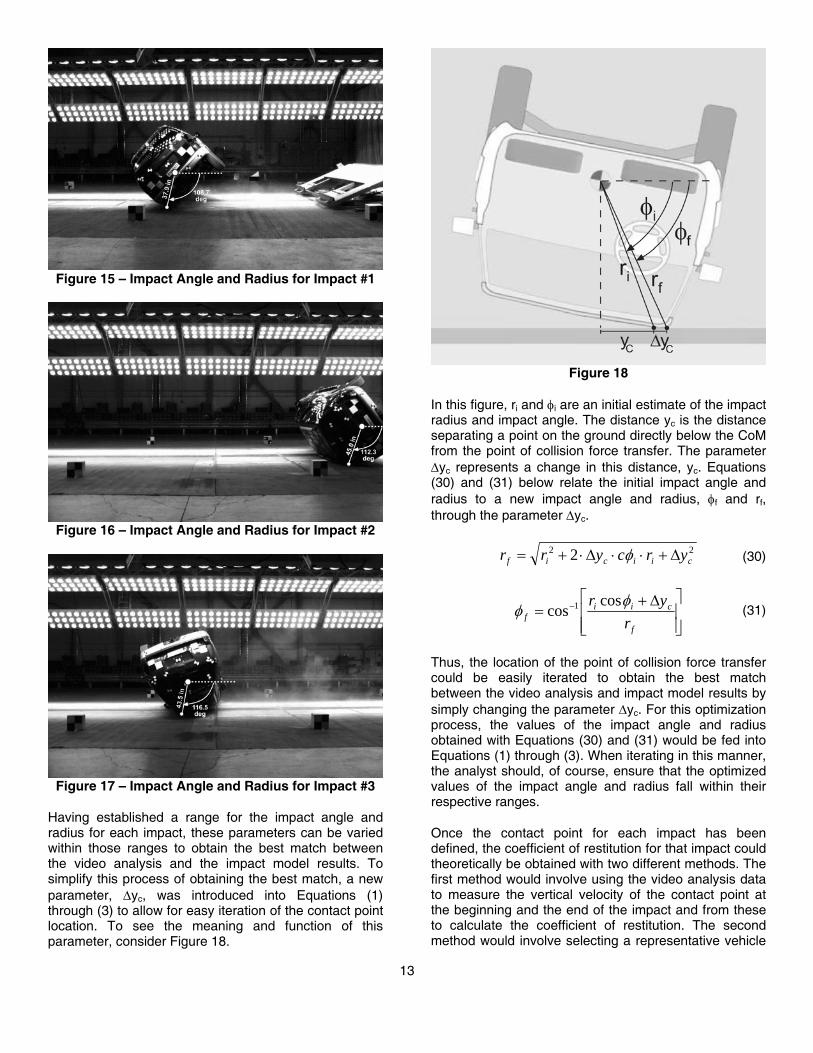
It was, of course, not apparent what vehicle position and orientation and what contact point location would best represent each impact. That being the case, the authors took six impact angle and impact radius measurements for each impact. These measurements were obtained from three vehicle positions per impact – the vehicle position at first contact with the ground, the vehicle position at the time of the maximum vertical impact force, and the vehicle position at the time of separation from the ground. For each of these times, impact angle and radius measurements were taken at the leading and trailing edges of the contact region. Taking these six measurements allowed us to establish a range of possible impact angle and radius measurements. Ultimately, it was found that taking the impact angle and radius measurements at the time of the peak vertical impact force made the most physical sense and resulted in the best results from the impact model. That being the case, the authors established ranges for the impact angle and radii by measuring to the leading and trailing edges of the contact region at the time of this peak impact force.

Figures 15 through 17 are frames from the high-speed video of the test that visually depict one of the impact radius and impact angle values for each of the impacts. The angles and distances in these images are not to scale and are simply intended to help the reader envision how these parameters would be measured.

(29)

13

Figure 15 – Impact Angle and Radius for Impact #1

Figure 16 – Impact Angle and Radius for Impact #2

Figure 17 – Impact Angle and Radius for Impact #3

Having established a range for the impact angle and radius for each impact, these parameters can be varied within those ranges to obtain the best match between the video analysis and the impact model results. To simplify this process of obtaining the best match, a new parameter, Δyc, was introduced into Equations (1) through (3) to allow for easy iteration of the contact point location. To see the meaning and function of this parameter, consider Figure 18.

Figure 18

In this figure, ri and φi are an initial estimate of the impact radius and impact angle. The distance yc is the distance separating a point on the ground directly below the CoM from the point of collision force transfer. The parameter Δyc represents a change in this distance, yc. Equations (30) and (31) below relate the initial impact angle and radius to a new impact angle and radius, φf and rf, through the parameter Δyc.

22 2 ciicif yrcyrr Δ+⋅⋅Δ⋅+= φ

⎥⎥⎦

⎤

⎢⎢⎣

⎡ Δ+= −

f

ciif r

yr φφ

coscos 1

Thus, the location of the point of collision force transfer could be easily iterated to obtain the best match between the video analysis and impact model results by simply changing the parameter Δyc. For this optimization process, the values of the impact angle and radius obtained with Equations (30) and (31) would be fed into Equations (1) through (3). When iterating in this manner, the analyst should, of course, ensure that the optimized values of the impact angle and radius fall within their respective ranges.

Once the contact point for each impact has been defined, the coefficient of restitution for that impact could theoretically be obtained with two different methods. The first method would involve using the video analysis data to measure the vertical velocity of the contact point at the beginning and the end of the impact and from these to calculate the coefficient of restitution. The second method would involve selecting a representative vehicle

(30)

(31)

14

orientation for the impact – in this case, the vehicle orientation at the time of the peak vertical force – and then imposing the assumption that the vehicle orientation does not change during the impact and then calculating the coefficient of restitution based on the initial and final vertical velocities, the initial and final roll velocities, and the impact angle and impact radius.

To understand the difference between these two methods, consider that the coefficient of restitution is defined as the negative ratio of the post-impact to the pre-impact vertical velocity at the point where the resultant collision force is transferred. Since the point of collision force transfer will lie near the perimeter of the vehicle, both the vehicle’s roll velocity and roll orientation can significantly influence to the vertical velocity at Point C at any instant in time. The vehicle’s orientation will determine what component of the vehicle’s perimeter velocity contributes to the vertical velocity at C and in which direction it contributes. The influence of these factors is displayed mathematically in Equation (4).

Now, consider that the impact model equations described above assumed that the vehicle does not move during the impact (instantaneous impact). In reality, even given the relatively short impact durations associated with the impacts considered in this paper, the vehicle traverses a relatively significant roll angle during these impacts. Specifically, in the specific test under consideration here, the vehicle traversed a roll angle of approximately 31 degrees during the first impact, 31-½ degrees during the second impact, and 21 degrees during the third impact.

If one uses the first method for calculating the coefficient of restitution, then the vertical velocity of the contact point at the beginning and the end of the impact will be measured with the impact radius at different angles. This difference is caused by the fact that the vehicle continues to roll throughout the impact. If one uses the second method for calculating the coefficient of restitution, then the vertical velocity of the contact point at the beginning and end of the impact will be calculated with the impact radius at a constant angle (its angle at the time of the peak force). Thus, the first method yields a coefficient of restitution that may cause inaccuracies in the impact model since it violates the instantaneous impact assumption of the model. The second method is more consistent with the modeling assumptions, but it yields a value for the coefficient of restitution that does not reflect the fact that the vehicle rolls throughout the impact. This second way of treating the coefficient of restitution is also most consistent with the way that it has typically been obtained for use with other planar, impulse-momentum impact models [18].

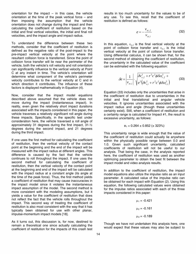
As it turns out, this discussion is, for now, destined to remain a theoretical one since actually calculating the coefficient of restitution for the impacts of this crash test

results in too much uncertainty for the values to be of any use. To see this, recall that the coefficient of restitution is defined as follows:

izc

fzc

vv

e,

,−=

In this equation, vzc,f is the final vertical velocity at the point of collision force transfer and vzc,i is the initial vertical velocity at the point of collision force transfer. Using differential calculus, it can be shown that, for the second method of obtaining the coefficient of restitution, the uncertainty in the calculated value of the coefficient can be estimated with the following equation:

( )2,

222,

2

2,

222,

,

1

iriz

frfz

izc crve

crvv

eφδωδ

φδωδδ

+

++⋅=

Equation (33) includes only the uncertainties that arise in the coefficient of restitution due to uncertainties in the initial and final translational and angular vehicle velocities. It ignores uncertainties associated with the impact radius and angle (though these uncertainties certainly exist). Still, when a coefficient of restitution and a certainty range is calculated for Impact #1, the result is excessive uncertainty, as follows:

e1 = 0.264 ± 0.852 (± 323%)

This uncertainty range is wide enough that the value of the coefficient of restitution could actually lie anywhere within the physically possible range between 0.0 and 1.0. Given such significant uncertainty, calculated coefficients of restitution will not be useful to our analysis. That being the case, in the analysis reported here, the coefficient of restitution was used as another optimizing parameter to obtain the best fit between the impact model and video analysis results.

In addition to the coefficient of restitution, the impact model equations also utilize the impulse ratio as an input parameter. A calculated value of the impulse ratio can be obtained for each impact with Equation (2). Using this equation, the following calculated values were obtained for the impulse ratios associated with each of the three impacts considered in this paper:

μ1 = -0.421

μ2 = -0.161

μ3 = -0.189

Though we have not undertaken this analysis here, one would expect that these values may also be subject to

(32)

(33)

15

considerable uncertainty. That being the case, in the analysis reported below, the authors began by setting the impulse ratio at these calculated values but then changed it as necessary to obtain the best fit solution for the video analysis results. As it turned out, for Impacts 1 and 3, these calculated values did yield the best-fit solution.

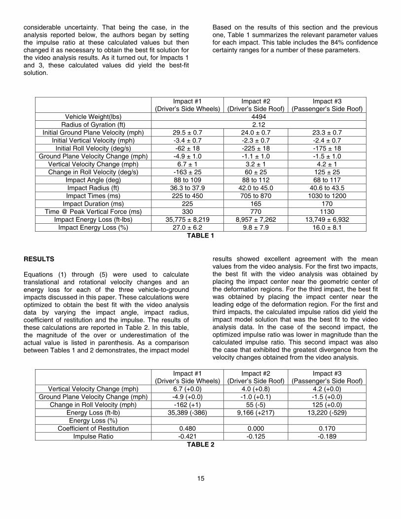
Based on the results of this section and the previous one, Table 1 summarizes the relevant parameter values for each impact. This table includes the 84% confidence certainty ranges for a number of these parameters.

Impact #1 (Driver’s Side Wheels)

Impact #2 (Driver’s Side Roof)

Impact #3 (Passenger’s Side Roof)

Vehicle Weight(lbs) 4494 Radius of Gyration (ft) 2.12

Initial Ground Plane Velocity (mph) 29.5 ± 0.7 24.0 ± 0.7 23.3 ± 0.7 Initial Vertical Velocity (mph) -3.4 ± 0.7 -2.3 ± 0.7 -2.4 ± 0.7 Initial Roll Velocity (deg/s) -62 ± 18 -225 ± 18 -175 ± 18

Ground Plane Velocity Change (mph) -4.9 ± 1.0 -1.1 ± 1.0 -1.5 ± 1.0 Vertical Velocity Change (mph) 6.7 ± 1 3.2 ± 1 4.2 ± 1 Change in Roll Velocity (deg/s) -163 ± 25 60 ± 25 125 ± 25

Impact Angle (deg) 88 to 109 88 to 112 68 to 117 Impact Radius (ft) 36.3 to 37.9 42.0 to 45.0 40.6 to 43.5 Impact Times (ms) 225 to 450 705 to 870 1030 to 1200

Impact Duration (ms) 225 165 170 Time @ Peak Vertical Force (ms) 330 770 1130

Impact Energy Loss (ft-lbs) 35,775 ± 8,219 8,957 ± 7,262 13,749 ± 6,932 Impact Energy Loss (%) 27.0 ± 6.2 9.8 ± 7.9 16.0 ± 8.1

TABLE 1

RESULTS

Equations (1) through (5) were used to calculate translational and rotational velocity changes and an energy loss for each of the three vehicle-to-ground impacts discussed in this paper. These calculations were optimized to obtain the best fit with the video analysis data by varying the impact angle, impact radius, coefficient of restitution and the impulse. The results of these calculations are reported in Table 2. In this table, the magnitude of the over or underestimation of the actual value is listed in parenthesis. As a comparison between Tables 1 and 2 demonstrates, the impact model

results showed excellent agreement with the mean values from the video analysis. For the first two impacts, the best fit with the video analysis was obtained by placing the impact center near the geometric center of the deformation regions. For the third impact, the best fit was obtained by placing the impact center near the leading edge of the deformation region. For the first and third impacts, the calculated impulse ratios did yield the impact model solution that was the best fit to the video analysis data. In the case of the second impact, the optimized impulse ratio was lower in magnitude than the calculated impulse ratio. This second impact was also the case that exhibited the greatest divergence from the velocity changes obtained from the video analysis.

Impact #1 (Driver’s Side Wheels)

Impact #2 (Driver’s Side Roof)

Impact #3 (Passenger’s Side Roof)

Vertical Velocity Change (mph) 6.7 (+0.0) 4.0 (+0.8) 4.2 (+0.0) Ground Plane Velocity Change (mph) -4.9 (+0.0) -1.0 (+0.1) -1.5 (+0.0)

Change in Roll Velocity (mph) -162 (+1) 55 (-5) 125 (+0.0) Energy Loss (ft-lb) 35,389 (-386) 9,166 (+217) 13,220 (-529) Energy Loss (%)

Coefficient of Restitution 0.480 0.000 0.170 Impulse Ratio -0.421 -0.125 -0.189

TABLE 2

16

DISCUSSION Impact Model Assumptions Now, consider the impact model results of Table 2 in relationship to the impact model assumptions. Based on the results of Table 2, it can be concluded that any violation of the impact model assumptions did not significantly degrade the accuracy of the impact model calculations. That result is encouraging and indicates that the simple planar impact model used here can offer insight into rollover dynamics. That said, it still makes sense to be specific about the degree to which certain impact model assumptions were violated and how those violations were dealt with in the modeling. It is, perhaps, obvious that there will be cases where violations of the impact model assumptions will be more significant that what was observed in this test and that, in such cases, the impact model used here will not be useful. Impacts #1 and #2 nearly satisfied the first impact model assumption, which was that the impact occurred entirely in a single plane. At the time of these impacts, the vehicle had experienced very little pitching or yawing and the vehicle velocity was still in line with its initial direction. By the time of Impact #3, the vehicle had developed a relatively significant forward pitch angle with a corresponding forward pitch velocity. Thus, strictly speaking, Impact #3 did violate the planar impact assumption. Despite this, the impact model results for Impact #3 still showed excellent agreement with the video analysis results. Thus, this violation of the planar impact assumption was not fatal to the accuracy of the model. All three impacts violated the second assumption of the impact model, which was that the vehicle experienced no change in position during the impact. As was stated above, the vehicle traversed a roll angle of approximately 31 degrees during the first impact, 31-½ degrees during the second impact, and 21 degrees during the third impact. Overcoming this discrepancy between the impact model assumption and the real impacts appeared to be primarily a matter of determining a vehicle position that was the most representative of the impact. In the case of these three impacts, the vehicle position at the peak vertical force yielded the best impact model results. Clearly, the third assumption of the impact model, that the impact force was applied at a single point would be violated for any real-world impact. Still, overcoming this discrepancy appeared to be primarily a matter of determining a contact point location that was most representative of the point of application of the resultant collision force. As we have already stated, for the first two impacts, the best fit was obtained with the video analysis data by placing the point of collision force transfer near the geometric center of the deformation

region. For the third impact, the best results were obtained by placing the impact center near the leading edge of the contact region. It is unclear to us at this point whether the fourth assumption, that no moment arose at the point of collision force transfer, was violated or not. Further research could explore the influence of a moment at the contact point on the resulting rollover dynamics. At any rate, ignoring such a moment did not adversely affect the impact results to any significant degree. The fifth impact model assumption, that no velocity reversal occurs during the impact, was satisfied for each of the three impacts that were analyzed in this paper. This was determined by reviewing the crash test video. The Larger Context A number of studies that have sought causes of occupant injuries in rollovers have focused on crash attributes or outcomes – the number of quarter rolls [12], the initial vehicle translational speed [15], and the magnitude of roof deformation [10] or post-crash headroom [16] – and on how those attributes correlate to injury rates. However, crash attributes and outcomes are not causes. In fact, they are effects that result from a combination of the rollover initial conditions and the particular forces to which the vehicle is subjected during the rollover. It is these initial conditions and underlying forces that cause certain crash attributes or outcomes to be present. If there is a correlation between certain injury types and a particular crash attribute, it is the underlying forces that cause this crash attribute that could also relate to the actual cause of that injury type. Thus, an understanding of the initial conditions and underlying forces causing certain crash attributes may be significant to reducing injury potential in rollovers. In theory, an impact model such as the one used in this paper could be helpful in understanding the underlying forces and physical relationships that cause certain rollover crash attributes. The impact model used in this paper is simple enough that parameter relationships are not obscured. The equations of the impact model are algebraic, and so, their solution need not be buried within computer code. If one could have confidence that this relatively simple impact model would yield physically realistic and accurate results, then one could conceivable use it to develop an understanding of why certain crash conditions lead to certain crash attributes. That, ultimately, has been the goal of the research reported here: to determine whether this simple, planar impact model would yield accurate, and therefore useful, results for the vehicle-to-ground impact that occur during rollovers. The results reported above are encouraging in this regard. These results suggest that the impact model is capable of yielding accurate results related to the

17

velocity changes and energy loss resulting from a vehicle-to-ground impact. That being the case, it is reasonable to use this impact model to examine the influence of various factors on rollover dynamics. For instance, it can be observed that the rate at which a rolling vehicle decelerates will be determined by the accumulation of the ground plane velocity changes that occur during the rollover. Thus, any factor that influences the ground surface velocity changes will also likely influence the deceleration rate that the vehicle experiences. These factors include the following: (1) the available surface friction, (2) the ground speeds, vertical velocities, and roll velocities experienced during the roll, (3) the orientations of the specific vehicle-to-ground impacts that occur during the roll, (4) the vehicle geometry, (5) and the stiffness of the vehicle structures engaged during the roll. Future research could examine rollover test data and real-world rollovers to determine the degree to which each of these factors might affect a rolling vehicle’s deceleration rate over the course of an entire rollover. CONCLUSIONS • For all three vehicle-to-ground impacts considered in

this study, the impact model results for the velocity changes and energy loss fell within the certainty ranges obtained from the video analysis for these parameters.

• These results suggest that the impact model is

capable of yielding accurate results related to the velocity changes and energy loss resulting from a vehicle-to-ground impact. That being the case, it is reasonable to use this impact model to examine the influence of various factors on rollover dynamics.

REFERENCES 1. Allen, R. Wade, “Estimation of Passenger Vehicle

Inertial Properties and Their Effect on Stability and Handling,” SAE Technical Paper Number 2003-01-0966.

2. Brach, Raymond M., Mechanical Impact Dynamics:

Rigid Body Collisions, Revised Edition, Brach Engineering, 2007.

3. Brach, Raymond M., Brach, R. Matthew, “A Review

of Impact Models for Vehicle Collision,” SAE Technical Paper Number 870048.

4. Brach, Raymond M., Brach, R. Matthew, “Energy

Loss in Vehicle Collisions,” SAE Technical Paper Number 871993.

5. Brandse, Jeroen, “Methodology for Simulation of Rollover Cases,” SAE Technical Paper Number 2006-01-0558.

6. Chou, Clifford C., McCoy, Robert W., Le, Jialiang, “A

Literature Review of Rollover Test Methodologies,” Int. J. Vehicle Safety, Volume 1, Nos. 1/2/3, 2005.

7. Day, Terry D., “Applications and Limitations of 3-

Dimensional Vehicle Rollover Simulation,” SAE Technical Paper Number 2000-01-0852.

8. “Dolly Rollover Recommended Test Procedure,”

Surface Vehicle Recommended Practice J2114, Society of Automotive Engineers, October 1999.

9. Fonda, Albert G., “Nonconservation of Momentum

During Impact,” SAE Technical Paper Number 950355.

10. Friedman, Donald, “Roof Crush Versus Occupant

Injury From 1988 to 1992 Nass,” SAE Technical Paper Number 980210.

11. Hoffman, Joe D., “Numerical Methods for Engineers

and Scientists,” Second Edition, Marcel Dekker, 2001.

12. Hughes, Raymond J., et al., “A Dynamic Test

Procedure for Evaluation of Tripped Rollover Crashes,” SAE Technical Paper Number 2002-01-0693.

13. MacInnis, Duane D., “A Comparison of Moment of

Inertia Estimation Techniques for Vehicle Dynamics Simulation,” SAE Technical Paper Number 970951.

14. Marine, Micky C., “On the Concept of Inter-Vehicle

Friction and Its Application in Automobile Accident Reconstruction,” SAE Technical Paper Number 2007-01-0744.

15. Malliaris, C., “Pivotal Characterization of Car

Rollovers,” Proceedings of the 13th ESV Conference, November 1991.

16. Rains, Glen C., “Determination of the Significance of

Roof Crush on Head and Neck Injury to Passenger Vehicle Occupants in Rollover Crashes,” SAE Technical Paper Number 950655.

17. Rose, Nathan A., Beauchamp, Gray, Fenton,

Stephen J., “Factors Influencing Roof-to-Ground Impact Severity: Video Analysis and Analytical Modeling,” SAE Technical Paper Number 2007-01-0726.

18. Rose, Nathan A., “Quantifying the Uncertainty in the

Coefficient of Restitution Obtained with

18

Accelerometer Data from a Crash Test,” SAE Technical Paper Number 2007-01-0730.

19. Rose, Nathan A., “The Influence of Vehicle-to-

ground Impact Conditions on Rollover Dynamics and Severity,” SAE Technical Paper Number 2008-01-0194.

20. Rose, Nathan A., “A Method to Quantify Vehicle

Dynamics and Deformation for Vehicle Rollover Tests Using Camera-Matching Video Analysis,” SAE Technical Paper Number 2008-01-0350.

21. Steffan, Hermann, “How to Use PC-Crash to

Simulate Rollover Crashes,” SAE Technical Paper Number 2004-01-0341.

22. Taylor, John R., An Introduction to Error Analysis,

Second Edition, University Science Books, 1997. APPENDIX A This appendix presents the derivations of Equations (1) through (3) which yield the translational and rotational velocity changes for the idealized vehicle-to-ground impact shown in Figure A1.

Figure A1

The development of these equations largely follows the development of the planar impact equations presented in References 3 and 4, with the exception that a gravity impulse is included. The principle of impulse and momentum dictates the following equalities:

gzzizf PPmvmv −=−

yyiyf Pmvmv =−

( ) φφωω crPsrPmk zyirfrr ⋅⋅−⋅⋅=− ,,2

In Equations (A1) through (A3), m is the vehicle mass, kr is the vehicle’s radius of gyration for the roll axis, r is the distance between the vehicle’s CoM and the point at which the impact force is applied (Point C), φ is the angle between the orientation of the ground plane and the line connecting the CoM to Point C, Pz and Py are the normal (vertical) and tangential (ground plane) impulse components that result from the impact and Pg is the gravity impulse. Translational velocity components are denoted with the letter v and final and initial velocities are denoted with the subscripts f and i.

The following constraint equations govern the impact energy loss along the normal and tangential directions:

irzi

frzf

crvcrv

e,

,

ωφωφ⋅⋅−

⋅⋅−−=

z

y

PP

=μ

In Equations (A4), e is the coefficient of restitution for the impact, which is defined as the negative ratio of the post-impact to pre-impact vertical velocities at the point of collision force transfer (Point C). In Equation (A5), μ is the impulse ratio, which establishes the magnitude of the tangential impulse relative to the magnitude of the normal impulse. This equation yields Equation (2) in the main body of this paper when Equations (A1) and (A2) are substituted into it. Substituting Equation (A5) into (A3) yields the following equation:

( ) ( )φφμωω csrPkm zirfrr −⋅⋅⋅=−⋅⋅ ,,2

Then, the following equation results from substituting Equation (A1) into (A6):

( ) ( )φφμω csrPVmkm gzrr −⋅⋅⋅+Δ=Δ⋅⋅ 2

The gravity impulse can be rewritten with the following equation, which can then be substituted into Equation (A7) to yield Equation (A9):

ig tmgP Δ⋅=

( ) ( )φφμω csrtmgVmkm izrr −⋅⋅⋅Δ+Δ=Δ⋅⋅ 2

In Equation (A8), g is the gravitational constant and Δti is the impact duration. Algebraic manipulation of Equation

(A1)

(A2)

(A3)

(A4)

(A5)

(A8)

(A6)

(A7)

(A9)

19

(A9) yields Equation (A10), which is equivalent to Equation (3) in the main body of this paper.

( ) ( )2

,,

riz

irfrr

kcsrtgV φφμ

ωωω

−⋅⋅⋅Δ⋅+Δ

=−=Δ

Now, algebraically manipulate Equation (A4) to solve for the final roll velocity:

( )irzizffr crvcrev

cr ,,1 ωφ

φφω ⋅⋅−

⋅+

⋅=

Now, equate Equations (A10) and (A11) through the final roll velocity and algebraically manipulate to obtain the following equation:

( ) ( )( )( )⎭⎬

⎫

⎩⎨⎧

⋅⋅−+⋅⋅−

⋅Δ⋅−

⎭⎬⎫

⎩⎨⎧

⋅⋅−+⋅⋅+−=Δ

φφμφφφμφ

φφμφ

cscrkcscrtg

cscrkk

veV

ri

r

rizcz

222

22

222

2

,1

Equation (A12) is equivalent to Equation (1) in the main body of this paper.

(A10)

(A11)

(A12)