Embed Size (px)
Citation preview

ANALYSIS OF VARIANCE

Analysis of variance
◦A One-way Analysis Of Variance Is A Way To Test The Equality Of Three Or More Means At One Time By Using Variances.
◦The Two-way Analysis Of Variance Is An Extension To The One-way Analysis Of Variance. There Are Two Independent Variables (Hence The Name Two-way).

One-Way Analysis of Variance
◦Assumptions, same as t test;
◦Normally distributed outcome◦Equal variances between the groups
◦Groups are independent

Hypotheses of One-Way ANOVA
3210 μμμ:H
same the are means population the of allNot :1H

The “F-test”
groupswithinyVariabilit
groupsbetweenyVariabilitF
Is the difference in the means of the groups (=variability within groups)?
Recall, we have already used an “F-test” to check for equality of variances If F>1 (indicating unequal variances), use unpooled variance in a t-test.
Summarizes the mean differences between all groups at once.
Analogous to pooled variance from a ttest.

The F-distribution◦The F-distribution is a continuous probability distribution that depends on two
parameters n and m (numerator and denominator degrees of freedom, respectively):
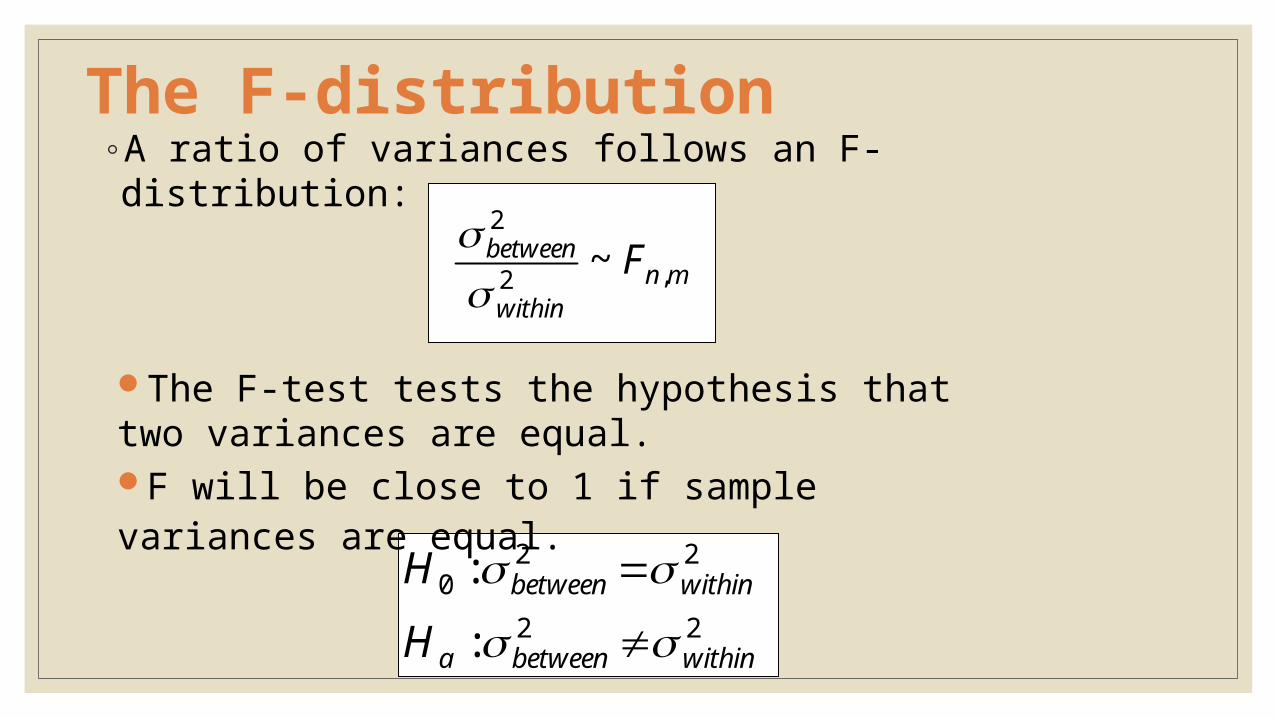
The F-distribution◦A ratio of variances follows an F-distribution:
22
220
:
:
withinbetweena
withinbetween
H
H
The F-test tests the hypothesis that two variances are equal. F will be close to 1 if sample variances are equal.
mnwithin
between F ,2
2
~

How to calculate ANOVA’s by hand…
Treatment 1 Treatment 2 Treatment 3 Treatment 4
y11 y21 y31 y41
y12 y22 y32 y42
y13 y23 y33 y43
y14 y24 y34 y44
y15 y25 y35 y45
y16 y26 y36 y46
y17 y27 y37 y47
y18 y28 y38 y48
y19 y29 y39 y49
y110 y210 y310 y410
n=10 obs./group
k=4 groups
The group means
10
10
11
1
jjy
y10
10
12
2
jjy
y10
10
13
3
jjy
y 10
10
14
4
jjy
y
The (within) group variances
110
)(10
1
211
j
j yy
110
)(10
1
222
j
j yy
110
)(10
1
233
j
j yy
110
)(10
1
244
j
j yy

Sum of Squares Within (SSW), or Sum of Squares Error (SSE)
The (within) group variances110
)(10
1
211
j
j yy
110
)(10
1
222
j
j yy
110
)(10
1
233
j
j yy
110
)(10
1
244
j
j yy
4
1
10
1
2)(i j
iij yy
+
10
1
211 )(
jj yy
10
1
222 )(
jj yy
10
3
233 )(
jj yy
10
1
244 )(
jj yy++
Sum of Squares Within (SSW) (or SSE, for chance error)

Sum of Squares Between (SSB), or Sum of Squares Regression (SSR)
Sum of Squares Between (SSB). Variability of the group means compared to the grand mean (the variability due to the treatment).
Overall mean of all 40 observations (“grand mean”)
40
4
1
10
1
i jijy
y
24
1
)(10
i
i yyx
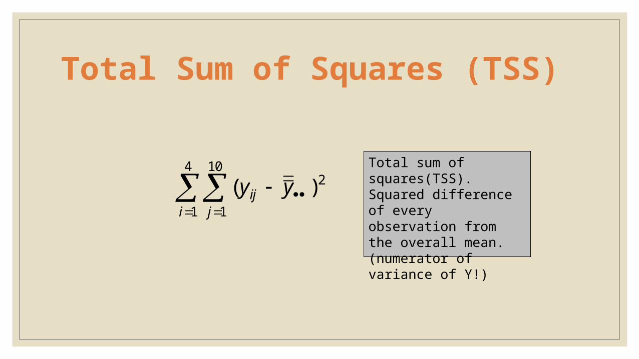
Total Sum of Squares (TSS)
Total sum of squares(TSS).Squared difference of every observation from the overall mean. (numerator of variance of Y!)
4
1
10
1
2)(i j
ij yy

Partitioning of Variance
4
1
10
1
2)(i j
iij yy
4
1
2)(i
i yy
4
1
10
1
2)(i j
ij yy=+
SSW + SSB = TSS
x10
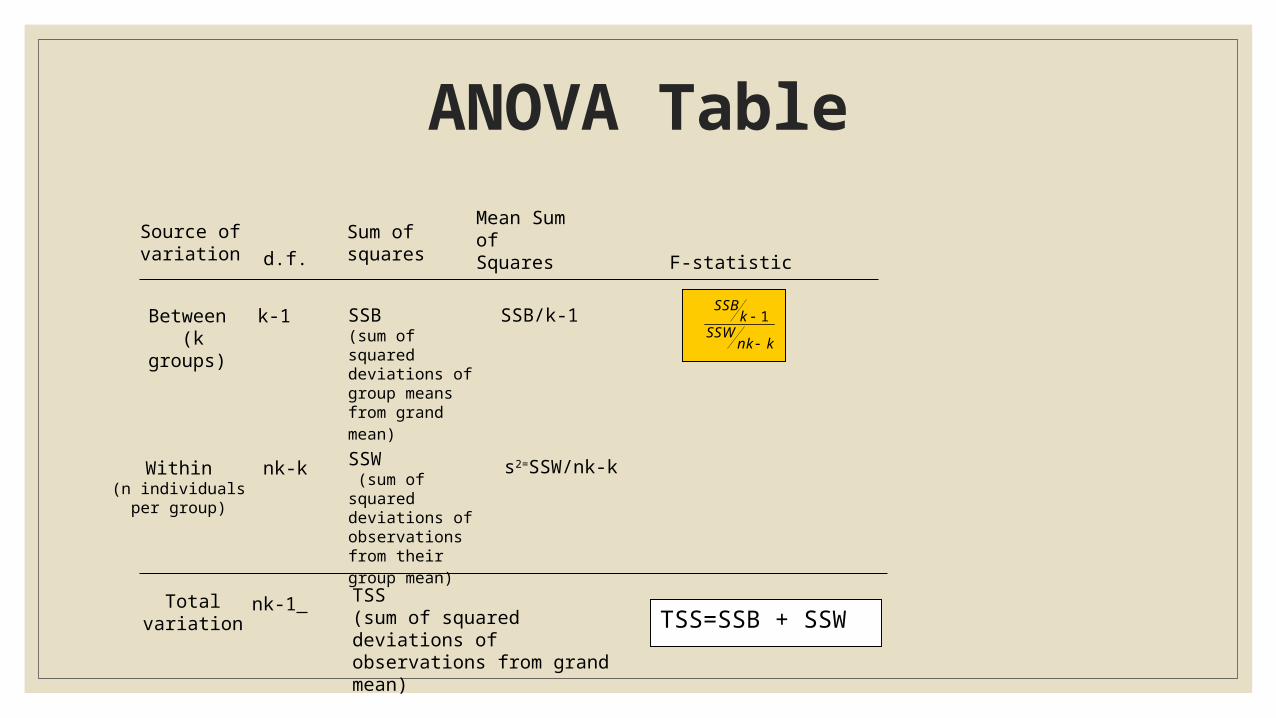
ANOVA Table
Between (k groups)
k-1 SSB(sum of squared deviations of group means from grand mean)
SSB/k-1
Total variation
nk-1 TSS(sum of squared deviations of observations from grand mean)
Source of variation
d.f.
Sum of squares
Mean Sum of Squares
F-statistic
Within(n individuals per
group)
nk-k SSW (sum of squared deviations of observations from their group mean)
s2=SSW/nk-k
knkSSW
kSSB
1
TSS=SSB + SSW

ANOVA=t-test
Between (2 groups)
1 SSB(squared differenc
e in means
multiplied by n)
Squared difference in means times n
Total variation
2n-1 TSS
Source of variation
d.f.
Sum of squares
Mean Sum of Squares F-statistic
Within 2n-2 SSW
equivalent to numerator of pooled variance
Pooled variance
222
2
222
2
)())(
()(
n
ppp
t
n
s
n
s
YX
s
YXn
222
2222
2
1
2
1
2
1
2
1
)()*2(
)2
*2)
2()
2(
2
*2)
2()
2((
)22
()22
(
))2
(())2
((
nnnnnn
nnnnnnnn
nnn
i
nnn
i
nnn
n
i
nnn
n
i
YXnYYXXn
YXXYYXYXn
XYn
YXn
YXYn
YXXnSSB
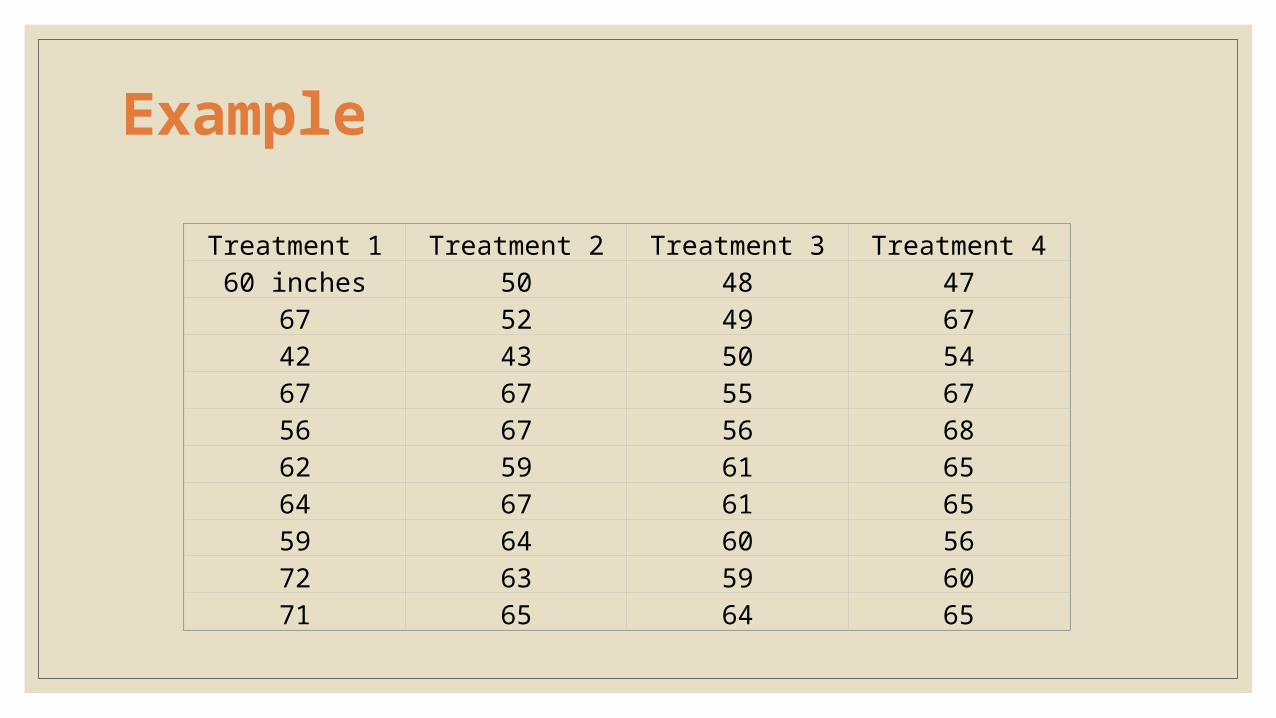
Example
Treatment 1 Treatment 2 Treatment 3 Treatment 4
60 inches 50 48 47
67 52 49 67
42 43 50 54
67 67 55 67
56 67 56 68
62 59 61 65
64 67 61 65
59 64 60 56
72 63 59 60
71 65 64 65

ExampleTreatment 1 Treatment 2 Treatment 3 Treatment 4
60 inches 50 48 47
67 52 49 67
42 43 50 54
67 67 55 67
56 67 56 68
62 59 61 65
64 67 61 65
59 64 60 56
72 63 59 60
71 65 64 65
Step 1) calculate the sum of squares between groups:
Mean for group 1 = 62.0
Mean for group 2 = 59.7
Mean for group 3 = 56.3
Mean for group 4 = 61.4
Grand mean= 59.85
SSB = [(62-59.85)2 + (59.7-59.85)2 + (56.3-59.85)2 + (61.4-59.85)2 ] xn per group= 19.65x10 = 196.5

ExampleTreatment 1 Treatment 2 Treatment 3 Treatment 4
60 inches 50 48 47
67 52 49 67
42 43 50 54
67 67 55 67
56 67 56 68
62 59 61 65
64 67 61 65
59 64 60 56
72 63 59 60
71 65 64 65
Step 2) calculate the sum of squares within groups:
(60-62) 2+(67-62) 2+ (42-62) 2+ (67-62) 2+ (56-62) 2+ (62-62) 2+ (64-62) 2+ (59-62) 2+ (72-62) 2+ (71-62) 2+ (50-59.7) 2+ (52-59.7)
2+ (43-59.7) 2+67-59.7) 2+ (67-59.7) 2+ (69-59.7) 2…+….(sum of 40 squared deviations) = 2060.6
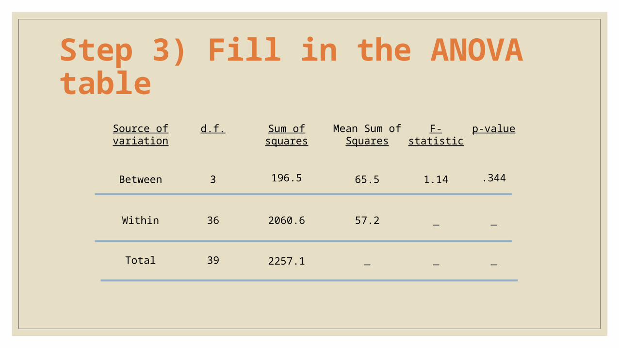
Step 3) Fill in the ANOVA table
3 196.5 65.5 1.14 .344
36 2060.6 57.2
Source of variation
d.f.
Sum of squares
Mean Sum of Squares
F-statistic
p-value
Between
Within
Total 39 2257.1

Step 3) Fill in the ANOVA table
3 196.5 65.5 1.14 .344
36 2060.6 57.2
Source of variation
d.f.
Sum of squares
Mean Sum of Squares
F-statistic
p-value
Between
Within
Total 39 2257.1
INTERPRETATION of ANOVA:
How much of the variance in height is explained by treatment group?
R2=“Coefficient of Determination” = SSB/TSS = 196.5/2275.1=9%

Coefficient of Determination
SST
SSB
SSESSB
SSBR
2
The amount of variation in the outcome variable (dependent variable) that is explained by the predictor (independent variable).

ANOVA example
S1a, n=25 S2b, n=25 S3c, n=25 P-valued
Calcium (mg) Mean 117.8 158.7 206.5 0.000SDe 62.4 70.5 86.2
Iron (mg) Mean 2.0 2.0 2.0 0.854
SD 0.6 0.6 0.6
Folate (μg) Mean 26.6 38.7 42.6 0.000
SD 13.1 14.5 15.1
Zinc (mg)Mean 1.9 1.5 1.3 0.055
SD 1.0 1.2 0.4a School 1 (most deprived; 40% subsidized lunches).b School 2 (medium deprived; <10% subsidized).c School 3 (least deprived; no subsidization, private school).d ANOVA; significant differences are highlighted in bold (P<0.05).
Mean micronutrient intake from the school lunch by school
FROM: Gould R, Russell J, Barker ME. School lunch menus and 11 to 12 year old children's food choice in three secondary schools in England-are the nutritional standards being met? Appetite. 2006 Jan;46(1):86-92.

Answer
Step 1) calculate the sum of squares between groups:
Mean for School 1 = 117.8
Mean for School 2 = 158.7
Mean for School 3 = 206.5
Grand mean: 161
SSB = [(117.8-161)2 + (158.7-161)2 + (206.5-161)2] x25 per group= 98,113

AnswerStep 2) calculate the sum of squares within groups:
S.D. for S1 = 62.4
S.D. for S2 = 70.5
S.D. for S3 = 86.2
Therefore, sum of squares within is:
(24)[ 62.42 + 70.5 2+ 86.22]=391,066
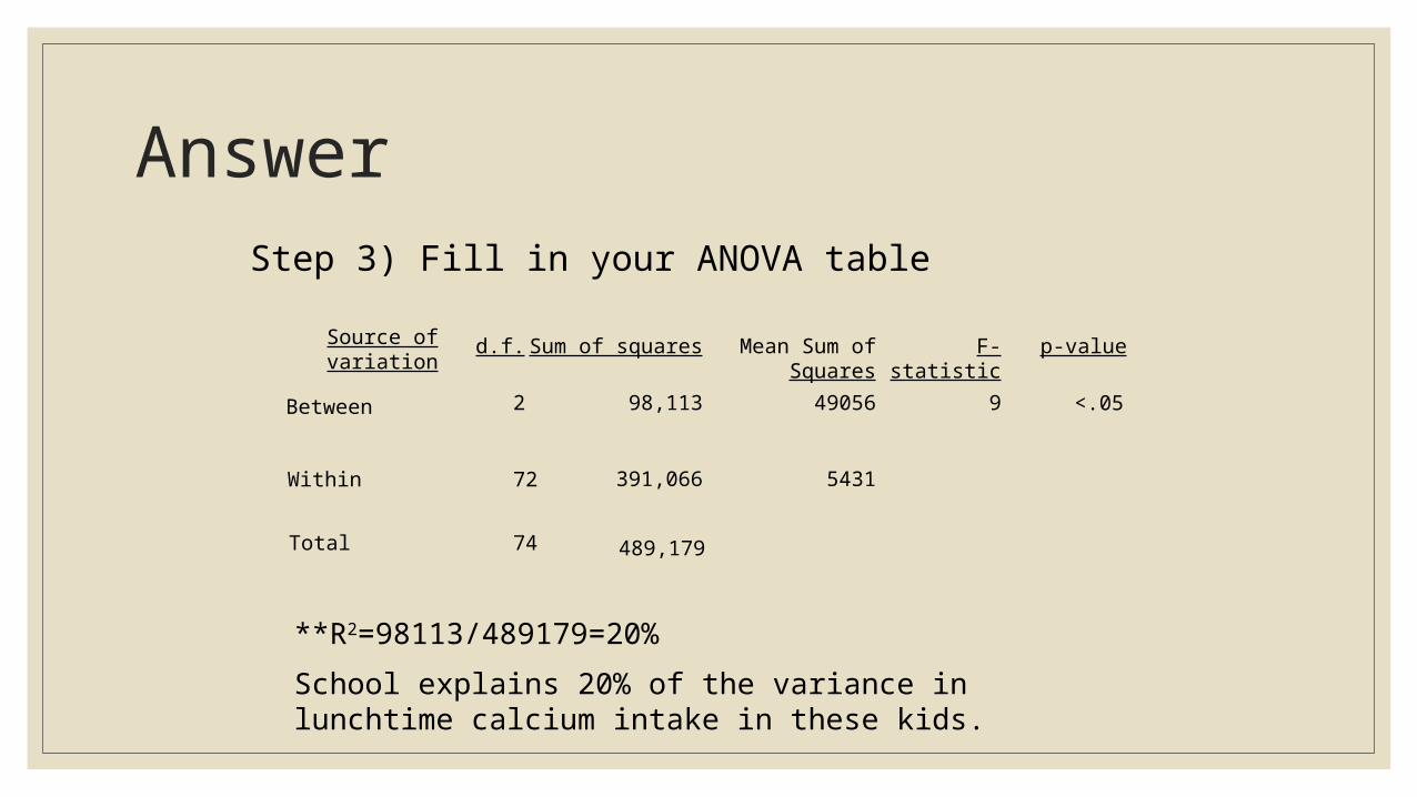
AnswerStep 3) Fill in your ANOVA table
Source of variation
d.f.
Sum of squares
Mean Sum of Squares
F-statistic
p-value
Between 2 98,113 49056 9 <.05
Within 72 391,066 5431
Total 74 489,179
**R2=98113/489179=20%
School explains 20% of the variance in lunchtime calcium intake in these kids.

ANOVA summary◦ A statistically significant ANOVA (F-test) only tells you that at least two of the
groups differ, but not which ones differ.
◦ Determining which groups differ (when it’s unclear) requires more sophisticated analyses to correct for the problem of multiple comparisons…

Correction for multiple comparisons
How to correct for multiple comparisons post-hoc…•Bonferroni correction (adjusts p by most conservative amount; assuming all tests independent, divide p by the number of tests)
•Tukey (adjusts p)•Scheffe (adjusts p)•Holm/Hochberg (gives p-cutoff beyond which not significant)
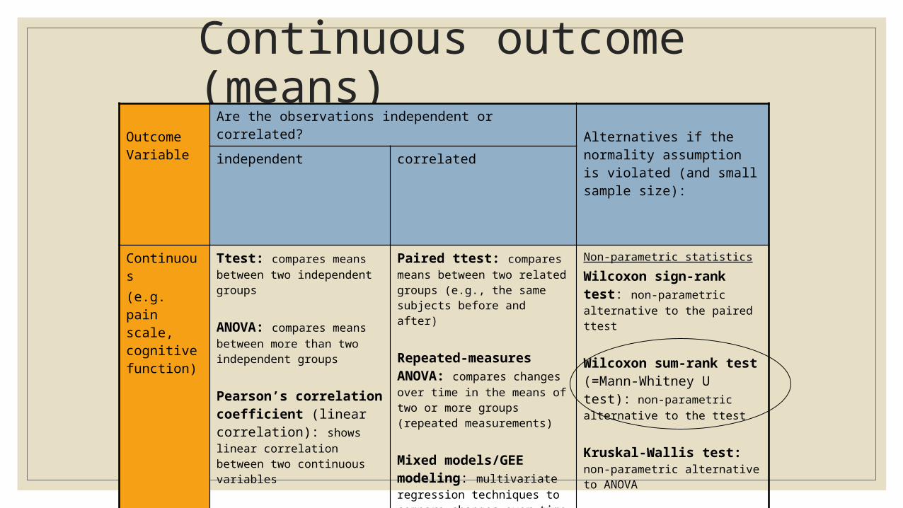
Continuous outcome (means)
Outcome Variable
Are the observations independent or correlated?Alternatives if the normality assumption is violated (and small sample size):
independent correlated
Continuous(e.g. pain scale, cognitive function)
Ttest: compares means between two independent groups
ANOVA: compares means between more than two independent groups
Pearson’s correlation coefficient (linear correlation): shows linear correlation between two continuous variables
Linear regression: multivariate regression technique used when the outcome is continuous; gives slopes
Paired ttest: compares means between two related groups (e.g., the same subjects before and after)
Repeated-measures ANOVA: compares changes over time in the means of two or more groups (repeated measurements)
Mixed models/GEE modeling: multivariate regression techniques to compare changes over time between two or more groups; gives rate of change over time
Non-parametric statistics
Wilcoxon sign-rank test: non-parametric alternative to the paired ttest
Wilcoxon sum-rank test (=Mann-Whitney U test): non-parametric alternative to the ttest
Kruskal-Wallis test: non-parametric alternative to ANOVA
Spearman rank correlation coefficient: non-parametric alternative to Pearson’s correlation coefficient

Binary or categorical outcomes (proportions)
Outcome Variable
Are the observations correlated? Alternative to the chi-square test if sparse cells:independent correlated
Binary or categorical(e.g. fracture, yes/no)
Chi-square test: compares proportions between two or more groups
Relative risks: odds ratios or risk ratios
Logistic regression: multivariate technique used when outcome is binary; gives multivariate-adjusted odds ratios
McNemar’s chi-square test: compares binary outcome between correlated groups (e.g., before and after)
Conditional logistic regression: multivariate regression technique for a binary outcome when groups are correlated (e.g., matched data)
GEE modeling: multivariate regression technique for a binary outcome when groups are correlated (e.g., repeated measures)
Fisher’s exact test: compares proportions between independent groups when there are sparse data (some cells <5).
McNemar’s exact test: compares proportions between correlated groups when there are sparse data (some cells <5).