Analysis of Urban Land Shortages: The Case of Korean Citieshompi.sogang.ac.kr/kyungkim/freeboard/papers/An... · Analysis of Urban Land Shortages: The Case of Korean Cities* Jae-Young

Ž .JOURNAL OF URBAN ECONOMICS 43, 362]384 1998ARTICLE NO. UE972051

Analysis of Urban Land Shortages: The Case ofKorean Cities*

Jae-Young Son

Department of Real Estate Studies, Kon-kuk Uni ersity, 93-1 Mo-jin Dong, Kwang-jinGu, Seoul, 143-701, Korea

and

Kyung-Hwan Kim

Department of Economics, Sogang Uni ersity, CPO Box 1142, Seoul, Korea

Received April 30, 1996; revised March 20, 1997

I. INTRODUCTION

Both natural constraints and government regulations on urban land usecan cause urban land shortages, and hence higher prices of urban land andhousing than otherwise. There have been attempts to investigate thedifferential effects of natural and contrived restrictions on land price. For

w xexample, Rose 10 found that natural constraints have a significantpositive impact on land value while monopoly zoning power makes asmaller contribution in explaining inter-city variations in urban land price.

w xOn the other hand, Pollakowski and Wachter 8 analyzed the impact ofland use controls measured by an index of restrictiveness of zoning andconfirmed that land use regulations raise the prices of housing anddeveloped land. To the best knowledge of the authors, however, none ofthe published empirical studies including the two cited above actuallymeasure the amount of shortage of urban land at the city level. Instead,land supply variables are employed together with demand variables such asincome and population size to determine their impact on land or housingprices.

This study seeks to fill the gap in the literature first by developing ameasure of the urban land shortagersurplus from an analysis of land price

*Comments by Jan Brueckner and two anonymous referees on an earlier draft aregratefully acknowledged.

362

0094-1190r98 $25.00Copyright Q 1998 by Academic PressAll rights of reproduction in any form reserved.

URBAN LAND SHORTAGES IN KOREA 363

gradients within the framework of the standard monocentric urban model.This is done in Section II. Then the model is applied to measure themagnitude of urban land shortages in Korean cities. Korea has a system ofstringent controls on the conversion of land use from rural to urban as wellas exhibiting a remarkable pace of economic growth and urbanization. Amajor consequence of the artificial scarcity of developable land caused bygovernment regulation and rapidly increasing demand for urban land isthat housing is unaffordable to a large part of the country’s urban

w xpopulation 2, 4 . In order to test whether urban land use controls aremainly responsible for urban land shortages, extensive data on land valueon 300,000 plots in 171 cities and counties in Korea were used to compute

Ž .the amount of land shortages Section III and to relate the estimatedŽ .shortage figures to natural and regulatory constraints Section IV . Section

V concludes the paper with a summary of major findings and policyimplications.

II. CONCEPTUAL FRAMEWORK FOR MEASURINGURBAN LAND SHORTAGE OR SURPLUS

1. Allocation of Land between Urban and Rural Use in a Monocentric CityModel

Our approach to measure shortagersurplus of urban land in a givencity1 builds on the standard monocentric city model with a predetermined

Ž .urban center CBD on a featureless plane with no topographical andregulatory constraints.2 The standard model recognizes two competingtypes of land use: urban land used for housing, industrial, commercial, andinfrastructure; and rural land devoted to agricultural, forestal, and pastoraluses. The opportunity cost of urban land, i.e., the rural land price, isassumed to be zero or a fixed constant in simple versions of the model.However, the price of rural land may vary with distance from the centerbecause proximity to the center benefits certain kinds of non-urbaneconomic activities. In addition, the cost associated with converting ruralland into urban use and installing urban infrastructure must be added tothe opportunity cost of urban land.

1In this paper, the term ‘‘city’’ refers to an area with an urban center surrounded by ruralhinterland. When it is used in contrast to the ‘‘county,’’ however, the city is a statutory entitywith a legal jurisdiction. It should be noted that, in Korea, the city and the county areseparate administrative units with mutually exclusive jurisdictions. An urbanized area within acounty can gain the status of a city when its population reaches 50,000. The city and thecounty belong to the province, but the six largest cities have the same legal status as aprovince.

2 w xRefer to 1 for an excellent exposition of the model.

SON AND KIM364

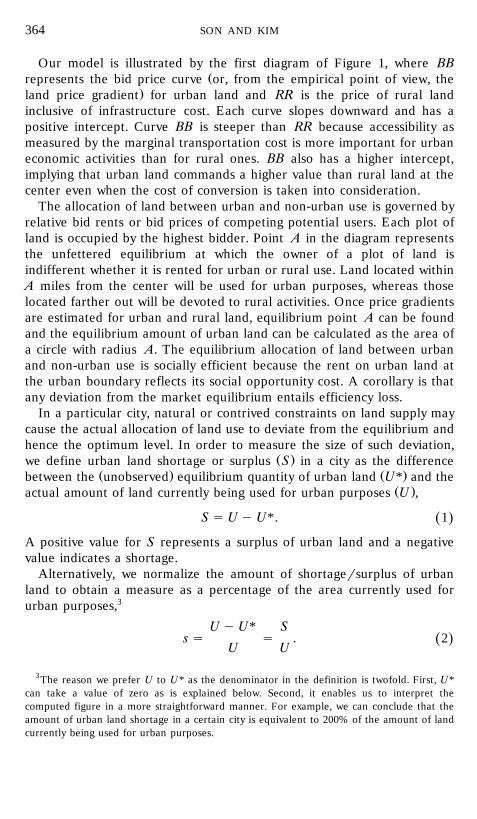
Our model is illustrated by the first diagram of Figure 1, where BBŽrepresents the bid price curve or, from the empirical point of view, the

.land price gradient for urban land and RR is the price of rural landinclusive of infrastructure cost. Each curve slopes downward and has apositive intercept. Curve BB is steeper than RR because accessibility asmeasured by the marginal transportation cost is more important for urbaneconomic activities than for rural ones. BB also has a higher intercept,implying that urban land commands a higher value than rural land at thecenter even when the cost of conversion is taken into consideration.

The allocation of land between urban and non-urban use is governed byrelative bid rents or bid prices of competing potential users. Each plot ofland is occupied by the highest bidder. Point A in the diagram representsthe unfettered equilibrium at which the owner of a plot of land isindifferent whether it is rented for urban or rural use. Land located withinA miles from the center will be used for urban purposes, whereas thoselocated farther out will be devoted to rural activities. Once price gradientsare estimated for urban and rural land, equilibrium point A can be foundand the equilibrium amount of urban land can be calculated as the area ofa circle with radius A. The equilibrium allocation of land between urbanand non-urban use is socially efficient because the rent on urban land atthe urban boundary reflects its social opportunity cost. A corollary is thatany deviation from the market equilibrium entails efficiency loss.

In a particular city, natural or contrived constraints on land supply maycause the actual allocation of land use to deviate from the equilibrium andhence the optimum level. In order to measure the size of such deviation,

Ž .we define urban land shortage or surplus S in a city as the differenceŽ . Ž .between the unobserved equilibrium quantity of urban land U* and the

Ž .actual amount of land currently being used for urban purposes U ,

S s U y U*. 1Ž .A positive value for S represents a surplus of urban land and a negativevalue indicates a shortage.

Alternatively, we normalize the amount of shortagersurplus of urbanland to obtain a measure as a percentage of the area currently used forurban purposes,3

U y U* Ss s s . 2Ž .

U U

3The reason we prefer U to U* as the denominator in the definition is twofold. First, U*can take a value of zero as is explained below. Second, it enables us to interpret thecomputed figure in a more straightforward manner. For example, we can conclude that theamount of urban land shortage in a certain city is equivalent to 200% of the amount of landcurrently being used for urban purposes.


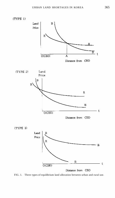
FIG. 1. Three types of equilibrium land allocation between urban and rural use.

SON AND KIM366

Although published data on U are available at the city level, U* must becomputed using land price data. Calculation of U* is conceptually straight-forward in a standard monocentric model with no land use restrictions, butcritical assumptions of the model may not be satisfied in real world cities.Therefore, we devise a method to deal with the natural and contrivedconstraints which cause real cities to exhibit a spatial structure differentfrom that derived in the standard model. Since our approach cannotaccommodate all violations of the standard assumptions, we will identifyconditions under which our method is likely or not likely to producereliable estimates of land shortages.

2. Discussion of the Assumptions

Topography

The standard monocentric model assumes that the city is situated in afeatureless plane with no topographical constraints. In a real world city,there may be bodies of water or mountains. To the extent these topograph-ical constraints are effectively overcome by bridges, tunnels, and othertransportation facilities, easy accessibility to the CBD justifies the assump-tion of a featureless plain. However, there must be cities where topographyhinders access to the CBD and the estimated land price gradients aredistorted.4 A region consisting of several islands, each having its ownpopulation center is one example, and an urban area developed linearlyalong a transportation corridor is another. In such cities, the slope of theurban land price gradient will be very small, resulting in an overestimationof the optimal urban land area. Although our data do not allow us todetermine a priori whether topographical constraints cause distorted re-sults, a topographical problem is suspected if the slope of land pricegradients is unusually small.

Another potential problem arising from irregular topography is that theestimated land price function could be misinterpreted in calculating theshortage of urban land. Take the case of a city developed around awaterfront CBD. If one assumes that the city is circular in shape, theequilibrium quantity of urban land U* would be calculated as p A2, but thecorrect figure is one-half of the estimate. This problem can arise wheneverthe overall shape of the city is much different from a circle or the CBD islocated in a far corner of the city. To deal with such situations, we define atopographical adjustment factor and apply it when computing the equilib-rium quantity of urban land.

4 w xRose 10 defines the concept of a finite land supply as a weighted sum of units of landspace available in a city, taking topographical constraints into consideration.


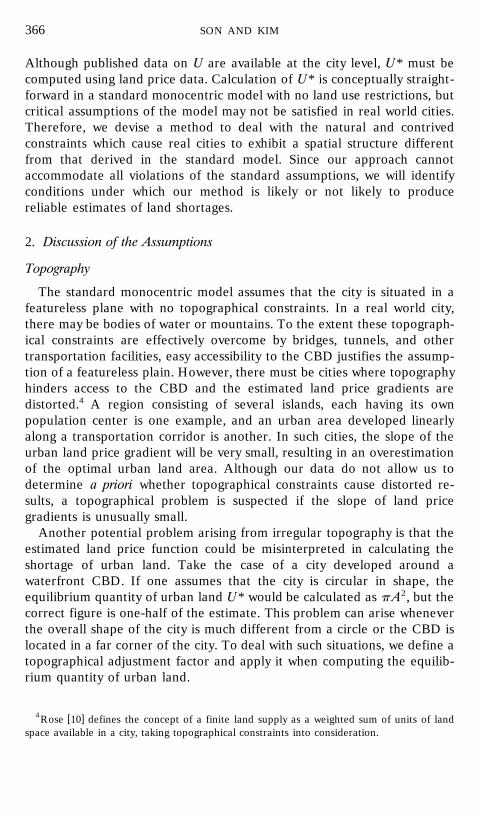
FIG. 2. Equilibrium land use in a city with subcenters.

MonocentricityThe assumption that all economic activities take place at a single

predetermined center is highly restrictive.5 Some cities may have well-developed subcenters which entail more than one peak of urban land pricegradient. Figure 2 illustrates a city with a set of subcenters located along aband at Y miles from the center. Curve KLMN is the true profile of urbanland price, whereas Pr represents a fixed price of non-urban land. Inequilibrium, plots between O and A and those between point B and pointC will be used for urban purposes, while plots located between A and Band those beyond point C will be used for non-urban activities. If one fitsa monotonically declining urban land price schedule ignoring the existenceof subcenters, a line like B9B9 will be estimated, and the equilibriumquantity of urban land will be calculated incorrectly.6

This problem can be avoided if one has accurate information on thelocation of subcenters as well as the CBD. Since our data set does nothave such information, there is room for inaccuracy in our estimate ofurban land shortage for some cities. This problem can be detected byclosely examining the estimation results of land price gradients.

Regulatory Constraints and Open City AssumptionThe most critical assumption in our analysis is that of a small open city.

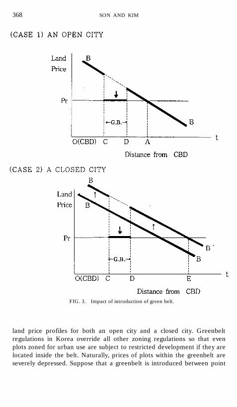
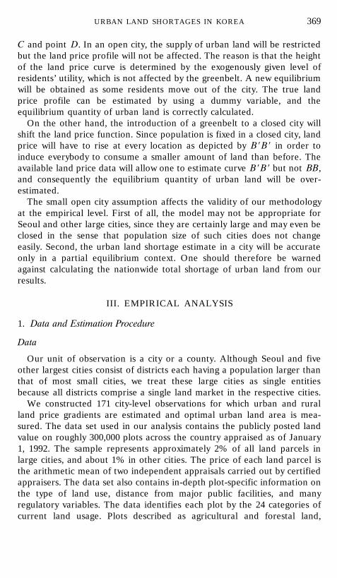
Only under this assumption is it possible to estimate correctly the optimalurban land area from the available data. This point is illustrated in Figure3. The two diagrams display the impact of greenbelt regulations on the

5 w x w xSee 9 for criticism of the assumption and 11 for a model that deals with this issue.6 Ž .The nature of the problem arising from subcenter s is similar to the problem of

topographical barriers discussed earlier. Two urban areas separated by a body of water butwithout a transportation link such as a bridge can be seen as two subcenters.

SON AND KIM368

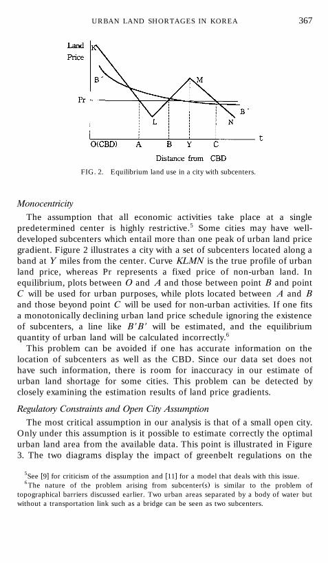
FIG. 3. Impact of introduction of green belt.

land price profiles for both an open city and a closed city. Greenbeltregulations in Korea override all other zoning regulations so that evenplots zoned for urban use are subject to restricted development if they arelocated inside the belt. Naturally, prices of plots within the greenbelt areseverely depressed. Suppose that a greenbelt is introduced between point


C and point D. In an open city, the supply of urban land will be restrictedbut the land price profile will not be affected. The reason is that the heightof the land price curve is determined by the exogenously given level ofresidents’ utility, which is not affected by the greenbelt. A new equilibriumwill be obtained as some residents move out of the city. The true landprice profile can be estimated by using a dummy variable, and theequilibrium quantity of urban land is correctly calculated.

On the other hand, the introduction of a greenbelt to a closed city willshift the land price function. Since population is fixed in a closed city, landprice will have to rise at every location as depicted by B9B9 in order toinduce everybody to consume a smaller amount of land than before. Theavailable land price data will allow one to estimate curve B9B9 but not BB,and consequently the equilibrium quantity of urban land will be over-estimated.

The small open city assumption affects the validity of our methodologyat the empirical level. First of all, the model may not be appropriate forSeoul and other large cities, since they are certainly large and may even beclosed in the sense that population size of such cities does not changeeasily. Second, the urban land shortage estimate in a city will be accurateonly in a partial equilibrium context. One should therefore be warnedagainst calculating the nationwide total shortage of urban land from ourresults.

III. EMPIRICAL ANALYSIS

1. Data and Estimation Procedure

Data

Our unit of observation is a city or a county. Although Seoul and fiveother largest cities consist of districts each having a population larger thanthat of most small cities, we treat these large cities as single entitiesbecause all districts comprise a single land market in the respective cities.

We constructed 171 city-level observations for which urban and ruralland price gradients are estimated and optimal urban land area is mea-sured. The data set used in our analysis contains the publicly posted landvalue on roughly 300,000 plots across the country appraised as of January1, 1992. The sample represents approximately 2% of all land parcels inlarge cities, and about 1% in other cities. The price of each land parcel isthe arithmetic mean of two independent appraisals carried out by certifiedappraisers. The data set also contains in-depth plot-specific information onthe type of land use, distance from major public facilities, and manyregulatory variables. The data identifies each plot by the 24 categories ofcurrent land usage. Plots described as agricultural and forestal land,

SON AND KIM370

pasture, and bodies of water are classified as rural, and the rest areclassified as urban. In addition to residential, commercial, and industrialbuilding sites, urban land includes such public property as roads, railways,parks, and plots for ‘‘miscellaneous use.’’ Since the last category of plotsmay be used for either urban or rural purposes, we would be safer with aconclusion that urban land is in short supply.

Land Price Gradients

We estimate land price gradients like BB and RR in Figure 1 by fittingseparate negative exponential land price gradients for urban and ruralplots7:

Log Pu s a q a t q a D q a D ? t q u 3Ž .0 1 2 3

Log Pr q C s b q b t q b D q b D ? t q ¨ , 4Ž . Ž .0 1 2 3

where Pu and Pr refer to the price of a plot measuring one square meterin urban and rural use, respectively. C is the cost of developing one squaremeter of non-urban land into urban land, and t represents the airlinedistance from the center of the city defined as the site of the city hall orthe county administrative office. u and ¨ are error terms. The dummyvariable D intends to capture the effect of the greenbelt in which landdevelopment is virtually prohibited. The variable takes a value of 1 if a plotis located inside the greenbelt area and zero otherwise. As for the landdevelopment cost C, we borrowed the figure of 93,000 won per square

w xmeter from Chung-Ho Kim 3 , who computed it from the cost data on thesites developed and serviced by the Korea Land Development Corpora-tion, the dominant public sector developer. We assume that the develop-ment cost does not vary from city to city.

Calculation of the Equilibrium Amount of Urban Land

Since a land price gradient is represented by two critical parameters,slope and intercept, there are four possible types of allocation of landbetween urban and rural use. However, only three types were obtained inour empirical analysis as depicted in Figure 1. For each type, the equilib-rium urban land area is calculated as follows.

Type 1. Type 1 represents the most realistic outcome in that the urbanland price curve has both a steeper slope and a greater intercept than its

Ž < < < < .rural counterpart a ) b and a ) b . We set the greenbelt dummy1 1 0 0variable equal to zero to find the unfettered equilibrium. Therefore,

7 w xThis may lead to selectivity bias. See 7 for an example of addressing the problem. Alsow xrefer to 6 for a discussion of limitations of the negative exponential functional form.


distance from the center to the equilibrium urban boundary A is deter-mined by

A s a y b r b y a 5Ž . Ž . Ž .0 0 1 1

Several adjustments are required since real world cities may not satisfy thestandard assumptions of the model. In order to deal with cases such ascities with waterfront CBD, we first select the 2% of plots farthest from

Ž .the center, and calculate the average distance L of those plots from thecenter. Then we compute the ratio r between the area of a circle withradius L and the actual land area within the legal boundary of the city, V:

p L2

r s . 6Ž .V

If a city is circular in shape with its CBD located close to the center of thecircle and there are enough observations near the boundary, then r willtake a value close to 1. On the other hand, non-circular cities or citieswhose centers are not at the center of the circle are likely to have an rwhich is greater than 1. Although it is conceptually impossible for r to beless than 1, several such cases were found in our sample due to insufficientobservations near the boundary. In order to eliminate them, we define atopographical adjustment factor as

� 4r* s MAX 1, r . 7Ž .

This leads to the equilibrium amount of urban land of a city which is equalto p A2rr*, but it must be adjusted to ensure that the computed value isless than the total land area V within its legal boundary,

U* s MIN p A2rr* , V . 8Ž .� 4Ž .

Type 2. Type 2 refers to the case in which rural land price plusŽ < < < <conversion cost exceeds urban land price in all locations a ) b and1 1

. Ž .a - b . Since BB and RR intersect to the left of the origin A - 0 , we0 0set the equilibrium amount of urban land U* equal to zero. We interpretType 2 as the situation in which no land should be devoted to urban usebecause of the high opportunity cost of urban land. All Type 2 cities have a

Ž .surplus of urban land S ) 0 and s ) 0 .

Type 3. Type 3 is the case where BB lies above RR at all locations sothat more than the whole land area of the city should be used for urban

Ž < < < < .purposes in equilibrium a - b and a ) b . All Type 3 cities have a1 1 0 0Ž .shortage of urban land S - 0 and s - 0 . Although this type can arise in

highly urbanized cities where the development pressure overflows the cityboundary, it can also occur because the city in question does not satisfy the

SON AND KIM372

assumptions of the model such as monocentricity or featureless topogra-phy. We set U* equal to V.

2. Estimation Results

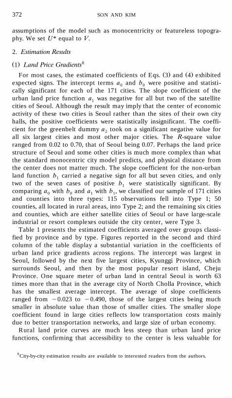
Ž . 81 Land Price GradientsŽ . Ž .For most cases, the estimated coefficients of Eqs. 3 and 4 exhibited

expected signs. The intercept terms a and b were positive and statisti-0 0cally significant for each of the 171 cities. The slope coefficient of theurban land price function a was negative for all but two of the satellite1cities of Seoul. Although the result may imply that the center of economicactivity of these two cities is Seoul rather than the sites of their own cityhalls, the positive coefficients were statistically insignificant. The coeffi-cient for the greenbelt dummy a took on a significant negative value for2all six largest cities and most other major cities. The R-square valueranged from 0.02 to 0.70, that of Seoul being 0.07. Perhaps the land pricestructure of Seoul and some other cities is much more complex than whatthe standard monocentric city model predicts, and physical distance fromthe center does not matter much. The slope coefficient for the non-urbanland function b carried a negative sign for all but seven cities, and only1two of the seven cases of positive b were statistically significant. By1comparing a with b and a with b , we classified our sample of 171 cities0 0 1 1and counties into three types: 115 observations fell into Type 1; 50counties, all located in rural areas, into Type 2; and the remaining six citiesand counties, which are either satellite cities of Seoul or have large-scaleindustrial or resort complexes outside the city center, were Type 3.

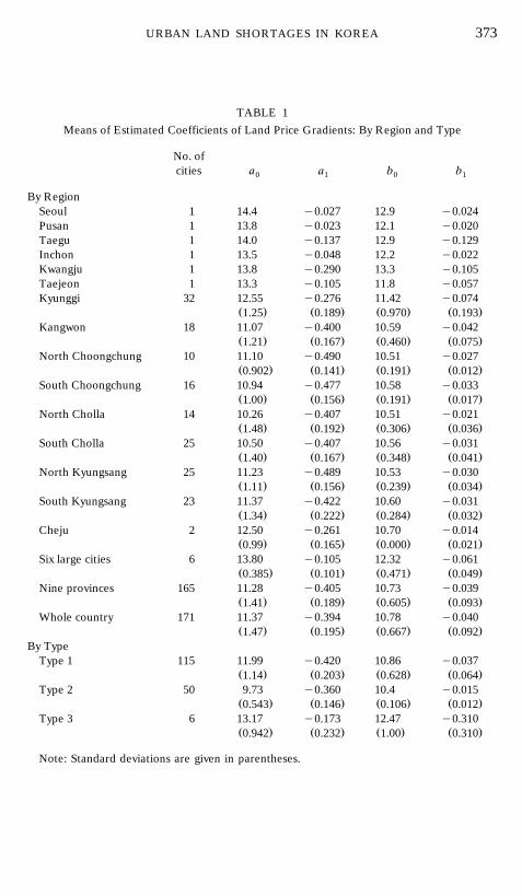
Table 1 presents the estimated coefficients averaged over groups classi-fied by province and by type. Figures reported in the second and thirdcolumn of the table display a substantial variation in the coefficients ofurban land price gradients across regions. The intercept was largest inSeoul, followed by the next five largest cities, Kyunggi Province, whichsurrounds Seoul, and then by the most popular resort island, ChejuProvince. One square meter of urban land in central Seoul is worth 63times more than that in the average city of North Cholla Province, whichhas the smallest average intercept. The average of slope coefficientsranged from y0.023 to y0.490, those of the largest cities being muchsmaller in absolute value than those of smaller cities. The smaller slopecoefficient found in large cities reflects low transportation costs mainlydue to better transportation networks, and large size of urban economy.

Rural land price curves are much less steep than urban land pricefunctions, confirming that accessibility to the center is less valuable for

8City-by-city estimation results are available to interested readers from the authors.


TABLE 1Means of Estimated Coefficients of Land Price Gradients: By Region and Type

No. ofcities a a b b0 1 0 1

By RegionSeoul 1 14.4 y0.027 12.9 y0.024Pusan 1 13.8 y0.023 12.1 y0.020Taegu 1 14.0 y0.137 12.9 y0.129Inchon 1 13.5 y0.048 12.2 y0.022Kwangju 1 13.8 y0.290 13.3 y0.105Taejeon 1 13.3 y0.105 11.8 y0.057Kyunggi 32 12.55 y0.276 11.42 y0.074

Ž . Ž . Ž . Ž .1.25 0.189 0.970 0.193Kangwon 18 11.07 y0.400 10.59 y0.042

Ž . Ž . Ž . Ž .1.21 0.167 0.460 0.075North Choongchung 10 11.10 y0.490 10.51 y0.027

Ž . Ž . Ž . Ž .0.902 0.141 0.191 0.012South Choongchung 16 10.94 y0.477 10.58 y0.033

Ž . Ž . Ž . Ž .1.00 0.156 0.191 0.017North Cholla 14 10.26 y0.407 10.51 y0.021

Ž . Ž . Ž . Ž .1.48 0.192 0.306 0.036South Cholla 25 10.50 y0.407 10.56 y0.031

Ž . Ž . Ž . Ž .1.40 0.167 0.348 0.041North Kyungsang 25 11.23 y0.489 10.53 y0.030

Ž . Ž . Ž . Ž .1.11 0.156 0.239 0.034South Kyungsang 23 11.37 y0.422 10.60 y0.031

Ž . Ž . Ž . Ž .1.34 0.222 0.284 0.032Cheju 2 12.50 y0.261 10.70 y0.014

Ž . Ž . Ž . Ž .0.99 0.165 0.000 0.021Six large cities 6 13.80 y0.105 12.32 y0.061

Ž . Ž . Ž . Ž .0.385 0.101 0.471 0.049Nine provinces 165 11.28 y0.405 10.73 y0.039

Ž . Ž . Ž . Ž .1.41 0.189 0.605 0.093Whole country 171 11.37 y0.394 10.78 y0.040

Ž . Ž . Ž . Ž .1.47 0.195 0.667 0.092By Type

Type 1 115 11.99 y0.420 10.86 y0.037Ž . Ž . Ž . Ž .1.14 0.203 0.628 0.064

Type 2 50 9.73 y0.360 10.4 y0.015Ž . Ž . Ž . Ž .0.543 0.146 0.106 0.012

Type 3 6 13.17 y0.173 12.47 y0.310Ž . Ž . Ž . Ž .0.942 0.232 1.00 0.310

Note: Standard deviations are given in parentheses.

SON AND KIM374

rural activities than for urban ones. Inter-regional variation of interceptsand slope coefficients is small compared to that of urban land pricefunctions. As was true of urban land price functions, six large cities andKyunggi Province have higher intercepts than other provinces, indicatingthat the prospect of land use change is already reflected in the price ofrural land. One should note, however, that rural land hypothetically at thecenter of Seoul would be only 10.9 times as expensive as its counterpart inNorth Cholla Province compared with the ratio of 63 reported above forurban land prices.

Among the six largest cities, the slope of the non-urban land pricecurves is quite small for Seoul, Pusan, and Inchon, while the slope for theremaining three is relatively large. The magnitude of the average slopesfor the provinces falls in-between. We do not have a convincing explana-tion for the large variation of slope coefficients among the six large cities,but it is interesting to note that the difference in the average slopecoefficients between urban and non-urban functions is much larger in theprovinces than in the six large cities. This implies that the smaller cities inthese provinces have an economy which requires only small land areas.Finally, among the provinces, with a possible exception of Cheju Province,the average of intercepts of both urban and rural land price gradientsvaries little, and the standard deviation of intercepts is only about one-tenth

Žof the average. This indicates that the price of urban land and hypotheti-.cal rural land as well at the center is similar among small cities across the

country. It also implies that the size of urban economy in small cities maybe more or less uniform across the country.

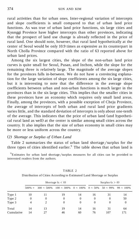
Ž .2 Shortage or Surplus of Urban LandTable 2 summarizes the status of urban land shortagersurplus for the

three types of cities identified earlier.9 The table shows that urban land is9 Estimates for urban land shortagersurplus measures for all cities can be provided to

interested readers from the authors.

TABLE 2Distribution of Cities According to Estimated Land Shortage or Surplus

Ž . Ž .Shortage s - 0 Surplus s ) 0

500%q 300 ; 500% 100 ; 300% 0 ; 100% 0 ; 50% 50 ; 99% 99 ; 100%

Type 1 10 11 19 14 16 31 14Type 2 0 0 0 0 0 0 50Type 3 4 2 0 0 0 0 0

Total 14 13 19 14 16 31 64Cumulative 14 27 46 60 76 107 171


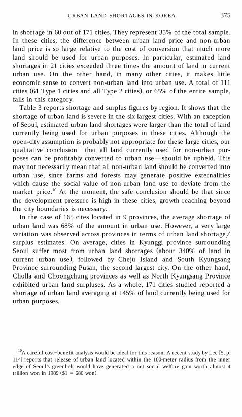
in shortage in 60 out of 171 cities. They represent 35% of the total sample.In these cities, the difference between urban land price and non-urbanland price is so large relative to the cost of conversion that much moreland should be used for urban purposes. In particular, estimated landshortages in 21 cities exceeded three times the amount of land in currenturban use. On the other hand, in many other cities, it makes littleeconomic sense to convert non-urban land into urban use. A total of 111

Ž .cities 61 Type 1 cities and all Type 2 cities , or 65% of the entire sample,falls in this category.

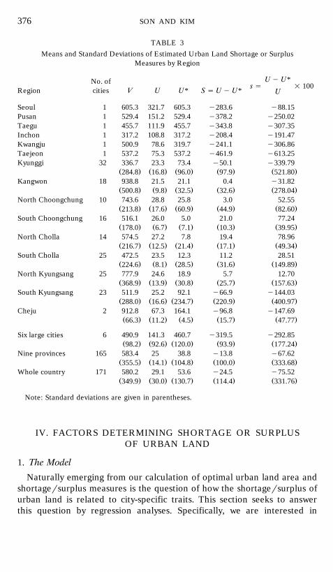
Table 3 reports shortage and surplus figures by region. It shows that theshortage of urban land is severe in the six largest cities. With an exceptionof Seoul, estimated urban land shortages were larger than the total of landcurrently being used for urban purposes in these cities. Although theopen-city assumption is probably not appropriate for these large cities, ourqualitative conclusion}that all land currently used for non-urban pur-poses can be profitably converted to urban use}should be upheld. Thismay not necessarily mean that all non-urban land should be converted intourban use, since farms and forests may generate positive externalitieswhich cause the social value of non-urban land use to deviate from themarket price.10 At the moment, the safe conclusion should be that sincethe development pressure is high in these cities, growth reaching beyondthe city boundaries is necessary.

In the case of 165 cites located in 9 provinces, the average shortage ofurban land was 68% of the amount in urban use. However, a very largevariation was observed across provinces in terms of urban land shortagersurplus estimates. On average, cities in Kyunggi province surrounding

ŽSeoul suffer most from urban land shortages about 340% of land in.current urban use , followed by Cheju Island and South Kyungsang

Province surrounding Pusan, the second largest city. On the other hand,Cholla and Choongchung provinces as well as North Kyungsang Provinceexhibited urban land surpluses. As a whole, 171 cities studied reported ashortage of urban land averaging at 145% of land currently being used forurban purposes.

10 wA careful cost]benefit analysis would be ideal for this reason. A recent study by Lee 5, p.x114 reports that release of urban land located within the 100-meter radius from the inner

edge of Seoul’s greenbelt would have generated a net social welfare gain worth almost 4Ž .trillion won in 1989 $1 s 680 won .

SON AND KIM376

TABLE 3Means and Standard Deviations of Estimated Urban Land Shortage or Surplus

Measures by Region

U y U*No. ofs s = 100

Region cities V U U* S s U y U* U

Seoul 1 605.3 321.7 605.3 y283.6 y88.15Pusan 1 529.4 151.2 529.4 y378.2 y250.02Taegu 1 455.7 111.9 455.7 y343.8 y307.35Inchon 1 317.2 108.8 317.2 y208.4 y191.47Kwangju 1 500.9 78.6 319.7 y241.1 y306.86Taejeon 1 537.2 75.3 537.2 y461.9 y613.25Kyunggi 32 336.7 23.3 73.4 y50.1 y339.79

Ž . Ž . Ž . Ž . Ž .284.8 16.8 96.0 97.9 521.80Kangwon 18 938.8 21.5 21.1 0.4 y31.82

Ž . Ž . Ž . Ž . Ž .500.8 9.8 32.5 32.6 278.04North Choongchung 10 743.6 28.8 25.8 3.0 52.55

Ž . Ž . Ž . Ž . Ž .213.8 17.6 60.9 44.9 82.60South Choongchung 16 516.1 26.0 5.0 21.0 77.24

Ž . Ž . Ž . Ž . Ž .178.0 6.7 7.1 10.3 39.95North Cholla 14 574.5 27.2 7.8 19.4 78.96

Ž . Ž . Ž . Ž . Ž .216.7 12.5 21.4 17.1 49.34South Cholla 25 472.5 23.5 12.3 11.2 28.51

Ž . Ž . Ž . Ž . Ž .224.6 8.1 28.5 31.6 149.89North Kyungsang 25 777.9 24.6 18.9 5.7 12.70

Ž . Ž . Ž . Ž . Ž .368.9 13.9 30.8 25.7 157.63South Kyungsang 23 511.9 25.2 92.1 y66.9 y144.03

Ž . Ž . Ž . Ž . Ž .288.0 16.6 234.7 220.9 400.97Cheju 2 912.8 67.3 164.1 y96.8 y147.69

Ž . Ž . Ž . Ž . Ž .66.3 11.2 4.5 15.7 47.77

Six large cities 6 490.9 141.3 460.7 y319.5 y292.85Ž . Ž . Ž . Ž . Ž .98.2 92.6 120.0 93.9 177.24

Nine provinces 165 583.4 25 38.8 y13.8 y67.62Ž . Ž . Ž . Ž . Ž .355.5 14.1 104.8 100.0 333.68

Whole country 171 580.2 29.1 53.6 y24.5 y75.52Ž . Ž . Ž . Ž . Ž .349.9 30.0 130.7 114.4 331.76

Note: Standard deviations are given in parentheses.

IV. FACTORS DETERMINING SHORTAGE OR SURPLUSOF URBAN LAND

1. The Model

Naturally emerging from our calculation of optimal urban land area andshortagersurplus measures is the question of how the shortagersurplus ofurban land is related to city-specific traits. This section seeks to answerthis question by regression analyses. Specifically, we are interested in


testing the hypothesis that urban land shortage in Korea results fromgovernment regulations which restrict land development and supply. Thiscan be done by regressing a measure of urban land shortage againstexplanatory variables representing natural and regulatory constraints andother variables. The hypothesis can be justified if the regulatory variablescarry a significant sign.

The small-and-open city assumption which justifies our measurement ofurban land shortagersurplus also determines the structure of the regres-sion equation. Under this assumption, the position of the bid price func-tion is determined by the economic conditions of the system of cities towhich an individual city belongs, rather than by city specific demandfactors. Therefore, the magnitude of urban land shortagersurplus of anindividual city is explained only by supply side factors such as natural andcontrived restrictions on land use and development. If the assumptionfails, both demand and supply factors would affect the land shortagersurplus measure, so that the measure developed in this study may not becorrect. Whether a city is ‘‘open’’ or ‘‘closed’’ is an empirical issue, andclear-cut classification is not always possible. We thus present both sets ofregression results: one without demand variables and the other with them.

We have also noted that estimated land shortagersurplus figures for thesix largest cities, Type 3 cities, and those in the Capital region may sufferfrom measurement problems, in part because they are likely to be closedcities. In order to secure robust results from our regression analysis, weform three different samples by successively eliminating such cities. Sam-ple 1 is composed of all 171 cities, but Sample 2 takes out the six largestcities and Type 3 cities. Sample 3 further omits all cities in the Capitalregion. By estimating separate regressions on these three samples andcomparing the results, we will be able to obtain stable conclusions andfurther insights as to how characteristics of the city affect the shortagersurplus measure.

2. VariablesŽEach regression equation has the shortagersurplus measure s in per-

.centage units as the dependent variable. An increase in s means thaturban land surplus increases or its shortage decreases, and vice versa.Explanatory variables can be grouped as follows:

Natural Land Use Constraints

Topography and other natural conditions may constrain land develop-ment and hence the supply of urban land. If the land has a steep grade,development can be impossible or costly. Mountains, islands, and bodies ofwater also restrict urban land supply. We use two variables to capture suchconstraints. One is the ratio of the area of forestal land and rivers to the

SON AND KIM378

total land area of the city, N1. Data on grade would be preferable, but theyare not available and one can reasonably assert that most forestal land inKorea remains undeveloped because its geographical traits are unfavor-able for development.11 The other variable which represents natural con-

Ž .straints is a dummy variable N2 which is 1 if the city has inhabited island slarger than 10 km2 and 0 otherwise. This variable is not very satisfactorysince it cannot fully describe the conditions of cities containing islands intheir jurisdiction, but data availability precludes the use of better alterna-tives. Greater values of N1 and N2 are expected to decrease s.

Contri ed Land Use Constraints

Restrictive regulations on land development and land use limit thesupply of urban land as much as, if not more than, the natural constraintsin Korea. Over 70 laws restrict or facilitate land development in certainzones and districts. The most stringent type of land use control is imple-mented on land inside the greenbelt.12 Therefore we chose to includeGBELT, the ratio between the greenbelt area and the total land area of acity, as our regulatory variable. A higher value for it will lead to a smallervalue for s.

Infrastructure

Roads, bridges, tunnels, and other physical infrastructure help overcomenatural land use constraints and facilitate urban land supply. As measures

Ž .of infrastructure services, we use road length km per square kilometer ofland area, I1, and local government total revenue per 1000 residents, I2.The latter includes central government transfers, some of which is ear-marked to infrastructure investment projects. These variables are expectedto increase s.

Demand Side Factors

In regression equations which include demand side variables, populationŽ . Ž .POP91 and the rate of population increase for the past three years RPIare used to reflect the demand conditions for urban land. In order tocapture the level of economic activities, the output of manufacturing and

Ž .mining sectors IN1 and the local government’s revenues from ownŽ .sources IN2 are also included in the equation. These variables are

expected to decrease s.

11Since conversion of forestal land into urban land is restricted also by regulations, N1 mayreflect the contrived restriction on urban land supply to some extent. However, the regulationis less severe than in the case of agricultural land, which usually does not have topographicalproblems for development.

12 w x w xSee 4 or 5 for details.


Regional Dummies

Regional dummy variables are included to see if regional peculiaritiesaffect urban land shortagersurplus. Following the traditional regionalgrouping used in Korea, the six largest cities and nine provinces areclassified into four regions.13 Coefficients of RG1, RG2, and RG4 repre-sent difference in s of the Capital region, the Central region, and theSoutheastern region compared to the Southwestern region, whose econ-omy is relatively backward.

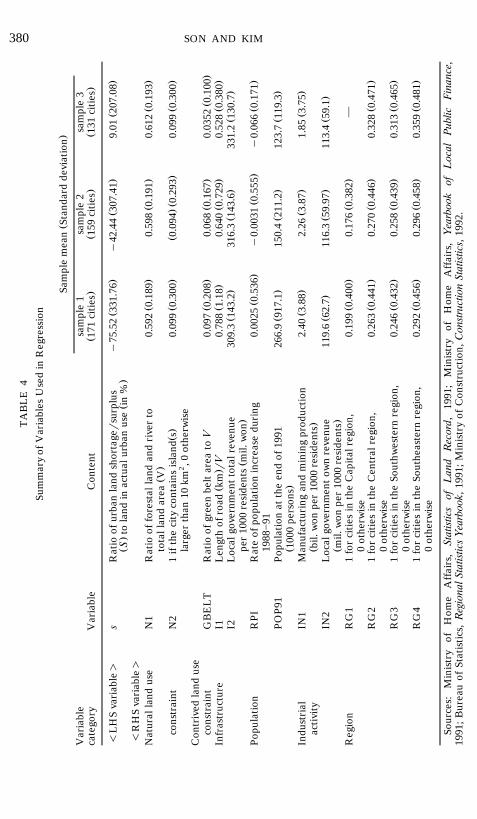
Definitions of all variables and their summary statistics are presented inTable 4.

3. Estimation Results

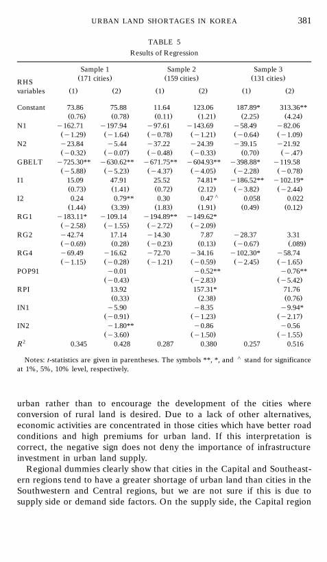
Estimated values of the coefficients of two sets of regression equationsare reported in Table 5 for each of the three samples described above.

Ž .Figures in column 1 are from the equation which has only supply sideŽ .factors as explanatory variables, and those in column 2 represent esti-

mates of regression equations which include demand side variables as well.The estimation results more or less support the hypothesis that only

government regulation can cause urban land shortages. Neither of twovariables for natural land use constraints proved significant at the 10%

Ž .level. Although N1 has fairly large t-values and expected y signs, naturalconstraints do not appear to be an important factor in explaining theurban land shortagersurplus in Korea. On the other hand, the regulatoryvariable GBELT exhibited a significant negative coefficient in five of sixcases. This appears to be a strong proof that regulations are at the root ofthe urban land shortage problem in Korean cities. It is also interesting tonote that the estimated coefficient of GBELT is much smaller in Sample 3than in the entire sample and Sample 2. It can be interpreted as implyingthat the greenbelt regulations have a binding impact mostly on the cities inthe Capital region and the six large cities.

There are a few cases where the sign of the coefficient differed from ourexpectation. Although infrastructure variable I2 had a positive sign in all

Ž .six cases only two being significant , the other infrastructure variable I1exhibited a significant negative coefficient in sub-sample 3 contrary to theexpectation that increased accessibility opens up prospects for develop-ment and decreases the shortage of urban land. This may be indicative ofthe infrastructure investment practice by which roads are built in order toalleviate congestion in cities where the land use is already predominantly

13 Ž .They are the Capital region Seoul, Inchon, and Kyunggi Province , the Central regionŽ .Taejeon, Kangwon Province, and North and South Choongchung provinces , the Southeast-

Ž .ern region Pusan, Taegu, and North and South Kyungsang provinces , and the SouthwesternŽ .region Kwangju, North and South Cholla provinces, and Cheju Province .

SON AND KIM380T

AB

LE

4Su

mm

ary

ofV

aria

bles

Use

din

Reg

ress

ion

Ž.

Sam

ple

mea

nSt

anda

rdde

viat

ion

Var

iabl

esa

mpl

e1

sam

ple

2sa

mpl

e3

Ž.

Ž.

Ž.

cate

gory

Var

iabl

eC

onte

nt17

1ci

ties

159

citie

s13

1ci

ties

Ž.

Ž.

Ž.

-L

HS

vari

able

)s

Rat

ioof

urba

nla

ndsh

orta

gers

urpl

usy

75.5

233

1.76

y42

.44

307.

419.

0120

7.08

Ž.

Ž.

Sto

land

inac

tual

urba

nus

ein

%-

RH

Sva

riab

le)

Ž.

Ž.

Ž.

Nat

ural

land

use

N1

Rat

ioof

fore

stal

land

and

rive

rto

0.59

20.

189

0.59

80.

191

0.61

20.

193

Ž.

tota

llan

dar

eaV

Ž.

Ž.

Ž.Ž

.Ž

.co

nstr

aint

N2

1if

the

city

cont

ains

isla

nds

0.09

90.

300

0.09

40.

293

0.09

90.

300

2la

rger

than

10km

,0ot

herw

ise

Con

triv

edla

ndus

eŽ

.Ž

.Ž

.co

nstr

aint

GB

EL

TR

atio

ofgr

een

belt

area

toV

0.09

70.

208

0.06

80.

167

0.03

520.

100

Ž.

Ž.

Ž.

Ž.

Infr

astr

uctu

reI1

Len

gth

ofro

adkm

rV0.

788

1.18

0.64

00.

729

0.52

80.

380

Ž.

Ž.

Ž.

I2L

ocal

gove

rnm

entt

otal

reve

nue

309.

314

3.2

316.

314

3.6

331.

213

0.7

Ž.

per

1000

resi

dent

sm

il.w

onŽ

.Ž

.Ž

.Po

pula

tion

RPI

Rat

eof

popu

latio

nin

crea

sedu

ring

0.00

250.

536

y0.

0031

0.55

5y

0.06

60.

171

1988

]91

Ž.

Ž.

Ž.

POP9

1Po

pula

tion

atth

een

dof

1991

266.

991

7.1

150.

421

1.2

123.

711

9.3

Ž.

1000

pers

ons

Ž.

Ž.

Ž.

Indu

stri

alIN

1M

anuf

actu

ring

and

min

ing

prod

uctio

n2.

403.

882.

263.

871.

853.

75Ž

.ac

tivity

bil.

won

per

1000

resi

dent

sŽ

.Ž

.Ž

.IN

2L

ocal

gove

rnm

ent

own

reve

nue

119.

662

.711

6.3

59.9

711

3.4

59.1

Ž.

mil.

won

per

1000

resi

dent

sŽ

.Ž

.R

egio

nR

G1

1fo

rci

ties

inth

eC

apita

lreg

ion,

0.19

90.

400

0.17

60.

382

}0

othe

rwis

eŽ

.Ž

.Ž

.R

G2

1fo

rci

ties

inth

eC

entr

alre

gion

,0.

263

0.44

10.

270

0.44

60.

328

0.47

10

othe

rwis

eŽ

.Ž

.Ž

.R

G3

1fo

rci

ties

inth

eSo

uthw

este

rnre

gion

,0.

246

0.43

20.

258

0.43

90.

313

0.46

50

othe

rwis

eŽ

.Ž

.Ž

.R

G4

1fo

rci

ties

inth

eSo

uthe

aste

rnre

gion

,0.

292

0.45

60.

296

0.45

80.

359

0.48

10

othe

rwis

e

Sour

ces:

Min

istr

yof

Hom

eA

ffai

rs,

Stat

istic

sof

Lan

dR

ecor

d,19

91;

Min

istr

yof

Hom

eA

ffai

rs,

Yea

rboo

kof

Loc

alP

ublic

Fin

ance

,19

91;B

urea

uof

Stat

istic

s,R

egio

nalS

tatis

tics

Yea

rboo

k,19

91;M

inis

try

ofC

onst

ruct

ion,

Con

stru

ctio

nSt

atis

tics,

1992

.


TABLE 5Results of Regression

Sample 1 Sample 2 Sample 3Ž . Ž . Ž .171 cities 159 cities 131 citiesRHS

Ž . Ž . Ž . Ž . Ž . Ž .variables 1 2 1 2 1 2

Constant 73.86 75.88 11.64 123.06 187.89* 313.36**Ž . Ž . Ž . Ž . Ž . Ž .0.76 0.78 0.11 1.21 2.25 4.24

N1 y162.71 y197.94 y97.61 y143.69 y58.49 y82.06Ž . Ž . Ž . Ž . Ž . Ž .y1.29 y1.64 y0.78 y1.21 y0.64 y1.09

N2 y23.84 y5.44 y37.22 y24.39 y39.15 y21.92Ž . Ž . Ž . Ž . Ž . Ž .y0.32 y0.07 y0.48 y0.33 0.70 y.47

GBELT y725.30** y630.62** y671.75** y604.93** y398.88* y119.58Ž . Ž . Ž . Ž . Ž . Ž .y5.88 y5.23 y4.37 y4.05 y2.28 y0.78

I1 15.09 47.91 25.52 74.81* y186.52** y102.19*Ž . Ž . Ž . Ž . Ž . Ž .0.73 1.41 0.72 2.12 y3.82 y2.44

nI2 0.24 0.79** 0.30 0.47 0.058 0.022Ž . Ž . Ž . Ž . Ž . Ž .1.44 3.39 1.83 1.91 0.49 0.12

RG1 y183.11* y109.14 y194.89** y149.62*Ž . Ž . Ž . Ž .y2.58 y1.55 y2.72 y2.09

RG2 y42.74 17.14 y14.30 7.87 y28.37 3.31Ž . Ž . Ž . Ž . Ž . Ž .y0.69 0.28 y0.23 0.13 y0.67 .089

RG4 y69.49 y16.62 y72.70 y34.16 y102.30* y58.74Ž . Ž . Ž . Ž . Ž . Ž .y1.15 y0.28 y1.21 y0.59 y2.45 y1.65

POP91 y0.01 y0.52** y0.76**Ž . Ž . Ž .y0.43 y2.83 y5.42

RPI 13.92 157.31* 71.76Ž . Ž . Ž .0.33 2.38 0.76

IN1 y5.90 y8.35 y9.94*Ž . Ž . Ž .y0.91 y1.23 y2.17

IN2 y1.80** y0.86 y0.56Ž . Ž . Ž .y3.60 y1.50 y1.55

2R 0.345 0.428 0.287 0.380 0.257 0.516

Notes: t-statistics are given in parentheses. The symbols **, *, and n stand for significanceat 1%, 5%, 10% level, respectively.

urban rather than to encourage the development of the cities whereconversion of rural land is desired. Due to a lack of other alternatives,economic activities are concentrated in those cities which have better roadconditions and high premiums for urban land. If this interpretation iscorrect, the negative sign does not deny the importance of infrastructureinvestment in urban land supply.

Regional dummies clearly show that cities in the Capital and Southeast-ern regions tend to have a greater shortage of urban land than cities in theSouthwestern and Central regions, but we are not sure if this is due tosupply side or demand side factors. On the supply side, the Capital region

SON AND KIM382

is subject to the Capital region growth control measures, in addition to thegreenbelt regulation and other nationwide land use regulations. Citiesaround Pusan and Taegu in the Southeastern region also have extensivegreenbelts. On the demand side, industrial, financial, administrative, andother urban activities are highly concentrated in the two regions.

The null hypothesis that all demand side variables jointly have no impacton the shortage of urban land was rejected by an F-test at 1% level ofsignificance in all three samples. Individually, the rate of populationincrease RPI has a positive coefficient, and population size POP91 has anegative coefficient. The former runs contrary to our expectation, but themagnitude is too small to be meaningful. While the latter is consistent withour expectation, the coefficient is not significant in one out of three cases.Industrial production IN1 in general shows negative signs with fairly larget-values. The coefficient is especially large and significant at the 1% levelfor Sample 3. It indicates that the urban land supply is not meeting thedemand for industrial development in small cities. Local government ownrevenue IN2 is negative and significant for Sample 1, but is not significantfor Sample 3.

These results have at least two policy implications. First, land useregulations rather than natural conditions are the main problem in urbanland supply. Removing the artificial constraint should be a preferredalternative in meeting the demand for urban land necessary to facilitateeconomic development and improve urban housing conditions. Second,infrastructure investment may be late and insufficient. Forward-lookingphysical planning will be necessary for forecasting the future and meetingthe demands before bottlenecks build up.

V. CONCLUDING REMARKS

The main objective of this study was to derive measures of shortage orsurplus of urban land from the standard urban model and to provideestimates of the measures for Korean cities. For each of 171 cities, weestimated urban and non-urban land price gradients and used the esti-mates to compute the equilibrium amount of urban land, paying dueattention to urban topography. We then calculated urban land shortagersurplus and found that 60 out of 171 cities have shortages whereas theremaining 111 cities have surpluses. The shortages appear to be mostserious for the six largest cities and cities in Kyunggi Province.

The model we used to estimate the shortage and surplus of urban landin Korean cities is based on a set of assumptions, some of which could bechallenged on conceptual and empirical grounds. Most importantly, severeland shortages found in large cities may be interpreted as rejecting themonocentric model and having nothing to say about land shortagersurplus


situations.14 Although we have tried to rectify some of the potentialproblems, it is difficult to tell to what extent they have affected theaccuracy of our estimation. On the other hand, we believe that our studyperhaps represents the first serious attempt to apply the land price data tomeasure the size of discrepancy between optimum and actual amount ofurban land.

We also investigated the determinants of shortagersurplus of urbanland. Our results suggest that land use regulations such as greenbelt arethe dominant cause of urban land shortages. This has an obvious policyimplication that land use regulations should be relaxed in order to satisfythe increasing demand for urban land and stabilize land prices in Koreancities.

Some variables turned out to affect the magnitude of urban landshortagersurplus in ways which are different from our expectations. Wealso found that the some demand side variables have a significant effect onthe urban land shortagersurplus, contrary to the implication of the small-and-open city assumption. An analysis of the mechanisms for such interac-tion would be a topic for further research.

14 A different model of multiple centers would be more appropriate for Seoul and satellitecities as was pointed out by a referee. Unfortunately, however, our data set did not containdistance to downtown Seoul from plots located in satellite cities.

REFERENCES

1. J. K. Brueckner, The structure of urban equilibria: A unified treatment of Muth]MillsŽ .model, in ‘‘Handbook of Regional and Urban Economics,’’ Vol. II E. S. Mills, Ed. ,

Ž .North Holland, New York 1987 .2. L. M. Hannah, K.-H. Kim, and E. S. Mills, Land use controls and housing prices in

Ž .Korea, Urban Studies, 30, 147]156 1993 .3. C.-H. Kim, Land Use Regulations in Korea, Korea Economic Research Institute, Seoul

Ž . Ž .1994 . In Korean.4. K.-H. Kim, Housing prices, affordability, and government policy in Korea, Journal of Real

Ž .Estate Economics and Finance, 6, 55]71 1993 .5. C.-M. Lee, ‘‘Greenbelt Impacts on Dynamics of a Physical Urban Development and Land

Market: A Welfare Analysis}The Case of Seoul’s Greenbelt,’’ unpublished doctoralŽ .dissertation, University of Pennsylvania, Philadelphia 1994 .

6. J. F. McDonald, Econometric studies of urban population density: A survey, Journal ofŽ .Urban Economics, 26, 361]385 1989 .

SON AND KIM384

7. D. P. McMillen and J. F. McDonald, Urban land value functions with endogenous zoning,Ž .Journal of Urban Economics, 29, 14]27 1991 .

8. H. O. Pollakowski and S. M. Wachter, The effects of land-use constraints on housingŽ .prices, Land Economics, 66, 315]324 1990 .

9. H. W. Richardson, Monocentric vs. policentric models: The future of urban economics inŽ .regional science, Annals of Regional Science, 22, 1]12 1989 .

10. L. A. Rose, Topographical constraints and urban land supply indexes, Journal of UrbanŽ .Economics, 26, 325]345 1989 .

11. J. Yinger, Urban models with more than one employment center, Journal of UrbanŽ .Economics, 31, 181]205 1992 .

Documents

Analysis of Urban Land Shortages: The Case of Korean Citieshompi.sogang.ac.kr/kyungkim/freeboard/papers/An... · Analysis of Urban Land Shortages: The Case of Korean Cities* Jae-Young