Analysis of Two Phase Flow Pattern maps - Energetické · PDF fileDigitized Shell’s DEP 31.22.05.11 map 4.1 Description of the map This map was created by the company Shell ... Analysis

Brno University of Technology

Faculty of Mechanical Engineering

Energy Institute

Analysis of Two-Phase Flow Pattern Maps

Report: 16-09 / 14

Elaborated by: Noé Pinto del Corral

Revised:

Brno, September 2014

INDEX

1. Oshinowo–Charles’s maps ................................................................................................................ 3

1.1 Description of the map ................................................................................................................ 3

1.2. Properties of the experiment. Limitations of the map ............................................................. 4

2. Hewitt and Roberts’s map ................................................................................................................. 6


2.2. Properties of the experiment. Limitations of the map ............................................................. 6

3. Taitel and Dukler’s map .................................................................................................................... 8


3.2 Properties of the experiment. Limitations of the map .............................................................. 9

4. Digitized Shell’s DEP 31.22.05.11 map ........................................................................................... 11

4.1 Description of the map .............................................................................................................. 11

4.2 Properties of the experiment. Limitations of the map ............................................................ 12

5. Griffith and Wallis’s map ................................................................................................................. 14


5.2 Properties of the experiment. Limitations of the map. ........................................................... 14

6. Golan and Stenning’s map ............................................................................................................... 16



7. Mandhane-Gregory-Aziz’s map ...................................................................................................... 18



8. Baker’s map ...................................................................................................................................... 20



9. Conclusions and recommendations ............................................................................................... 24

10. References ...................................................................................................................................... 25

Noé Pinto del Corral Analysis of Two-Phase Flow Pattern Maps

3

1. Oshinowo–Charles’s maps

1.1 Description of the map

Oshinowo-Charles (Oshinowo and Charles, 1974) suggested by experiment that the flow patterns

depend on the volumetric flow rate of the gas flow and other fluid dynamic properties similar to

the other maps. Therefore, the flow pattern can be estimated through Eqs. 1–3.

Figure 1.Oshinowo-Charles’s map for up-flow vertical flux (Oshinowo and Charles, 1974).

Figure 2.Oshinowo-Charles’s map for down-flow vertical flux (Oshinowo and Charles, 1974).


4

𝑅𝑣 =𝑄𝐺

𝑄𝐿=

𝑢𝐺

𝑢𝐿 [–] (1)

𝐹𝑟𝑇𝑃 =(𝑢𝐺+𝑢𝐿)2

𝑔∙𝐷 [–] (2)

𝛬 =𝜇𝐿

𝜇𝑤[

𝜌𝐿

𝜌𝑤(

𝜎𝐿

𝜎𝑤)

3]

−1/4

[–] (3)

𝑄𝐺 is the volumetric flow rate of the gas, 𝑄𝐿 is the volumetric flow rate of the liquid, 𝐹𝑟𝑇𝑃 is the

Froude number of the two phases, ug and ul are the gas and liquid superficial velocities

respectively.

1.2. Properties of the experiment. Limitations of the map

*Properties of the pipe:

-Length: 5.273 m

-Diameter: 2.54 cm

*Pressure: 0.71 barg

*Volumetric flux range for gas: 0 – 6.7 ∙ 105 kg/m3h

*Volumetric flux range for liquid: 1.35 ∙ 105 – 2.4 ∙ 107 kg/m3h

*Gas flow rate range: 1 – 104 kg/h

*Liquid flow rate range: 19 – 3540 kg/h

*Liquid density range: 1000 – 1250 kg/m3

*Liquid viscosity range (water–glycerin solutions): 1 ∙ 10−3 – 12 ∙ 10−3 kg/m s

*Surface tension: 68 ∙ 10−3 – 73 ∙ 10−3 kg/s2

*Temperature range: 10 – 27 °C

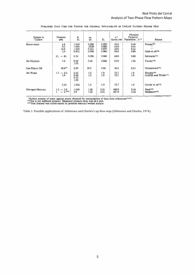
These were the conditions on which the experiment was done, but the authors have tested the up-

flow map also with other data (from other authors), so maybe we could assume that the map is

also valid for the following conditions (Oshinowo and Charles, 1974):


5

Table 1. Possible applications of Oshinowo and Charles’s up-flow map (Oshinowo and Charles, 1974).


6

2. Hewitt and Roberts’s map


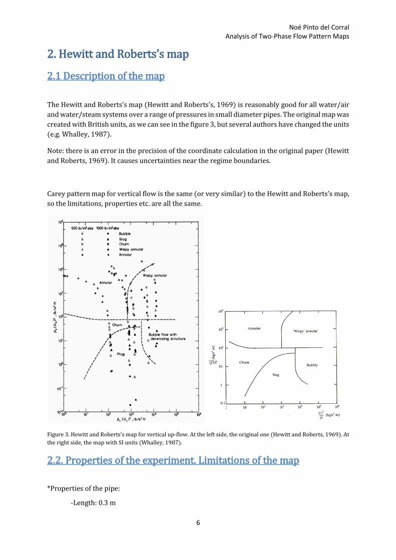
The Hewitt and Roberts’s map (Hewitt and Roberts’s, 1969) is reasonably good for all water/air

and water/steam systems over a range of pressures in small diameter pipes. The original map was

created with British units, as we can see in the figure 3, but several authors have changed the units

(e.g. Whalley, 1987).

Note: there is an error in the precision of the coordinate calculation in the original paper (Hewitt

and Roberts, 1969). It causes uncertainties near the regime boundaries.

Carey pattern map for vertical flow is the same (or very similar) to the Hewitt and Roberts’s map,

so the limitations, properties etc. are all the same.

Figure 3. Hewitt and Roberts’s map for vertical up-flow. At the left side, the original one (Hewitt and Roberts, 1969). At

the right side, the map with SI units (Whalley, 1987).

2.2. Properties of the experiment. Limitations of the map


-Length: 0.3 m


7

-Diameter: 31.75 mm

*Range of pressures at the mixing zone:

- Absolute pressure: 14.27 ∙ 104 Pa – 54.26 ∙ 104 Pa

- Relative pressure (P0 – Patm): 4.14 ∙ 104 Pa – 44.13 ∙ 104 Pa

There also some experiments at higher pressures (500 and 1000 psig), showed in figure 3.

*Range of temperatures:

- Temperature of the gas: 18.9°C – 25.3°C

- Temperature of the liquid: 20.8°C – 32.5°C

*Flow rates range:

- Gas: 1.36 kg/h – 544.3 kg/h

- Liquid: 226.8 kg/h – 8164.7 kg/h

*Properties of the substances (Basically they consist in water/air or water/steam systems):

-Gas density range: 1.68 kg/m3 – 6.4 kg/m3

-Liquid density range: 992.2 kg/m3 – 997.8 kg/m3


8

3. Taitel and Dukler’s map


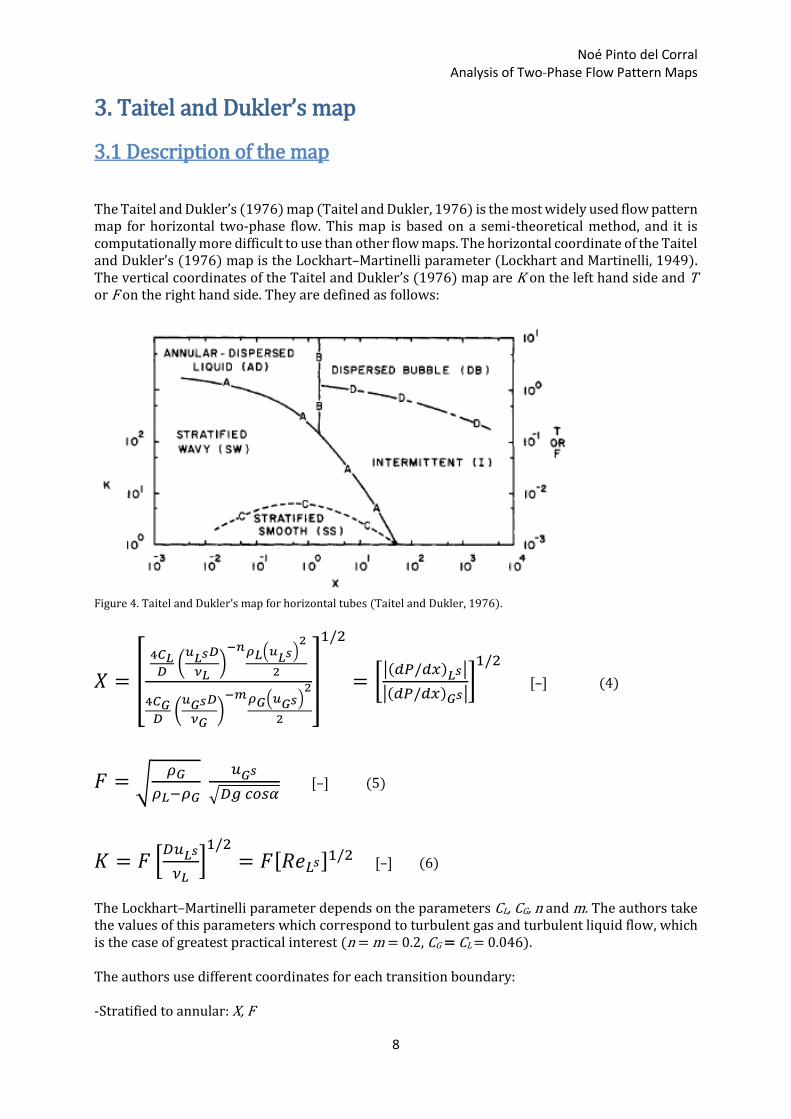
The Taitel and Dukler’s (1976) map (Taitel and Dukler, 1976) is the most widely used flow pattern map for horizontal two-phase flow. This map is based on a semi-theoretical method, and it is computationally more difficult to use than other flow maps. The horizontal coordinate of the Taitel and Dukler’s (1976) map is the Lockhart–Martinelli parameter (Lockhart and Martinelli, 1949). The vertical coordinates of the Taitel and Dukler’s (1976) map are K on the left hand side and T or F on the right hand side. They are defined as follows:

Figure 4. Taitel and Dukler’s map for horizontal tubes (Taitel and Dukler, 1976).

𝑋 = [

4𝐶𝐿𝐷

(𝑢

𝐿𝑠𝐷

𝜈𝐿)

−𝑛𝜌𝐿(𝑢𝐿𝑠)

2

2

4𝐶𝐺𝐷

(𝑢𝐺𝑠𝐷

𝜈𝐺)

−𝑚𝜌𝐺(𝑢𝐺𝑠)2

2

]

1/2

= [|(𝑑𝑃/𝑑𝑥)𝐿𝑠|

|(𝑑𝑃/𝑑𝑥)𝐺𝑠|]

1/2

[–] (4)

𝐹 = √𝜌𝐺

𝜌𝐿−𝜌𝐺

𝑢𝐺𝑠

√𝐷𝑔 𝑐𝑜𝑠𝛼 [–] (5)

𝐾 = 𝐹 [𝐷𝑢𝐿𝑠

𝜈𝐿]

1/2= 𝐹[𝑅𝑒𝐿𝑠]1/2 [–] (6)

The Lockhart–Martinelli parameter depends on the parameters CL, CG, n and m. The authors take the values of this parameters which correspond to turbulent gas and turbulent liquid flow, which is the case of greatest practical interest (n = m = 0.2, CG = CL = 0.046). The authors use different coordinates for each transition boundary: -Stratified to annular: X, F


9

-Stratified to intermittent: X, F -Intermittent to dispersed bubble: X, T -Stratified smooth to stratified wavy: X, K

3.2 Properties of the experiment. Limitations of the map

In principle, the map was developed using theoretical methods, so it should not have the restrictions of the experimental ones. Nevertheless, there have been taken some theoretical assumptions that could affect the accordance between some experiments and the Taitel and Dukler’s map. Here we have some of these assumptions:

(a) The map was developed for Newtonian liquid–gas mixtures

(b) They assume that hydraulic gradient in the liquid is negligible at transition conditions.

(c) They use the Gazley criteria (Gazley, 1949) for smooth stratified flow (see Taitel and Dukler, 1976 for details)

(d) They use n =m=0.2 and CG =CL=0.046 which corresponds to turbulent gas and turbulent liquid.

(e) They use the following criteria for Stratified to Intermittent transition (see Taitel and Dukler, 1976, for details):

𝐹2 [1

𝐶22

𝑢𝐺 𝑑�̃�𝐿/𝑑ℎ̃𝐿

�̃�𝐺] ≥ 1 (7)

where F is a Froude number modified by the density ratio:

𝐹 = √𝜌𝐺

𝜌𝐿−𝜌𝐺

𝑢𝐺𝑠

√𝐷𝑔 𝑐𝑜𝑠𝛼 [–] (8)

(f) They fix the transition between intermittent and Annular Dispersed in the following way: ℎ𝐿

𝐷= 0.5 → 𝑋 = 1.6 [–] (9)

(g) Transition between stratified smooth and stratified wavy is given by:

𝐾 ≥2

√𝑢𝐿 𝑢𝐺√𝑠 (10)

(h) Transition between intermittent and dispersed bubble is:


10

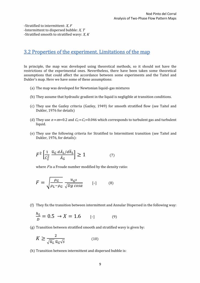
𝑇2 ≥ [8�̃�𝐺

�̃�𝑖𝑢𝐿2(𝑢𝐿�̃�𝐿)−𝑛

] (11)

This map has been tested by the authors with the Mandhane et al. experimental data, showing a

great accordance.


11

4. Digitized Shell’s DEP 31.22.05.11 map


This map was created by the company Shell (Shell company, 2007), for transport (charge and

discharge) of combustibles. The flow maps are generalized by using as parameters the gas and

liquid Froude number respectively, based on the feed pipe velocity and diameter.

The gas and liquid Froude numbers are defined as follows:

-Gas Froude number

𝐹𝑟𝐺 = 𝑢𝐺√𝜌𝐺

(𝜌𝐿−𝜌𝐺)𝑔𝑑𝑓𝑝 [–] (12)

-Liquid Froude number

𝐹𝑟𝐿 = 𝑢𝐿√𝜌𝐿

(𝜌𝐿−𝜌𝐺)𝑔𝑑𝑓𝑝 [–] (13)

In the above formulae, ug and ul are the superficial gas and liquid velocity respectively in the feed

pipe, and dfp is the inner diameter of the feed pipe.

𝑢𝐺 =𝑄𝐺

(𝜋𝑑𝑓𝑝2 /4)

[m/s] (14)

𝑢𝐿 =𝑄𝐿

(𝜋𝑑𝑓𝑝2 /4)

[m/s] (15)

and the averaged liquid density ρL is defined as:

𝜌𝐿 =𝑀𝐿

𝑄𝐿 [kg/m3 ] (16)


12

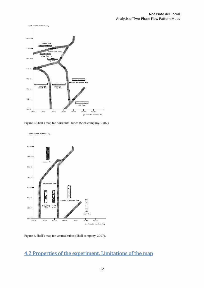
Figure 5. Shell’s map for horizontal tubes (Shell company, 2007).

Figure 6. Shell’s map for vertical tubes (Shell company, 2007).



13

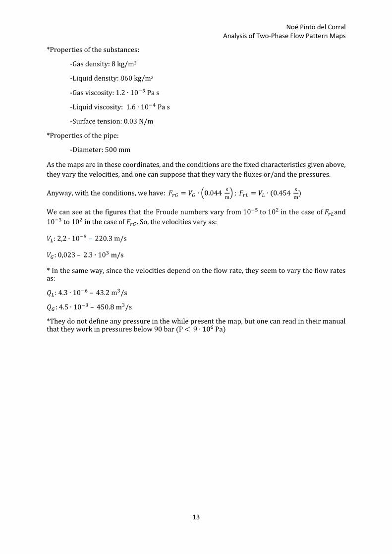
*Properties of the substances:

-Gas density: 8 kg/m3

-Liquid density: 860 kg/m3

-Gas viscosity: 1.2 ∙ 10−5 Pa s

-Liquid viscosity: 1.6 ∙ 10−4 Pa s

-Surface tension: 0.03 N/m


-Diameter: 500 mm

As the maps are in these coordinates, and the conditions are the fixed characteristics given above,

they vary the velocities, and one can suppose that they vary the fluxes or/and the pressures.

Anyway, with the conditions, we have: 𝐹𝑟𝐺 = 𝑉𝐺 ∙ (0.044 s

m) ; 𝐹𝑟𝐿 = 𝑉𝐿 ∙ (0.454

s

m)

We can see at the figures that the Froude numbers vary from 10−5 to 102 in the case of 𝐹𝑟𝐿and

10−3 to 102 in the case of 𝐹𝑟𝐺 . So, the velocities vary as:

𝑉𝐿: 2,2 ∙ 10−5 – 220.3 m/s

𝑉𝐺: 0,023 – 2.3 ∙ 103 m/s

* In the same way, since the velocities depend on the flow rate, they seem to vary the flow rates as:

𝑄𝐿: 4.3 ∙ 10−6 – 43.2 m3/s

𝑄𝐺: 4.5 ∙ 10−3 – 450.8 m3/s

*They do not define any pressure in the while present the map, but one can read in their manual that they work in pressures below 90 bar (P < 9 ∙ 106 Pa)


14

5. Griffith and Wallis’s map


Griffith and Wallis’s map (Griffith et al., 1959) was originally created for the study of slug flow in

vertical direction. Therefore, the map shows the region in which the slug flow appears, but one

cannot really trust in which the map says about the other patterns, since they do not have any

experimental points in these areas (see Golan and Stenning, 1969).

The axes of this map were defined as follows:

Y axis: 𝑄𝑔

𝑄𝑙+𝑄𝑔 [–]

X axis: (𝑄𝑙+𝑄𝑔

𝐴𝑝)

2

/𝑔𝐷𝑝 [–]

Where, Qg and Ql are the gas and liquid volumetric flow rate respectively, Ap is the cross-section

area of the pipe, Dp is the diameter of the pipe and g is the acceleration of gravity

Figure 7: Griffith and Wallis’s map (Griffith et al., 1959).

5.2 Properties of the experiment. Limitations of the map.

*Liquid used: water

*Gas used: air


-Length: 5.48 m


15

-Diameter: 1.27 – 2.54 cm


*Liquid density: 1000 kg/m3

*Liquid viscosity: 1 ∙ 10−3 kg/m s

*Surface tension: 73 ∙ 10−3 kg/s2


16

6. Golan and Stenning’s map


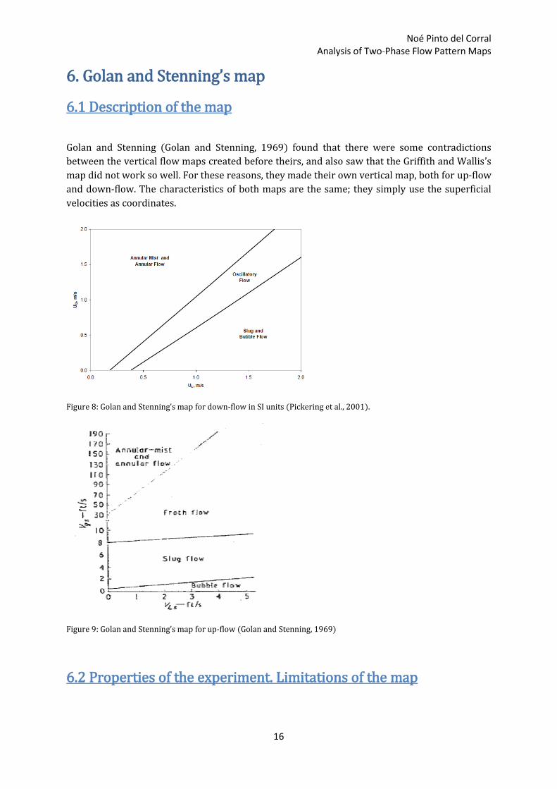
Golan and Stenning (Golan and Stenning, 1969) found that there were some contradictions

between the vertical flow maps created before theirs, and also saw that the Griffith and Wallis’s

map did not work so well. For these reasons, they made their own vertical map, both for up-flow

and down-flow. The characteristics of both maps are the same; they simply use the superficial

velocities as coordinates.

Figure 8: Golan and Stenning’s map for down-flow in SI units (Pickering et al., 2001).

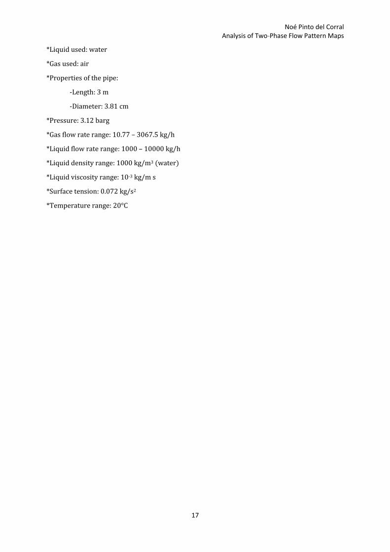
Figure 9: Golan and Stenning’s map for up-flow (Golan and Stenning, 1969)



17

*Liquid used: water

*Gas used: air


-Length: 3 m

-Diameter: 3.81 cm


*Gas flow rate range: 10.77 – 3067.5 kg/h

*Liquid flow rate range: 1000 – 10000 kg/h

*Liquid density range: 1000 kg/m3 (water)

*Liquid viscosity range: 10-3 kg/m s

*Surface tension: 0.072 kg/s2

*Temperature range: 20°C


18

7. Mandhane-Gregory-Aziz’s map


Mandhane et al. (Mandhane et al., 1974) realized that there were a lot of contradictions between

the proposed maps until that moment, so they try to re-evaluate them with a very big amount of

data. The used a data bank which has near 14000 experimental data from research results since

1962 until 1973 (AGA-API Two-Phase Flow Data Bank). They took all the results of horizontal

flow and defined their own map.

Following their research, it seems that Baker’s map (Baker, 1954) is not good enough, even if it is

quite used in some industries.

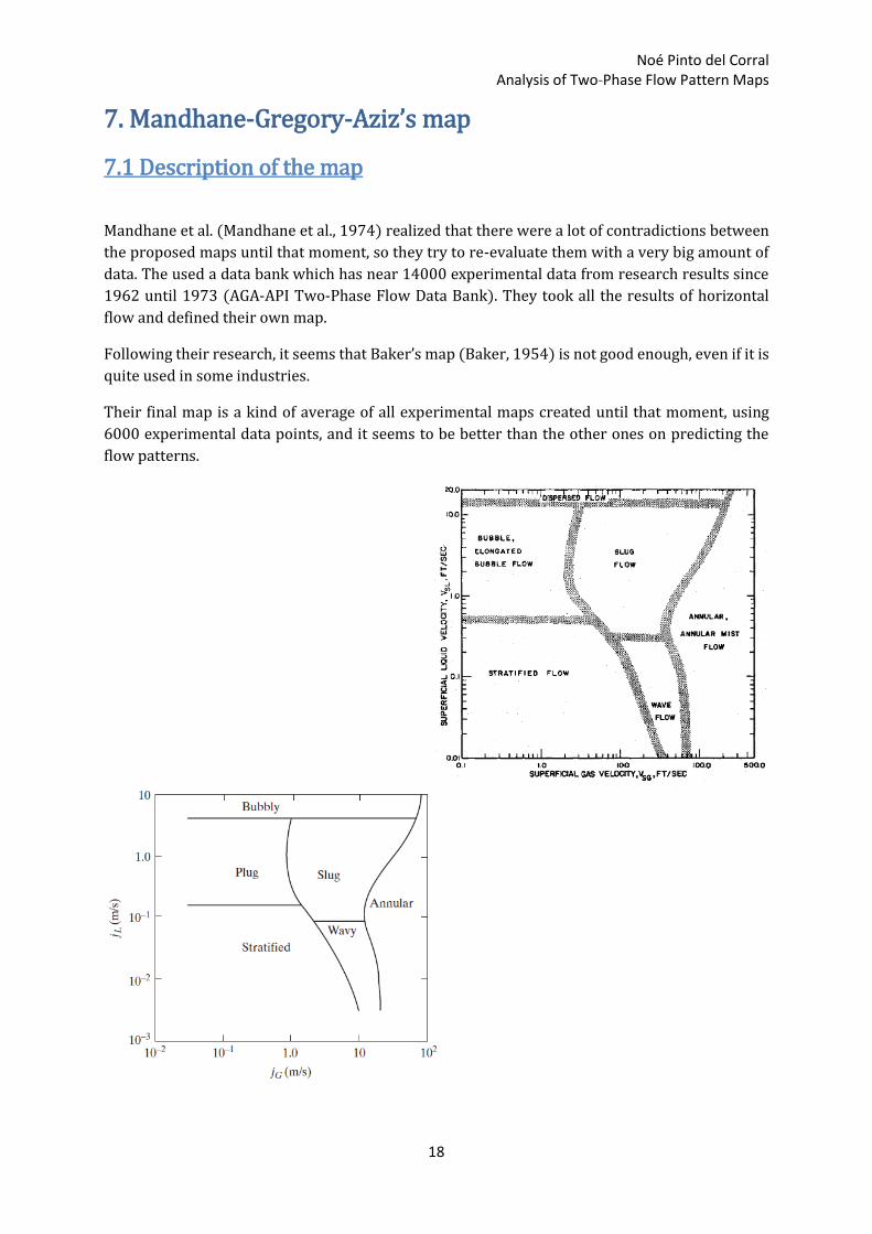
Their final map is a kind of average of all experimental maps created until that moment, using

6000 experimental data points, and it seems to be better than the other ones on predicting the

flow patterns.


19

Figure 10: Mandhane-Gregory-Aziz’s map for horizontal flow the upper one is the original (Mandhane et al., 1974), the

second one is the same with SI units (Ghiaasiaan, 2008).


In this case, there is not only one experiment, but one can read, in the Mandhane et al. paper, the

ranges of some of the parameters that we need. The map works better for water-air systems and

pipe diameters less than 5 cm. This is because most of the data that they took had these properties.

Instead of that, the map works also well in the whole range defined below:

*Pipe diameter: 1.27 – 16.51 cm

*Gas flow rate range: 1.82 ∙ 10−5 – 730 kg/h estimated

*Liquid flow rate range: 0.054 – 632.5 kg/h estimated

*Liquid density range: 704.8 – 1009.2 kg/m3

*Gas density range: 0.8 – 50.5 kg/m3

*Liquid viscosity range: 3 ∙ 10−4 – 0.09 kg/m s

*Gas viscosity range: 10−5 – 2.2 ∙ 10−5 kg/m s

*Surface tension range: 24 ∙ 10−3 – 0.1 kg/s2

*Superficial liquid velocity: 9 ∙ 10−4 – 7.32 m/s

*Superficial gas velocity: 0.043 – 170.7 m/s


20

8. Baker’s map


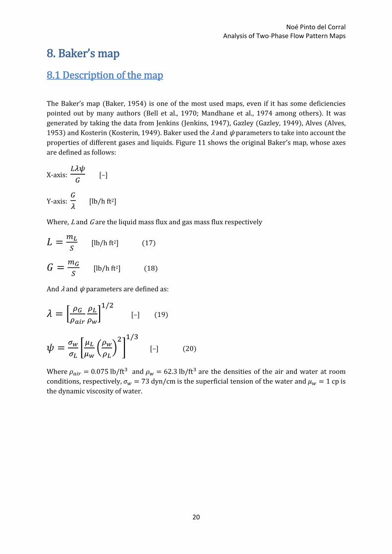
The Baker’s map (Baker, 1954) is one of the most used maps, even if it has some deficiencies

pointed out by many authors (Bell et al., 1970; Mandhane et al., 1974 among others). It was

generated by taking the data from Jenkins (Jenkins, 1947), Gazley (Gazley, 1949), Alves (Alves,

1953) and Kosterin (Kosterin, 1949). Baker used the λ and ψ parameters to take into account the

properties of different gases and liquids. Figure 11 shows the original Baker’s map, whose axes

are defined as follows:

X-axis: 𝐿𝜆𝜓

𝐺 [–]

Y-axis: 𝐺

𝜆 [lb/h ft2]

Where, L and G are the liquid mass flux and gas mass flux respectively

𝐿 =𝑚𝐿

𝑆 [lb/h ft2] (17)

𝐺 =𝑚𝐺

𝑆 [lb/h ft2] (18)

And λ and ψ parameters are defined as:

𝜆 = [𝜌𝐺

𝜌𝑎𝑖𝑟

𝜌𝐿

𝜌𝑤]

1/2 [–] (19)

𝜓 =𝜎𝑤

𝜎𝐿[

𝜇𝐿

𝜇𝑤(

𝜌𝑤

𝜌𝐿)

2]

1/3

[–] (20)

Where 𝜌𝑎𝑖𝑟 = 0.075 lb/ft3 and 𝜌𝑤 = 62.3 lb/ft3 are the densities of the air and water at room

conditions, respectively, 𝜎𝑤 = 73 dyn/cm is the superficial tension of the water and 𝜇𝑤 = 1 cp is

the dynamic viscosity of water.


21

Figure 11: Original Baker’s map for horizontal flow (Baker, 1954).

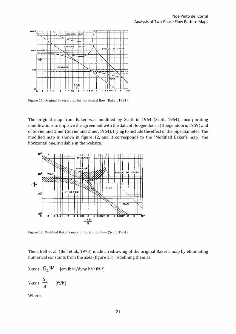
The original map from Baker was modified by Scott in 1964 (Scott, 1964), incorporating

modifications to improve the agreement with the data of Hoogendoorn (Hoogendoorn, 1959) and

of Govier and Omer (Govier and Omer, 1964), trying to include the effect of the pipe diameter. The

modified map is shown in figure 12, and it corresponds to the “Modified Baker’s map”, the

horizontal one, available in the website.

Figure 12: Modified Baker’s map for horizontal flow (Scott, 1964).

Then, Bell et al. (Bell et al., 1970) made a redrawing of the original Baker’s map by eliminating

numerical constants from the axes (figure 13), redefining them as:

X-axis: 𝐺𝐿𝛹 [cm lb2/3/dyne h4/3 ft1/3]

Y-axis: 𝐺𝑣

𝛬 [ft/h]

Where,


22

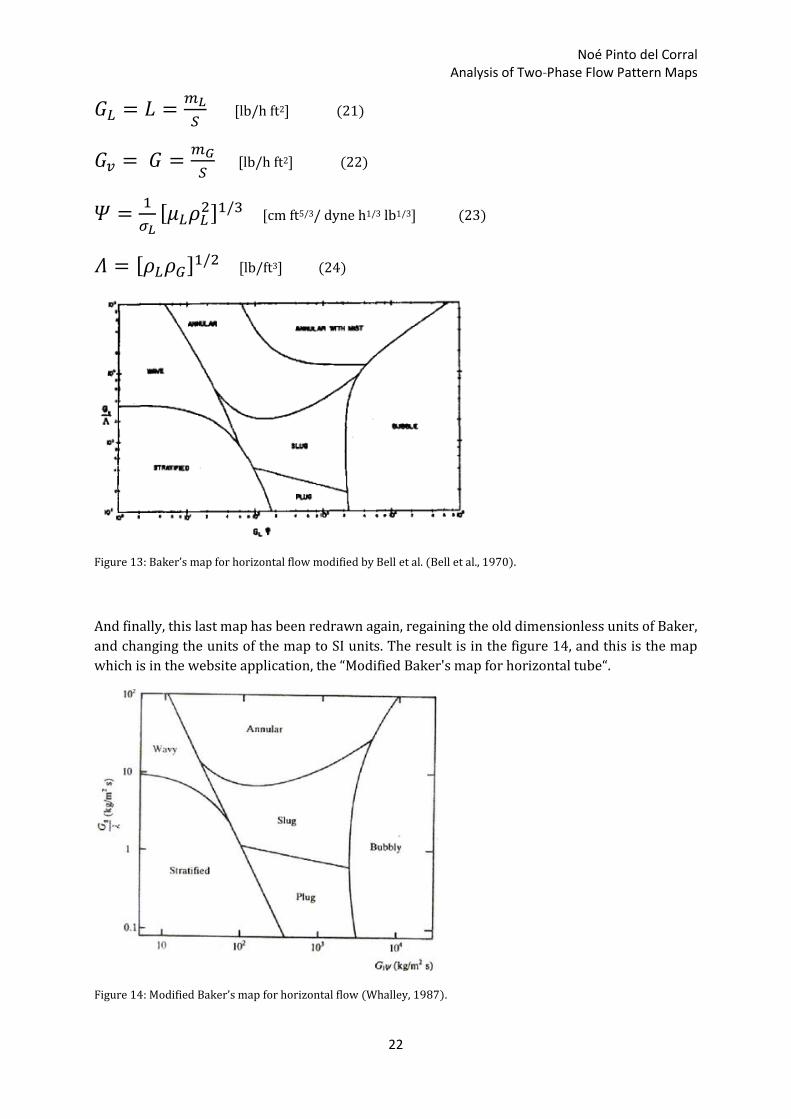
𝐺𝐿 = 𝐿 =𝑚𝐿

𝑆 [lb/h ft2] (21)

𝐺𝑣 = 𝐺 =𝑚𝐺

𝑆 [lb/h ft2] (22)

𝛹 =1

𝜎𝐿[𝜇𝐿𝜌𝐿

2]1/3 [cm ft5/3/ dyne h1/3 lb1/3] (23)

𝛬 = [𝜌𝐿𝜌𝐺]1/2 [lb/ft3] (24)

Figure 13: Baker’s map for horizontal flow modified by Bell et al. (Bell et al., 1970).

And finally, this last map has been redrawn again, regaining the old dimensionless units of Baker,

and changing the units of the map to SI units. The result is in the figure 14, and this is the map

which is in the website application, the “Modified Baker's map for horizontal tube“.

Figure 14: Modified Baker’s map for horizontal flow (Whalley, 1987).


23

The axes are given by a kind of combination of Bell’s and Baker’s coordinates:

X-axis: 𝐺𝐿𝜓 [kg/m2 s]

Y-axis: 𝐺𝑣

𝜆 [kg/m2 s]

Where 𝜆 and 𝜓 are the dimensionless Baker’s parameters defined in equations 19 and 20.


Baker’s map was made with the data of Jenkins (Jenkins, 1947), Gazley (Gazley, 1949), Alves

(Alves, 1953) and Kosterin (Kosterin, 1949), so he does not specify any experimental conditions

on his paper. Furthermore, the map has two different versions, one including the data from

Hoogendoorn (Hoogendoorn, 1959) and Govier and Omer (Govier and Omer, 1964), so we should

take this data into account as well. However, we can say, generally, that the map is reasonably

good for water/air and oil/gas mixtures in small diameter (< 0.05 m) pipes.

The map was developed using 1, 2 and 4-inch diameter pipe and air/water mixtures near

atmospheric pressures at a temperature of 68 degrees F:


-Diameter: 2.54 – 10.160 cm

*Pressure: 0 – 1 barg

*Liquid density: 1000 kg/m3

*Liquid viscosity: 1 ∙ 10−3 kg/m s

*Surface tension: 73 ∙ 10−3 kg/s2

*Temperature: 20 °C


24

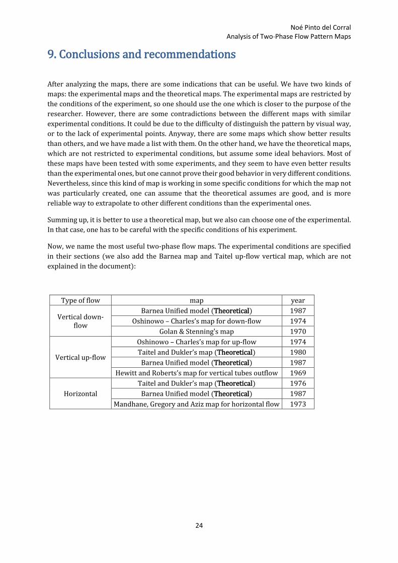
9. Conclusions and recommendations

After analyzing the maps, there are some indications that can be useful. We have two kinds of

maps: the experimental maps and the theoretical maps. The experimental maps are restricted by

the conditions of the experiment, so one should use the one which is closer to the purpose of the

researcher. However, there are some contradictions between the different maps with similar

experimental conditions. It could be due to the difficulty of distinguish the pattern by visual way,

or to the lack of experimental points. Anyway, there are some maps which show better results

than others, and we have made a list with them. On the other hand, we have the theoretical maps,

which are not restricted to experimental conditions, but assume some ideal behaviors. Most of

these maps have been tested with some experiments, and they seem to have even better results

than the experimental ones, but one cannot prove their good behavior in very different conditions.

Nevertheless, since this kind of map is working in some specific conditions for which the map not

was particularly created, one can assume that the theoretical assumes are good, and is more

reliable way to extrapolate to other different conditions than the experimental ones.

Summing up, it is better to use a theoretical map, but we also can choose one of the experimental.

In that case, one has to be careful with the specific conditions of his experiment.

Now, we name the most useful two-phase flow maps. The experimental conditions are specified

in their sections (we also add the Barnea map and Taitel up-flow vertical map, which are not

explained in the document):

Type of flow map year

Vertical down-flow

Barnea Unified model (Theoretical) 1987

Oshinowo – Charles’s map for down-flow 1974

Golan & Stenning's map 1970

Vertical up-flow

Oshinowo – Charles’s map for up-flow 1974

Taitel and Dukler’s map (Theoretical) 1980


Hewitt and Roberts’s map for vertical tubes outflow 1969

Horizontal

Taitel and Dukler’s map (Theoretical) 1976


Mandhane, Gregory and Aziz map for horizontal flow 1973


25

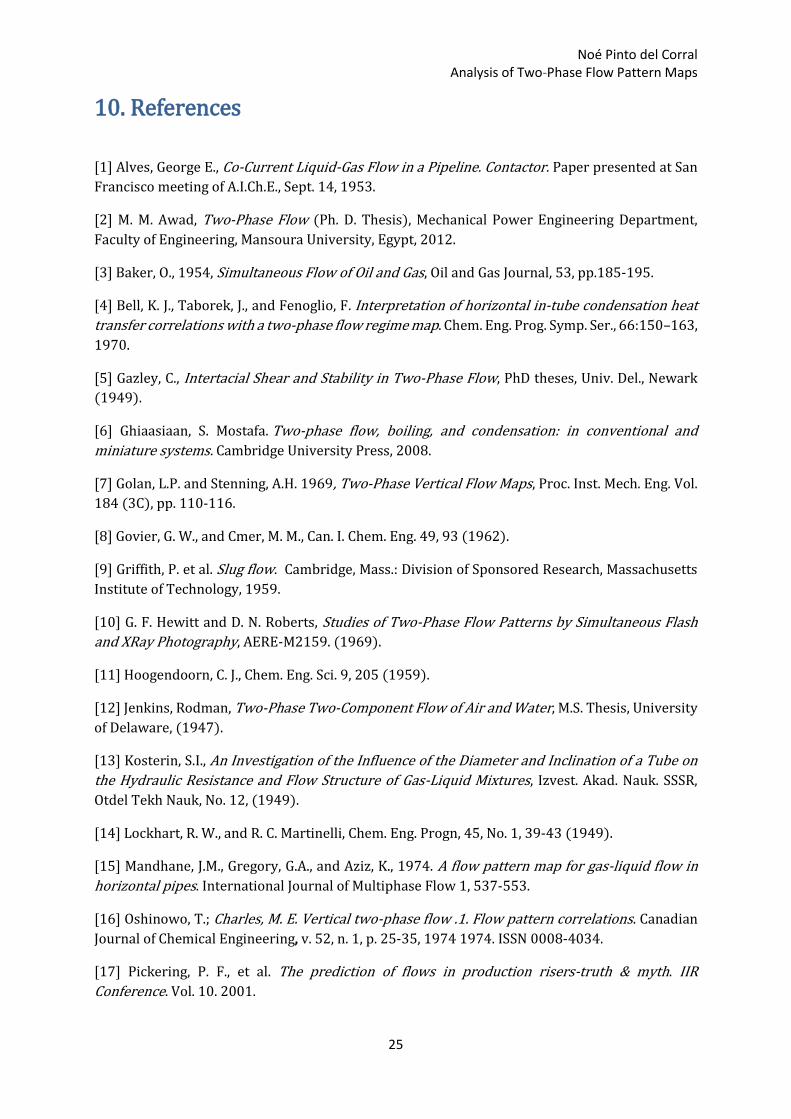
10. References

[1] Alves, George E., Co-Current Liquid-Gas Flow in a Pipeline. Contactor. Paper presented at San

Francisco meeting of A.I.Ch.E., Sept. 14, 1953.

[2] M. M. Awad, Two-Phase Flow (Ph. D. Thesis), Mechanical Power Engineering Department,

Faculty of Engineering, Mansoura University, Egypt, 2012.

[3] Baker, O., 1954, Simultaneous Flow of Oil and Gas, Oil and Gas Journal, 53, pp.185-195.

[4] Bell, K. J., Taborek, J., and Fenoglio, F. Interpretation of horizontal in-tube condensation heat

transfer correlations with a two-phase flow regime map. Chem. Eng. Prog. Symp. Ser., 66:150–163,

1970.

[5] Gazley, C., Intertacial Shear and Stability in Two-Phase Flow, PhD theses, Univ. Del., Newark

(1949).

[6] Ghiaasiaan, S. Mostafa. Two-phase flow, boiling, and condensation: in conventional and

miniature systems. Cambridge University Press, 2008.

[7] Golan, L.P. and Stenning, A.H. 1969, Two-Phase Vertical Flow Maps, Proc. Inst. Mech. Eng. Vol.

184 (3C), pp. 110-116.

[8] Govier, G. W., and Cmer, M. M., Can. I. Chem. Eng. 49, 93 (1962).

[9] Griffith, P. et al. Slug flow. Cambridge, Mass.: Division of Sponsored Research, Massachusetts

Institute of Technology, 1959.

[10] G. F. Hewitt and D. N. Roberts, Studies of Two-Phase Flow Patterns by Simultaneous Flash

and XRay Photography, AERE-M2159. (1969).

[11] Hoogendoorn, C. J., Chem. Eng. Sci. 9, 205 (1959).

[12] Jenkins, Rodman, Two-Phase Two-Component Flow of Air and Water, M.S. Thesis, University

of Delaware, (1947).

[13] Kosterin, S.I., An Investigation of the Influence of the Diameter and Inclination of a Tube on

the Hydraulic Resistance and Flow Structure of Gas-Liquid Mixtures, Izvest. Akad. Nauk. SSSR,

Otdel Tekh Nauk, No. 12, (1949).

[14] Lockhart, R. W., and R. C. Martinelli, Chem. Eng. Progn, 45, No. 1, 39-43 (1949).

[15] Mandhane, J.M., Gregory, G.A., and Aziz, K., 1974. A flow pattern map for gas-liquid flow in

horizontal pipes. International Journal of Multiphase Flow 1, 537-553.

[16] Oshinowo, T.; Charles, M. E. Vertical two-phase flow .1. Flow pattern correlations. Canadian

Journal of Chemical Engineering, v. 52, n. 1, p. 25-35, 1974 1974. ISSN 0008-4034.

[17] Pickering, P. F., et al. The prediction of flows in production risers-truth & myth. IIR

Conference. Vol. 10. 2001.


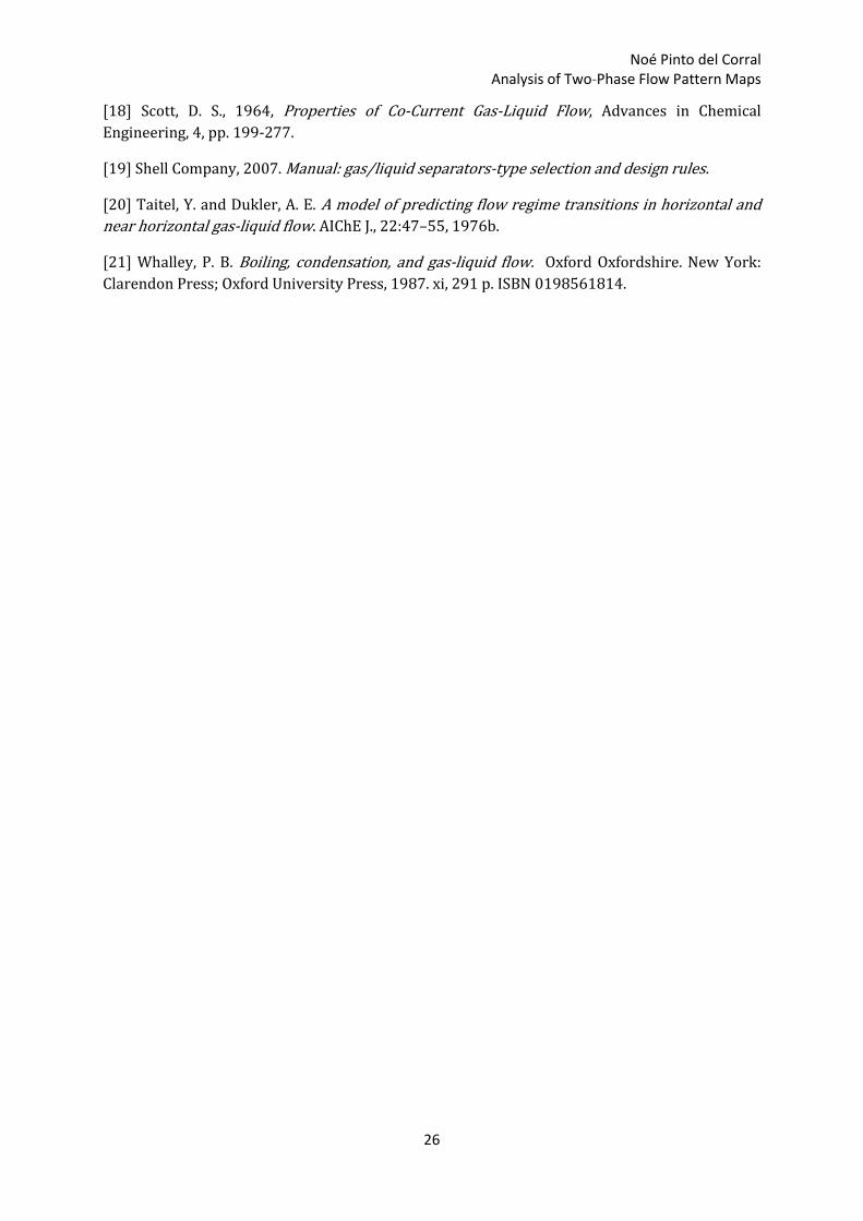
26

[18] Scott, D. S., 1964, Properties of Co-Current Gas-Liquid Flow, Advances in Chemical

Engineering, 4, pp. 199-277.

[19] Shell Company, 2007. Manual: gas/liquid separators-type selection and design rules.

[20] Taitel, Y. and Dukler, A. E. A model of predicting flow regime transitions in horizontal and

near horizontal gas-liquid flow. AIChE J., 22:47–55, 1976b.

[21] Whalley, P. B. Boiling, condensation, and gas-liquid flow. Oxford Oxfordshire. New York:

Clarendon Press; Oxford University Press, 1987. xi, 291 p. ISBN 0198561814.

Documents

Analysis of Two Phase Flow Pattern maps - Energetické · PDF fileDigitized Shell’s DEP 31.22.05.11 map 4.1 Description of the map This map was created by the company Shell ... Analysis