Analysis of time series Riccardo Bellazzi Dipartimento di Informatica e Sistemistica Università di Pavia Italy [email protected]

Analysis of time series

Riccardo BellazziDipartimento di Informatica e

Sistemistica Università di Pavia

[email protected]

0 10 20 30 40 50 60 70150

160

170

180

190

200

210

220

Dialysis sessions

Blo

od

flu

xtime course of blood flux

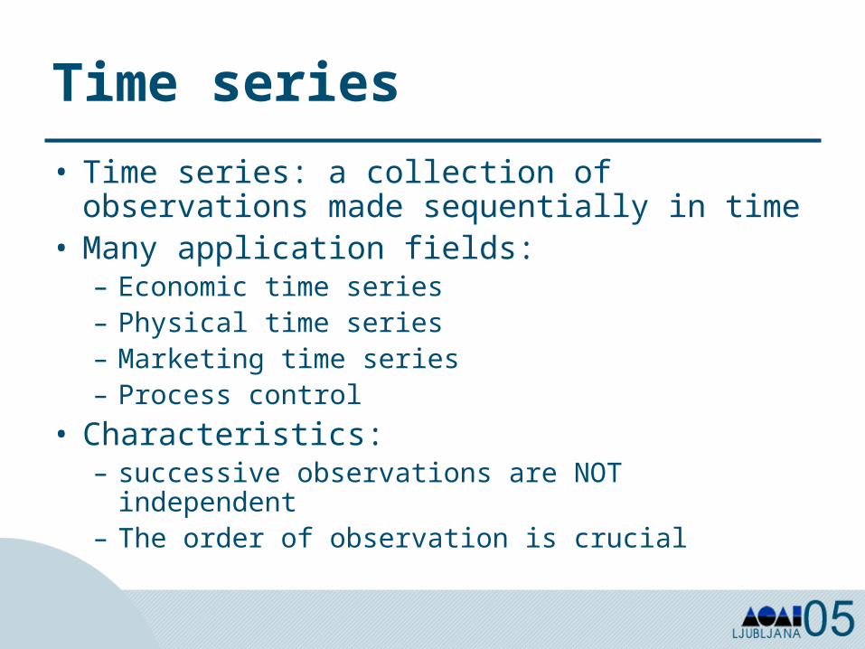
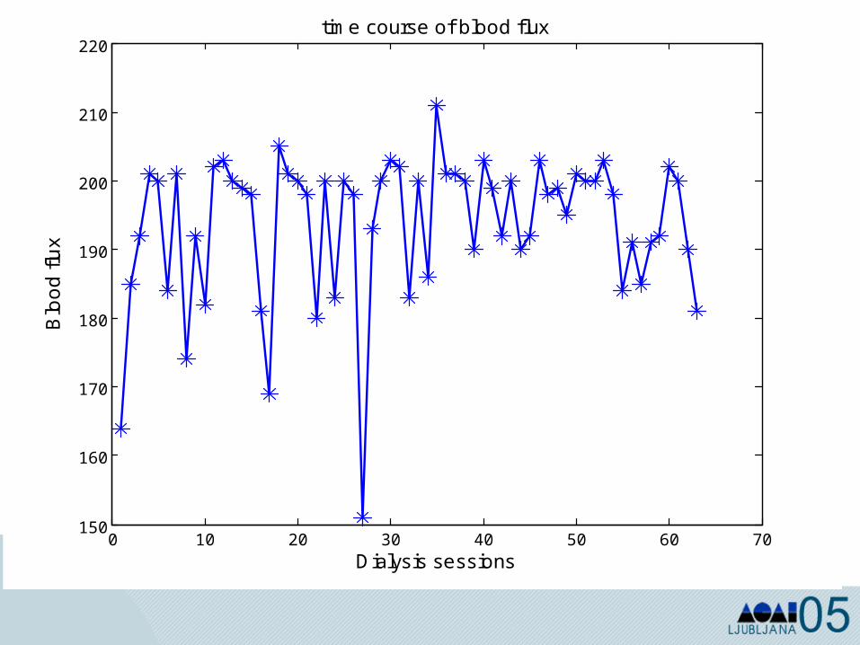
Time series

• Time series: a collection of observations made sequentially in time

• Many application fields:– Economic time series– Physical time series– Marketing time series– Process control

• Characteristics: – successive observations are NOT independent– The order of observation is crucial

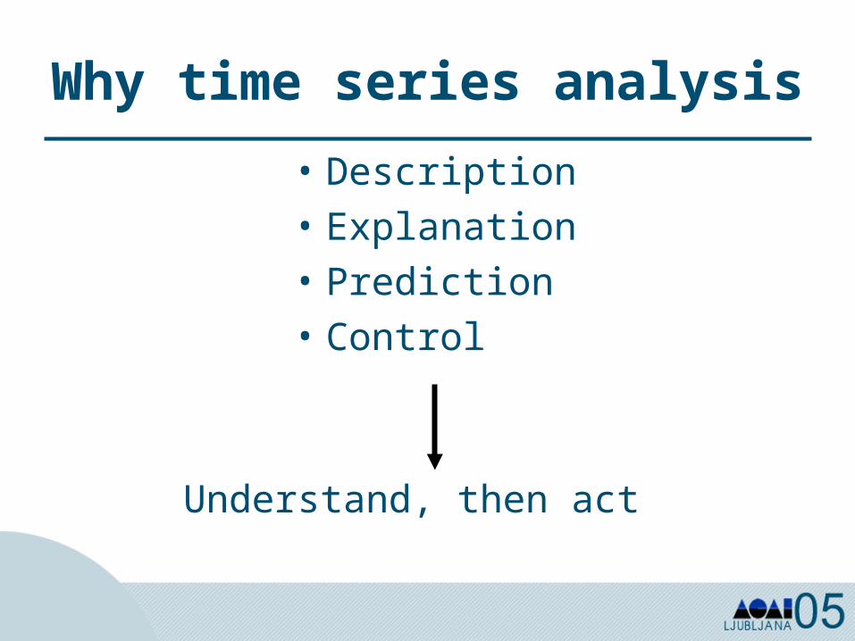
Why time series analysis

• Description• Explanation• Prediction• Control

Understand, then act

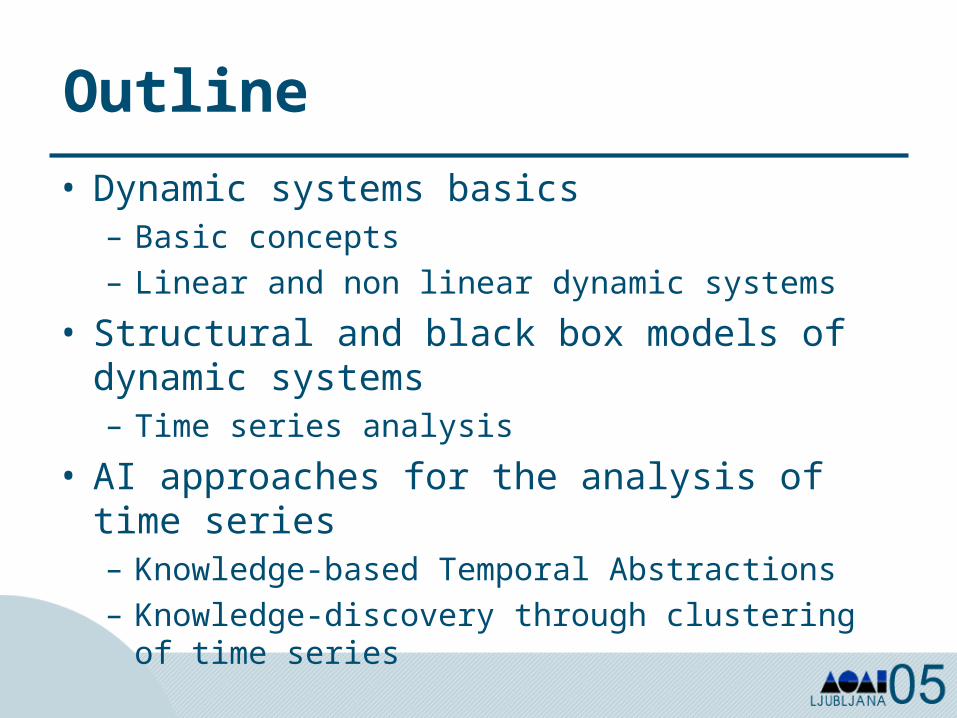
Outline

• Dynamic systems basics– Basic concepts– Linear and non linear dynamic systems

• Structural and black box models of dynamic systems– Time series analysis

• AI approaches for the analysis of time series– Knowledge-based Temporal Abstractions– Knowledge-discovery through clustering of

time series

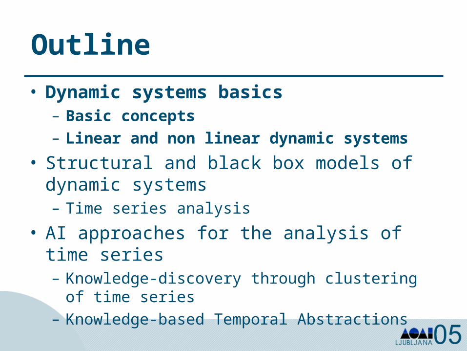
Outline



• AI approaches for the analysis of time series– Knowledge-discovery through clustering of

time series– Knowledge-based Temporal Abstractions

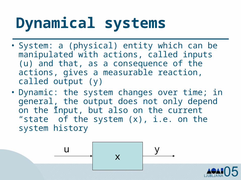
Dynamical systems• System: a (physical) entity which can be

manipulated with actions, called inputs (u) and that, as a consequence of the actions, gives a measurable reaction, called output (y)

• Dynamic: the system changes over time; in general, the output does not only depend on the input, but also on the current “state” of the system (x), i.e. on the system history

xu y

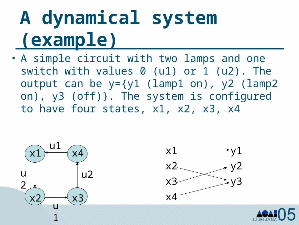
A dynamical system (example)

• A simple circuit with two lamps and one switch with values 0 (u1) or 1 (u2). The output can be y={y1 (lamp1 on), y2 (lamp2 on), y3 (off)}. The system is configured to have four states, x1, x2, x3, x4

x1

x2

x3

x4

y1

y2

y3

x1 x4

x2 x3

u2

u1

u2

u1

Dynamical system definition• A dynamical system is a process in which

a function's value changes over time according to a rule that is defined in terms of the function's current value and the current time.

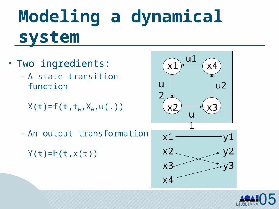
Modeling a dynamical system

• Two ingredients:– A state transition

function

X(t)=f(t,t0,X0,u(.))

– An output transformation

Y(t)=h(t,x(t))

x1

x2

x3

x4

y1

y2

y3

x1 x4

x2 x3

u2

u1

u2

u1

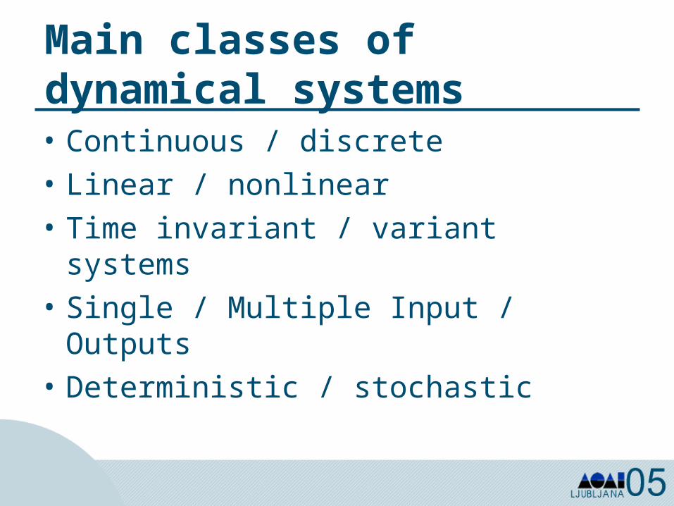
Main classes of dynamical systems• Continuous / discrete• Linear / nonlinear• Time invariant / variant systems• Single / Multiple Input / Outputs• Deterministic / stochastic

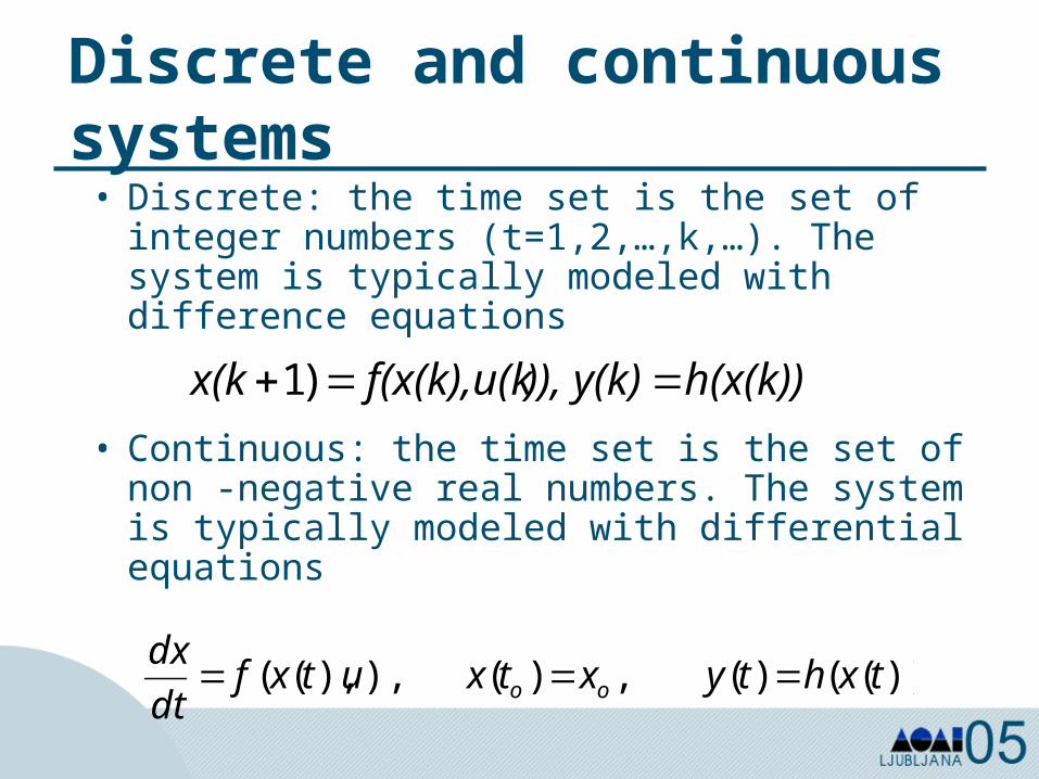
Discrete and continuous systems• Discrete: the time set is the set of integer

numbers (t=1,2,…,k,…). The system is typically modeled with difference equations

• Continuous: the time set is the set of non -negative real numbers. The system is typically modeled with differential equations

))(()(,)(),),(( txhtyxtxutxfdt

dxoo

h(x(k)))), y(k)f(x(k),u(kx(k )1

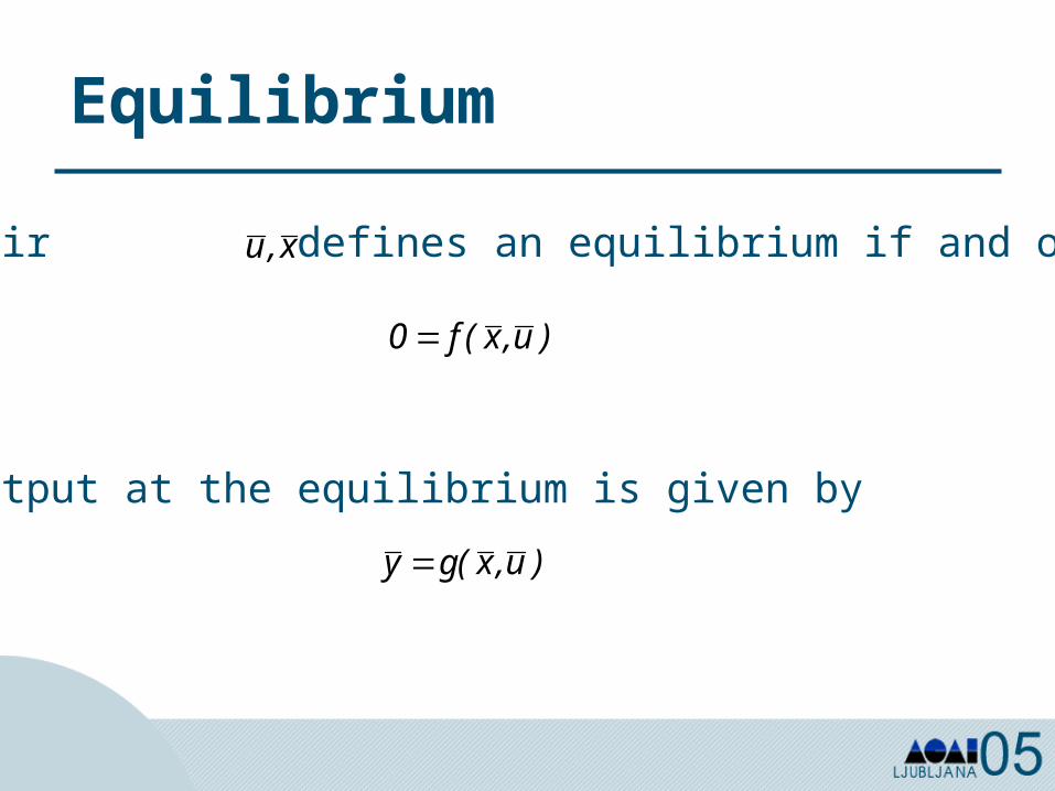
Equilibrium

The pair defines an equilibrium if and only if

The output at the equilibrium is given by

)u,x(gy

x,u

)u,x(f0

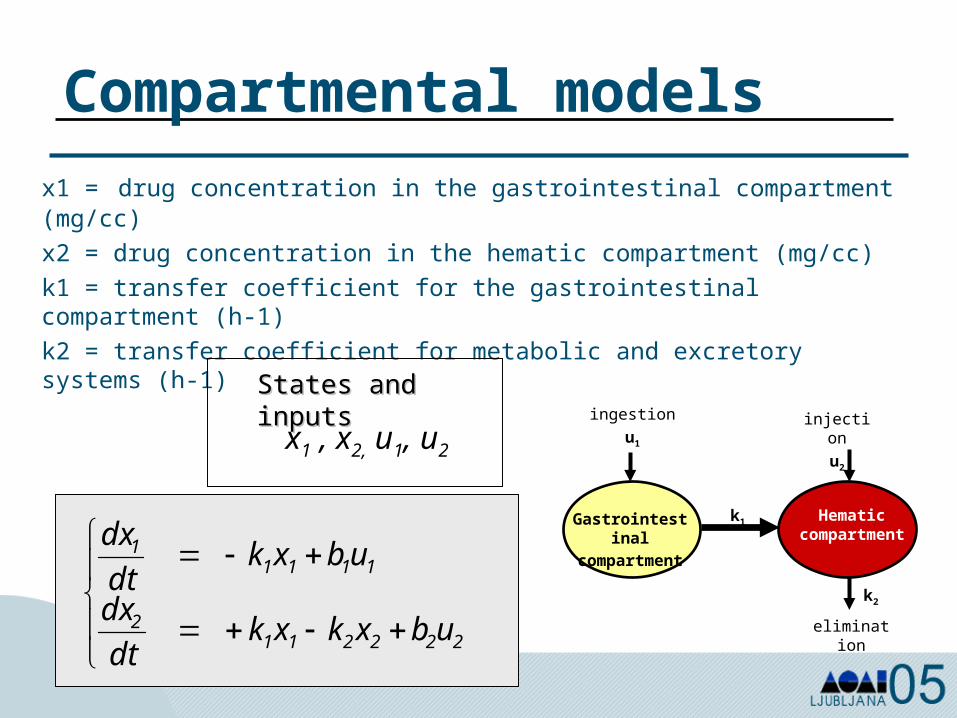
x1 = drug concentration in the gastrointestinal compartment (mg/cc)

x2 = drug concentration in the hematic compartment (mg/cc)k1 = transfer coefficient for the gastrointestinal compartment (h-1)k2 = transfer coefficient for metabolic and excretory systems (h-1)

2222112

11111

ubxkxkdt

dx

ubxkdt

dx

ingestionu1

injectionu2

Gastrointestinal

compartment

Hematiccompartment

k1

elimination

k2

States and States and inputsinputs

x1 , x2, u1, u2

Compartmental models

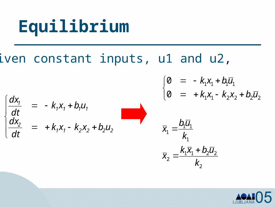
Equilibrium

2

22112

1

111

222211

1111

0

0

k

ubxkx

k

ubx

ubxkxk

ubxk

Given constant inputs, u1 and u2,

2222112

11111

ubxkxkdt

dx

ubxkdt

dx

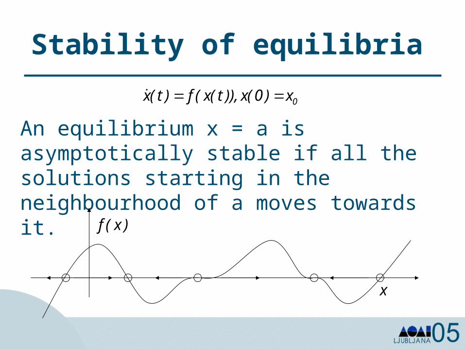
Stability of equilibria

0x)0(x)),t(x(f)t(x

An equilibrium x = a is asymptotically stable if all the solutions starting in the neighbourhood of a moves towards it.

)x(f

x

Stability of trajectories

Stable

Unstable

Asymptotically stable

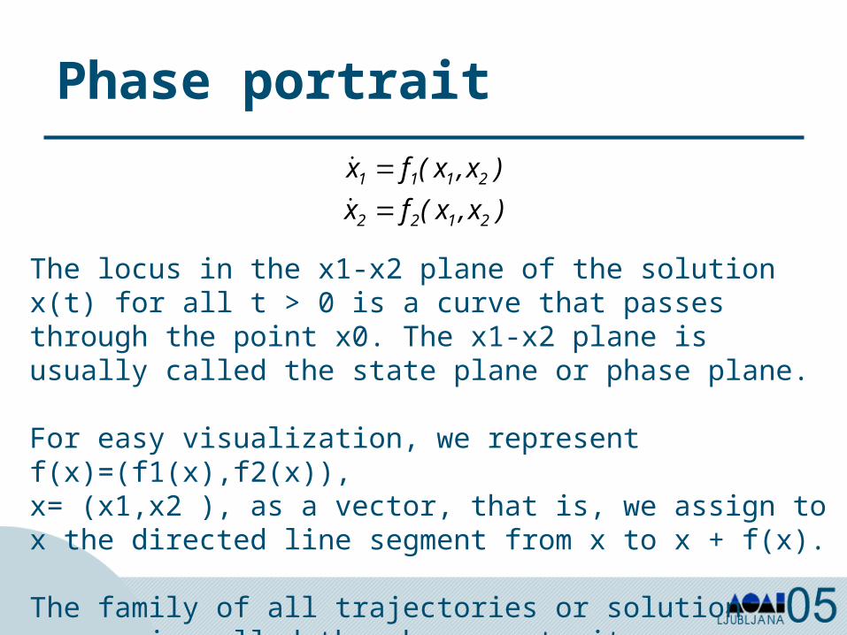
Phase portrait

)x,x(fx

)x,x(fx

2122

2111

The locus in the x1-x2 plane of the solution x(t) for all t > 0 is a curve that passes through the point x0. The x1-x2 plane is usually called the state plane or phase plane.

For easy visualization, we represent f(x)=(f1(x),f2(x)), x= (x1,x2 ), as a vector, that is, we assign to x the directed line segment from x to x + f(x).

The family of all trajectories or solution curves is called the phase portrait.

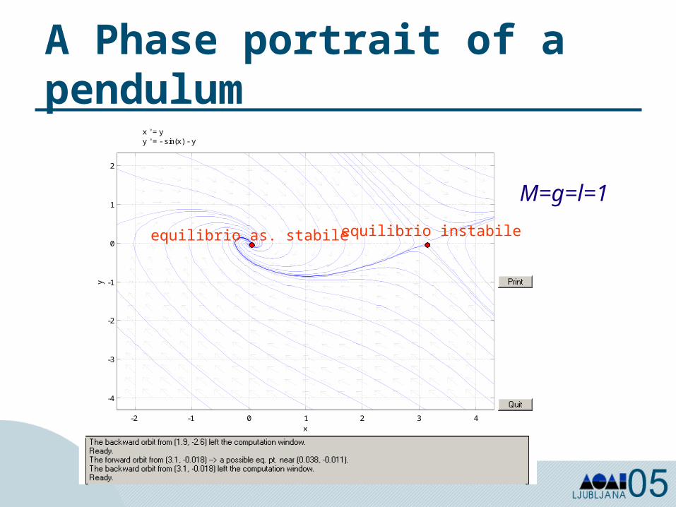
A Phase portrait of a pendulum

x ' = y y ' = - sin(x) - y

-2 -1 0 1 2 3 4

-4

-3

-2

-1

0

1

2

x

y

equilibrio instabileequilibrio as. stabile

M=g=l=1

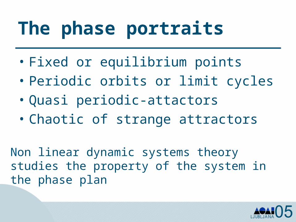
The phase portraits

• Fixed or equilibrium points• Periodic orbits or limit cycles• Quasi periodic-attactors• Chaotic of strange attractors

Non linear dynamic systems theory studies the property of the system in the phase plan

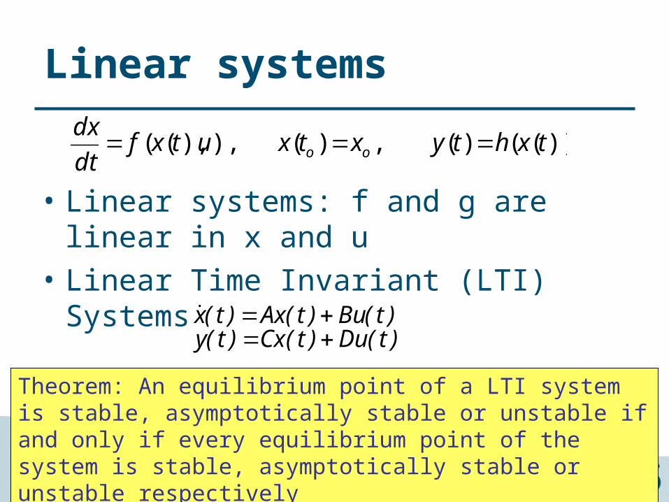
Linear systems

• Linear systems: f and g are linear in x and u

• Linear Time Invariant (LTI) Systems

))(()(,)(),),(( txhtyxtxutxfdt

dxoo

)t(Du)t(Cx)t(y)t(Bu)t(Ax)t(x

Theorem: An equilibrium point of a LTI system is stable, asymptotically stable or unstable if and only if every equilibrium point of the system is stable, asymptotically stable or unstable respectively

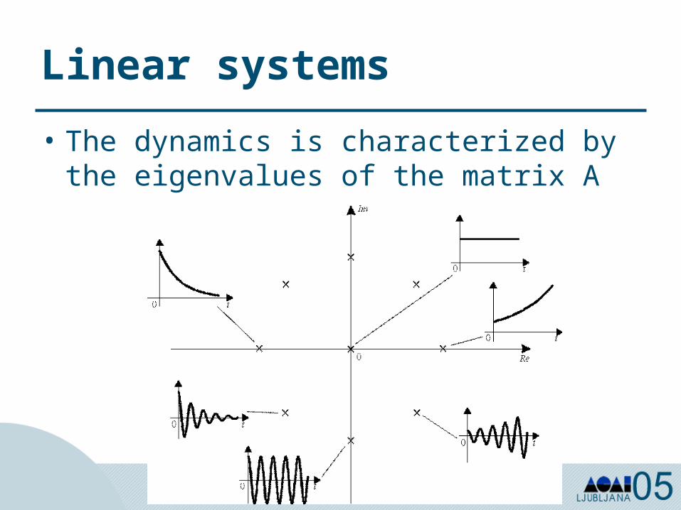
Linear systems

• The dynamics is characterized by the eigenvalues of the matrix A

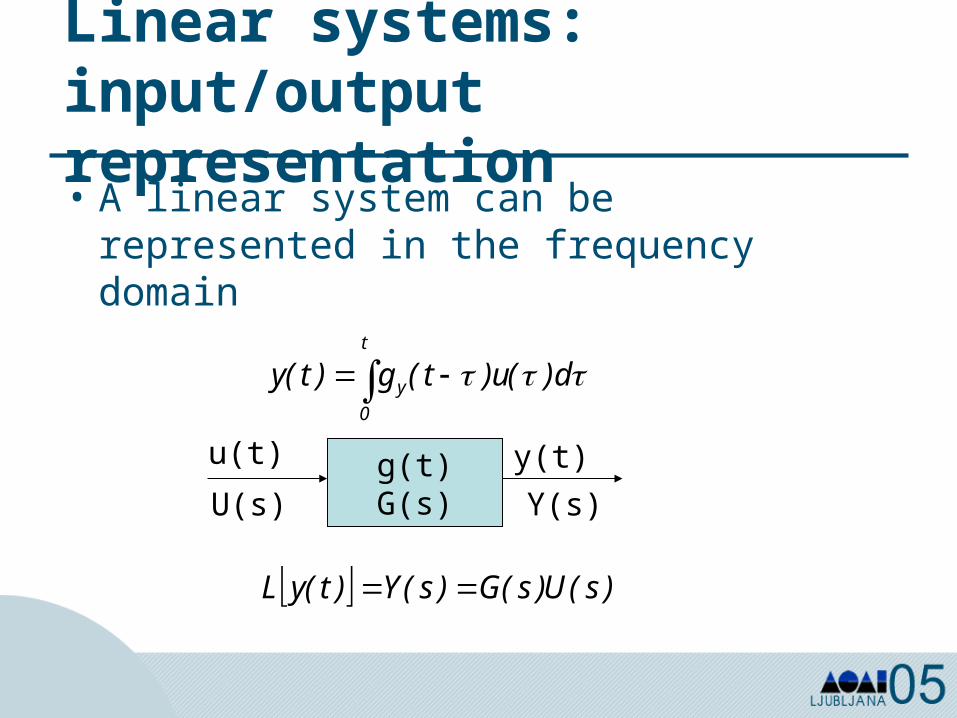
Linear systems: input/output representation• A linear system can be represented

in the frequency domain

t

0

y d)(u)t(g)t(y

)s(U)s(G)s(Y)t(yL

g(t)G(s)

u(t) y(t)

Y(s)U(s)

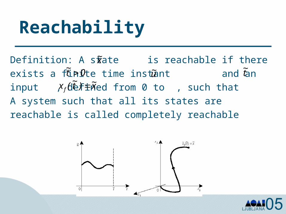
Reachability

Definition: A state is reachable if there exists a finite time instant and an input , defined from 0 to , such thatA system such that all its states are reachable is called completely reachable

x~

0t~ u~ t~

x~)t~(x f

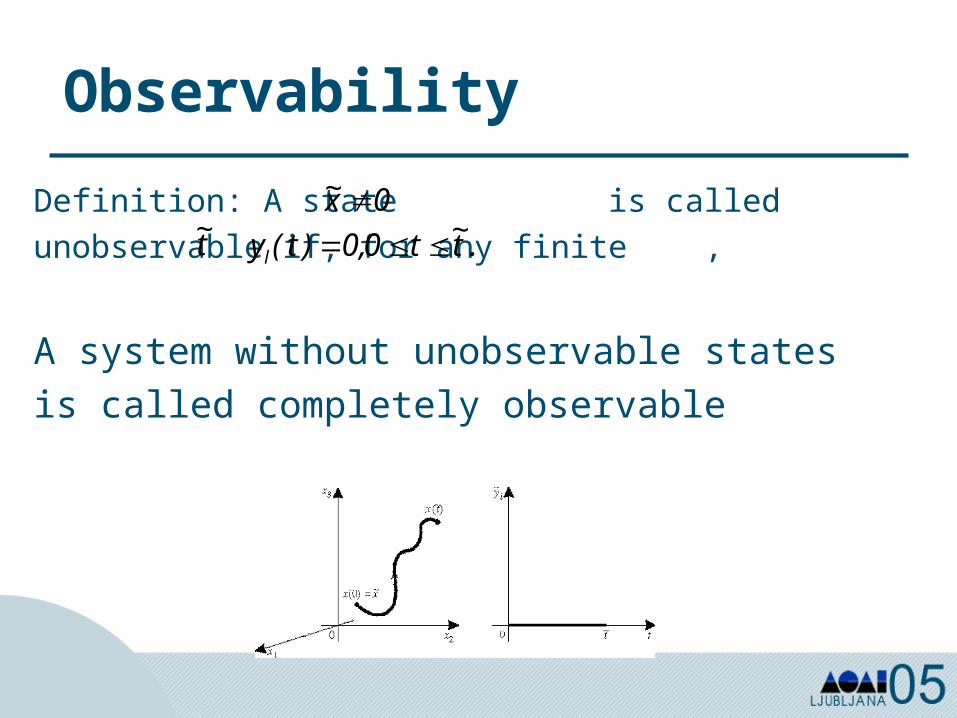
Observability

Definition: A state is called unobservable if, for any finite ,

A system without unobservable states is called completely observable

0x~ .t~t0,0)t(yl t~

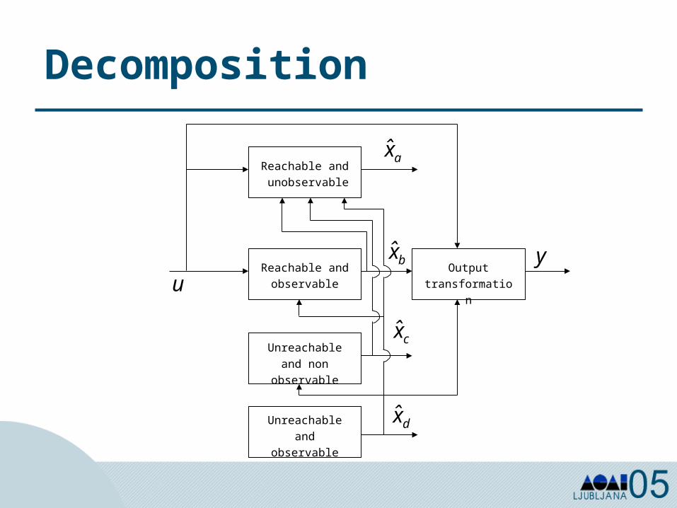
Decomposition

Output transformationu

ax̂

bx̂

cx̂

dx̂

y

Reachable and unobservable

Reachable and observable

Unreachable and non

observable

Unreachable and observable

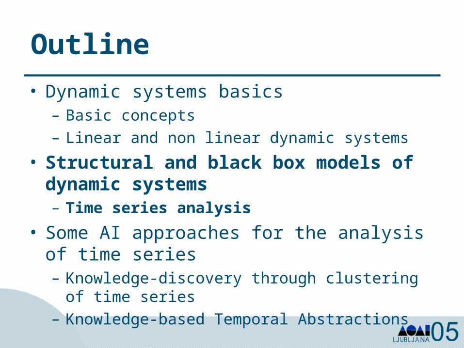
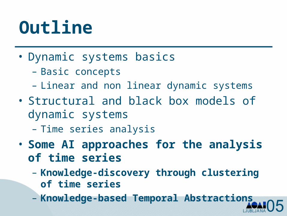
Outline



• Some AI approaches for the analysis of time series– Knowledge-discovery through clustering of


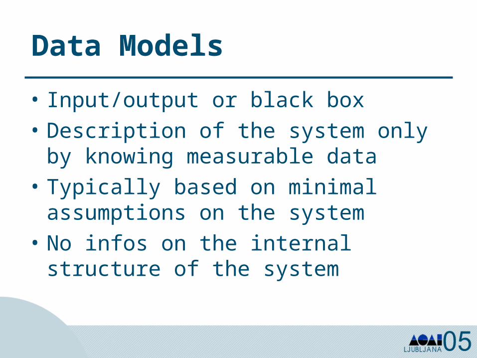
Data Models

• Input/output or black box• Description of the system only by

knowing measurable data• Typically based on minimal

assumptions on the system• No infos on the internal structure of

the system

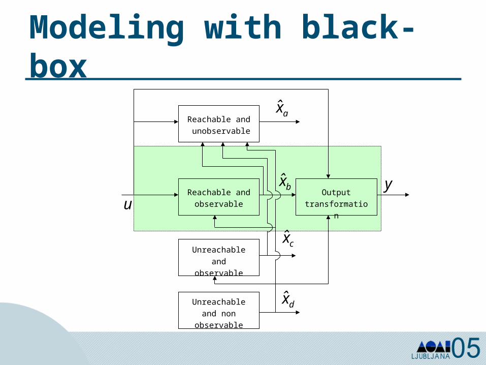
Modeling with black-box


ax̂

bx̂

cx̂

dx̂

y




Unreachable and non

observable

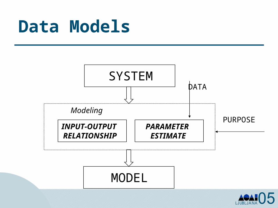
Modeling

MODEL

SYSTEM

INPUT-OUTPUT RELATIONSHIP

PARAMETER ESTIMATE

DATA

PURPOSE

Data Models

Data Models

• Time series• Impulse response• Transfer functions (linear models)• Convolution / deconvolution (linear

models)

0 20 40 60 80 100 120 140 160

0

5

10

15

TEMPOC

ON

CE

NT

RA

ZIO

NE

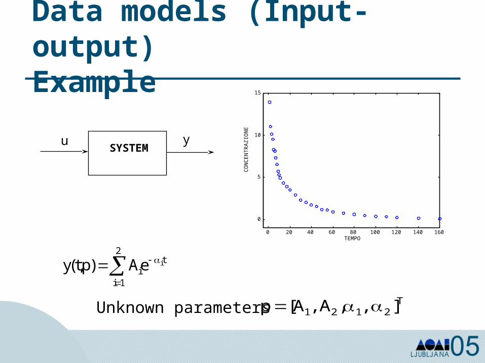
y t p A eit

i

i( , )

1

2

p A T[ , ]1 2 1 2, A ,

SYSTEMu y

Unknown parameters

Data models (Input-output)Example

System Models

• White or grey box• Description of the internal structure

of the system based on physical principles and on explicit hypotesis on causal relationships

• After comparison with experimental data are aimed at understanding the principles of the system

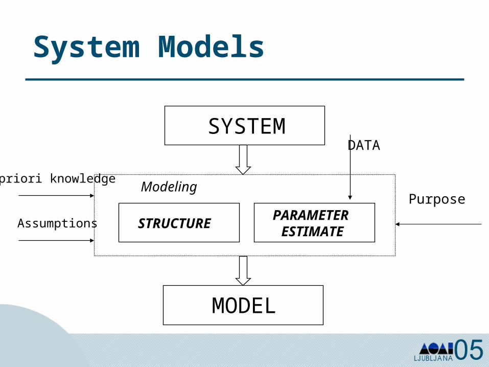
Modeling

MODEL

SYSTEM

STRUCTUREPARAMETER

ESTIMATE

A priori knowledge

Assumptions

DATA

Purpose

System Models

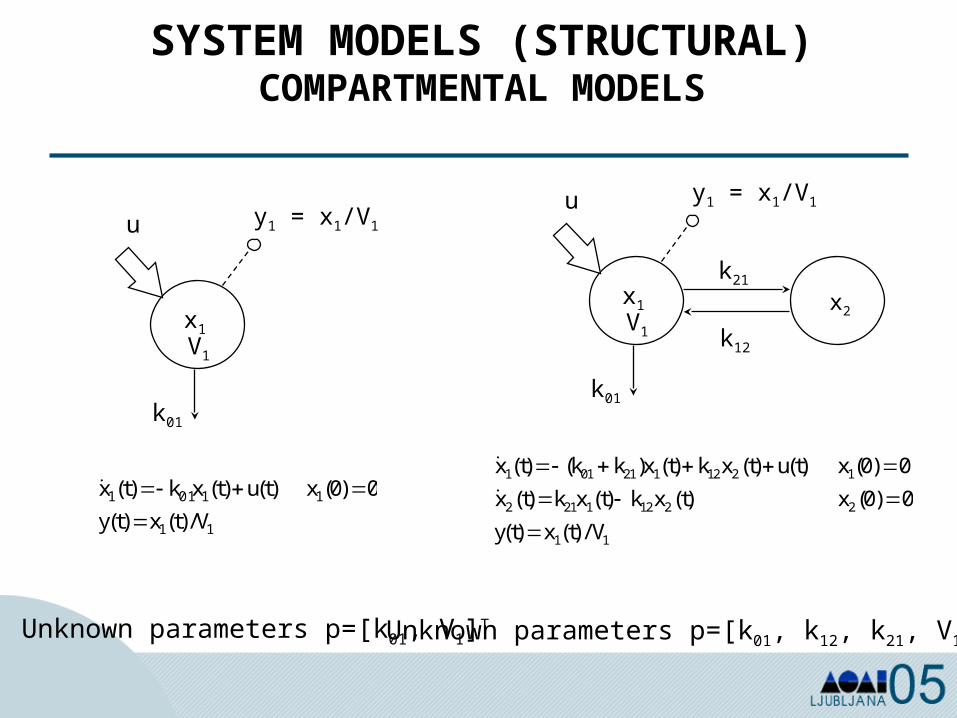
SYSTEM MODELS (STRUCTURAL)COMPARTMENTAL MODELS

Unknown parameters p=[k01, k12, k21, V1]T

( ) ( ) ( ) ( ) ( ) ( ) ( ) ( ) ( ) ( )

( ) ( ) /

x t k k x t k x t u t

x t k x t k x t

y t x t V

1 01 21 1 12 2 1

2 21 1 12 2 2

1 1

0 0

0 0

x

x

x2

k01

k12

k21

y1 = x1/V1u

V1

x1

Unknown parameters p=[k01, V1]T

11

11011

V/)t(x)t(y

0)0(x )t(u)t(xk)t(x

k01

y1 = x1/V1u

V1

x1

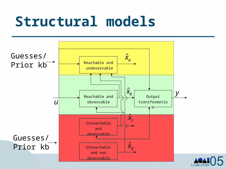
Structural models


ax̂

bx̂

cx̂

dx̂

y




Unreachable and non

observable

Guesses/Prior kb

Guesses/Prior kb

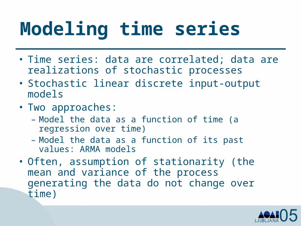
Modeling time series

• Time series: data are correlated; data are realizations of stochastic processes

• Stochastic linear discrete input-output models

• Two approaches:– Model the data as a function of time (a regression

over time)– Model the data as a function of its past values:

ARMA models

• Often, assumption of stationarity (the mean and variance of the process generating the data do not change over time)

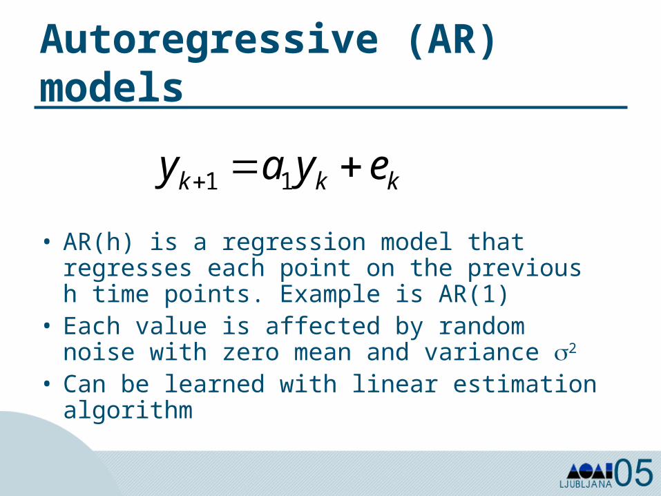
Autoregressive (AR) models

• AR(h) is a regression model that regresses each point on the previous h time points. Example is AR(1)

• Each value is affected by random noise with zero mean and variance 2

• Can be learned with linear estimation algorithm

kkk eyay 11

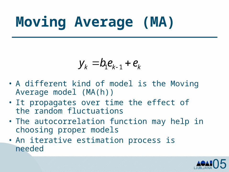
Moving Average (MA)

• A different kind of model is the Moving Average model (MA(h))

• It propagates over time the effect of the random fluctuations

• The autocorrelation function may help in choosing proper models

• An iterative estimation process is needed

kkk eeby 11

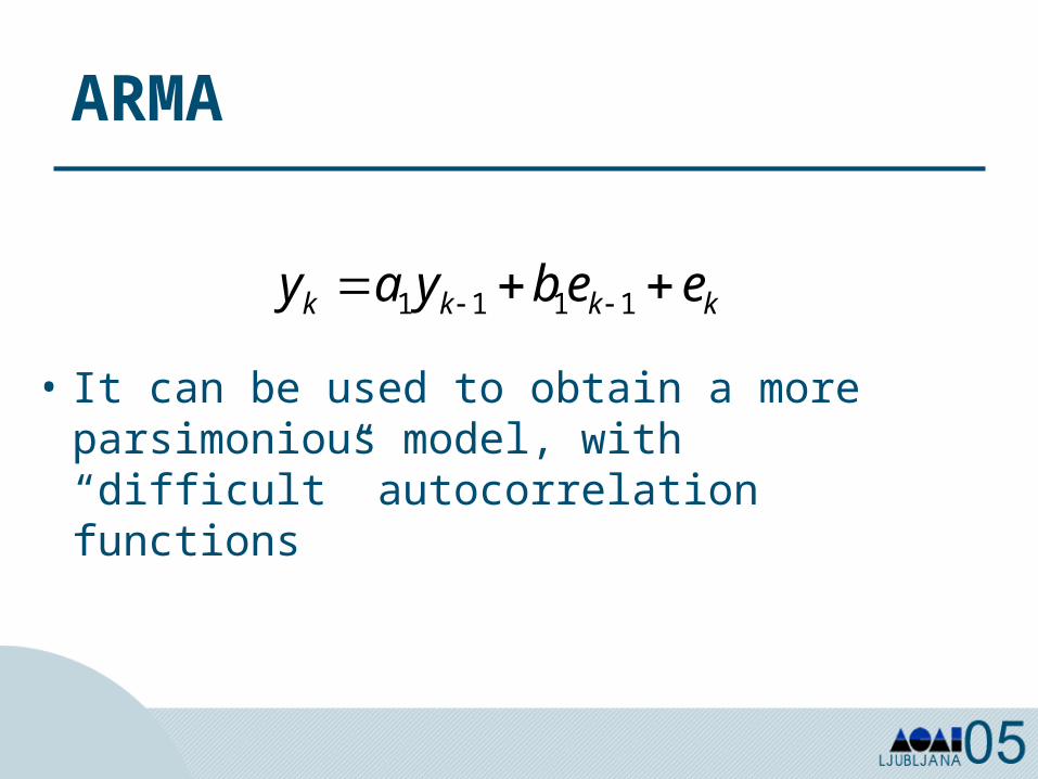
ARMA

• It can be used to obtain a more parsimonious model, with “difficult” autocorrelation functions

kkkk eebyay 1111

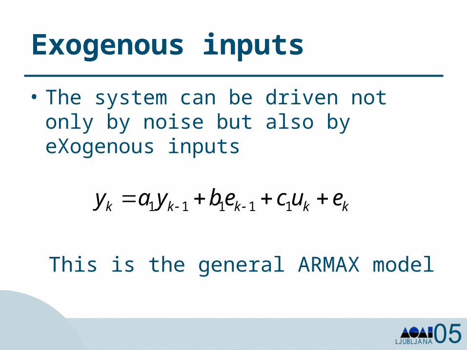
Exogenous inputs

• The system can be driven not only by noise but also by eXogenous inputs

kkkkk eucebyay 11111

This is the general ARMAX model

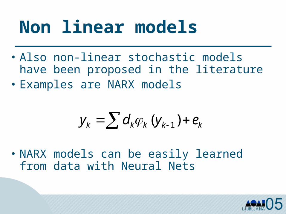
Non linear models

• Also non-linear stochastic models have been proposed in the literature

• Examples are NARX models

• NARX models can be easily learned from data with Neural Nets

kkkkk eydy )( 1

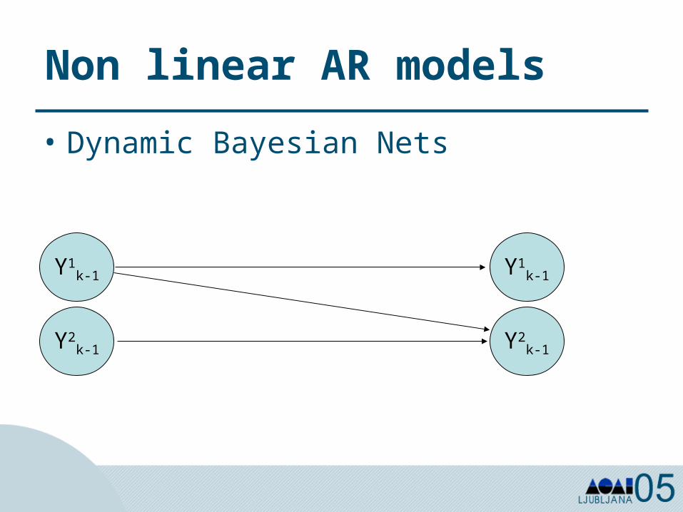
Non linear AR models

• Dynamic Bayesian Nets

Y1k-1

Y2k-1

Y1k-1

Y2k-1

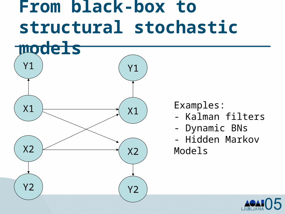
From black-box to structural stochastic models

X1

X2

X1

X2

Y2 Y2

Y1 Y1

Examples:- Kalman filters- Dynamic BNs- Hidden Markov Models

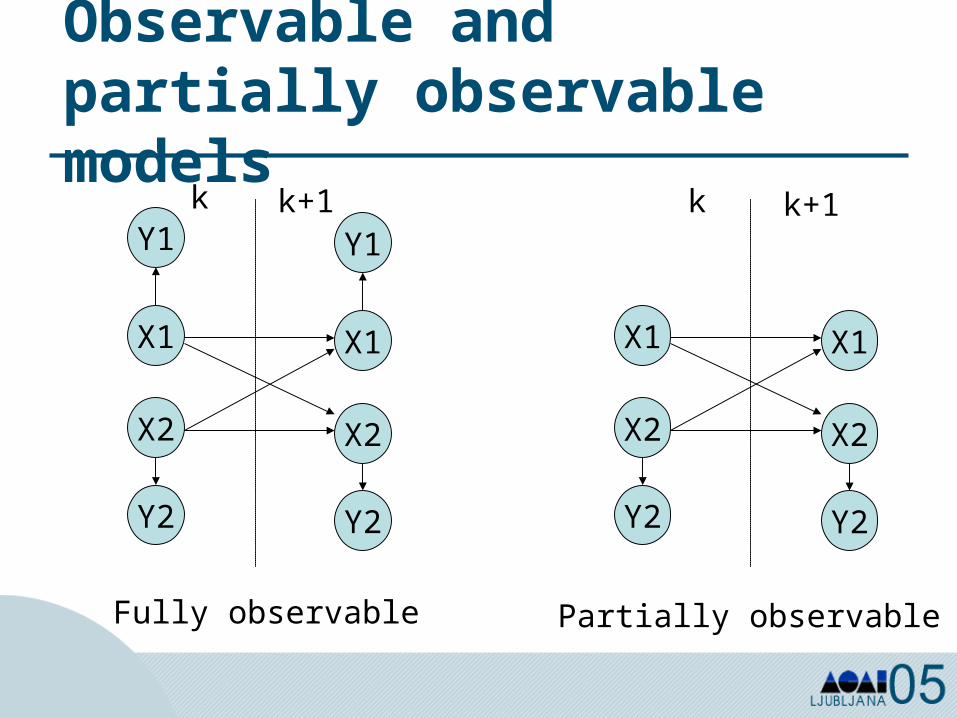
Observable and partially observable models

X1

X2

X1

X2

Y2 Y2

Y1 Y1

Fully observable

X1

X2

X1

X2

Y2 Y2

Partially observable

k k+1 k k+1

Delay coordinate embedding• How to reconstruct a state-space

representation from a uni-dimensional time series y

• Sampled data• Idea: add n state variables using the

values of y with a delay of tau

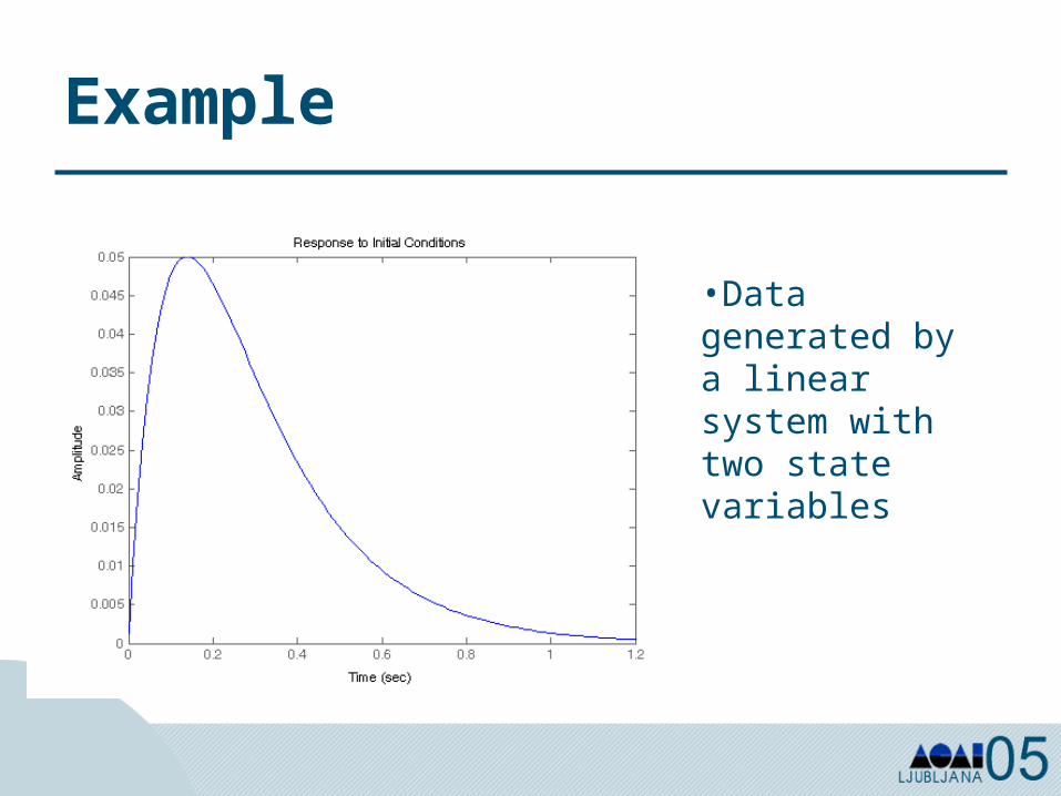
Example

•Data generated by a linear system with two state variables

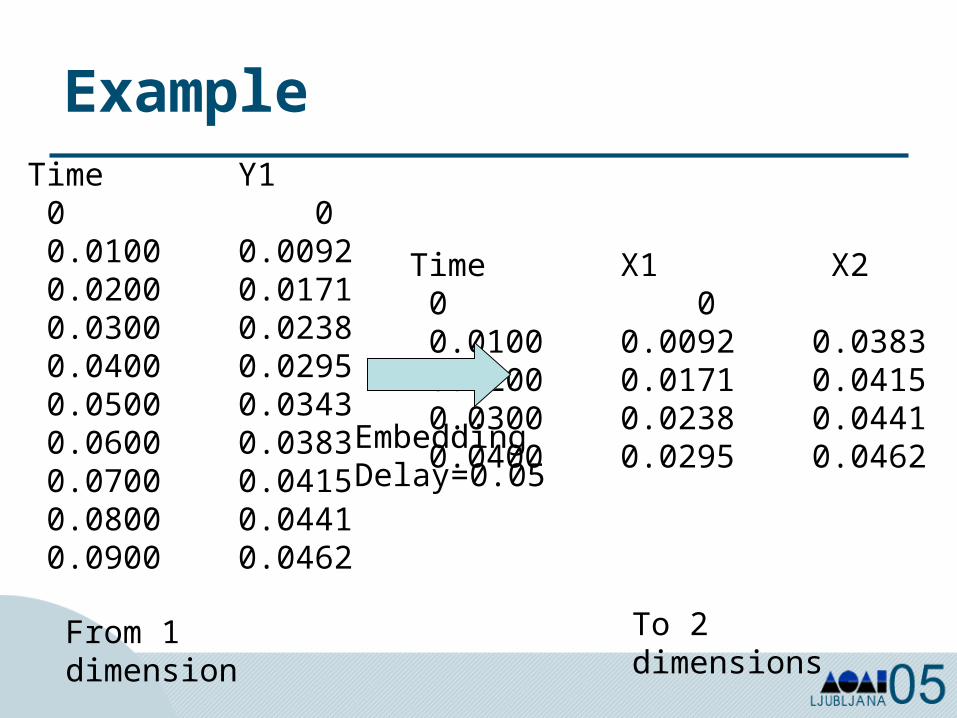
Example Time Y1 0 0 0.0100 0.0092 0.0200 0.0171 0.0300 0.0238 0.0400 0.0295 0.0500 0.0343 0.0600 0.0383 0.0700 0.0415 0.0800 0.0441 0.0900 0.0462

From 1 dimension

Time X1 X2 0 0 0.0343 0.0100 0.0092 0.0383 0.0200 0.0171 0.0415 0.0300 0.0238 0.0441 0.0400 0.0295 0.0462

To 2 dimensions

EmbeddingDelay=0.05

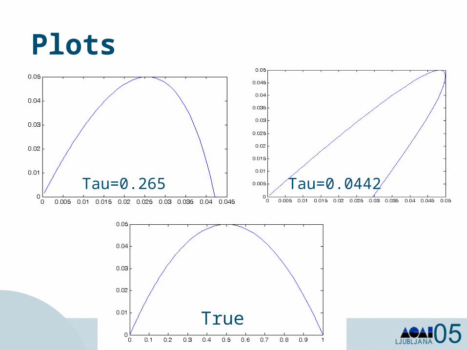
Plots

True

Tau=0.265 Tau=0.0442

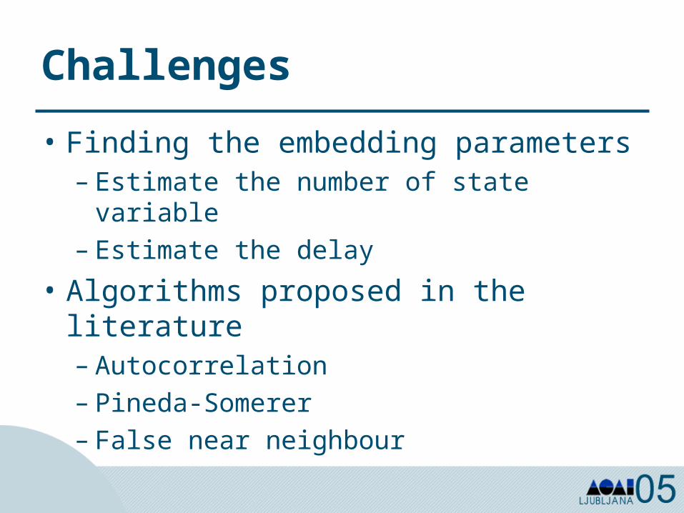
Challenges

• Finding the embedding parameters– Estimate the number of state variable– Estimate the delay

• Algorithms proposed in the literature– Autocorrelation– Pineda-Somerer– False near neighbour

Outline



• Some AI approaches for the analysis of time series– Knowledge-discovery through clustering

of time series– Knowledge-based Temporal Abstractions

Clustering of time series

Several methodologies available

• Similarity-based clustering

• Model-based clustering

• Template-based clustering

Zhong, S., Ghosh, J., Journal of Machine Learning Research, 2003


Several methodologies available





Similarity-Based Clustering

Key point: to define a distance measure (similarity function) between time series.

Strategy: temporal profiles which verify the same similarity condition are grouped together.

Different classes of algorithms: hierarchical clustering, partitioning methods, self-organizing maps.

Eisen et al., 1998; Tamayo et al., 1999

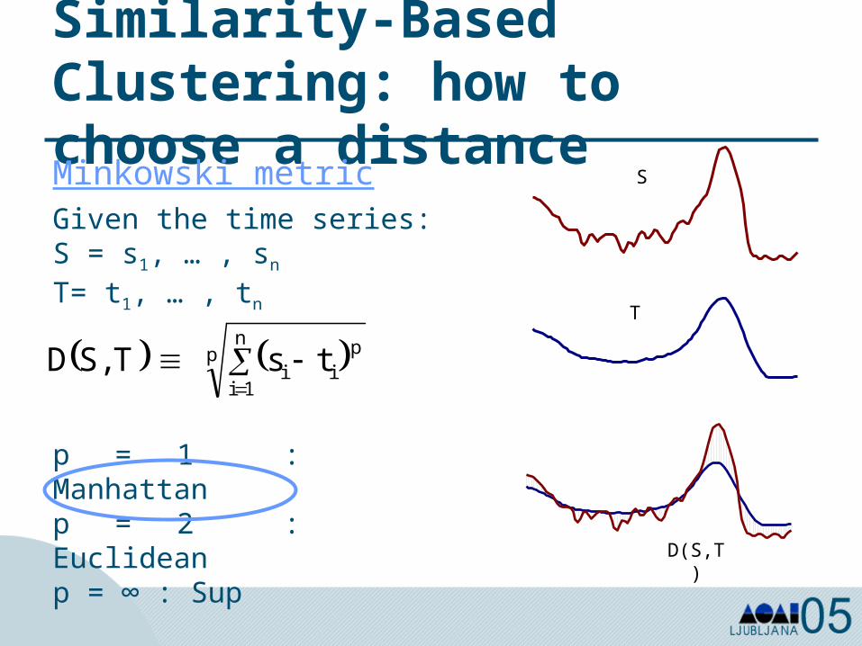
Similarity-Based Clustering: how to choose a distance

pn

1i

pii tsTS,D

Minkowski metricGiven the time series:S = s1, … , sn

T= t1, … , tn

S

T

D(S,T)

p = 1 : Manhattanp = 2 : Euclideanp = ∞ : Sup

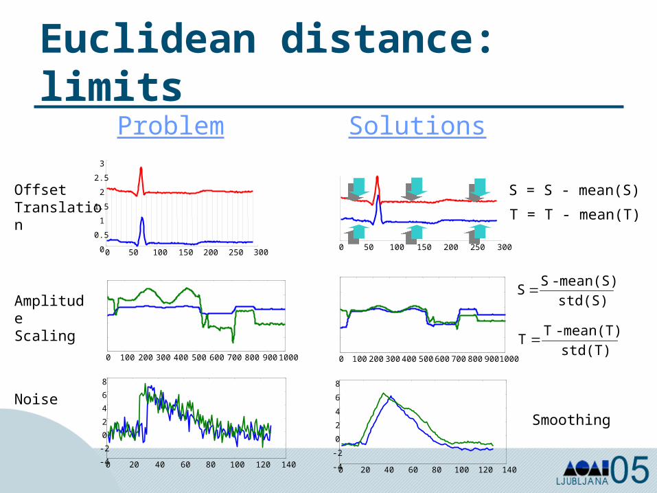
Euclidean distance: limits

0 50 100 150 200 250 3000

0.5

1

1.5

2

2.5

3

0 100 200 300 400 500 600 700 800 900 1000

0 20 40 60 80 100 120 140-4

-2

0

2

4

6

8

0 50 100 150 200 250 300

Offset Translation

Amplitude Scaling

Noise

S = S - mean(S)

T = T - mean(T)

0 100 200 300 400 500 600 700 800 900 1000

std(S)mean(S) - S

S

std(T)mean(T) - T

T

0 20 40 60 80 100 120 140-4

-2

0

2

4

6

8

Smoothing

Problem Solutions

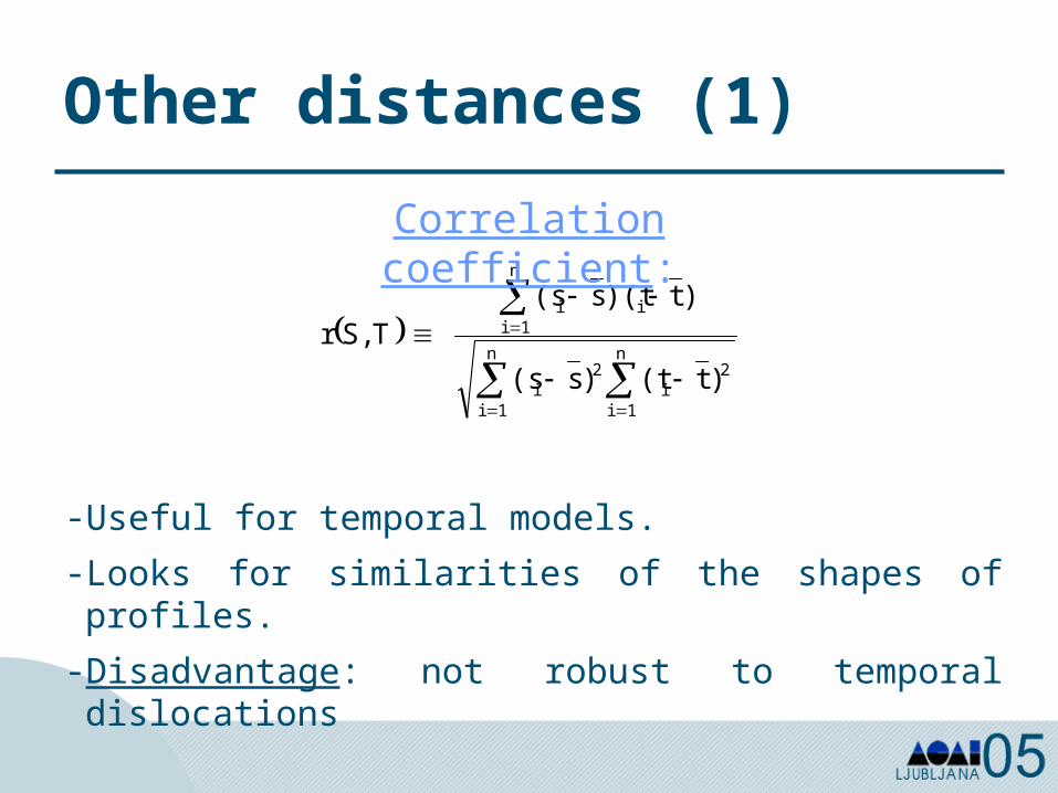
Other distances (1)

n

1 i

n

1 i

2i

2i

n

1 iii

)t (t)s (s

)t)(ts (sTS,r

Correlation coefficient:

- Useful for temporal models.

- Looks for similarities of the shapes of profiles.

- Disadvantage: not robust to temporal dislocations

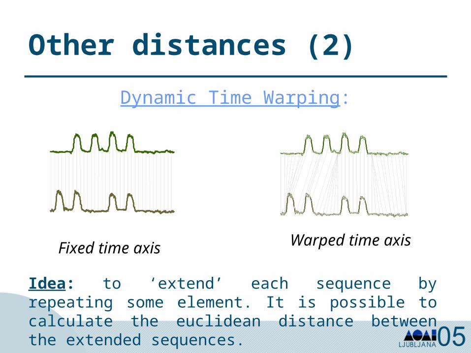
Other distances (2)

Dynamic Time Warping:

Fixed time axis Warped time axis

Idea: to ‘extend’ each sequence by repeating some element. It is possible to calculate the euclidean distance between the extended sequences.

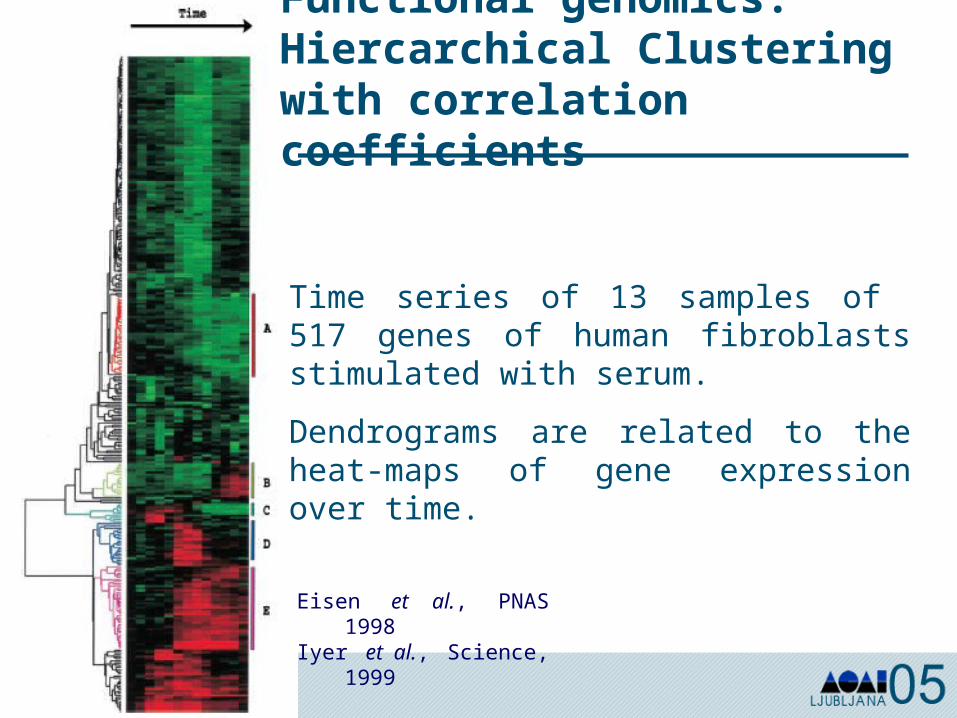
Functional genomics: Hiercarchical Clustering with correlation coefficients

Time series of 13 samples of 517 genes of human fibroblasts stimulated with serum.

Dendrograms are related to the heat-maps of gene expression over time.

Eisen et al., PNAS 1998Iyer et al., Science,

1999






Model-based Clustering (1)

Key point: assume that the data are sampled from a population composed by sub-populations characterized by different stochastic processes;

clusters + processes = model

Strategy: the temporal profiles generated by the same stochastic process are grouped in the same cluster. The clustering problem becomes a problem of model selection.

Cheesman and Stutz, 1996; Fraley and Raftery, 2002; Yeung et al., 2001

Model-based Clustering (2)

Given:Y : the dataM: a set of stochastic dynamic models and a cluster division

Θ: the model parameters

A suitable approach:- Bayesian approach: select the model which maximize the posterior probability of the model M given the data Y, P(M|Y)

Ramoni e Sebastiani, 1999; Baldi e Brunak, 1998; Kay, 1993

The Bayesian SolutionRamoni et al., PNAS 2002

Analysis of gene expression time series: CAGED system (Cluster Analysis of Gene Expression Dynamics)

Assumption: time series generated by an unknown number of autoregressive stochastic processes (AR)

From Bayes theorem: P(M|Y) proportional to f(Y|M) (marginal likelihood)

Assumption + hypothesis on the distribution on the model parameters calculation of f(Y|M) for each possible model in closed form

Model selection: agglomerative process + heuristic strategy

Cluster number: automatically selected maximizing the marginal likelihood






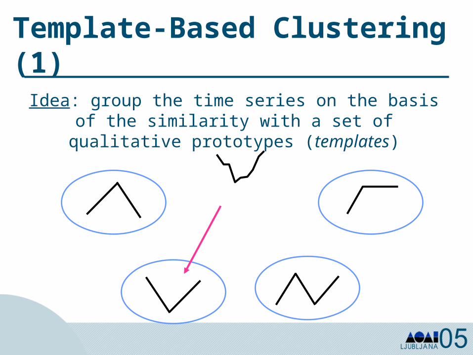
Template-Based Clustering (1)Idea: group the time series on the basis of the similarity with a

set of qualitative prototypes (templates)

Template-Based Clustering (2)

Data representation: from quantitative to qualitative

Templates may capture the relevant characteristics of an expression profile, although they can eliminate the spurious effects caused by noise.

They may simplify the process of capturing the variety of behavior which characterize the gene expression profiles.

Current Limit: templates and clusters have to be a-priori identified.

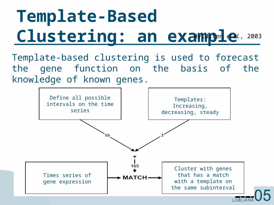
Template-Based Clustering: an example Hvidsten et al., 2003

Template-based clustering is used to forecast the gene function on the basis of the knowledge of known genes.

Define all possible intervals on the time

series

Templates: Increasing, decreasing, steady

Times series of gene expression

Cluster with genes that has a match with a

template on the same subinterval

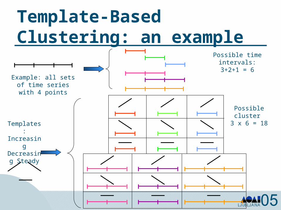
Template-Based Clustering: an example

Example: all sets of time series with 4

points

Templates: Increasing Decreasing

Steady

Possible time intervals: 3+2+1

= 6

Possible cluster 3 x 6 = 18

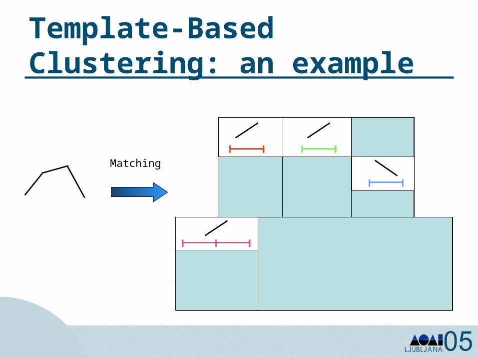
Template-Based Clustering: an example

Matching

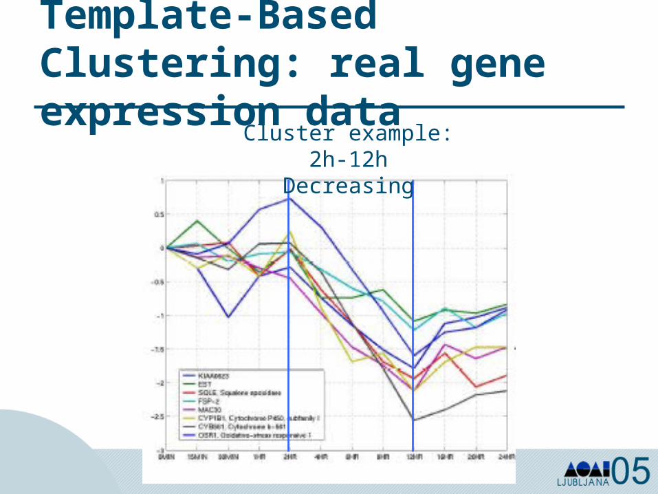
Template-Based Clustering: real gene expression data

Cluster example: 2h-12h Decreasing

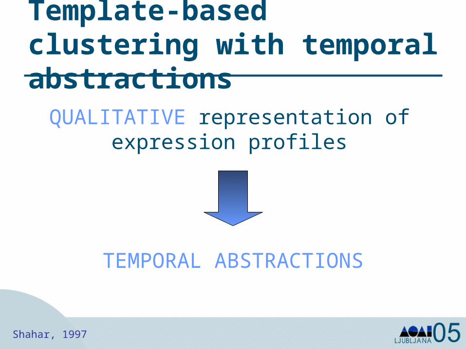
Template-based clustering with temporal abstractions

QUALITATIVE representation of expression profiles

TEMPORAL ABSTRACTIONS

Shahar, 1997

Temporal Primitives

• Time point

• Interval

Temporal Entities

• Events (<time-point, value>)

• Episodes (<interval, pattern>)

Pattern: specific data course (decreasing, normal, stationary, …)

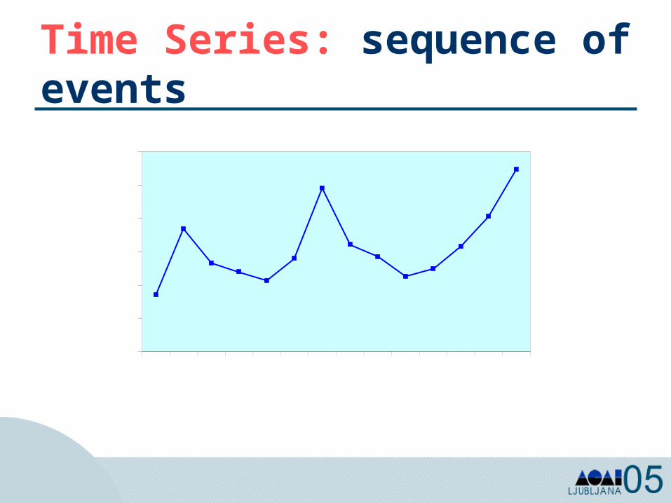
Time Series: sequence of events

0

50

100

150

200

250

300

1 2 3 4 5 6 7 8 9 10 11 12 13 14Time (days)

BG

L (

U/m

l)

Data Abstraction Methods• Qualitative Abstraction: quantitative

data are abstracted into qualitative (a BGL of 110 U/ml is abstracted into normal value)

• Temporal Abstraction (TA): time stamped data are aggregated into intervals associated to specific patterns.

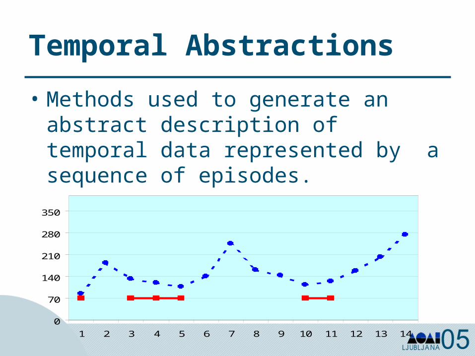
Temporal Abstractions

• Methods used to generate an abstract description of temporal data represented by a sequence of episodes.

0

70

140

210

280

350

1 2 3 4 5 6 7 8 9 10 11 12 13 14

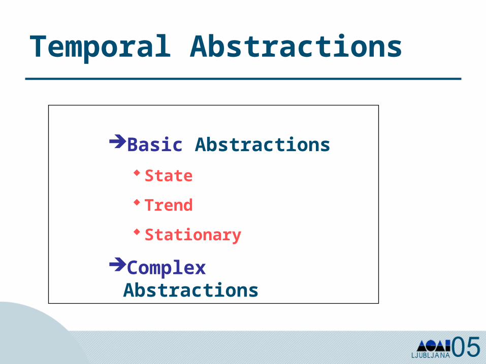
Temporal Abstractions

Basic AbstractionsState

Trend

Stationary

Complex Abstractions

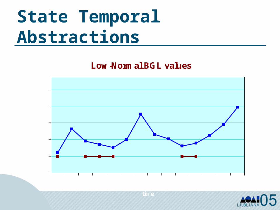
State Temporal Abstractions

Low-Normal BGL values

0

70

140

210

280

350

1 2 3 4 5 6 7 8 9 10 11 12 13 14time

BG

L (

U/m

l)

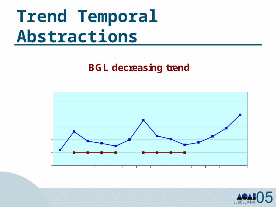
Trend Temporal Abstractions

BGL decreasing trend

0

70

140

210

280

350

1 2 3 4 5 6 7 8 9 10 11 12 13 14Time (days)

BG

L (

U/m

l)

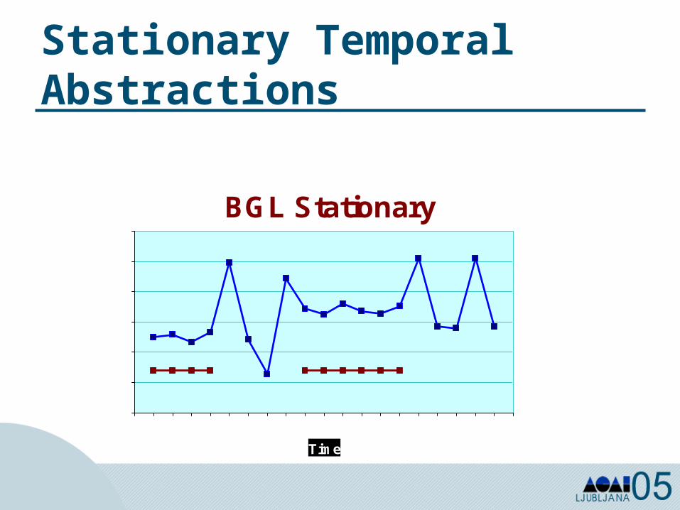
Stationary Temporal Abstractions

BGL Stationary

0

50

100

150

200

250

300

0 1 2 3 4 5 6 7 8 9 10 11 12 13 14 15 16 17 18 19 20

Time

BG

L (

U/m

l)

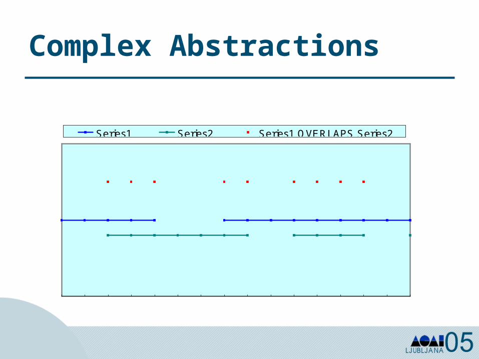
Complex Abstractions

1 2 3 4 5 6 7 8 9 10 11 12 13 14 15 16

Time

Series1 Series2 Series1 OVERLAPS Series2

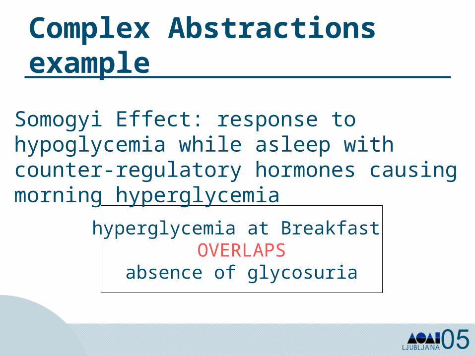
Complex Abstractionsexample

hyperglycemia at Breakfast OVERLAPS

absence of glycosuria

Somogyi Effect: response to hypoglycemia while asleep with counter-regulatory hormones causing morning hyperglycemia

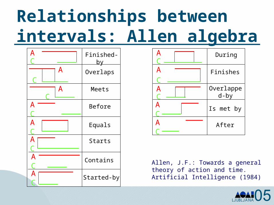
Relationships between intervals: Allen algebra

Finished-by

Overlaps

Meets

Before

Equals

Starts

AC

AC

AC

ACACACAC

Contains

Started-byAC

During

Finishes

Overlapped-by

Is met by

After

ACACACACAC

Allen, J.F.: Towards a general theory of action and time. Artificial Intelligence (1984)

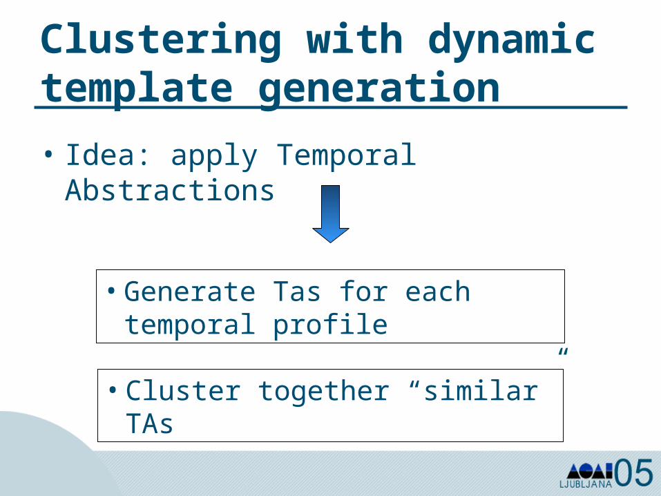
Clustering with dynamic template generation

• Idea: apply Temporal Abstractions

• Generate Tas for each temporal profile

• Cluster together “similar” TAs

Time

Expression

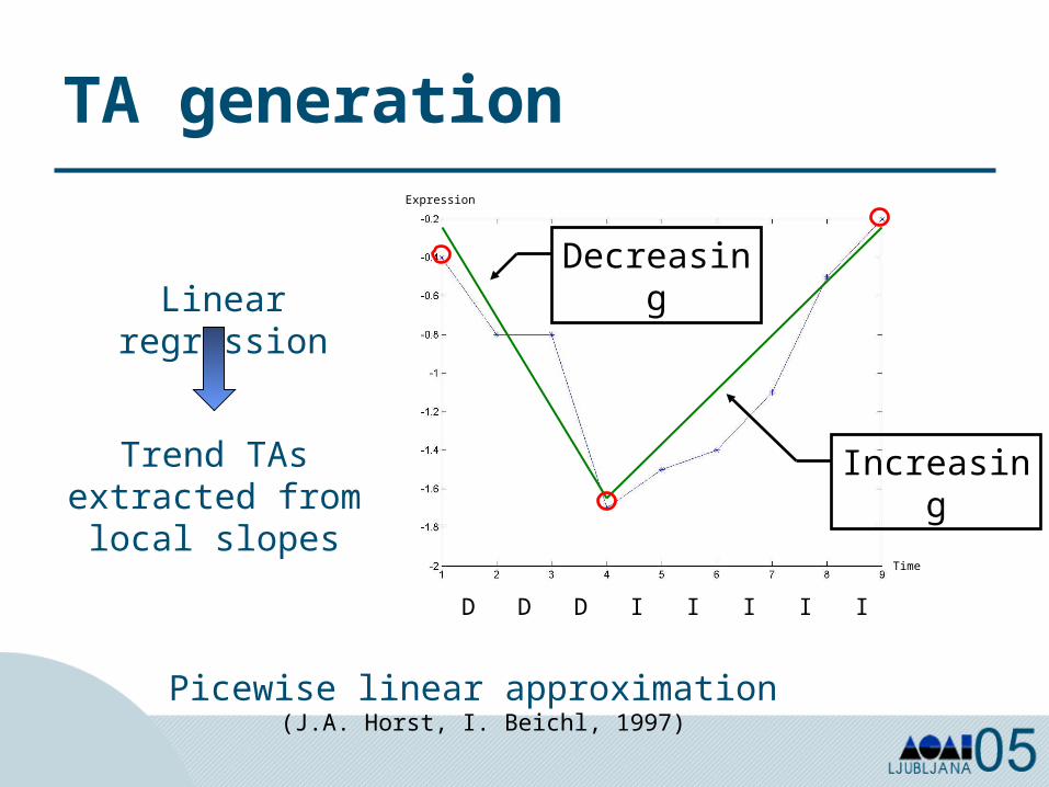
TA generation

Picewise linear approximation (J.A. Horst, I. Beichl, 1997)

D D D I II I I

Decreasing

Increasing

Original time series

Dominant points detection

Threshold needed

Linear regression

Trend TAs extracted from local

slopes

I S I

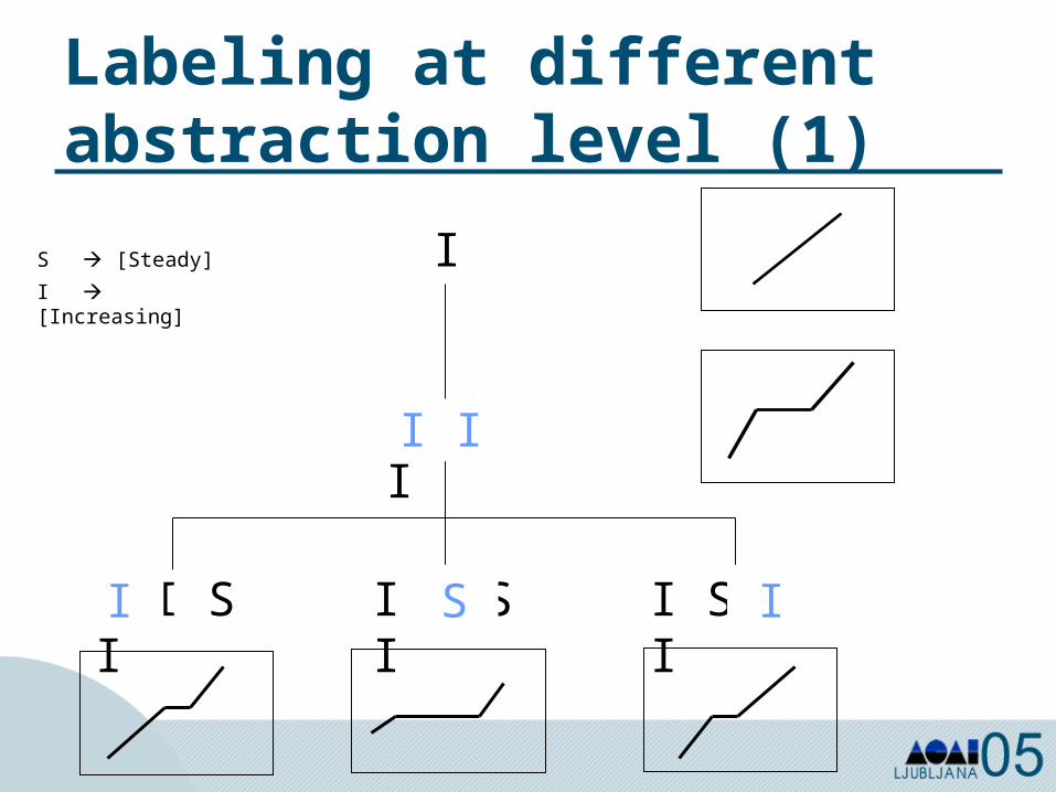
Labeling at different abstraction level (1)

S [Steady]

I [Increasing]

I I S I I S S I I S I II S I

I I

I

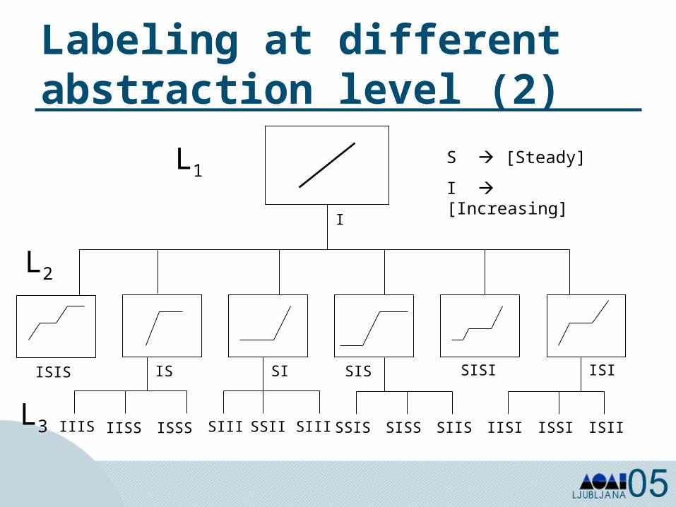
Labeling at different abstraction level (2)

IISSIIIS ISSS SIII SSII SIII SSIS SISS SIIS

S [Steady]

I [Increasing]

IISI ISSI ISII

ISIS IS SI SIS SISI ISI

I

L1

L2

L3

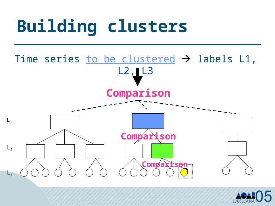
Building clusters

Time series to be clustered labels L1, L2, L3

L1

L2

L3 ?

Comparison

Comparison

Comparison

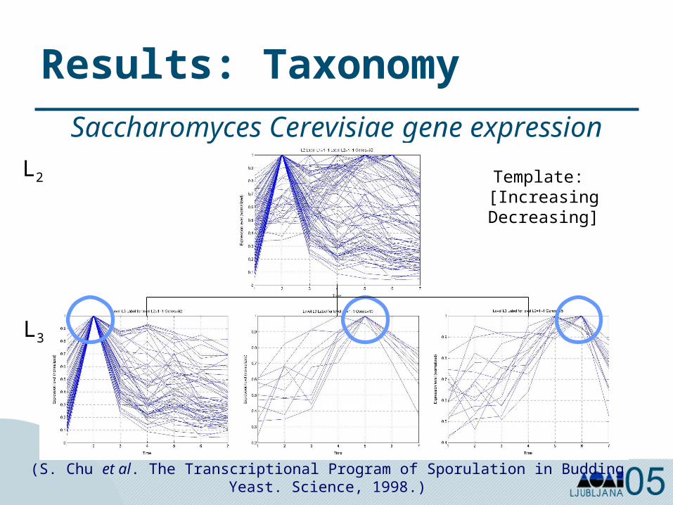
Results: TaxonomySaccharomyces Cerevisiae gene expression

L3

L2

(S. Chu et al. The Transcriptional Program of Sporulation in Budding Yeast. Science, 1998.)

Template: [Increasing Decreasing]

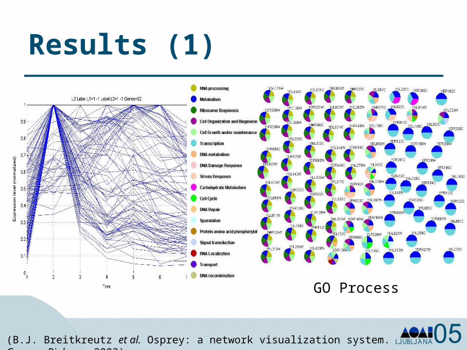
Results (1)

GO Process

(B.J. Breitkreutz et al. Osprey: a network visualization system. Genome Biology, 2003)

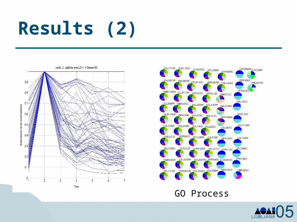
Results (2)

GO Process

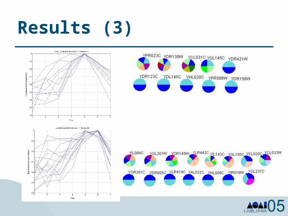
Results (3)

Outline



• AI approaches for the analysis of time series– Knowledge-discovery through clustering of


Conclusions

• Time is a (the?) crucial aspect of our lives

• It is therefore crucial for Intelligent data analysis

• Understanding the dynamics of processes through modeling

• IDA as an interdisciplinary field manage time by combining systems theory, probability theory, AI, …

Documents

Analysis of time series Riccardo Bellazzi Dipartimento di Informatica e Sistemistica Università di Pavia Italy [email protected]