Analysis of the tool for the valuation of R&D projectsessay.utwente.nl/58103/1/scriptie_W_Chung.pdf · · 2011-08-28Analysis of the tool for the valuation of R&D projects ... This

Analysis of the tool for the valuation of R&D projects A research conducted by Philips Lighting

Author: Willem Chung

Student number: s0025267

Educational Institution: University Twente

Company: Philips Lighting

Supervisor at the company: Ruud Gal

Supervisors at the university: Marc Wouters and Berend Roorda

2

Management Summary Cause

At Philips Advanced Development Lighting (Philips ADL) there is a tool. This tool, which is

implemented in 2006, is used for the valuation of ADL projects. However, the tool has not yet been

checked on correctness. Another issue is to suggest some ways of how to improve the current tool.

Recommendations

After the analysis I have come up with three recommendations:

1. Make use of conditional chances to calculate the success chances for the different scenarios.

2. Introduce a discount rate in the predevelopment stage.

3. Improve the input parameter “estimated chance of technical success” by implementing a

group process for estimating the success chances of the key uncertainties.

Motivation

When each key uncertainty of the project has influence on just one scenario, the success chance of a

scenario is simply calculated by multiplying “the probability of success of all the key uncertainties

which are necessary for that particular scenario” and then multiplying this success chance with the

failure chances of the previous scenarios. However, in most of the situations, the key uncertainties

have influence on multiple scenarios. This is the reason why conditional chances have to be used.

In the current model the cash flows of the scenarios are not discounted in the predevelopment stage,

because the duration of this first stage is not known for certain. However, it improves the accuracy if

the cash flows are discounted in the predevelopment stage using a risk free rate, because of the time

value of money.

In the current model the project leader is the only person who estimates the success chances of the

key uncertainties. Because of information asymmetry it is possible for the project leaders to

manipulate these chances. By estimating the chances in a group, these manipulations will be

reduced. And besides this advantage, the measurement errors will also be reduced. Finally, the

members of the group could help the project leader to define the most important key uncertainties of

the project. The pilot study showed that the group approach is very useful.

Consequences

The implementation of these recommendations will make the tool more accurate.

3

Preface

This report is the final result of my graduation assignment of the study Industrial Engineering &

Management (in Dutch Technische Bedrijfskunde) at the University of Twente, The Netherlands. I

would like to thank Philips for giving me the opportunity to do this assignment at their company. I

would like to thank all the people in the company for their support, especially Ruud Gal. I also want to

thank my two tutors of the University, Marc Wouters and Berend Roorda, for helping me through this

assignment.

4

Chapter 1 Introduction ...................................................................................................................... 6

1.1 Introduction............................................................................................................................. 6

1.2 Description of the organisation................................................................................................ 6

1.3 Reason new tool ................................................................................................................... 10

1.4 Determining the sequence of solving the key uncertainties.................................................... 12

1.5 Problem definition and research questions ............................................................................ 12

Chapter 2 The Context ................................................................................................................... 14

2.1 Introduction........................................................................................................................... 14

2.2 Comparison of projects ......................................................................................................... 16

2.3 Development option value of a project................................................................................... 16

2.4 The measurement of the option value in the pipeline ............................................................. 17

Chapter 3 Conceptual Description of the current tool ...................................................................... 18

3.1 Introduction........................................................................................................................... 18

3.2 Decision tree of the model..................................................................................................... 18

3.3 Real Options......................................................................................................................... 20

3.4 Introduction Binomial tree...................................................................................................... 21

3.5 Computing the value of a financial call option........................................................................ 23

3.6 Financial Options and Real Options ...................................................................................... 25

3.7 Types of flexibilities............................................................................................................... 26

3.8 The Discount rate used in NPVx ............................................................................................ 27

3.8.1 Weighted Average Cost of Capital.................................................................................. 27

3.8.2 Two types of risk ............................................................................................................ 27

3.9 Conclusion............................................................................................................................ 28

Chapter 4 Application of the theory ................................................................................................. 30

4.1 The calculation of the chances of the different scenarios (px)................................................. 30

4.2 Calculation of the NPV of a scenario (NPVx).......................................................................... 34

4.3 Current risk adjusted discount rate ........................................................................................ 35

4.4 Value of the total project ....................................................................................................... 35

4.5 Conclusion............................................................................................................................ 36

Chapter 5 Subjective probability assessment .................................................................................. 38

5.1 Introduction........................................................................................................................... 38

Part I: Theoretical part ................................................................................................................ 38

5.2 Introduction subjective probability.......................................................................................... 38

5.3 Definition subjective probability ............................................................................................. 38

5.4 Methods for eliciting subjective chances................................................................................ 39

5

5.4.1 Individual methods ......................................................................................................... 39

5.4.2 Group methods .............................................................................................................. 40

5.5 Effectiveness of the methods in terms of accuracy ................................................................ 41

5.6 Effectiveness of the methods in terms of ideas / information generated ................................. 41

5.7 Phases in estimating subjective probabilities......................................................................... 41

5.8 Variables, which influenced the subjective probability............................................................ 42

Part II: Application of the subjective probability theory ................................................................. 43

5.9 Pilot study............................................................................................................................. 44

5.10 Conclusion.......................................................................................................................... 45

Chapter 6 Conclusions and Recommendations............................................................................... 47

Appendix A..................................................................................................................................... 50

Appendix B..................................................................................................................................... 51

References..................................................................................................................................... 56

6

Chapter 1 Introduction

1.1 Introduction

This chapter describes the organisation and the current tool. In paragraph 1.2 the organisation will be

described. In that part, three examples of different projects will be given to give a better view of the

organisation. In paragraph 1.3, the current tool will be briefly introduced. In chapter 3 this tool will be

described in more detail. In paragraph 1.4 the sequence of solving the key uncertainties are

discussed. Although the current tool is not used to determine which key uncertainties should be

solved first, this is an important issue within the organisation. In paragraph 1.5 the problem definition

and the research questions are formulated.

1.2 Description of the organisation

This thesis is conducted for Philips ADL (Advanced Development Lighting). Advanced Development

Lighting is the pre-development organization, based in Eindhoven. The organisation has

approximately 250 employees. The focus of ADL is on the predevelopment of new products. The

products of ADL can be classified into three categories, namely Discharge & Filament (the “normal”

lamps), Solid State Lighting (for example the LEDS) and the New Value Drivers (the lamps, which are

not used for lighting the environment, but the lamps that are used for decoration for instance).

The task of ADL is to invent and develop new products, which have a real application for the

consumer. The direct customers of ADL are the different business groups within Philips Lighting

(Automotive, Special Lighting Applications, Lamps, Lighting Electronics, Solid State Lighting,

Lumileds and Luminaries). ADL is divided into 4 different departments (Materials & Processing,

Discharge Lamps, Electronics and Systems) with each department focussing on at least one of the

business groups. See the organisational chart of ADL in figure 1.

7

Figure 1, organisational chart of ADL.

In the predevelopment stage the organization has to deal with many sorts of uncertainties. There are

two groups of uncertainties which can be separated, technical uncertainties and the non-technical

uncertainties. The technical uncertainties define all the technical deliverables which are needed for

the technical accomplishment of the project. The non-technical uncertainties are for example the

commercial acceptability of the project, but also the capability of the supplier to deliver the right

quality. The chance that a competitor is faster with a solution is also an example of an non-technical

uncertainty. Sometimes a project can only proceed when another project fails, this uncertainty is also

an example of a non-technical uncertainty. In the next part, three examples of projects will be given to

give a better view of these uncertainties. For ADL, all these uncertainties are equally important (the

weights of all the uncertainties in the tool are the same), but the focus of ADL is on the technological

uncertainties. This is caused by the fact that in the predevelopment stage the technological

uncertainties are the only uncertainties, which can be directly influenced by the ADL. By allocating

FTES (full time equivalents) to the project, technological uncertainties can be eliminated or reduced.

Each project is going through some milestones. See figure 2.

-3 -2 -1 0

Figure 2, milestones.

8

9

Milestone –3 = Start concept creation

Milestone –2 = Concept proven

Milestone –1= Start platform development

Milestone 0 = Global platform defined

The technological people do a lot of knowledge development, but this is not the starting point of

milestone -3. Only when the knowledge has a real application, milestone -3 is starting. In this

milestone the project leader and his team define the key uncertainties of the project. If the concept of

the project is proven, the project team will start with the production platform development. After the

production platform is defined, ADL will transfer the project. At this point, ADL is not responsible

anymore for the project. The value of the project is cashed in, in this phase. Even if the project is not

a commercial success, the value cashed in will not be adjusted.

In the next part, three examples of projects are given to get a better view of the organisation. Project

B is lef tout because of confidentiality.

Project A:

This is a project where light is being used to treat acne. All the key deliverables which are needed to

make this product technical feasible is a form of a technical uncertainty. The chance that this anti-

acne system is technical so successful, which makes outperformance of all the current alternatives

possible (like for example skin cremes), is also a form of a technical uncertainty. Besides these

technical uncertainties there are also other uncertainties which are needed to be solved. To make it

possible to bring this product into the market, it is necessary that Philips Healthcare does want this

product in their portfolio. If not, the project has to be abandoned. This sort of uncertainty is a form of a

non-technical uncertainty. Another uncertainty is the commercial acceptability of the product. To

become a commercial success, this product has to be accepted by the end consumers.

Project C:

This is a project where a special light is used in a television. The chance to deliver the quality of light

that is high enough for the television is a technical key uncertainty. Another technical key uncertainty

is that a special phospor is needed for this television. The success chance that this phospor can be

created is a technical deliverable. A commercial uncertainty of this project is the acceptance of the

quality of the color delivered by the lamps. Another non-technical uncertainty is that the cost price of

the product has to be kept low, although there are many internal profit centres in the chain of this

product.

10

1.3 Reason new tool

Determining the financial value of a project is very difficult, especially in the predevelopment stage.

This is caused by the fact that in this stage there is a lot of technology and market uncertainty.

Technology and market uncertainties change the viability of the new product, so the value of new

projects is frequently adjusted during the predevelopment stage. A project could lose its total value

when a technology does not work as expected. On the other side, a project might strongly increase in

value when there is a technology breakthrough. Beside these technology uncertainties, market

uncertainties like the market demand and competition have influence on the value of the project. All

these different sorts of uncertainties make the use of the standard discounted cash flow method not

suited. Multiple scenarios have to be taken into account.

It is important to keep track of the value of a project, because the value of a project determines the

FTES that is getting allocated. This is the reason why ADL is started to use a model that is called the

option model. The implementation of this new tool started in April 2006. This tool is used as a project

portfolio tool. It is used to compare projects with each other. The model is capable to follow the value

of a project by using decision trees. The inputs in this model are the key deliverables (key

uncertainties), the different scenarios (a scenario with a lower NPV than another scenario will only

count when the other scenario fails) with the NPV per scenario and the success probability of each

key deliverable. The project leader and his team determine the key deliverables, the possible

scenarios and the success probabilities of the key deliverables. The calculation of the NPV of the

different scenarios is done by the project leader together with the product manager (the commercial

man from the business groups). Each scenario requires at least one key deliverable. By multiplying

the chance of success with the NPV of the scenario the option value of the overall project is

determined.

In example 1 a very simplified example is given. In this example it is assumed that each key

uncertainty has just influence on one scenario. When this is not the case, the formula is more

complicated. This will be discussed in paragraph 4.1.

In Appendix A the lay out of the real model is given. In the next chapter the model will be explained in

more detail.

11

Example 1

Figure 3, summary example of a project.

The “1” means that the key deliverable is required for the scenario.

The probability of scenario 1 is the success chance of key uncertainty A, 60%.

Scenario 2 will only counts when scenario 1 fails. The probability of scenario 2 is the failure chance of

scenario 1 (40%) * 0.75 * 0.6 = 18%.

The probability of scenario 3 is 17.6% (when scenario 1 and 2 both fail).

The value of this project is 0.6 * 100 + 0.18 * 80 + 0.176 * 60 = 84.96.

Scenario 1 Scenario 2 Scenario 3NPV 100 80 60

Estimated probability Estimated probabilityof success (Current Date) of success (3 months from now on)

Key deliverableA 0,6 0,8 1B 0,75 0,8 1C 0,8 0,95 1D 0,6 0,65 1

Probability per Scenario 60,00% 18,00% 17,60%

12

1.4 Determining the sequence of solving the key uncertainties

There is the problem to determine which key uncertainties should be solved first, because there are

more FTES needed for the projects than available. This means that methods have to be developed to

work as efficient as possible. The tool is currently used as a project portfolio tool, but this tool can

also be used as a tool to discuss with the project leader to determine which key uncertainties to focus

on, the sequence in which the different uncertainties should be solved first.

Sometimes it is better to solve thee uncertainties in parallel and in other cases in serial is preferable.

The advantage of working in parallel is that the results of the key uncertainties will be got sooner than

working in serial. However, the costs involved are also higher. Working in serial has the advantage

that the costs involved are lower, because when it is certain that one key uncertainty is failing for

sure, the solving of some key uncertainties is useless, because that particular scenario will fail. The

disadvantage of this method is that the results will be obtained later. For example, a lamp has to

achieve a high temperature to generate more light. The problem with this high temperature is that

there is the possibility of “hanging wires” during the lifetime. So this problem has to be solved.

Suppose that there is also another technical uncertainty, the key uncertainty of not possible to close

the tube. When the problem of hanging wires can be solved, but the tube could not be closed due to

the solution, it makes no sense to work parallel on these two key uncertainties. However, for some

projects there is a time penalty. If the project is not being brought into the market within a time period,

the project will be cancelled because competitors have made the first move.

There are different methods to determine the sequence. One of them is using linear programming.

With linear programming it is possible to determine which key uncertainties have the highest

contribution to the option value. To determine this, some variables have to be added into the model

first, namely the FTES needed per key uncertainty and the time necessary to solve the key

uncertainties. Another method could be solving these key uncertainties with the lowest success

chances first. If these uncertainties could not be successful, it is for sure that at least one scenario

will fail. Then it makes no sense to put FTES in the other uncertainties which are necessary for that

particular scenario.

1.5 Problem definition and research questions

There are still some issues to be resolved. The model has not yet been checked on correctness. This

is important, because the value of the project determines the importance of the project and thus the

FTES that is getting allocated. Another issue is the information asymmetry. Because of information

13

asymmetry (the project leader has more information about the project than the innovation manager) it

is possible for the project leader to manipulate these chances. Sometimes it is necessary for a project

leader to be more optimistic to get a higher chance of acceptance for the project and in some cases

the project leader will me more cautious in making the estimates to insure himself against potential

failure of the project. This gives the following problem definition:

Problem definition

Is the financial value of the projects calculated with the current model, which is based on the real

options theory, valid?

To answer this problem definition the following research questions have been formulated:

Research questions

• Which are the most important characteristics of Real Options for the valuation of R&D

products?

• Is the current model, which is based on Real Options theory, correct?

• Which improvements are needed for the current tool?

• Which methods could be used to improve the input parameter estimated chance of technical

success?

• Is the method applicable for ADL?

To answer the research questions “Which are the most important characteristics of Real Options for

the valuation of R&D products?” and “Which methods could be used to improve the input parameter

estimated chance of technical success?” a literature study is used. To answer the research questions

“Is the current model, which is based on the Real Options theory, correctly?” and “Which

improvements are needed for the current tool?” the literature obtained is compared with an analysis

of the current tool. To answer of “Is the method applicable for ADL?” a pilot study is conducted.

14

Chapter 2 The Context

2.1 Introduction

In the past, the value of projects was calculated using the discounted cash flow method. Under this

approach the estimated future cash flow from an investment project are discounted to their present

value using the opportunity cost of capital (Brealey and Myers, 2002). There were also multiple

scenarios, but the probability of each scenario was just a rough estimation of the project leader and

the customer relation manager (CRM, the head of the departments). However, the projects were not

selected based on their NPV, it was the instinct the CRM had for the opportunity the project would

create. ADL also made (and still make) use of the programme PCS 4 / PCS 5. PCS stands for

Portfolio Characterization System. The tool gives an overview of four different main factors, namely

the technical success score, commercial success score, the strategic attractiveness score and the

market attractiveness score. The scores of the main factors are calculated by the scores of their sub

factors. Each main factor has its own sub factors. There are around 60 different sub factors.

Examples of some sub factors are for instance the technological competitive position, technological

competitive impact, the technical breakthrough, the market size, the market share etc. For each of

these sub factors a score is given (a number between the one and five, where five is the highest

score and one the lowest) by the project leader and the product manager (the commercial man). The

project leader is responsible for the technical part and the product manager for the commercial

scores. The scores for the main factors are then computed by the scores of these sub factors, where

each sub factor has the same weight (see also example 2).

Example 2 Calculation of the scores of the main factors:

Main factor 1 (Technical success score):

Score Sub factor 1.1 = 2



Total score = 10, Average score= 3.33

Main factor 2 (Commercial success score)


15



Total score = 6, Average score= 2

Main factor 3 (Strategic attractiveness score)




Total score = 10, Average score= 3.33

Main factor 4 (Market attractiveness score)




Total score = 12, Average score= 4

However, the tool has some disadvantages which makes it not capable to use as a project portfolio

tool. Below the disadvantages of the PCS tool will be described in more detail.

The first disadvantage is it does not consider multiple scenarios of a project. In most of the cases a

project has multiple sub products. If the core product can not be a technical success, another product

may be produced. These scenarios are left out in the PCS tool, which means it underestimates the

value of the total project. The second disadvantage of this programme is that it views the projects

independent from each other. The tool is a project-by-project tool. In some cases a project could only

proceed when another project fails. These correlations between projects are not considered in the

PCS 5 tool. Suppose there are 5 different projects: project A has a value of 20 million, B 15 million, C

25 million, D 50 million and E 10 million. When the management wants a total project portfolio value

of for example 60 million, the management will select the projects A, B and C (or the projects D and

E, depending on the FTES needed per project and the availability of FTES). But when project B could

only proceed when project A fails, the value of the portfolio calculated is too optimistic. The portfolio

value then is only 45 million and not 60 million. The third disadvantage of the tool is that there are a

lot of sub factors. The project leader and the product manager can always find some sub factors

which is in favour of their project. These sub factors makes it complicated to compare the projects

with each other. Another disadvantage of the PCS tool is there is not one score which makes it

possible to compare the projects with each other. Using the mean score of the four different main

16

factors is not really a good method, because in this case it is possible to compensate a low score on

one main factor with a high score on another main factor. These disadvantages were one of the

reasons why the new tool was introduced in April 2006. Another reason was that the management

wanted a tool, which could help them to compare the projects and to make decisions (for example, in

which projects should the FTES be put).

The customer relation managers of the different departments decide which projects are considered

for an analysis with the tool. Each department has multiple projects available, but the customer

relation manager starts with filtering out the projects to select the most valuable projects. After that,

these projects will be sent to the innovation manager who will analyse the project together with the

project leader in more detail with the tool.

2.2 Comparison of projects

The figures 4, 5, 6 and 7 are left out because of confidentiality.

The new tool is used as a project portfolio tool. Because there are more projects, which means there

are more FTES needed than available (even after the filtering by the customer relation managers),

the different projects have to be compared with each other to select the best projects to invest in. The

tool gives a summary of the most important risks (the key uncertainties) and the associated

probabilities of success of each key uncertainty. Together with the NPV of the different scenarios it

makes it possible to calculate the expected option value of the project. Besides the success chances

on the current date, the success chances of the key uncertainties, assuming everything goes perfect,

three months from now on is also estimated. So the target option value of a project can also be

calculated (it may be that the target option value is not a good indicator, because for some key

uncertainties it takes a half year to get results). This target option value and the option value per

project, together with the FTES needed per project, can be used to compare the projects. See figure

4.

2.3 Development option value of a project

In figure 5 the development of the option value per project is depicted. When there is enough data, a

specific trend may be discovered. This information could then, for example, be used to determine

when it is necessary to reduce some FTES within the projects. At this moment, when the FTES are

allocated to the project, these are held almost constantly for the duration of the project. But when the

option value does not increase for a long period, it is better sometimes to decrease the FTES on one

project and allocate it to another project. In figure 6 the development of the option value per project

17

category is depicted. This information makes it possible to compare the different categories of

projects. Questions like which categories of projects contribute the most to the portfolio can be

answered.

2.4 The measurement of the option value in the pipeline

The tool could also be used to determine if ADL does have enough option value in the “pipeline”.

Enough means the contribution to the turnover of Philips Lighting. Philips Lighting has its growth

ambitions. This means it will set a target option that should be originated from the ADL. The option

value in the portfolio is compared with this target option value. The “pipeline” is defined as the

different milestones in the project. Each project is going through these milestones. See also figure 2,

paragraph 1.2.

As mentioned before in the introduction there are three categories of projects distinguished, namely

Discharge & Filament (the “normal” lamps), Solid State Lighting (for example the LEDS) and the New

Value Drivers (the lamps that are not used for the lightening of the environment. For example, the

lamps which are used for decoration). By measuring the time projects stayed in the different

milestones, the average staying time of the three categories of projects can be estimated (I tried to

look up this data with the use of some older projects. Unfortunately this data was not available).

In figure 7 the option value in the different milestones is shown.

When information is known about the average staying time of the three types of projects in the

different milestones, this information together with the option value in the milestones can be used to

determine if ADL is doing enough to contribute to the growth ambition of Philips Lighting.

The current tool is being used as a portfolio tool by the management and not as a project-planning

tool by the project leaders. As mentioned before, the tool gives a summary of the most important

risks of the project. In reality there are more risks, but these are not considered in calculating the

expected option value. The project leaders have their own project-planning tool. They set up their

own programmes. Each programme has a different sequence in which the uncertainties are going to

be solved first.

18

Chapter 3 Conceptual Description of the current tool

3.1 Introduction

In this chapter the research question “Which are the most important characteristics of Real Options

for the valuation of R&D products?” will be answered. This chapter discusses the theory of Real

Options and some theory about the Discount Rate. In the next chapter, the application of the theory

takes place.

3.2 Decision tree of the model

A decision tree is a method of representing alternative sequential decisions and the possible outcome

from these decisions (Brealy and Myers, 2002). With the use of decision tree the model of ADL will

be described in more detail. In figure 8 you can see the decision tree of Philips ADL.

Predevelopment Outcome

Go

No Go

Go

Go

Go

Quit

Quit

Quit

p1

p2 * (1-p1)

p3 * (1-p2) * (1-p1)

NPV1

NPV2

NPV3

Figure 8, Decision tree Philips ADL

19

The square nodes in the figure stand for decision nodes. The circle in the figure stands for an

uncertainty or event node and the triangles stand for end nodes. The first square in the figure

implicates the decision whether or not to invest in the project. The organisation can choose between

putting FTES in the project or not. When the organisation chooses to put FTES in the project, the first

GO decision, the possible outcomes of the project are the Net Present Value (NPV) of each possible

scenario. The NPV is the present value of an investment's future net cash flows minus the initial

investment. This initial investment is excluding the costs of the FTES and other costs in the

predevelopment stage. If the PV of a particular scenario is higher than the investment (which means

the NPV is positive), the scenario will be counted in calculating the value of the project. In the

scenarios where the NPV is negative, the management has the ability to abandon (to quit) these bad

scenarios (real options thinking). So in the scenarios where the NPV is negative, the scenarios will

not be counted in the valuation of the project.

The inputs in the model are the key deliverables (key uncertainties), the different scenarios with the

NPV per scenario and the success probability of each key deliverable. The scenarios are ranked in

order by the NPV of the scenario. The focus is always on the scenario with the highest NPV, which is

called scenario 1. The scenario with the second highest NPV is called scenario 2, etc. Only if

scenario 1 fails, scenario 2 will count. Scenario 3 will only count when scenario 1 and scenario 2 both

fail etc. Each scenario requires at least one key deliverable. By multiplying the chance of success of

the scenario with the NPV of the scenario and adding all these scenarios, the value of the overall

project is determined.

Value project = p1 * NPV1 + p2 * (1- p1) * NPV2 + p3 * (1-p2) * (1- p1) * NPV3 + …+ px * (1-px-1) * (1-px-2)

* …* (1-p1) * NPVx

px = The feasibility of scenario x. The chance that the key uncertainties for scenario x are all

successfully resolved.

NPVx = Net present value of scenario x

This formula was used by Philips ADL to value the different projects. However, the formula is not

entirely correct. It contains some errors. In the next chapter, in paragraph 4.1, the reason why this

formula is incorrect will be explained and a method to improve this formula will be discussed.

20

Theoretical part

3.3 Real Options

A real option is the right, but not the obligation, to take an action (for example deferring, expanding,

abandoning) on an underlying non-financial asset at a predetermined cost called the exercise price

for a predetermined period of time (Copeland and Antikarov, 2003). Real Options theory is used to

value the flexibility of the management to act in the future. The uncertainty of the future and the

flexibility of the management to respond to this uncertainty, gives a value which is not considered in

the traditional valuation methods like the NPV method. These traditional methods overlook the

flexibility of the management to alter the course of a project in response to changing conditions.

Projects are assumed to proceed as planned, regardless of future events. Traditional valuations

methods assume that the management does not move away from its plan, even if things develop

differently than expected. So the management makes an irreversible decision based on its current

view of the future. The project duration is assumed to be fixed, and the possibility of for example

abandoning the project in the face to unexpected demand is not considered (Copeland and Keenan,

1998).

In the real options literature related to R&D, investing in the R&D stage could be seen as an initial

investment which opens markets for the introduction of new products or technologies (Lint, 2000).

Investing in the R&D stage creates the right, but not the obligation, to make a further investment in

the next stage. At some time later, when more information is known, the next stage occurs when the

organization has to decide whether or not to make a larger investment in the project. During the R&D

phase, the management will often evaluate the project to consider whether the project is still worth

funding. When the conditions develop favourably, the organization will decide to make some follow-

on investment, but if developments are unfavourable, the follow-on investment will not be made.

Traditional NPV calculations overlooked this flexibility of the management to alter the course of a

project in response to changing conditions. It assumes that the management makes a permanent

decision based on its current view of the future.

The value of real options is based on the assumption that there is an underlying source of

uncertainty, such as the price of a commodity or the outcome of a research project. Over time, the

outcome of the underlying uncertainty will be revealed and the managers can adjust their strategy

accordingly. The value of an option increases when the uncertainty of the payoff increases. This is

caused by the fact that the downside losses are limited by the option and there is the possibility of

achieving a large upside gain (Van Putten and MacMillan, 2004). The bigger the range of possible

21

outcomes of the underlying asset value, the higher the option value. The uncertainty of the underlying

asset is represented with the binomial tree. In the next paragraph the binomial tree will be discussed.

3.4 Introduction Binomial tree

The binomial tree gives the distribution of all the possible values of the underlying asset (Kodukala

and Papudesu, 2006), but first I will give a simple example where only two scenarios are included.

After this example, the valuation of a project with a range of possible outcomes is discussed.

Example 3

Figure 9, Summary example 3

A company has the opportunity to invest in a R&D project. After this investment, the company can

choose to commercialise the project or abandon the project. Before the R&D project is carried out, it

is uncertain how much the value of marketing the product will be, but two scenarios are estimated

(see figure 9). The expected value of the whole project without considering the option to abandon

would be - 450.000 + 80% * 750.000 + 20% * -300.000 = 90.000.

Real Options Analysis will value the whole project differently. After the R&D project, it will be known

which of the two scenarios materializes.

R&D -$450.000

Market -$300.000

Market $750.000

Continue

Stop

22

• Suppose the first scenario materializes, then it is rational to continue, because the marginal

value is positive. Hence, a total value is realized of -450.000 +750.000 = 300.000.

• Suppose the second scenario materializes, however, is rational to stop, because the

marginal value of continuation is negative; -300.000. Hence, stopping limits the total loss to

minus 450.000.

Real options thinking would value the whole project as -450.000 + 80% * 750.000 + 20% * 0 =

150.000. Hence, the option to abandon the project is worth 150.000 – 90.000 = 60.000.

In the example above only two scenarios are included, but in reality there is a range of possible

outcomes/scenarios. The binomial tree gives an overview of this distribution of possible values of the

underlying asset. The range depends on the volatility of the underlying asset. The starting point of the

binomial tree is the value of the underlying asset which is calculated with the standard discounted

cash flow method (The cash flows of the underlying asset are discounted by using an appropriate

discount rate. In paragraph 3.8, this discount rate will be discussed). For building the binomial tree,

the volatility of the underlying asset needs to be estimated. This volatility determines the size of u and

d. At the start of the tree, the asset value either goes up or down and from there it continues to go

either up or down in the next nodes. The up movement is represented by u and the down movement

is represented by d, where d = 1/u. See figure 10. To calculate u and d, the following formulas are

used:

• u = exponential (volatility * square (delta t)) and

• d= 1/u.

The last nodes at the end of the binomial tree give the possible value of the underlying asset at the

end of the option life. In the form of a frequency histogram these asset values can be represented.

Each histogram is the outcome of a single asset value and the height of the histogram represents the

number of times that outcome will result through all possible paths on the binomial tree. See figure

10.

23

Figure 10, The binomial tree and the distribution of outcomes on the final date (source Kodukala and Papudesu, 2006).

3.5 Computing the value of a financial call option

The price of a call option is based on the no-arbitrage principle. Suppose a portfolio consisting of a

long position in a certain amount of the asset and short call position in the underlying asset. The

amount of the underlying asset purchased is such that the position will be hedged against any

change in the price of the asset at the expiration date of the option. The hedge portfolio is riskless,

because the loss on the underlying asset is exactly offset by the gain on the short position in the call

option (Fabozzi and Mondigliani, 2002)

The investment made in the hedged portfolio is equal to the cost of buying H (the hedge ratio, the

amount of the asset purchased per call sold) amount of the asset minus the price received from

selling the call option. So this is equal to HS – C, where

H = the hedge ratio

S = Current asset price

C = Current price of a call option

The hedged portfolio, which is riskless, should generate the riskfree rate (rf). The amount invested in

the hedged portfolio is HS – C, so the amount that should be generated one period from now is

(1+rf) * (HS – C)

The payoff of the hedged portfolio will be the same whether the asset price goes up or down. If the

asset goes up, the value will be uHS–C. If the asset goes down, the value will be dHS – C. Equating

this with (1+rf) (HS – C) we get (1+rf) (HS – C) = uHS – Cu [or (1+rf) (HS – C) = dHS – C]

24

So the call option price C = [(1+rf-d) / (u-d)] * Cu / (1+ rf-) + [(u-1-rf) / (u-d)] * Cd / (1+rf)

Where (1+rf-d) / (u-d) is the risk neutral probability = pbinomial and [(u-1-rf) / (u-d)] = 1-pbinomial

This pbinomial is not the same p as the “p in our decision tree”. The risk neutral probabilities are a

mathematical intermediate that will enable to discount the cash flows in the binomial tree using a risk

free interest rate. The “p in the decision tree” is a subjective probability, the chance/probability that a

certain event/scenario will occur. The “p in the decision tree” is discussed in paragraph 4.1.

In the following example how to value a real option is given. This example is based on the example

from the book Project Valuation using Real Options.

Example 4 Valuation of a real option

A company can wait for a maximum of 5 years before releasing a new product without experiencing

any substantial loss of revenues. The Discounted Cash Flow method (DCF) estimates that the

Present Value is 160 million, while the investment to develop and market is 200 million. So the NPV

of the project is -40 million. The volatility of the future cash flows is 30% and the risk free rate is 5%.

The value of the option to wait can be calculated as follows:

1) First the input parameters are calculated:

• u = exponential (volatility * square (delta t)) = exp (0,30*square (1)) = 1.350

• d= 1/u = 1/1,350 = 0,741

• p = [1+rf – d] / (u-d) = [1+0,05– 0,741] / (1,350-0,741) = 0,510

2) Then build the binomial tree of the project:

t=0 t=1 t=2 t=3 t=4 t=5

Sasset price tree: 160 216 292 394 531 717

119 160 216 292 39488 119 160 216

65 88 11948 65

36 Figure 11, binomial tree asset prices

25

At t= 0, the underlying asset value is the estimated PV, 160 million = S0. After one year (at t = 1) the

asset value either goes up or down, so 160* 1,350 = 216 (S0u) or 160*0,741 = 119 (S0d). The year

after, the value could be S0u2 (292) or S0ud (160) or S0d2 (88). At t =3, the possible values are S0u3 = 394 or S0u2d = 216 or S0d2u = 119 or S0d3 = 65.

At t =4, the possible values are S0u4 = 531 or S0u3d = 292 or S0d2u2 = 160 or S0d3u = 88 or S0d4 =48.

At t =5, the possible values are S0u5= 717 or S0u4d = 394or S0d2u3 = 216 or S0d3u2 = 119or S0d4u =65

or S0d5 = 36.

3) Solve the tree with backward induction:

At every node there is the choice to either invest in product development or to wait until the next time

period. When the asset value goes up for 5 straight years, the asset value would be 717. If you invest

in the project the NPV will be 717- 200 = 517 million. Waiting till the next period is useless, because

the option becomes worthless if it is not exercised. So the option value at this node is 517. When the

asset value is 36 (the right bottom corner in figure 11), the NPV is negative (36-200=-164). So the

option will not be exercised. All these terminal nodes could be calculated in this way.

One step away from the last time step, starting at the top node: the expected value for keeping the

option open at that node is [p * 517 + (1-p) * 194] / (1,05) = 341 million. Keeping the option open

shows a higher value than exercise the option (the payoff of exercise would be 531-200 =331

million), so the choice is continue to wait.

Complete the option valuation binomial tree all the way to t=0 (figure 12).

t=0 t=1 t=2 t=3 t=4 t=5

option prices 43 75 128 213 341 51714 27 53 101 194

22 4 8 160 0 0

0 00

Figure 12, binomial tree option prices

So the option to wait is worth 43 million (t= 0)

3.6 Financial Options and Real Options

In fact, the spending in the R&D has similarities with acquiring a financial call option (Kodukala and

26

Papudesu, 2006). A financial call option is the right, but not the obligation, to buy an underlying stock

at a predetermined price (the strike price) on or before a predetermined date (Amram and Kulatilaka,

1998). When the stock price at maturity is higher than the strike price the financial call option will be

exercised. The payoff then is the difference between the stock price and the strike price. When the

stock price is lower than the strike price, the financial call option will not be exercised. The payoff

then is zero. To acquire this financial call option the investor has to pay a premium for it. If the

underlying asset is a non-financial asset the options is called a real option.

The amount spent in the R&D phase (costs of the FTES and material costs for testing) is seen as the

cost of acquiring the call option, the premium. The present value of the projects that emerge from this

(the PV of the different scenarios) is equal to the possible outcomes of the stock price. The

investment to be made in the scenario is the strike price. If the scenario is viable, the present value of

the cash inflows exceeds the needed initial investment, the payoff is the difference between the two.

If not, the scenario will not be accepted and the payoff will be zero (Luerhmann, 1998)

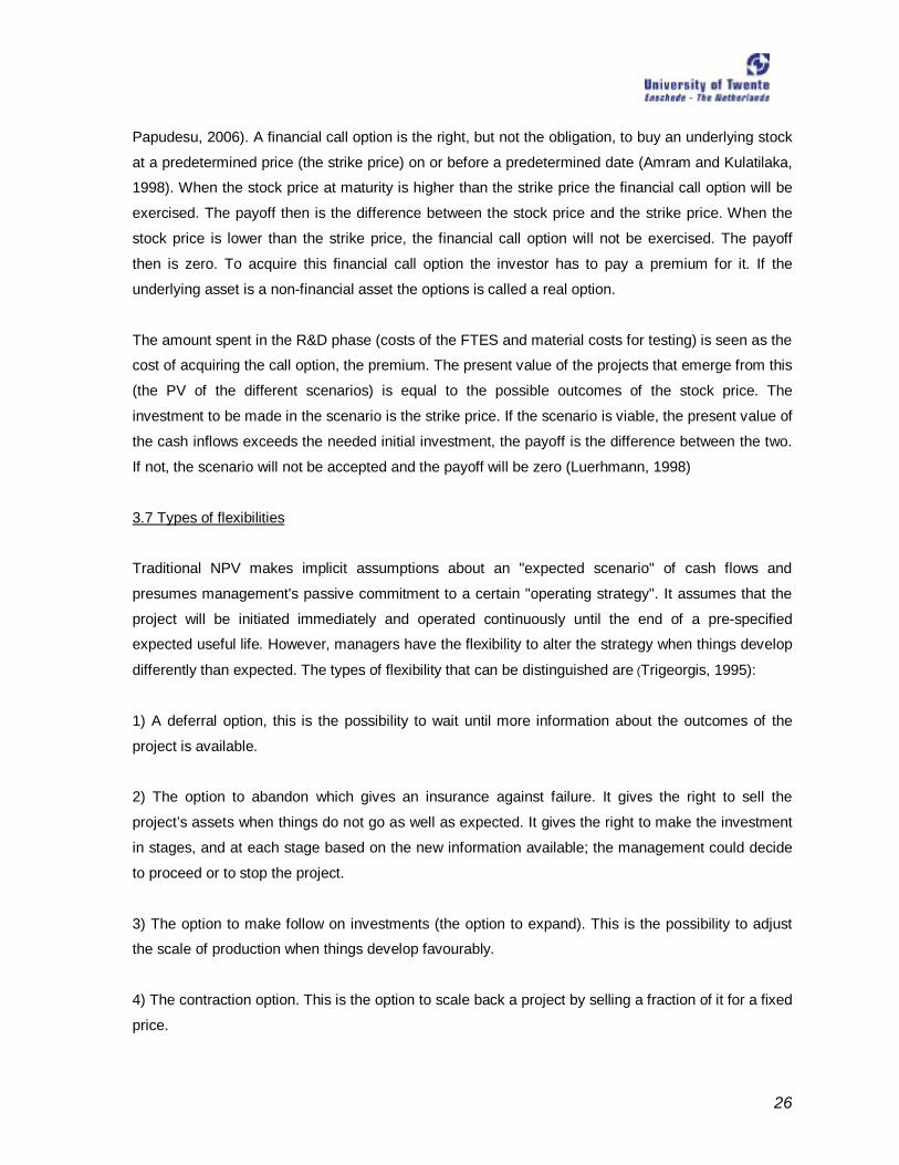
3.7 Types of flexibilities

Traditional NPV makes implicit assumptions about an "expected scenario" of cash flows and

presumes management's passive commitment to a certain "operating strategy". It assumes that the

project will be initiated immediately and operated continuously until the end of a pre-specified

expected useful life. However, managers have the flexibility to alter the strategy when things develop

differently than expected. The types of flexibility that can be distinguished are (Trigeorgis, 1995):

1) A deferral option, this is the possibility to wait until more information about the outcomes of the

project is available.

2) The option to abandon which gives an insurance against failure. It gives the right to sell the

project’s assets when things do not go as well as expected. It gives the right to make the investment

in stages, and at each stage based on the new information available; the management could decide

to proceed or to stop the project.

3) The option to make follow on investments (the option to expand). This is the possibility to adjust

the scale of production when things develop favourably.

4) The contraction option. This is the option to scale back a project by selling a fraction of it for a fixed

price.

27

5) Switching option. This is the option to vary the firm’s output or its production methods.

3.8 The Discount rate used in NPVx

The cash flows in the different scenarios have to be discounted by an appropriate discount rate, also

called the opportunity cost of capital. This discount rate is the same discount rate as being used in

computing the value of the underlying asset at the start of the binomial tree. There are two reasons

for discounting a cash flow (Brealy and Myers, 2002). The first one is because a dollar today is worth

more than a dollar tomorrow. A dollar today can be put in deposit and earn interest. The second

reason is that a safe dollar is worth more than a risky one.

3.8.1 Weighted Average Cost of Capital

A discount rate which is often used to discount projects is the WACC, the weighed average cost of

capital (Brealy and Myers, 2002). It is the calculation of a firm's cost of capital in which each category

of capital is proportionately weighted. The assets of a company are financed by debt and equity. The

WACC is the average of the costs of these sources of financing. The WACC shows the amount the

company has to pay for every dollar it finances. The WACC is calculated by multiplying the cost of

each capital component by its proportional weight and then summing:

WACC = Cost of equity * (equity/ (debt+equity)) + Cost of debt * (debt/ (debt+equity)) * (1-tax rate)

The WACC is often used by the management to determine the economic feasibility of new

opportunities. It can be used as the benchmark discount rate and new projects then are compared

with this WACC (Brealy and Myers, 2002 & Kodukala and Papudesu, 2006). If the risk of the new

project is relatively low and the project represents “business as usual”, the WACC is a proper

discount rate. For the projects with a higher risk, the WACC should be adjusted. So the WACC is the

appropriate discount rate to use for projects with risk that are similar to that of the overall firm.

3.8.2 Two types of risk

There are two different types of risks that can be distinguished, namely market risk and private risk

(Fabozzi and Mondigliani, 2002). Market risk is risk that cannot be diversified away. It is also called

systematic risk. It is the risk inherent to the entire market. The value of an investment may decline

because of economic changes that have impact on the whole market. Economic changes are for

example a decline in the interest rates or inflation. These events have influence on the entire

economy. Private risk or unique risk is the risk that is specific to a company. For example, the risk of

failing to develop a new technology is a private risk for a high-tech company. The risk of not finding a

28

large amount of oil in a particular oil field is the private risk for an oil company.

Investors are willing to pay a risk premium for cash flows which are market driven, but not for private

risk. This is because private risk could be diversified away by the investors. When there is no risk at

all, the risk free rate should be used to discount the cash flows because of the time value of money.

When the cash flows are market driven, a risk premium should be added to the risk free rate. The

size of the risk premium depends on the risk level of the project. When investors are taking higher

risks, they expect a higher return for taking the higher risks. So it is only reasonable to discount the

market driven project cash flows at a rate that is defined by the risk level of the projects (Kodukala

and Papudesu, 2006).

In a decision tree the cash flows must be discounted as you fold them back toward time zero. At

different points in the tree, different discount rates should be used (Margolis, 2003). The discount rate

depends on the type of risks in the decision tree. When the type of risk is unique/private risk, this risk

can be diversified away by the investors. The risk free rate should then be used as the discount rate.

When the cash flow stream in the tree is dictated by market risk, the non diversifiable risk, the WACC

should be used to discount the cash flows.

3.9 Conclusion

Traditional valuation methods like the Net Present Value (NPV) overlooked the flexibility of the

management to alter the course of a project in response to changing conditions. Projects are

assumed to proceed as planned, regardless of future events. The NPV method precludes operational

flexibilities such as the abandonment and the expansion of a project. These flexibilities of the

management have a value which is not captured in the traditional methods. With Real Options it is

possible to capture the value of these flexibilities. Real options see the investment in R&D projects as

making a relatively (compared with the total investment in the project) small initial investment which

creates opportunities to make a further investment in the next stage of the project. Till the moment

the product is being brought into the market, the organisation can decide to eventually cut the funding

in the project and not to market the project. This means, when the outcome of the R&D project is

negative, the NPV of this scenario will not be counted in the valuation of the project. The only losses

incurred then are the small initial investment.

It is important that the tool of Philips ADL includes the flexibility of the management to response to

changing conditions of the whole project. During the predevelopment stage more information can be

gathered about the progress of the project and based on this information, the management decides

whether the project is still worth funding. When it is known that the NPV of a scenario is negative, the

29

management could decide not making the initial investment in that particular scenario. This means

that the scenarios with a negative NPV should be left out in the calculation of the value of the project.

This can be achieved by modeling the option to abandon the project in the tool.

Another important issue is the discount rate used for the discounting of the cash flows of the project.

Projects have to be discounted at the right discount rate because any project investment requires

capital which is financed by investors. When investors are taking higher risks, they expect a higher

return for taking these higher risks. The discount rate depends on the type of risk that drives the cash

flows. There are two phases to be distinguished in the organisation. The first phase is the

predevelopment stage. The second phase takes place when the predevelopment is finished and the

product is bringing to the market. In the predevelopment stage I suggest to use the risk free rate and

in the second stage the WACC (which is currently used by Philips ADL) is an appropriate discount

rate, because in this second phase the cash flows are market driven.

In this part the theory of Real Options and the Discount Rate has been discussed. In the next chapter

the tool will be discussed in more detail using the theory.

30

Chapter 4 Application of the theory

In this chapter the research questions “Is the current model, which is based on Real Options theory,

correct?” and “Which improvements are needed for the current tool?” will be answered. In this

chapter, the parameters in the formula mentioned in the last chapter will be explained more explicitly

one by one. In paragraph 4.1 the mathematics behind the calculation of the chances for the different

scenarios are described. Paragraph 4.2 will explain how the Net Present Value of the different

scenarios is calculated. In paragraph 4.3 the current Discount Rate used to discount the cash flows in

the different scenarios is discussed. Paragraph 4.4 gives a summary of the current tool. Finally, this

chapter ends with a conclusion in paragraph 4.5.

4.1 The calculation of the chances of the different scenarios (px)

When each key uncertainty of the project has influence on just one scenario, the success chance of a

scenario is simply calculated by multiplying “the success chances of all the key uncertainties which

are necessary for that particular scenario” and then multiplying this chance with the failure chances of

the previous scenarios. However, in most situations, the key uncertainties have influence on multiple

scenarios. This is the reason that the formula mentioned in paragraph 3.2 is not entirely correct. In

this paragraph the adjustment of the formula will be discussed.

px is defined as the feasibility of scenario x and px’ as the success chance of scenario x GIVEN

scenarios 1, 2…x-1 failed.

The feasibility of scenario x is defined as the chance that the key uncertainties for scenario x are all

successfully resolved. The success chance of scenario x is defined as the chance that scenario x is

executed. At this moment the chance of success for scenario 2 is calculated by “the chance that

scenario 1 is not feasible” * “the feasibility of scenario 2”, (1- p1) * p2. Adjusting this formula with

conditional chances gives the following formulas:

p1’ = p1

p2’ = p (S2 feasible | S1 not a success)

= p (S2 feasible & S1 not a success) / p (S1 not a success)

= p (S2 feasible & S1 not a success / (1-p1’)

p3’ = p (S3 feasible | [S1 not a success & S2 not a success])

= p (S3 feasible & S1 not a success & S2 not a success) / p (S1 not a success & S2 not a success)

31

Because p (S1 not a success & S2 not a success) = p (S1 not a success) * p (S2 not a success | S1 not

a success) = (1-p1’) * (1-p2’), this gives the following formula for p3’:

p3’ = p (S3 feasible & S1 not a success & S2 not a success) / [(1-p1’) * (1-p2’)]

pN’ = p (SN feasible | [S1 not a success & S2 not a success &… & SN-1 not a success])

= p (SN feasible & S1 not a success & S2 not a success &… & SN-1 not a success) / p (S1 not a

success & S2 not a success &… & SN-1 not a success)

The old formula is: Value project = p1 * NPV1 + p2 * (1- p1) * NPV2 + p3 * (1-p2) * (1- p1) * NPV3 + …+

px * (1-px-1) * (1-px-2) * …* (1-p1) * NPVx

This formula is only allowed when all the key uncertainties for each scenario are different from the

key uncertainties of the other scenarios. However, in almost all the projects, there is always at least

one uncertainty which has influence on multiple scenarios. The conditional chances of the different

scenarios are now calculated by making use of VBA Excel. See appendix B for the code. After the

adjustment has been made, this gives the following decision tree (figure 13).

Predevelopment Outcome

Go

No Go

Go

Go

Go

Quit

Quit

Quit

p1’

p2’ * (1-p1’)

p3’ * (1-p2’) * (1-p1’)

NPV1

NPV2

NPV3

Figure 13, Adjusted Decision tree Philips ADL

32

New formula project is:

Value project = p1’ * NPV1 + p2’ * (1- p1’) * NPV2 + p3’ * (1-p2’) * (1- p1’) * NPV3 + …+ px‘ * (1-px-1’) * (1-

px-2’) *…* (1-p1’) * NPVx

px’ = The success chance of scenario x GIVEN scenarios 1…x-1 failed.

NPVx = Net present value of scenario x

This formula is still not totally correct, because the cash flows of the different scenarios are not

discounted in the predevelopment stage. In paragraph 4.5 a suggestion is given of how to adjust the

formula.

In example 5 the calculations of the chances for the different scenarios are explained more explicitly. Example 5

Figure 14, summary example of a fictive project

A project has 4 key uncertainties, uncertainty A, B, C and D. The NPV of scenario 1 is 48 million, the

NPV of scenario 2 is 40 million and scenario 3 has a NPV of 12 million. Scenario 1 requires

uncertainty A, B and C, scenario 2 requires A and D and scenario 3 B and C. See figure 14. The “1”

means that the key deliverable is required for the scenario.

If the success chance of a scenario is calculated by multiplying the chance of success from one

scenario with the failure chance of scenario, the chances calculated will be too optimistic.

• Success chance of scenario 1 = success chance of key uncertainty A* success chance of

key uncertainty B* success chance of key uncertainty C. This gives 0,7* 0,6* 0,8 = 33,6%

Scenario 1Scenario 2 Scenario 3NPV 48 40 12

Key deliverable Estimated Probability of Success (Current Date)

A 70% 1 1B 60% 1 1C 80% 1 1D 70% 1

33

• Success chance of scenario 2 is: (1 - success chance of scenario 1) * success chance of key

uncertainty A *success chance of key uncertainty D = (1- 0,336)* 0,7* 0,7 = 32,5%

• Success chance of scenario 3: (1 - success chance of scenario 1)*(1 - success chance of

scenario 2)* success chance of key uncertainty B* success chance of key uncertainty C =

16,3%

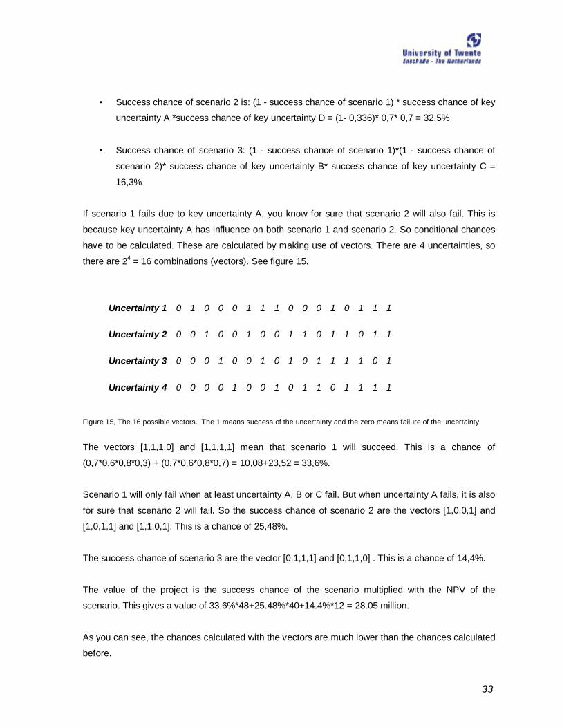
If scenario 1 fails due to key uncertainty A, you know for sure that scenario 2 will also fail. This is

because key uncertainty A has influence on both scenario 1 and scenario 2. So conditional chances

have to be calculated. These are calculated by making use of vectors. There are 4 uncertainties, so

there are 24 = 16 combinations (vectors). See figure 15.

Uncertainty 1 0 1 0 0 0 1 1 1 0 0 0 1 0 1 1 1

Uncertainty 2 0 0 1 0 0 1 0 0 1 1 0 1 1 0 1 1

Uncertainty 3 0 0 0 1 0 0 1 0 1 0 1 1 1 1 0 1

Uncertainty 4 0 0 0 0 1 0 0 1 0 1 1 0 1 1 1 1

Figure 15, The 16 possible vectors. The 1 means success of the uncertainty and the zero means failure of the uncertainty.

The vectors [1,1,1,0] and [1,1,1,1] mean that scenario 1 will succeed. This is a chance of

(0,7*0,6*0,8*0,3) + (0,7*0,6*0,8*0,7) = 10,08+23,52 = 33,6%.

Scenario 1 will only fail when at least uncertainty A, B or C fail. But when uncertainty A fails, it is also

for sure that scenario 2 will fail. So the success chance of scenario 2 are the vectors [1,0,0,1] and

[1,0,1,1] and [1,1,0,1]. This is a chance of 25,48%.

The success chance of scenario 3 are the vector [0,1,1,1] and [0,1,1,0] . This is a chance of 14,4%.

The value of the project is the success chance of the scenario multiplied with the NPV of the

scenario. This gives a value of 33.6%*48+25.48%*40+14.4%*12 = 28.05 million.

As you can see, the chances calculated with the vectors are much lower than the chances calculated

before.

34

The value calculated is always the optimal value. There are no other combinations of the scenarios

that will give a higher option value. The optimal combination always gives the priority to the scenario

with the highest NPV and so on. The explanation for this is that a change in the sequence of the

scenarios (for example do scenario 3 first and then 2 and then 1) will not change the success vectors.

These vectors will still be the same. As a result this will not lead to a higher option value.

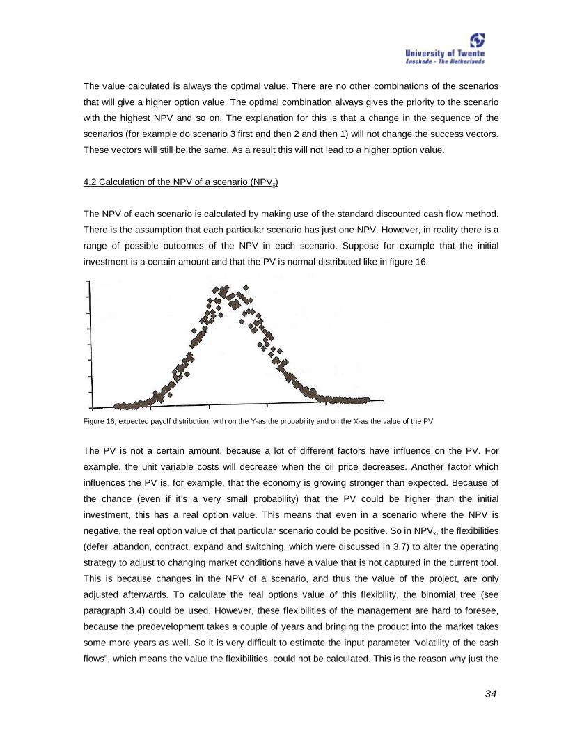
4.2 Calculation of the NPV of a scenario (NPVx)

The NPV of each scenario is calculated by making use of the standard discounted cash flow method.

There is the assumption that each particular scenario has just one NPV. However, in reality there is a

range of possible outcomes of the NPV in each scenario. Suppose for example that the initial

investment is a certain amount and that the PV is normal distributed like in figure 16.

Figure 16, expected payoff distribution, with on the Y-as the probability and on the X-as the value of the PV.

The PV is not a certain amount, because a lot of different factors have influence on the PV. For

example, the unit variable costs will decrease when the oil price decreases. Another factor which

influences the PV is, for example, that the economy is growing stronger than expected. Because of

the chance (even if it’s a very small probability) that the PV could be higher than the initial

investment, this has a real option value. This means that even in a scenario where the NPV is

negative, the real option value of that particular scenario could be positive. So in NPVx, the flexibilities

(defer, abandon, contract, expand and switching, which were discussed in 3.7) to alter the operating

strategy to adjust to changing market conditions have a value that is not captured in the current tool.

This is because changes in the NPV of a scenario, and thus the value of the project, are only

adjusted afterwards. To calculate the real options value of this flexibility, the binomial tree (see

paragraph 3.4) could be used. However, these flexibilities of the management are hard to foresee,

because the predevelopment takes a couple of years and bringing the product into the market takes

some more years as well. So it is very difficult to estimate the input parameter “volatility of the cash

flows”, which means the value the flexibilities, could not be calculated. This is the reason why just the

35

NPV method is used to calculate the NPV of a particular scenario.

4.3 Current risk adjusted discount rate

There are two phases to be distinguished. The first phase is the predevelopment stage. The second

phase takes place when the predevelopment has been finished and the product is being brought into

the market. The cash flows of the different scenarios are discounted to this moment, the moment the

product is being brought into the market. In this phase the WACC is used as the discount factor for all

the different projects. This WACC is dictated by Philips. In this phase the cash flows are market

driven (for example the market demand). However, some projects are much more risky than the

average projects. So for the more risky projects a discount rate higher than the WACC should be

used. For the safer projects, the WACC is a proper discount rate.

In the predevelopment the project success is determined by the effectiveness of the new technology

and the efficiency of the organisation in completing the project. As a result, the predevelopment

phase is considered to be controlled by private risk and not to market risk. The cash flows of the

project are not subject to the market forces in this phase. When this is the case, the risk free rate

should be used (discounting because of the time value of money) to discount cash flows in this stage.

In the current model the cash flows of the different scenarios are not discounted in this first stage of

the project. This is caused by the fact that the duration of this first stage for the different projects is

not known. However, the cash flows should be discounted at a risk free rate because otherwise the

NPV calculated will be too optimistic.

4.4 Value of the total project

The flexibility to respond to changes in the technology outlook are captured in the current tool, see

the decision tree in figure 8. It captures the value of the option to abandon the project. The tool

quantifies the technological risks and creates value by structuring the predevelopment stage into

go/no-go decisions points that exploit the option to abandon the project (Boer, 2003). This value is

directly captured in the valuation of the project because the negative scenarios are left out in the

expected value of the project. This approach of computing the expected value of the project is a form

of real options thinking.

An option is the opportunity to make a decision after you see how events unfold. On the decision

date, if events turned out well, you will make one decision, but if they turned out poorly you will make

another. Valuating this option (the option to abandon if the situation develops unfavourably) is not

36

equal to the value that is given to a project in the current situation. In the current situation the way

“real options thinking” would value the project as a whole is calculated. This is different from the value

of the option to abandon the project. To calculate this option value, the value of the opportunity

without this option should be calculated first. The difference between these amounts then is the value

of the option to abandon.

Example 6

A project has 5 different scenarios, see figure 17. A standard NPV analysis which taken into account

all the possible scenarios will value this as 48 * 0,336+ 40 * 0.2548 *1 2 * 10.08 +-50 * 0.984 + -10 *

0.11 = 16.51 million.

Scenario NPV Success chance (%)

Scenario 1 48 33,6

Scenario 2 40 25,48

Scenario 3 12 10,08

Scenario 4 -50 19,84

Scenario 5 -10 11

Figure 17, summary example 6.

In real options thinking the flexibility to change the course of action is taken into account. So the

negative outcomes will be avoided, because if the outcome is bad, the management will stop making

further investment in the project (abandon). Real options would value this project as 48 * 0,336 + 40 *

0.2548* 12 * 10.08 = 27.53 million. So the option to abandon is worth 27.53 – 16.51 = 11.02 million.

4.5 Conclusion

The current tool is correct, however there are some improvements which can be made. First of all the

chances assigned to the different scenarios are not entirely correct, because in most situations the

key uncertainties of the project have influence on multiple scenarios. This means that conditional

chances have to be calculated instead of it. During this thesis, this problem has been solved. The

chances are now computed by making use of VBA Excel (see also Appendix B). This code is written

by Ruud Gal (the innovation manager).

The second improvement that can be made is the discounting of the cash flows in the first stage of

the projects, the predevelopment stage. In the current model the cash flows of the scenarios are not

37

discounted in this stage, because the duration of this stage is not known for certain. However, as

mentioned before, the cash flows should be discounted using the risk free rate, because of the time

value of money. This has not yet been implemented. A possible way to adjust the formula is as

follows:

Adjusted Value project = [p1’ * NPV1 + p2’ * (1- p1’) * NPV2 + p3’ * (1-p2’) * (1- p1’) * NPV3 + …+ px’ * (1-

px-1’) * (1-px-2’) *…* (1-p1’) * NPVx] / (1+riskfree rate)d

where d = expected staying time of the project in the predevelopment stage.

In the current situation, the NPV of each scenario is the NPV at the moment the product is bringing to

the market. By discounting the expected value of the total project at a risk free rate during the

predevelopment stage, the NPV of the project at the start of the predevelopment is computed.

38

Chapter 5 Subjective probability assessment

5.1 Introduction

In this chapter the two questions “Which methods could be used to improve the input parameter

estimated chance of technical success?” and “Is the method applicable for Philips ADL?” will be

answered. This chapter consists of two parts. The first part is the theoretical part. In this part the

methods which can be used to estimate the technical success chance will be discussed. In the

second part the results of the pilot study is shown.

Part I: Theoretical part

5.2 Introduction subjective probability

The elicitation and use of expert opinions is increasingly important. Often new projects are so unique,

which makes it almost impossible to use historical data of projects to judge about the success chance

of the new projects. The technologists are turning in greater numbers to “expert systems” (Cooke,

1991). These experts have a lot of accumulated knowledge, which can be very useful in judging the

new projects.

5.3 Definition subjective probability

The definition of Laplace of probability is the ratio of the number of cases favorable to the event to the

number of all possible cases; each case is assumed to be equally likely. This is also called the

objective probability. When throwing a dice, the chance on a six is 1/6. There is no discussion about

it. On the other hand there is the subjective probability. This probability expresses the feeling of an

individual. The definition of subjective probability is (Hampton, Moore and Thomas, 1973):

Subjective probability is considered a quantification of uncertainty. It represents the extent to which a

coherent person believes a statement is true, based on the information available to him at that time.

A subjective probability describes an individual's personal judgement about how likely a particular

event is to occur. It is not based on any precise computation but is often a reasonable assessment by

a knowledgeable person. The probability is normally expressed on a scale between the 0 and 1. An

infrequent event will have a subjective probability close to zero and an event that is very common will

have a subjective probability close to one. This type of estimating is called point estimation. It is also

39

possible that the estimator has to assess the whole distribution of a particular event (by using

methods like psychometric ranking and probability density functions). But the rest of this chapter will

be focused on point estimation, because in the current situation of ADL the project leader estimates

the chance of success of a key uncertainty as just one number.

5.4 Methods for eliciting subjective chances

There are different methods that can be used to estimate subjective chances. It is possible to

estimate the chances individually or in a group (Hampton, Moore and Thomas, 1973).

5.4.1 Individual methods

When using the individual method, there is a distinction between the direct and indirect method. In

the direct method the person is directly interrogated concerning his judgments. The decision maker is

asked to express his beliefs by a number between 0 and 1. In the indirect method the person’s

assessment is concluded from his preferences between possible decisions. This technique is divided

into two methods, the lottery technique (bet method) and the equivalent urn method.

The Bet method

In this technique the decision maker answers a series of yes-no questions in terms of simple betting

odds. His subjective probability for the occurrence of the event is then implied from the odds required

to make him indifferent between two offered bets. For example: If sales next month exceed 1000

units, he gets 50 dollar, otherwise nothing. So there exists an amount in dollar (Y), which makes the

two bets equally attractive to him.

EV (expected value) =p50 + (1-p) 0, where

p= probability that sales next month exceed 1000 and Y= amount of dollar receiving. EV=Y, p= Y/50.

Equivalent urn method

In the equivalent urn, the urn consists of the chances of occurrence of the events. The urn contains

several colored balls, within each ball means the occurrence of an event. The judger assesses what

mix of balls will make the urn equivalent to his feelings.

The advantage of these indirect methods is that the measurement error, the discrepancy between

reported and actually held judgment, will be obviated by these techniques (Savage, 1954).

40

5.4.2 Group methods

When using the group method approach, there are three different methods distinguished (Van de Ven

and Delbecq, 1974).

Interacting groups

At the beginning of the discussion, the statement of the problem is made. This is followed by an

unstructured group discussion for generating information and pooling judgments among participants.

The meeting ends with a majority voting procedure. This method is an unstructured face-to-face

group meeting. The administrative costs and time for the preparation are low and the time to obtain

the results is immediately after the meeting finishes (which takes approximately 1,5 hours).

Nominal Group Technique (NGT)

This method is a structured face-to-face group meeting. This is a meeting with a structured format. At

the beginning of the discussion, the statement of the problem is made. Then the members of the

group generate their ideas of a problem individually on a paper (in case the problem is to estimate

chances, the members starts with making the estimates individually on a paper). After this phase, the

members present their ideas (estimates) to the group. When they have presented their ideas

(estimates), there is a discussion of the ideas (estimates). The session ends with a voting procedure.

The administrative costs and time for the preparation are medium and the time to obtain the results is

right after the meeting finishes (which takes approximately 1,5 hours).

Delphi method

The core of this method is a repeated consolation of experts (Dalkey, 1968). Each participant starts

with filling out a questionnaire and gets feedback concerning the answers (estimates) of all the

participants. With this new information the participant fills out the questionnaire again, but now with

explanation on the questions which were completely different from the other participants. This

information serves as useful information for the other participants. The participant can change his

beliefs after the evaluation of the new information from the others. This process is continuously

repeated as long as necessary. Unlike the Interacting Group and the NGT, the participants in the

Delphi method do not meet face-to-face for group decision-making. The administrative costs and time

for the preparation are high and the time to obtain the results is a few months.

In the three group methods discussed before, it is possible to assign higher weights to a judger if the

judger is a specialist on one of the technological area (Winkler 1968). This can be done by the

participants of the group individually, or by someone outside the group.

41

5.5 Effectiveness of the methods in terms of accuracy

Gustafson et al (1973) tested the effectiveness of independent individuals, interacting, NGT and the

Delphi method on a problem of subjective probability estimation. The criteria he used were the

absolute mean percentage error between methods and the variance of estimates across groups. The

mean percentage error indicates the degree of bias and the variance measure indicates the degree

of consistency (the smaller the differences in the estimates between the members of the group, the

more consistent the estimates are). The results showed that the NGT was the best in terms of the

lowest percentage of errors and variability of estimates. Second best was the interacting group and

third was the independent individual. The Delphi method was the worst. This was caused by the fact

that a derivative process called Estimate-Feedback-Estimate was used instead of the real Delhi

method, because the Delphi method was too expensive. In the experiments carried out by Dalkey

(1968) the respondents estimated the accuracy of a set of facts. The results showed that the

estimates with more persons are more accurate than the estimation carried out by one person.

5.6 Effectiveness of the methods in terms of ideas / information generated

The ideas / information generated in a process are a very important gauge. The greater the quantity

of ideas / information generated, the greater the number of ideas / information are considered in

making a decision. This implicates a better decision (Van de Ven and Delbecq, 1971). Osborn (1957)

showed that an average person could think up twice as many ideas when working in a group instead

of working alone. These are also the results of Taylor, Berry and Block (1958). Their statement was

that group participation does facilitate the production of ideas. Taylor, Berry and Block (1958) also

compared the nominal group method with the interaction group. They compared these two methods

in terms of three measures, namely the mean number of unique ideas, the mean total number of

ideas and the quality of ideas. Based on these three measures, the nominal group was significantly

superior to the interaction group in generating information relevant to the problem. A study from Van

de Ven and Delbecq (1974) also showed that the NGT and the Delphi method were the methods that

generated the most ideas. Their study also measured the perceived group satisfaction. This is the

satisfaction the participants perceive with the group process and the decision outcomes. This is

important because a higher satisfaction will lead to a higher probability of solution adoption.

5.7 Phases in estimating subjective probabilities

The process of estimating probabilities of technical success for R&D projects can be being composed

in four phases, the perception phase, the evaluation phase, the transformation phase and the review

42

phase (Rubenstein and Schroder, 1977):

1. In the perception phase the perceiving of the project attributes takes place.

2. In the evaluation phase qualitative judgment about the technical chance of success will be

made.

3. In the transformation phase the qualitative judgment will be transformed into numerical

values. These values mean the degree of belief, also called the subjective probabilities.

4. In the review phase, the actual subjective probabilities are scrutinized with respect to their

communicability. The communicated subjective probability may differ from the actual

subjective probability if they think this is necessary.

5.8 Variables, which influenced the subjective probability

There are three different sorts of variables, which have influence on the communicated subjective

probability of technical success of the project (Rubenstein and Schroder, 1977). These are the

personal variables, organization variables and situational variables. Personal variables have a direct

influence on the communicated subjective probability, while organizational and situational variables

act indirectly via the personal variables.

• Personal variables: These are the characteristics of the assessors which have influence on

the assessor’s ability to perceive and evaluate a project’s attributes and to transform their

belief into a numerical value, as well as their willingness to transmit their actual subjective

probabilities of technical success. Most important among them are education and previous

experience. Psychological aspects of the probability assessment are also an important

aspect. The finding of Kahneman and Tversky (1972) showed that people tend to solve

complex tasks of assessing probabilities by simplifying the assessment problem with the

application of a few heuristic principles. For example the heuristic representatives, the

probability is determined by the degree to which is similar in essential characteristics to its

parent population. This can lead to a cognitive bias.

• Organizational variables are the variables such as the assessor position in the company

hierarchy.

43

• Situational variables express the influences of factors, which are specific to the project to be

assessed. For example the assessor specific relation toward the project like the project

responsibility or his position with respect to the project generation.

Assessors who generated the project idea or did participate in the idea generation will assign a

higher chance of technical success than a nonoriginator. This is because they have the tendency to

upgrade positive and downgrade negative circumstances. When it is necessary they will

communicate a higher probability of success than the actual subjective probability to get acceptance

for the project. A test conducted by Rubenstein and Schroder (1972) showed that in 53 out of the 90

comparisons between an originator and a nonoriginator the estimate given by the originator was

higher. In 20 comparisons there were no differences and in just 17 cases the nonoriginator was more

optimistic.

Assessors with project responsibility (responsibility to project implementation with the planning and

control functions included) will assign higher probabilities of success. This is because of their

enthusiasm. Enthusiasm is associated with downgrading negative and upgrading positive aspects.

This optimism is of more weight than the insurance against potential failure of the project by

assessing lower probability of success (results shown by Rubenstein and Schroder).

In the next part the application of the theory takes place. Part II: Application of the subjective probability theory

Using the theory from Rubenstein and Schroder (1972) I will discuss the assessment of the chance of

success of the different key uncertainties by the project leaders in more detail.

The project leader is the one who determines the most important key uncertainties of the project.

After this process, he will assign the chance of technical success to each key uncertainty. At this

moment the project leaders are using the direct individual method. The assessor is directly

interrogated concerning his judgments. The decision maker is asked to estimate the current chance

of technical success by a number between 0 and 1. They also have to give a prediction of the chance

of success three months from now, assuming that everything is going perfect.

The project leaders are well educated and very experienced. They do have the expert knowledge, so

they have the ability to estimate the chance of success of the different key uncertainties. However,

some projects have a very broad scope. It is possible that due to their lack of knowledge, they are not

44

capable of judging the key uncertainties properly. So in this case it is the lack of ability to give a

proper estimation.

As Rubenstein and Schroder point out, the communicated subjective probability is not always equal

to their actual degree of belief. Because of information asymmetry (the project leader has more

information about the project than the innovation manager has), it is possible for the project leader to

manipulate the estimated chances. When it is necessary to get acceptance for the project, the project

leader will assign relatively high probabilities to the key uncertainties because these higher chances

will lead to a higher financial option value of the project. A higher value indicates a better project, so

the project is getting more FTES allocated. When the project got the FTES allocated, the project

leader will be more cautious in the estimates to insure him against potential failure. In the current

situation the project leader is the only person who estimates the chances. So there is no control over

these assessed probabilities.

The project leader is always involved in the originating of the project and he has a high project

responsibility. As a result of this, the project leader will have the tendency to upgrade positive and

downgrade negative circumstances. I think this should not always be seen as a disadvantage.

Sometimes it is necessary to be positive, because this will stimulate the motivation of the whole

project team.

In the past (before the current model was introduced) the project leaders did not have to estimate the

chance of technical success explicitly. As a result, they are not really familiar with the process of

estimating chances. The more they estimate, the more feeling they will develop for this process. This

will result in better estimates.

In the current situation the project leader is the only person who estimates the chances of success. In

this situation it can easily lead to the manipulation of the chances. This is the reason why I suggested

to introduce a small committee. A committee helps the project leader to estimate chances and the

defining of the key uncertainties of the project. In the next paragraph I will show the results of the pilot

study.

5.9 Pilot study

I introduced a small committee because the estimation of chances with just one person can lead to

manipulation or incorrect estimates. This is also what the literature suggests, using the group

approach in favour of the individual judgment. Studies from Gustafson et al (1973) and Dalkey (1969)

showed that estimates made by individuals are less accurate than the group method. And besides,

45

by using the group approach more information relevant for the problem will be generated (Delbecq

and Van de Ven, 1971). The greater the quantity of information generated, the greater the number of

information are considered in making a decision. The other members of the committee can help the

project leader to define the most important key uncertainties.

The group method I chose was the nominal group technique. The reason for this method is that the

Delphi method takes too long to get results and the costs involved are very high. The other technique

left was the interaction group. The study from Gustafson (1973) showed that the nominal group

technique has the lowest percentage of measurement errors. Delbecq and Van de Ven (1974)

showed that the nominal group technique has the highest perceived satisfaction by the participants.

To improve the validity of the estimates, a small committee was established. Besides the project

leader, two extra estimators were added to the estimation process. These two estimators have a lot

of technological expertise and experience, and also very important: they are independent.

At the beginning of the group meeting the project leader started with his introduction of the project.

He defined his key uncertainties of the project. After this, the rest of the group gave their view on the

project. After the evaluation of these uncertainties, they started with the assessment of the chances

of each key deliverable individually. One of the members of the group did not really want to estimate

certain uncertainties because he does not possess the expert knowledge for it. For the key

deliverables, where the estimates significantly differed from each other (10% or more), a general

discussion was required to explain the differences. There were hardly any significant differences

because the other independent estimator was not really independent. He was already involved in the

project. After the discussion, with the new information generated in the discussion, each individual

estimated the success chances again. The end result was the pooled outcome of the individual

estimates. The assessor who did not really want to estimate, mentioned that he only wanted to

estimate, if there would be lower weights assigned to his opinions. After the meeting, I asked about

the satisfaction perceived with this group process. They thought it was useful.

5.10 Conclusion

There are different methods that could be used to improve the estimation of the project leaders. It is

possible to estimate individually and in a group. Literature study showed that the group approach is

more accurate than the individual method. The three methods for the group approach are the

Interaction group, the Delphi method and the Nominal group technique. Literature study showed that

the Nominal group technique (NGT), a structured face-to-face group meeting, is the best method of

these three methods.

46

The pilot study showed that the meeting helped to evaluate the key deliverables. Some uncertainties

were not really uncertainties and some uncertainties were “forgotten”. Using the method to estimate

the chances is a more difficult matter, because the independent estimators only want to assess the

uncertainties when they have the expert knowledge. To implement the Nominal Group technique I will

advise the following method:

Search for two independent estimators who are independent of the project and have a lot of

knowledge. Before the meeting the two independent estimators have to be informed by the project

leader about the project (by sending some important documents), so they can be well prepared for

the meeting. The actual meeting then starts with a short introduction of the project by the project

leader. After this introduction, the members discuss about the key uncertainties of the project. When

they have reached consensus about the key uncertainties, they individually estimate the success

chance of each key uncertainty. The success chance of each key uncertainty then is the mean of the

estimates of the members of the group.

47

Chapter 6 Conclusions and Recommendations

Conclusions

In chapter 3 the research question “Which are the most important characteristics of Real Options for

the valuation of R&D products?” is discussed. Chapter 4 answered the research questions “Is the

current model, which is based on Real Options theory, correct?” and “Which improvements are

needed for the current tool?”. In chapter 5 the research questions “Which methods could be used to

improve the input parameter estimated chance of technical success?” and “Is the method applicable

for ADL?” are discussed.

Question1: Which are the most important characteristics of Real Options for the valuation of R&D

products?

Answer: The most important characteristics of Real Options are the uncertainty of the underlying

asset (for example the outcome of the R&D project) and the flexibility of the management to deal with

this uncertainty. Real Options capture the value of the flexibility of the management to alter the

course of a project in response to changing conditions. After a small initial investment (compared with

the total investment in the project), the management can gather more information about the progress

of the project and market characteristics and based on this information change the course of action.

Question 2 and 3: Is the current model, which is based on Real Options theory, correct? and Which

improvements are needed for the current tool?

Answer: The current tool is correct; however some improvements could be made. The first

adjustment which could be made is the assigning of the chances to the different scenarios. Before I

started with this thesis the chances assigned to the different scenarios were not entirely calculated

correctly, because in most of the projects the scenarios have key uncertainties which influenced

multiple scenarios. This means that conditional chances have to be calculated. These conditional

chances are now calculated by making use of VBA Excel. The second improvement that can be

made is the discounting of the cash flows in the first stage of the projects. In the current model the

cash flows of the scenarios are not discounted in the first stage, because the duration of this first

stage is not known. However, the cash flows should be discounted using the risk free rate because of

the time value of money.

Question 4: Which methods could be used to improve the input parameter “estimated chance of

technical success”?

Answer: Literature study showed it is possible to estimate individually or in a group. The literature

48

study showed that the group approach is more accurate than the individual method. The three

methods for the group approach are the Interaction group, the Delphi method and the Nominal group

technique. The Nominal group technique (NGT), a structured face-to-face group meeting, is the best

method of these three methods.

Question 5: Is the method applicable for ADL?

Answer: A pilot study was conducted to see if the NGT method is applicable for Philips ADL. The pilot

study showed that the meeting was really useful in the evaluation of the key deliverables. Some

uncertainties were not really uncertainties and some uncertainties were “forgotten”. Using the method

to estimate the chances is a more difficult matter, because the independent estimators only want to

assess the uncertainties when they have the expert knowledge.

Recommendations

After all the research I have come up with three recommendations:

1. Before I started with this thesis the chances assigned to the different scenarios were not

calculated entirely correct, because in most of the projects the scenarios have key

uncertainties which influenced multiple scenarios. This means that conditional chances have

to be computed.

2. The second recommendation is the introducing of a discount rate in the predevelopment

stage. In the current model, the cash flows of the scenarios are not discounted in this stage,

because the duration of this first stage is not known for certain. However, I recommend using

a risk free rate to discount the cash flows in this phase, because of the time value of money.

A possible way of adjusting the formula is as follows:

Adjusted Value project = [p1’ * NPV1 + p2’ * (1- p1’) * NPV2 + p3’ * (1-p2’) * (1- p1’) * NPV3 +…+

px‘ * (1-px-1’) * (1-px-2’) *…* (1-p1’) * NPVx] / (1+riskfree rate)d

where d = expected staying time of the project in the predevelopment stage.

3. In the current model the project leader is the only person who estimates the success chances

of the key deliverables. Because of information asymmetry it is possible for the project

leaders to manipulate these chances. This is the reason why I suggest introducing a group

process for the big (in terms of NPV) projects. By estimating the chances in a group, these

manipulations will be reduced. And besides this advantage, the measurement errors will also

49

be reduced. Finally, the members of the group could help the project leader to define the

most important uncertainties of the project. The pilot study showed that this method is very

useful.

Interesting issues

There are also some other interesting issues I want to mention. The first one is the introducing of

FTES needed for each key uncertainty. At this moment the FTES needed for the whole project is

given, but I think it is better to split these FTES into the FTES per key uncertainty. In the case where

it is not possible to solve all key uncertainties, this information is necessary to determine a scheme

(to determine the sequence in which the different uncertainty should be solved), which optimizes the

option value of the project. The current tool is used as a management portfolio tool. By making these

changes, the tool can also be used as a project tool. The second subject is using a distribution of the

chances instead of the current point estimation. With a distrubution of the chances a sensitivity

analysis can be conducted (using Crystal Ball for example). The option value is calculated by the

chances given by the assessor, but these chances can vary. What is the impact on the option value

when the chance of one uncertainty is not 60% but 50%? What is the impact on the option value

when two uncertainties vary together? With sensitivity analysis the minimal, most likely and maximum

option value of the project, could be computed. With this information it is possible to compare projects

with each other more explicitly.

Further research

There are two subjects I would like to mention for further research:

1 Collect the data of the project leader’s estimates per key uncertainty. As mentioned before, I

recommend estimating the success chances of the different key uncertainties in a group.

This process of estimating will increase the accuracy of the estimates. However, this process

takes a lot of time from the independent estimators. This means it cannot be used for each

individual project. It may be possible, by collecting the data of the e project leader’s estimates

for a long period of time, and analyzing this collected data with the use of statistics, to tell

more about the reliability of the estimates of the project leaders.

2 Check for the possibility to introduce real options value in NPVx. It is very difficult to estimate

the volatility factor of a new project. An approach could be to use the data from historical

projects, which is assumed to have cash flows similar to the project being considered.

However, each project is very unique, so I am not sure if this information acquired is valid.

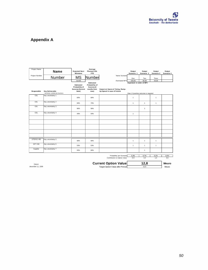
50

Appendix A

Project Name

Name Expected Next Milestone

Average Planned CDL

FTEOutput

Scenario 1Output

Scenario 2Output

Scenario 3Output

Scenario 4Project Number

Number MS NumberName Scenario

One Two Threenov-06 Estimated NPV 100,00 50,00 25,00

Responsible Key Deliverable

Estimated Probability of

Success (Current Date)

Estimated Probability of

Success (3 months from

now)Impact on Specs & Timing, Ramp-Up Speed in case of Failure

Important: in order of NPV

- technical, commercial, business Give 1 if positive outcome is requiredCDL Key uncertainty 1

60% 80% 1 1

CDL Key uncertainty 260% 70% 1 1 1

CDL Key uncertainty 380% 90% 1

CDL Key uncertainty 4 40% 50% 1

GTD/SG HID Key uncertainty 590% 90% 1 1 1

GPT HID Key uncertainty 653% 53% 1 1 1

Supplier Key uncertainty 750% 80% 1

Probability per Scenario 6,9% 8,7% 6,2% 0,0%Contribution to Option Value 6,9 4,4 1,5 0,0

Datum Current Option Value 12,8 Meurodecember 11, 2006 Target Option Value after Period 21,5 Meuro

51

Appendix B

The code is based on example 5, searching for non overlapping vectors and attribute these vectors to

the different scenarios.

This is a user-defined function, which calculates the probability a scenario will be selected / occur.

Function OptionProbability(ByVal RiskVector As Range, _

ByVal RisksPerOutputScenarioMatrix As Range) As Single

ColumnIndex Nr of scenarios (the one for which probability of success is

calculated)

RiskVectorLength Number of key deliverables that have a probability of success

PossibleOutputScenaioVectors A set of output scenarios (combinations of 1 and 0s) that are

possible and relevant for the output scenario for which probability

of success is to be calculated

ProbabilityNonOverlapWithEarlierScenario If a possible output scenario is overlapping (already

addressed) by an earlier/more preferred output scenario

it's impact on the probability of success to be calculated

will be ignored

Dim i, j, ColumnIndex, ArrowRoy, ArrowCol As Long, _

RiskVectorLength As Integer, _

PossibleOutputScenarioVectors() As Single, _

ProbabilityNonOverlapWithEarlierScenario() As Single

On Error GoTo ErrorExit

Application.ScreenUpdating = False

Initialize riskvectorlength

RiskVectorLength = RiskVector.Rows.Count

While RiskVectorLength > 1 And _ (RiskVector.Cells(RiskVectorLength,1).Value=0 Or IsEmpty(RiskVector.Cells(RiskVectorLength,

1).Value))

RiskVectorLength = RiskVectorLength – 1

52

Application.Volatile

If RiskVector Is Nothing Then

MsgBox "Macro Ended, RiskVector Empty"

Application.StatusBar = "" Handle empty riskvectors, error handling

Application.ScreenUpdating = True

End

End If

If RisksPerOutputScenarioMatrix Is Nothing Then

MsgBox "Macro Ended, Risks per Output Scenario Matrix Empty"

Application.StatusBar = "" Handle emptyriskperoutputscenariomatrix, error handling

End


End If

Calculate the number of outputscenarios that have to be taken into account and re-dimension

possibleoutputscenariovectors array

ColumnIndex = RisksPerOutputScenarioMatrix.Columns.Count

ReDim PossibleOutputScenarioVectors(RiskVectorLength)

For each key deliverable that may impact the probability of success, check whether the output

scenario to be calculated requires this key deliverable.

For i = 1 To RiskVectorLength

If Not IsEmpty(RiskVector.Cells(i, 1).Value) Then

If RisksPerOutputScenarioMatrix.Cells(i, ColumnIndex).Value = 1 Then

Yes, it needs it, so all possible combinations for this output scenario, require this

key deliverable, so place a 1 in every key deliverable combination in the matrix

For j = 1 To UBound(PossibleOutputScenarioVectors, 2)

PossibleOutputScenarioVectors(i, j) = 1

Next

Else

the key deliverable is not needed in the output scenario to be calculated

so, whether this contains a 0 or a 1, both need to be addressed in this output scenario

53

ReDim Preserve PossibleOutputScenarioVectors (RiskVectorLength,2*

UBound(PossibleOutputScenarioVectors, 2))

For ArrayCol = 1 To 0.5 * UBound(PossibleOutputScenarioVectors, 2)

For ArrayRow = 1 To i - 1

PossibleOutputScenarioVectors(ArrayRow,CInt(0.5*UBound(PossibleOutputScenarioVectors,

2) + ArrayCol)) = _

PossibleOutputScenarioVectors(ArrayRow, ArrayCol)

Next

PossibleOutputScenarioVectors(i, ArrayCol) = 1

Next

End If

End If

Next

It is known how many combinations of key deliverables have to be checked on being already

covered by precessor output combinations, so redimension the overlap matrix

ReDim ProbabilityNonOverlapWithEarlierScenario(UBound(PossibleOutputScenarioVectors, 2))

For ArrayCol = 1 To UBound(PossibleOutputScenarioVectors, 2)

ProbabilityNonOverlapWithEarlierScenario(ArrayCol) = 1

Next

For j = 1 To ColumnIndex - 1


Only considering output scenarios that are not yet overlapping with previous

output scenarios

If ProbabilityNonOverlapWithEarlierScenario(ArrayCol) = 1 Then



If RisksPerOutputScenarioMatrix.Cells(i, j).Value = 1 Then

If Not PossibleOutputScenarioVectors(i, ArrayCol) = 1 Then


54


End If

End If

End If

Next

End If

Debug.Print ArrayCol, "=", ProbabilityNonOverlapWithEarlierScenario(ArrayCol)

Next

Next

The calculation of the probability.

For each possible combination of key deliverables in the output scenario where there is no overlap

with previous output scenarios calculate the probability for that specific combination of key

deliverables.

OptionProbability = 0



ProbabilityPerVector = 1


If Not IsEmpty(RiskVector.Cells(i, 1).Value) Then

If PossibleOutputScenarioVectors(i, ArrayCol) = 1 Then

ProbabilityPerVector = ProbabilityPerVector * RiskVector.Cells(i, 1).Value

Else

ProbabilityPerVector = ProbabilityPerVector * (1 - RiskVector.Cells(i, 1).Value)

End If

End If

Next

OptionProbability = OptionProbability + ProbabilityPerVector

End If

Next

Application.StatusBar = ""


55

Exit Function

ErrorExit:

MsgBox "Error occured, Macro Ended"

Application.StatusBar = ""


End Function

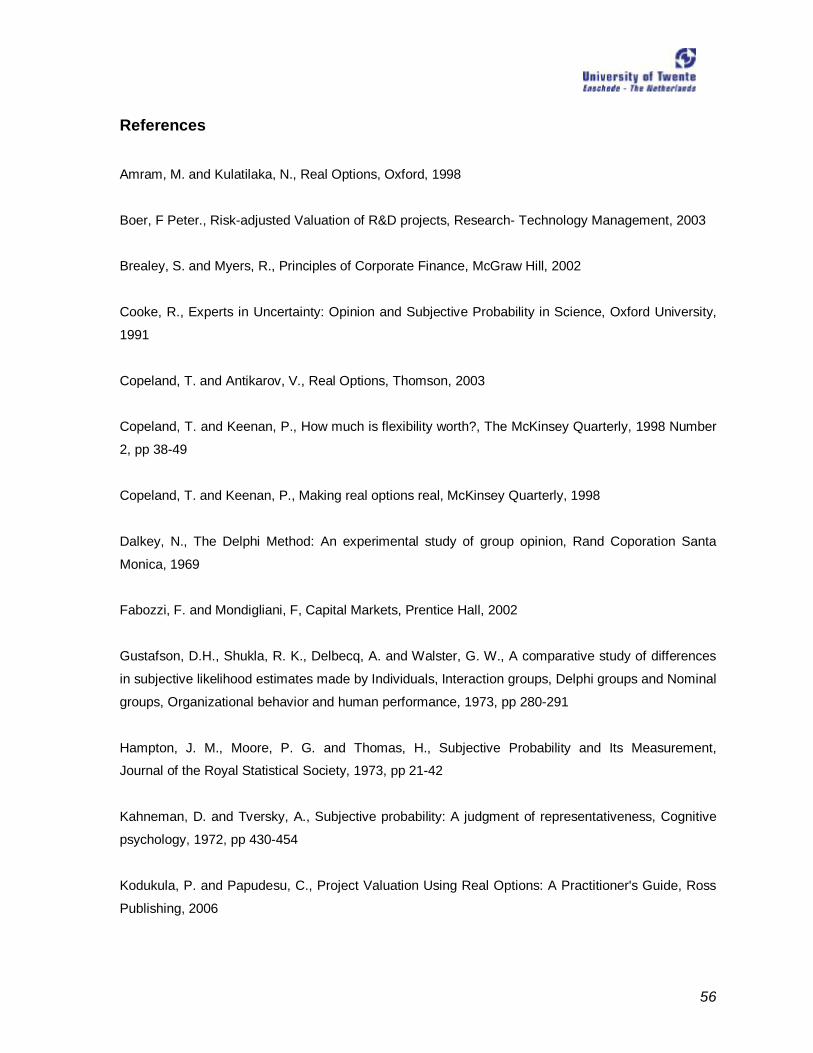
56

References

Amram, M. and Kulatilaka, N., Real Options, Oxford, 1998

Boer, F Peter., Risk-adjusted Valuation of R&D projects, Research- Technology Management, 2003

Brealey, S. and Myers, R., Principles of Corporate Finance, McGraw Hill, 2002

Cooke, R., Experts in Uncertainty: Opinion and Subjective Probability in Science, Oxford University,

1991

Copeland, T. and Antikarov, V., Real Options, Thomson, 2003

Copeland, T. and Keenan, P., How much is flexibility worth?, The McKinsey Quarterly, 1998 Number

2, pp 38-49

Copeland, T. and Keenan, P., Making real options real, McKinsey Quarterly, 1998

Dalkey, N., The Delphi Method: An experimental study of group opinion, Rand Coporation Santa

Monica, 1969

Fabozzi, F. and Mondigliani, F, Capital Markets, Prentice Hall, 2002

Gustafson, D.H., Shukla, R. K., Delbecq, A. and Walster, G. W., A comparative study of differences

in subjective likelihood estimates made by Individuals, Interaction groups, Delphi groups and Nominal

groups, Organizational behavior and human performance, 1973, pp 280-291

Hampton, J. M., Moore, P. G. and Thomas, H., Subjective Probability and Its Measurement,

Journal of the Royal Statistical Society, 1973, pp 21-42

Kahneman, D. and Tversky, A., Subjective probability: A judgment of representativeness, Cognitive

psychology, 1972, pp 430-454

Kodukula, P. and Papudesu, C., Project Valuation Using Real Options: A Practitioner's Guide, Ross

Publishing, 2006

57

Lint, O., Retrospective Insights from real options in R&D, working paper 2000, ECIS

Luehrman, T., Investment opportunities as real options: Getting started on the numbers, Harvard

Business Review (July-August) 1998, pp 51–67

Margolis, D., Probabilistic Approaches: Scenario Analysis. Decision Trees and Simulations, 2003

Rubenstein, A. and Schroder, H., Managerial differences in assessing probabilities of technical

success for R&D projects, Management science, 1977, pp 137-148

Savage, L.J., The foundations of statistics, New York Wiley, 1954

Taylor, D., Berry, P. and Block, C., Does Group Participation When Using Brainstorming Facilitate or

Inhibit Creative Thinking?, Administrative Science Quarterly, 1958

Trigeorgis, L., Real options in Capital Investment: Models, Strategies, and Applications,

Praeger Publishers, 1995

Van De Ven, A. and Delbecq, A., Nominal versus Interacting Group Processes for Committee

Decision-Making Effectiveness, The Academy of Management Journal, 1971

Van De Ven, A. and Delbecq, A., The Effectiveness of Nominal, Delphi, and Interacting Group

Decision Making Processes, The Academy of Management Journal, 1974, pp 605-621

Van Putten, A. and MacMillan, I., Making real options really work, Harvard Business Review,

December 2004, pp 134-141

Winkler, R., The Assessment of Prior Distributions in Bayesian Analysis, Journal of the American

Statistical Association, 1967, pp 775-800.

Documents

Analysis of the tool for the valuation of R&D projectsessay.utwente.nl/58103/1/scriptie_W_Chung.pdf · · 2011-08-28Analysis of the tool for the valuation of R&D projects ... This