ALMA MATER STUDIORUM – UNIVERSITA’ DI BOLOGNA

Scuola di Scienze

Laurea Magistrale in Fisica

Analysis of the scale effect in different computed

tomography systems on the evaluation of bone

tissue parameters

Tesi di laurea di: Relatore:

ANTONELLA BIANCULLI Prof.ssa MARIA PIA MORIGI

Correlatore:

Dott. FABIO BARUFFALDI

Anno Accademico 2015/2016

Di nuovo a Te, Nonna

questa volta forse di più…

…perché Ovunque tu sia,

io so Amare fin lì!

ABSTRACT

Tra le patologie ossee attualmente riconosciute, l’osteoporosi ricopre il

ruolo di protagonista data le sua diffusione globale e la multifattorialità

delle cause che ne provocano la comparsa. Essa è caratterizzata da una

diminuzione quantitativa della massa ossea e da alterazioni qualitative

della micro-architettura del tessuto osseo con conseguente aumento

della fragilità di quest’ultimo e relativo rischio di frattura. In campo

medico-scientifico l’imaging con raggi X, in particolare quello

tomografico, da decenni offre un ottimo supporto per la

caratterizzazione ossea; nello specifico la microtomografia, definita

attualmente come “gold-standard” data la sua elevata risoluzione

spaziale, fornisce preziose indicazioni sulla struttura trabecolare e

corticale del tessuto. Tuttavia la micro-CT è applicabile solo in-vitro,

per cui l’obiettivo di questo lavoro di tesi è quello di verificare se e in

che modo una diversa metodica di imaging, quale la cone-beam CT

(applicabile invece in-vivo), possa fornire analoghi risultati, pur

essendo caratterizzata da risoluzioni spaziali più basse. L’elaborazione

delle immagini tomografiche, finalizzata all’analisi dei più importanti

parametri morfostrutturali del tessuto osseo, prevede la segmentazione

delle stesse con la definizione di una soglia ad hoc.

I risultati ottenuti nel corso della tesi, svolta presso il Laboratorio di

Tecnologia Medica dell’Istituto Ortopedico Rizzoli di Bologna,

mostrano una buona correlazione tra le due metodiche quando si

analizzano campioni definiti “ideali”, poiché caratterizzati da piccole

porzioni di tessuto osseo di un solo tipo (trabecolare o corticale),

incluso in PMMA, e si utilizza una soglia fissa per la segmentazione

delle immagini. Diversamente, in casi “reali” (vertebre umane

scansionate in aria) la stessa correlazione non è definita e in particolare

è da escludere l’utilizzo di una soglia fissa per la segmentazione delle

immagini.

CONTENTS

INTRODUCTION ............................................ 1

CHAPTER 1

- Bone Tissue characterization -

1.1 Structure of bone.............................................................. 4

1.2 Biology of bone tissue ...................................................... 5

1.3 Osteogenesis ...................................................................... 8

1.4 Bone structural organisation ........................................ 11

1.4.1 Types of bone ..................................................... 13

1.5 Bone turnover and development .................................. 14

1.5.1 Bone resorption .................................................. 14

1.5.2 Bone remodelling ............................................... 14

1.6 Bone disease .................................................................... 15

CHAPTER 2

- Imaging Techniques of Bone and its structures -

2.1 X-ray radiation .............................................................. 18

2.2 Computed Tomography ................................................ 24

2.2.1 CT Reconstruction Algorithms ............................... 27

2.2.2 CT Imaging Techniques ......................................... 30

2.2.2.1 Cone Beam Computed Tomography.......... 31

2.2.2.2 Micro-CT .................................................... 32

2.2.2.3 Quantitative Computed Tomography......... 33

2.2.2.4 Single-photon emission computed

Tomograph ............................................... 34

2.2.2.5 Positron emission Tomography ................. 34

CHAPTER 3

- Analysis of structural and densitometric parameters

of bone -

3.1 Osteoporosis ................................................................... 36

3.2 Bone Density ................................................................... 37

3.3 Hounsfield Unit Scale .................................................... 39

3.4 Structural parameters of bone ..................................... 40

3.5 Bone Quality ................................................................... 48

CHAPTER 4

- Experimental tests at the Laboratory of Medical

Technology of “Rizzoli Orthopedic Institute” -

4.1 Aim of thesis ................................................................... 50

4.2 State of the art ................................................................ 50

4.3 Materials and Methods ................................................. 52

4.3.1 Bone Samples .......................................................... 52

4.3.2 Tomographic Imaging Methods ............................. 55

4.3.3 Image Acquisition .................................................. 59

4.3.4 Image Reconstruction ............................................. 60

4.3.5 Image Registration ................................................. 61

4.3.6 Validation of an optimal threshold for image

segmentation .......................................................... 64

4.3.7 Image Segmentation and Calculation of the

Histomorphometric Parameters ............................. 65

4.4 Statistical Analysis ......................................................... 68

CHAPTER 5

- Analysis of Results -

5.1 Defining the optimal threshold value for SkyScan 1176

micro-CT scanner ......................................................... 70

5.2 Analysis of measurements performed on Sample type 1

............................................................................................... 72

5.3 Analysis of measurements performed on Sample type 2

............................................................................................... 76

5.4 Analysis of measurements performed on Sample type 3

............................................................................................... 78

CHAPTER 6

- Discussion of Results -

6.1 Considerations about the measurements performed on

the 3 types of Sample .................................................... 82

6.2 Future Developments .................................................... 84

REFERENCES ............................................... 86

ACKNOWLEDGMENTS .............................. 91

1

INTRODUCTION

The present thesis describes the results of the research work performed

at the Laboratory of Medical Technology of Rizzoli Orthopedic

Institute.

In recent decades, an issue that affects the medical-scientific studies of

orthopedic character, through medical imaging, is undoubtedly inherent

in the osteoporotic disease. Osteoporosis is a systemic disorder

characterized by a quantitative decrease of bone mass and qualitative

alterations of the micro-architecture of the bone tissue, which

predispose to enhanced bone fragility resulting in an increased risk of

fractures. The vertebrae and limb bones are the locations of the human

body most affected and more susceptible to fracture. The fracture is

realized when the load that the bone must support exceeds its capacity

for resistance. Osteoporosis is defined as the most frequent metabolic

disease of the skeleton and it occurs mainly in women in post-

menopausal stage.

The main purpose of this thesis is to compare, through two different

methods of tomographic imaging (micro-CT and cone beam CT with

different spatial resolutions), the morpho-structural parameters

characterizing the bone tissue, with a focus on cancellous bone. In

particular, the aim is to investigate if and how the structural parameters

concerning the bone tissue, calculated with the first method (taken as

reference standard) can also be estimated from the other one.

2

The thesis is divided into six chapters. The first chapter concerns the

description of bone human skeleton with its structural organization and

its biology, while in the second chapter attention focuses on the most

used bone imaging techniques and in particular on Computed

Tomography. In the third chapter the main morphometric parameters,

characterizing the bone micro-architecture, are described while in the

fourth chapter the materials and the methods used for the purposes of

the study are presented. The thesis concludes with the fifth chapter in

which the obtained results are analyzed and plotted and with the sixth

chapter in which the last considerations are done laying the foundations

of what could be the future development of the conducted work.

3

4

CHAPTER 1

Bone Tissue characterization

1.1. Structure of bone tissue

The human skeleton consists of 206 bones. At birth, it is composed of

270 bones, but many of them fuse together as a child grows up. The

main constituent of the skeleton is bone and its fundamentals functions

are to provide support, to give our bodies’ shape, to provide protection

to other systems and organs of the body, to provide attachments for

muscles, to create movement and to produce red blood cells.

The skeletal system includes also connective tissue that differs from

bone because this latter has characteristics of rigidity and hardness. The

human skeleton can be divided into the axial skeleton and the

appendicular skeleton.

The axial skeleton is formed by about 80 bones: the vertebral column

(32-34 bones), the rib cage (12 pairs of ribs and the sternum), the skull

(22 bones) and other associated bones. It maintains the upright posture

of humans. The appendicular skeleton, connected to the axial skeleton,

is formed by 126 bones and in particular by the shoulder girdle, the

pelvic girdle and the bones of the upper and lower limbs. Their

functions are to allow to walk and to protect the major organs of

digestion, excretion and reproduction.

Anatomical differences between human males and females are strongly

marked in some soft tissue areas, but they tend to be limited in the

skeleton. The human skeleton hasn’t sexual different shapes as that of

many other primate species, but delicate differences between genders

in the morphology of the skull, dentition, long bones, and pelvis are

exhibited across human populations. In general, female skeletal

5

elements appear to be smaller and less robust than corresponding male

elements within a given population.

Fig. 1- A anterior and posterior view of the human skeletal system.

1.2. Biology of bone tissue

Bone is a mineralized connective tissue that is characterized by four

types of cells: osteoblasts, bone lining cells, osteocytes, and osteoclasts

(Buckwalter, Glimcher, Cooper, & Recker, 1996).

Osteoblasts are cuboidal cells that are placed along the bone surface

comprising 4–6% of the total present bone cells and are mainly known

for their bone forming function. These cells show morphological

characteristics of protein synthesizing cells, including abundant rough

endoplasmic reticulum and prominent Golgi apparatus (Florencio-Silva

6

et al., 2015). As polarized cells, the osteoblasts secrete, as different

specific proteins, the osteoid toward the bone matrix. Osteoid is the

organic portion, initially unmineralized, of the bone matrix that forms

prior to the maturation of bone tissue.

The synthesis of bone matrix by osteoblasts comes in two main steps:

deposition of organic matrix and its subsequent mineralization. In the

first step, the osteoblasts secrete collagen proteins, mainly type I

collagen, non-collagen proteins and proteoglycan including decorin and

biglycan, which form the organic matrix. Thereafter, mineralization of

bone matrix splits into two phases: the vesicular and the fibrillar phases

(Anderson, 2003). The vesicular phase takes place when portions with

a flexible diameter with a range from 30 to 200 nm, called matrix

vesicles, are liberated from the apical membrane domain of the

osteoblasts into the new formed bone matrix in which they bind to

proteoglycans and other organic components. Given their negative

charge, the sulphated proteoglycans immobilize calcium ions that are

stored within the matrix vesicles (Yoshiko, Candeliere, Maeda, &

Aubin, 2007). When osteoblasts secrete enzymes that deteriorate the

proteoglycans, the calcium ions are released from the proteoglycans and

cross the calcium channels displayed in the matrix vesicles membrane.

Furthermore, phosphates are degraded by the ALP secreted by

osteoblasts that release phosphate ions inside the matrix vesicles. Then,

the phosphate and calcium ions contents the vesicles nucleate, forming

the hydroxyapatite crystals (Florencio-Silva et al., 2015). The fibrillar

phase takes place when the supersaturation of calcium and phosphate

ions inside the matrix vesicles conducts to the rupture of these structures

and the hydroxyapatite crystals spread to the surrounding matrix.

Osteoblasts become mature and, at this moment, it can undergo

apoptosis or become osteocytes or bone lining cells.

7

Osteoclasts are differentiated multinucleated cells, which originate

from mononuclear cells of the hematopoietic stem cell lineage, under

the influence of several factors that promote the activation of

transcription factors and gene expression. They are responsible for the

breakdown of bones. The breakdown of bone is very important in bone

health because it allows for bone remodelling. The osteoclast

disassembles and digests the composite of hydrated protein and mineral

at a molecular level by secreting acid and a collagenase; this process is

named bone resorption. In addition to its main function, the process also

helps regulate the level of blood calcium. Osteoclasts are vital to the

process of bone growth, the rebuilding of bone, and the bone’s ability

to repair itself.

Osteocytes, which comprise 90–95% of the total bone cells, are the

most abundant and long-lived cells, with a half-life of about 25 years

(Franz-Odendaal, Hall, & Witten, 2006). The cell body varies from 5 to

20 micrometers in diameter and contain 40-60 cell processes per cell,

with a cell-to-cell distance between 20-30 micrometers. Different from

osteoblasts and osteoclasts, which have been defined mainly for their

core functions during bone formation and bone resorption, osteocytes

were initially defined by their morphology and location. With the

development of new technologies such as the identification of

osteocyte-specific markers or new techniques for bone cell isolation, it

has been recognized that these cells play numerous important functions

in bone. When osteoblasts become trapped in the matrix that they

secrete, they become osteocytes. Osteocytes are networked to each

other via long cytoplasmic extensions that occupy tiny canals called

canaliculi, which are used for exchange of nutrients and waste through

gap junctions. They are able to molecular synthesis and modification,

as transmission of signals over long distances, in a way similar to the

8

nervous system. Osteocytes contain glutamate transporters that produce

nerve growth factors after bone fracture. When osteocytes are

experimentally destroyed, the bones show a significant increase in bone

resorption, decreased bone formation, trabecular bone loss, and loss of

response to unloading (Noble, 2008). The osteocyte is an important

regulator of bone mass and a key endocrine regulator of phosphate

metabolism.

Bone-lining cells are inactive flat-shaped osteoblasts that cover the

bone surfaces, where neither bone resorption nor bone formation

occurs. Bone lining cells functions are not completely understood, but

it has been shown that these cells allow the direct interaction between

osteoclasts and bone matrix and participate in osteoclasts

differentiation. They allow the osteoclasts access to mineralized tissue.

Bone-lining cells occupy the majority of the adult bone surface and they

are responsible for the immediate release of calcium in the bone if

calcium in the blood is too low (Cowin & Telega, 2003).

1.3. Osteogenesis

There are two modes of bone formation, called also osteogenesis, and

both involve the transformation of a pre-existing mesenchymal tissue

into bone tissue. This direct conversion is called intramembranous

ossification. This process occurs initially in the bones of the skull. In

other cases, the mesenchymal cells differentiate into cartilage, and this

cartilage is later replaced by bone. The process by which a cartilage

intermediate is formed and replaced by bone cells is called

endochondral ossification.

The Intramembranous ossification is the process responsible for the

formation of the flat bones of the skull. During intramembranous

ossification in the skull, neural crest-derived mesenchymal cells grow

9

rapidly and condense into compact nodules. Some of these develop into

capillaries; others change their shape to become osteoblasts, committed

bone precursor cells (Fig.2-A). The osteoblasts secrete a collagen-

proteoglycan matrix that is able to attach calcium salts: the prebone

(osteoid) matrix becomes calcified. In most cases, osteoblasts are

separated from the region of calcification by a layer of the osteoid

matrix they secrete. As calcification proceeds, bony spicules radiate out

from the region where ossification began (Fig.2-B). Furthermore, the

entire region of calcified spicules becomes surrounded by compact

mesenchymal cells that characterize the periosteum (a membrane that

surrounds the bone). The cells on the inner surface of the periosteum

also become osteoblasts and deposit osteoid matrix parallel to that of

the existing spicules. In this manner, many layers of bone are formed

(Gilbert SF. Developmental Biology., 2000).

Fig.2 - Schematic diagram of intramembranous ossification. (A) Mesenchymal cells

condense to produce osteoblasts, which deposit osteoid matrix. These osteoblasts

become arrayed along the calcified region of the matrix. Osteoblasts that are

trapped within the bone matrix become osteocytes. (B) An example of

intramembranous ossification forming the turtle shell.

10

Endochondral ossification involves the formation of cartilage tissue

from aggregated mesenchymal cells, and the subsequent replacement of

cartilage tissue by bone (Horton W A., 1990). It is an essential process

during the rudimentary formation of long bones, the growth of the

length of long bones, and the natural restoring of bone fractures. The

mechanism is very laborious with the implication of many factors that

are beyond my thesis, so Fig. 3 explains a schematic diagram of

endochondral ossification.

Fig. 3 - Schematic representation of endochondral ossification process. A, B)

Mesenchymal cells condense and differentiate into chondrocytes to form the

cartilaginous model of the bone. (C) Chondrocytes in the center of the shaft undergo

hypertrophy and apoptosis while they change and mineralize their extracellular

matrix. Their deaths allow blood vessels to enter. (D, E) Blood vessels bring in

osteoblasts, which bind to the degenerating cartilaginous matrix and deposit bone

matrix. (F-H) Bone formation and growth consist of ordered arrays of proliferating,

hypertrophic, and mineralizing chondrocytes. Secondary ossification centres also

form as blood vessels enter near the tips of the bone.

11

1.4. Bone structural organisation

To appreciate the mechanical properties of bone material, it is important

to investigate the various levels of hierarchical structural organization

of bone. These levels and structures are:

• the macrostructure: cancellous and cortical bone;

• the microstructure (from 10 to 500 μm): Haversian systems,

osteons, single trabeculae;

• the sub-microstructure (1–10 μm): lamellae;

• the nanostructure (from a few hundred nanometers to 1 μm):

fibrillar collagen and embedded mineral;

• the sub-nanostructure (a few hundred nanometers): molecular

structure of constituent elements, such as mineral, collagen, and non-

collagenous organic proteins.

Bone is not a uniformly solid material. Human skeleton is composed of

two types of osseous tissues whose difference consists in their structure

and distribution and that are designed to perform different functions.

The hard outer layer of bones is constituted by cortical bone also called

compact bone. The word cortical refers to the exterior (cortex) layer.

The hard exterior layer gives bone its smooth, white, and solid

appearance; it is much denser than cancellous bone, stronger and stiffer.

Cortical bone provides about 80% of the weight of a human skeleton.

At microscope cortical bone consists of multiple columns, each called

an osteon. Each column is structured of layers of osteoblasts and

osteocytes around a central canal called the Haversian canal. Around it,

there are concentric rings (lamellae) of matrix. Volkmann's canals

connect the osteons together. Between the rings of matrix, the bone cells

(osteocytes) are placed in spaces called lacunae. Small channels

(canaliculi) diffuse from the lacunae to the osteonic (Haversian) canal

12

to supply passageways through the hard matrix. The osteonic canals

contain blood vessels that are parallel to the long axis of the bone. These

blood vessels interconnect, through perforating canals, with vessels on

the surface of the bone.

Fig. 4 – (a) Microscopic Anatomy of Bone. (b) Canaliculi connect lacunae to each

other and the central canal. (c) Lacunae, small cavities that contain osteocytes

The major functions of cortical bone are to support the whole body

weight, to protect organs, to provide levers for movement, to store and

release calcium.

Cancellous bone is also called trabecular bone or spongy bone.

Compared to cortical bone, it has a higher surface area but is less dense,

13

softer, weaker, and less stiff. It typically occurs at the ends of long

bones, proximal to articulations and within the interior of vertebrae.

Microscopically, cancellous bone consists of plates (trabeculae) and

other irregular cavities that contain bone marrow. The trabeculae of

spongy bone succeed the lines of stress and can realign if the direction

of stress changes. It may appear that the trabeculae are arranged in an

irregular manner, but they are organized to provide maximum strength.

Thanks to its greater surface area, cancellous bone is ideal for metabolic

activity, e.g. exchange of calcium ions.

1.4.1. Types of bone

There are five types of bones in the human body classified by shape:

long, short, flat, irregular, and sesamoid. Long bones are composed by

a shaft, the diaphysis, which is much longer than its width, and by an

epiphysis, a rounded head at the end of the shaft. They are made up

mostly of compact bone, with lesser amounts of marrow, located within

the medullary cavity, and cancellous bone. Most bones of the limbs,

including fingers and toes, are long bones. Short bones are irregularly

cube-shaped, and have only a thin layer of compact bone surrounding a

spongy interior. An example of short bones are the wrist and ankle. Flat

bones are thin, generally curved, with two parallel layers of compact

bones and, in the middle, a layer of spongy bone. Most of the bones of

the skull are flat bones, as is the sternum. Sesamoid bones are bones

implanted in tendons. Examples of sesamoid bones are the patella and

the pisiform. Irregular bones do not fit into the categories mentioned

until now. They consist of thin layers of external compact bone with a

spongy bone within. Their shapes are irregular and complex. The bones

of the spine, pelvis, and some bones of the skull are irregular bones.

14

1.5. Bone turnover and development

1.5.1. Bone resorption

Bone resorption is a process consisting in the breakdown of bone by

specialized cells known as osteoclasts. It occurs on a continual level

inside the body, with the destroyed bone replaced by new bone growth.

Osteoclasts work by attaching themselves to individual bone cells and

secreting compounds to break the cells, with subsequent release of their

mineral contents. The minerals enter the bloodstream, where they are

processed for recycling of new bone or eliminated with other bodily

wastes. Osteoclasts break bone consequently to inflammation, disease

and injury, removing damaged bone to allow it to be replaced with new

bone. In cases where bone resorption becomes accelerated, bone is

broken down faster than it can be renewed. The bone becomes more

porous and fragile, facilitating the risk of fractures.

1.5.2. Bone remodeling

Bone remodeling, called also bone metabolism, is an important process

that occurs throughout a person’s lifetime; ossification and resorption

work together to reshape the skeleton during growth, to maintain

calcium levels in the body and to repair micro-fractures caused by

quotidian stress. During the bone remodeling process, bone-making

cells called osteoblasts deposit new bone and osteoclasts absorb the old

bone. The remodelling has both positive and negative effects on bone

tissue quality. It allows removing micro-damage, replacing dead and

hypermineralized bone and adapting the microarchitecture to local

stress. However, remodelling may also perforate or remove trabeculae,

increase cortical bone porosity, decrease cortical width and possibly

reduce bone strength.

15

1.6. Bone disease

Bone disease is a condition that injures the skeleton, makes bones weak

and prone to fractures. Despite strong bones are structured in childhood,

people, in every part of their life, can improve their bone health. The

most common bone disease is osteoporosis, which is characterized by

low bone mass and deterioration of bone structure. Low bone mass is

when bones lose minerals, like calcium, and as consequence, bones

become weak and fracture easily. Calcium is an essential mineral

needed by the body to build strong bones and to keep them strong

throughout the life. Calcium is also needed for other purposes, such as

muscle contraction. Almost all calcium (99 percent) is stored in the

bones. The remaining one percent circulates in the body. 'Osteoporosis'

literally means 'porous bones' and is often referred to as the 'fragile bone

disease' in an increased risk of fractures of the hip, spine, and wrist with

consequences for the bone mechanics. Osteoporosis is often called a

"silent" disease because it has no discernible symptoms until there is a

bone fracture.

Many factors lead to fractures: age, heredity, body weight, diseases,

lifestyle, frailty, and amount of trauma all play important roles.

Osteoporosis can be prevented, as well as diagnosed and treated.

Fractures to weak bones typically occur from falling or other common

accidents.

16

Fig. 5 - Diagram illustrating the course of bone gain and loss throughout life and

fracture risk. Horizontal dotted line represents the level below which structural

failures or fractures are likely to occur. This level is reached earlier in women than

in men because of the differences in the magnitude of the age-related bone loss. In

both sexes, level is reached earlier in those who accumulate less bone (peak bone

mass) during growth (Clifford J. Rosen, Roger Bouillon, Juliet E. Compston, 2013).

The incidence of osteoporotic fractures is very high: in the USA, about

45% of postmenopausal women have low bone density. The lifetime

risk of a fracture of the hip, spine or forearm is 40% in white women

and 13% in white men. African-Americans have fewer fractures than

people of other races. Worldwide the rates of osteoporosis are variable,

but in every country, age is one of the most important risk factors. As

more people live longer lives, the number of those with osteoporosis

will also increase (Melton, 1992).

17

Fig. 6 - Trabecular bone structure in the lower spine of a young adult compared to

an osteoporotic elderly adult.

Other bone diseases include Paget's disease and osteogenesis

imperfecta. Paget's disease affects older men and women, and causes

skeletal deformities and fractures. Osteogenesis imperfecta is an

inherited disorder that causes brittle bones and frequent fractures in

children.

18

CHAPTER 2

Imaging Techniques of Bone and its structures

Medical imaging is the technique and process that allows to have visual

representations of the interior of a body for clinical analysis and medical

intervention, for example a representation of the function of some

organs or tissue. Currently, this ability to get information about the

human body has many clinical applications. In the last decades,

different sorts of medical imaging have been developed, each with its

own advantages and disadvantages. The most used is imaging with X-

ray based methods, but not less relief, especially in recent years, has

been attributed to other types of medical imaging such as magnetic

resonance imaging (MRI) and ultrasound imaging. The success of these

techniques is due to the fact that they operate without ionizing radiation.

MRI uses strong magnetic fields, which do not produce known

irreversible biological effects in humans. Diagnostic ultrasound

systems use high-frequency sound waves to create images of soft tissue

and internal body organs.

2.1. X-ray radiation

X-radiation is a form of electromagnetic radiation with a wavelength in

the range from UV rays (longer) and Gamma rays (shorter). The term

“X-radiation” was first coined by its discover, Wilhelm Röntgen, who

named it in this way to connote an unknown type of radiation.

19

Due to their penetrating ability, X-rays are largely used to image the

inside of objects, e.g. in medical radiography.

X-ray photons transport energy sufficient to ionize atoms and

disintegrate molecular bonds: this makes them a type of ionizing

radiation. A very high radiation dose delivered in a short time generates

radiation sickness, while lower doses can give an increased risk of

cancer induced by radiation. In medical imaging this risk is generally

greatly outweighed by the benefits of the examination. The ionizing

capability of X-rays can be utilized in cancer treatment to kill malignant

cells using radiation therapy. X-rays can traverse relatively thick

objects without being much absorbed or scattered. For this reason. X-

rays are widely used to image the inside of opaque objects and the

“penetration depth” varies by several orders of magnitude over the X-

ray spectrum. X-rays interact with matter in different ways:

photoabsorption, Compton scattering, Rayleigh scattering, pair

production. The strength of these interactions depends on the energy of

the X-rays and the composition of the material. Photoabsorption or

photoelectric absorption is the dominant interaction mechanism in the

soft X-ray regime and for the lower hard X-ray energies. At higher

energies, Compton scattering dominates (Jerrold T. Bushberg, J.

Anthony Seibert, Edwin M. Leidholdt Jr., 2002).

The scheme of an X-ray tube is represented in Fig. 7. A high voltage is

needed to produce the required kinetic energy of the electrons emitted

from the cathode. When these electrons bombard the heavy metal atoms

of the anodic target, they interact with these atoms and transfer their

kinetic energy to the target. In particular, the electrons interact with the

outer-shell electrons of the target atoms elevating them to a higher

energy level (excited). At this point, the outer-shell electrons

immediately drop back to their normal energy state emitting infrared

20

radiation. The constant excitation and re-stabilization of outer-shell

electrons causes heat inside the anodes of X-ray tubes. Generally, more

than 99% of the kinetic energy of the accelerated electrons is converted

to thermal energy, instead less than 1% is available for the production

of X-radiation (Dendy, Heaton, & Cameron, 2001).

Fig. 7 – Essential features of a simple, stationary anode X-ray tube. For simplicity,

only X-ray photons passing through the window are shown. In practice, they are

emitted in all directions.

A typical X-ray spectrum is shown in Fig. 8 in which the two curves

represent two different accelerating voltages. The X-ray spectrum can

be divided in two parts: (a) a continuous background, and (b) a series

of sharp peaks.

21

Fig. 8 Typical X-Ray spectrum with different voltages.

The electromagnetic attraction of the nuclei of the target material

determines the electron slowdown and the consequent production of the

so-called bremsstrahlung radiation. An X-ray photon with the minimum

wavelength and therefore the maximum energy and frequency is

produced when an electron is stopped by just one nucleus. The rest of

the continuous curve in Fig. 8 is due to electrons that lose only part of

their energy during collisions with many nuclei

Minimum X ray wavelength (λ) = hc/eV

where V is the accelerating voltage and c the velocity of light.

The peaks on the spectrum are characteristic of the particular target

material. The bombarding electrons are able to ionize the target atoms

by removing electrons from the inner shells. When this happens an

electron from an outer energy level fills the vacancy emitting a photon

of a definite wavelength, thus giving a sharp peak on the spectrum

(Keith Gibbs, 2006).

22

The efficiency of X-ray production is independent of the tube current,

but it increases with increasing electron energy. At 60 keV, only 0.5%

of the electron kinetic energy is converted to X-rays; at 120 MeV, it is

70% (Fig.9) (Poludniowski, Landry, DeBlois, Evans, & Verhaegen,

2009).

Fig.9 - Dependence of the output of an X-ray tube on applied voltage.

As already previously said, when X-rays are directed on an object, some

photons interact with the particles of the matter and their energy can be

absorbed or scattered. This absorption and scattering is called

attenuation. Other photons proceed through the object without

interacting with any of the material's particles. The number of photons

transmitted depends on the thickness, density and atomic number of the

material. If the photons have the same energy, they travel however at

different distances within a material relying on the probability of their

encounter with one or more of the particles of the matter and the

modality of the interaction. Greater the distance traveled, greater the

probability of collision with the particles; the number of photons

23

reaching a specific point within the matter decreases exponentially with

distance traveled.

Fig. 10 - Dependence of X-ray radiation intensity on absorber thickness in case of

a monochromatic X-ray beam (NDT Resource Center)

The formula that describes the curve shown in Fig. 10 is:

𝐼 = 𝐼0𝑒−𝜇𝑥

where:

𝜇 is the linear attenuation coefficient

𝐼 is the intensity of photons transmitted across some distance x

𝐼0 is the initial intensity of photons

𝑥 is the distance traveled

The linear attenuation coefficient (µ) depends on the atomic number of

the material, the density of the medium and the energy of the beam.

24

2.2. Computed Tomography

Among many medical imaging techniques, my thesis focuses on

Computed Tomography (CT) that is a diagnostic imaging modality used

to produce detailed images of internal organs, bones, soft tissue and

blood vessels. In particular, Computer Axial Tomography (CAT)

generates an image (CAT scan) of the tissue density in a “slice” as thin

as 1 to 10 mm in thickness through the patient's body. The cross-

sectional images generated during a CT scan can be reformatted in

multiple planes, three-dimensional images can even generate and after

they can be viewed on a computer monitor, or transferred to electronic

media. Since its introduction in 1972 by Hounsfield, the use of CT has

grown rapidly.

An X-ray source that rotates around the object generates X-ray slice

data; X-ray sensors are positioned on the opposite side of the circle from

the X-ray source. The earliest sensors were scintillation detectors, with

photomultiplier tubes excited by (typically) cesium iodide crystals.

Cesium iodide was replaced during the 1980s by ion chambers

containing high-pressure Xenon gas. The first clinical CT images were

produced at the Atkinson Morley Hospital in London in 1972. The very

first patient examination using CT, offered credible proof of the

effectiveness of the method by detecting a cystic frontal lobe tumor. CT

was immediately and enthusiastically introduced in the medical field by

the medical community and has often been referred as the most

important invention in diagnostic radiology since the discovery of X-

rays. In 1979, Godfrey Hounsfield and Allan Cormack, an engineer and

a physicist, were awarded the Nobel Prize for medicine in recognition

of their outstanding achievements. The EMI scanner (1973) was

designed for brain scanning, and its applications were limited to the

25

head (Fig. 11). The pencil beam employed in the first generation

scanner resulted in poor geometrical utilization of the X-ray beam and

it required long scanning times. In the second-generation scanner, the

X-ray beam was collimated to a 10-degree fan, which circumscribed an

array of 8 to 30 radiation detectors, rather than the previous pencil beam

with only a single detector. Despite the second-generation scanner also

used the translate-rotate mechanical motion, which created many

difficulties, the fan beam, crossing the patient, permitted to obtain

multiple angles with a single translation (Fig.12).

Fig. 11 - Illustration of the scanning Fig.12 - Second-generation CT scanner

sequence in a first-generation CT scanner

There are a limited number of beams (approximately 8 to 30) in a

narrow fan configuration with the same translate-rotate motion used in

first-generation machines. Each linear scan produces several

projections at differing angles, one view for each X-ray beam. The

fastest second-generation CT units could achieve a scanning time of 18

seconds per slice. The image quality was substantially improved.

However, the second-generation units had definite speed limitations

due to the inertia of the heavy X-ray tube and gantry during the

complicated translate rotate motion. To improve speed, third- and

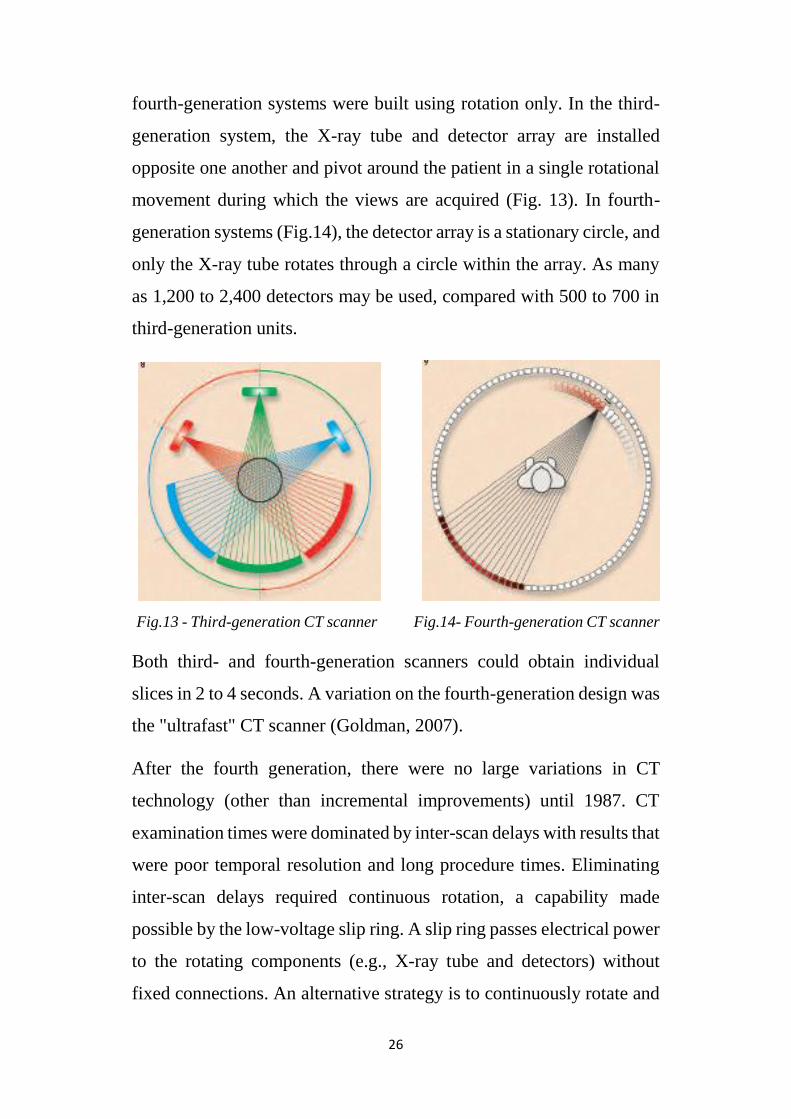
26

fourth-generation systems were built using rotation only. In the third-

generation system, the X-ray tube and detector array are installed

opposite one another and pivot around the patient in a single rotational

movement during which the views are acquired (Fig. 13). In fourth-

generation systems (Fig.14), the detector array is a stationary circle, and

only the X-ray tube rotates through a circle within the array. As many

as 1,200 to 2,400 detectors may be used, compared with 500 to 700 in

third-generation units.

Fig.13 - Third-generation CT scanner Fig.14- Fourth-generation CT scanner

Both third- and fourth-generation scanners could obtain individual

slices in 2 to 4 seconds. A variation on the fourth-generation design was

the "ultrafast" CT scanner (Goldman, 2007).

After the fourth generation, there were no large variations in CT

technology (other than incremental improvements) until 1987. CT

examination times were dominated by inter-scan delays with results that

were poor temporal resolution and long procedure times. Eliminating

inter-scan delays required continuous rotation, a capability made

possible by the low-voltage slip ring. A slip ring passes electrical power

to the rotating components (e.g., X-ray tube and detectors) without

fixed connections. An alternative strategy is to continuously rotate and

27

continuously acquire data as the table (patient) is smoothly moved

though the gantry; the resulting trajectory of the tube and detectors

relative to the patient traces out a helical or spiral path (Fig. 15). This

powerful concept led to the construction of Helical CT (or Spiral CT)

(Goldman, 2007).

However, the basic principles are similar for all techniques: all

reconstructed cross-section images are based on the attenuation

coefficients of the object that is examined.

Fig. 15 - Helical CT. Improved body CT was made possible with advent of helical

CT (or spiral CT). Patient table is moved smoothly through gantry as rotation and

data collection continue. Resulting data form spiral (or helical) path relative to

patient; slices at arbitrary locations may be reconstructed from these data.

Today, most modern hospitals currently use spiral CT scanners and

beam types can be parallel beams, fan-beams, and cone-beams.

2.2.1 CT Reconstruction Algorithms

When talking about reconstruction algorithms, reference is made to four

main methods aimed at computing the slice image given the set of its

views. The first method is hardly workable, but provides a better

28

understanding of the problem. It is based on solving many

simultaneous linear equations. One equation can be written for each

measurement. That is, a particular sample in a particular profile is the

sum of a particular group of pixels in the image. To calculate unknown

variables (i.e., the image pixel values), there must be independent

equations, and therefore N2 measurements, if N×N is the size of the

image.

The second method of CT reconstruction uses iterative techniques to

calculate the final image in a few steps. There are several variations of

this method: the Algebraic Reconstruction Technique (ART), the

Simultaneous Iterative Reconstruction Technique (SIRT), and the

Iterative Least Squares Technique (ILST). The difference between

these methods is given by consequentiality of the corrections: ray-by-

ray, pixel-by-pixel, or simultaneously correcting the entire data set,

respectively. Iterative techniques are generally slow, but they are useful

when better algorithms are not available.

The third method is called filtered backprojection. It is the most

common used algorithm for computed tomography systems. It is a

modification of an older technique, called backprojection or simple

backprojection. Filtered backprojection is a technique to correct the

blurring found in simple backprojection. Each of the one-dimensional

views is convolved with a one-dimensional filter kernel to compose a

set of filtered views. These filtered views are then backprojected to

provide the reconstructed image. In fact, the image produced by filtered

backprojection is identical to the "correct" image when there are an

infinite number of views and an infinite number of points per view.

The fourth method is called Fourier reconstruction. In the spatial

domain,

29

Fig. 16 – Filtered backprojection.

CT reconstruction involves the association between a two-dimensional

image and its set of one-dimensional views. The frequency domain

analysis of this problem is a milestone in CT technology called the

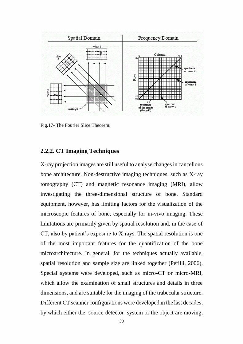
Fourier slice theorem. It describes the relationship between an image

and its views in the frequency domain. In the spatial domain, each view

is found by integrating the image along rays at a particular angle. In the

frequency domain, the spectrum of each view is “one-dimensional”

slice of the two-dimensional image spectrum (Smith, 1999).

30

Fig.17- The Fourier Slice Theorem.

2.2.2. CT Imaging Techniques

X-ray projection images are still useful to analyse changes in cancellous

bone architecture. Non-destructive imaging techniques, such as X-ray

tomography (CT) and magnetic resonance imaging (MRI), allow

investigating the three-dimensional structure of bone. Standard

equipment, however, has limiting factors for the visualization of the

microscopic features of bone, especially for in-vivo imaging. These

limitations are primarily given by spatial resolution and, in the case of

CT, also by patient’s exposure to X-rays. The spatial resolution is one

of the most important features for the quantification of the bone

microarchitecture. In general, for the techniques actually available,

spatial resolution and sample size are linked together (Perilli, 2006).

Special systems were developed, such as micro-CT or micro-MRI,

which allow the examination of small structures and details in three

dimensions, and are suitable for the imaging of the trabecular structure.

Different CT scanner configurations were developed in the last decades,

by which either the source-detector system or the object are moving,

31

the number of detectors are augmented, with the principal aim to reduce

scan-time (Kak, Author, Slaney, Wang, & Reviewer, 2002). Below, a

little summary of typical and most used 3D-imaging procedures is

reported.

2.2.2.1. Cone beam computed tomography

Cone-beam computed tomography (CBCT) is a medical imaging

technique characterized by a CT set-up with cone-beam geometry and

a two-dimensional detector. CBCT has become increasingly important

for treatment planning and diagnosis in implant dentistry and

interventional radiology (IR). It provides sub-millimetre resolution in

images of high diagnostic quality, with brief scanning times (10–70

seconds) and radiation dosages reportedly up to 15 times lower than

those of conventional CT scans (Scarfe, Farman, & Sukovic, 2006).

Cone-beam technology was first introduced in the European market in

1996 by QR s.r.l. (Verona, Italy).

Fig.18- An example of CBCT machine

32

2.2.2.2. Micro-CT

Micro–computed tomography (micro-CT or µCT) has applications both

in medical imaging and in the industrial field. The first X-ray

microtomography system was idealised and built by Jim Elliott in the

early 1980s. The first published X-ray microtomographic images were

reconstructed slices of a small tropical snail, with pixel size about 50

micrometers (Elliott & Dover, 1982). The prefix micro- (symbol µ) is

used to indicate that the pixel size of the cross-sections is in the

micrometer range. In general, the system consists of a microfocus tube,

which generates a cone-beam of X-rays, a rotating specimen holder, on

which the object is positioned and a detector system that acquires the

images. Differently from medical CT, in the micro-CT, the source-

detector system is fixed, while the images are taken with the specimen

rotating on a turntable. Typically, it is used for small animals (in vivo

scanners), biomedical samples, foods, microfossils and other studies for

which minute details are desired. Today, systems with spatial

resolutions in the order of few μm or even better are available

(http://www.skyscan.be (2006)). It is important to say that the spatial

resolution during a scan with a cone-beam geometry is strictly related

to the size of the object in examination.

Fig.19 – An example of Micro-CT device on the market.

33

2.2.2.3. Quantitative Computed Tomography

Quantitative computed tomography (QCT) is a medical technique that

measures bone mineral density (BMD) using a standard X-ray

Computed Tomography (CT) scanner with a standard calibration

capable to convert Hounsfield Units (HU) of the CT image to BMD

values. Quantitative CT scans are primarily used to evaluate bone

mineral density at the lumbar spine and hip. QCT exams are typically

used in the diagnosis and monitoring of osteoporosis. Today, modern

3D QCT uses the ability of CT scanners to rapidly acquire multiple

slices to construct three-dimensional images of the human body. The

use of 3D imaging is fundamental to reduce image acquisition time, to

improve reproducibility and to enable QCT bone density analysis of the

hip (Adams, 2009). An important role, furthermore, is played by

peripheral quantitative computed tomography, that, as the name

implies, is a type of quantitative computed tomography in a peripheral

part of the body such as the forearms or legs and, in particular, the HR-

pQCT (High-Resolution- peripheral quantitative computed

tomography) that is a newly developed in vivo clinical imaging

modality. It can assess the 3D microstructure of cortical and trabecular

bone to evaluate bone’s mechanical properties. (Liu, Saha, & Xu,

2012).

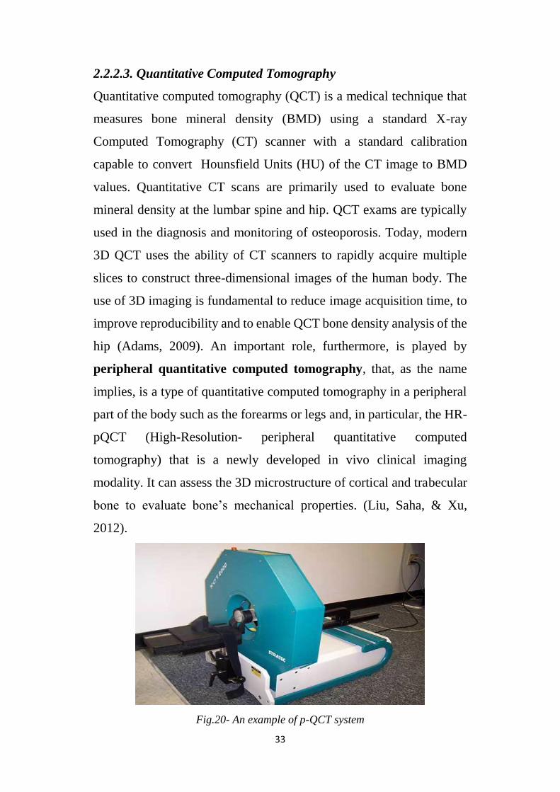
Fig.20- An example of p-QCT system

34

2.2.2.4. Single-photon emission computed tomography

Single-photon emission computed tomography (SPECT) is a method of

computed tomography that uses radionuclides, which emit a single

photon of a given energy. The camera is rotated 180 or 360 degrees

around the patient to capture multiple 2-D images at multiple positions

along the arc. A computer is then used to apply a tomographic

reconstruction algorithm to the multiple projections, yielding a 3-D data

set. It requires delivery of a gamma-emitting radioisotope administrated

to the patient through injection into the bloodstream. It can be used to

provide information about localised function in internal organs, such as

functional cardiac or brain imaging, but at the same time, to

complement any gamma imaging study such as thyroid imaging or bone

scintigraphy. In some cases, a SPECT gamma scanner may be built to

operate with a conventional CT scanner, with co-registration of images.

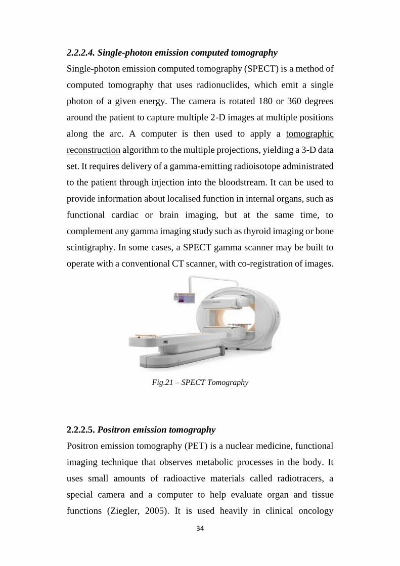
Fig.21 – SPECT Tomography

2.2.2.5. Positron emission tomography

Positron emission tomography (PET) is a nuclear medicine, functional

imaging technique that observes metabolic processes in the body. It

uses small amounts of radioactive materials called radiotracers, a

special camera and a computer to help evaluate organ and tissue

functions (Ziegler, 2005). It is used heavily in clinical oncology

35

(medical imaging of tumors and the search for metastases), but is also

an important research tool to map normal human brain and heart

function. PET scans are increasingly read alongside CT or magnetic

resonance imaging (MRI) scans, because this combination (called "co-

registration") provides both anatomic and metabolic information. PET

imaging, in this way, became most useful; in fact, PET scanners are

now available with integrated high-end multi-detector-row CT scanners

(so-called "PET-CT").

Fig. 22 – PET Tomography

36

CHAPTER 3

Analysis of structural and densitometric

parameters of bone

3.1 Osteoporosis

As mentioned in the Chapter 1, osteoporosis is the most common

metabolic bone disease that affects the entire skeleton, particularly the

cancellous and cortical bone. It occurs mainly in women going through

menopause. In 2001, it was observed that 1 in 2 women and 1 in 5 men

over age 50 in the West, would experience a fracture in their lifetime

(Van Staa, Dennison, Leufkens, & Cooper, 2001). Current data are

even more gruesome, in fact the National Osteoporosis Foundation

(NOF) estimated that in 2010, 10 million Americans are to have

osteoporosis and 34 million more to have low bone mass; furthermore

is expected that the disease will increase to 14 million by 2020 (Cosman

et al., 2014). For this reason, since 1994 the World Health Organization

(WHO) reported that osteoporosis was a global problem and

recommended bone mineral density (BMD) study for early detection of

osteoporosis above all in the postmenopausal population.

Diagnosis of osteoporosis can be made thought radiographs when

multiple fractures are present or when structural abnormalities,

characteristic of the abovementioned disease, appear: in particular, low

bone mass, micro-architectural deterioration of bone tissue and

increased bone fragility. However, the use of visual observation and

interpretation of a radiograph is not sufficient because technical

considerations, such as patient size, exposure and processing factors,

may be inaccurate and influence how dense the bones appear.

37

In the chapter 2 we saw that CT is an imaging technique that shows

human anatomy in cross sections and provides a three-dimensional

dataset that can be used for image reconstruction and analysis in

distinct planes or three-dimensional settings. CT is used to provide not

only morphological information, but also every information about

tissue attenuation and to identify most of bone pathology, from

traumatic lesions to bone neoplasm. Attenuation values can be

extracted from CT data and used to reconstruct images. These

values can also be used to estimate the density of tissues. (Celenk

& Celenk, 2008).

3.2 Bone Density

Bone density (or bone mineral density) is a medical term referring to

the measure of mineral bone per square centimeter in a bone tissue

(Fig.23). Bone density is used in clinical medicine as an indirect

indicator of osteoporosis and fracture risk. BD measurements are most

commonly made because the technique is non-invasive, painless and

involves minimal radiation exposure. In recent studies, many

approaches have been introduced to measure skeletal BD. All the

methods for bone density measurement use a low-intensity beam of X-

rays (or gamma-rays) passing through a patient and a radiation detector

on the opposite side that quantifies how much of the beam is absorbed.

Part of the beam is absorbed by the bone and part by the surrounding

soft tissue. The purpose of each technique is to measure precisely how

much is this difference. There are several types of bone mineral density

tests such as:

Ultrasound

DEXA (Dual Energy X-ray Absorptiometry)

38

SXA (single Energy X-ray Absorptiometry)

PDXA (Peripheral Dual Energy X-ray Absorptiometry)

RA (Radiographic Absorptiometry)

DPA (Dual Photon Absorptiometry)

SPA (Single Photon Absorptiometry)

MRI (Magnetic Resonance Imaging)

QCT (Quantitative Computed Tomography)

Laboratory tests

QCT is considered as the gold standard compared with other

measurements of Bone Density (Guglielmi, Grimston, Fischer, &

Pacifici, 1994). Unlike the others, this technique produces a cross-

sectional or 3-dimensional image from which the bone is measured

directly, independently from the surrounding soft tissue. QCT,

furthermore, allows to measure 100% isolated trabecular bone which is

approximately eight times more metabolically active than cortical

bone (Reinbold, Genant, Reiser, Harris, & Ettinger, 1986). Other

techniques measure the mixture of trabecular bone and the overlying

compact bone.

Fig. 23 – Difference between Normal Bone Density and Low Bone Density in a

vertebra (“Bone Density Scan”).

39

3.3 Hounsfield Unit Scale

To quantify some property of the bone tissue, it is necessary to

determine the standard calibration of the X-ray attenuation. For each

pixel in an image, a numerical value (CT number) is assigned, which is

the average of all the attenuation values contained within the

corresponding voxel. This CT numbers are compared to the attenuation

value of water and displayed on a scale of arbitrary units named

Hounsfield units (HU) scale. In this way, it is possible to define the

linear transformation of the original linear attenuation coefficient

measurement into one in which the radiodensity of distilled water at

standard pressure and temperature (STP) is defined as zero, while the

radiodensity of air at STP is defined as -1000 HU (Celenk & Celenk,

2008).

For a material X with linear attenuation coefficient μx, the

corresponding HU value is given by

HU = 𝜇𝑥− 𝜇𝑤𝑎𝑡𝑒𝑟

𝜇𝑤𝑎𝑡𝑒𝑟−𝜇𝑎𝑖𝑟 x 1000

Where 𝜇𝑤𝑎𝑡𝑒𝑟 and 𝜇𝑎𝑖𝑟 are respectively the linear attenuation

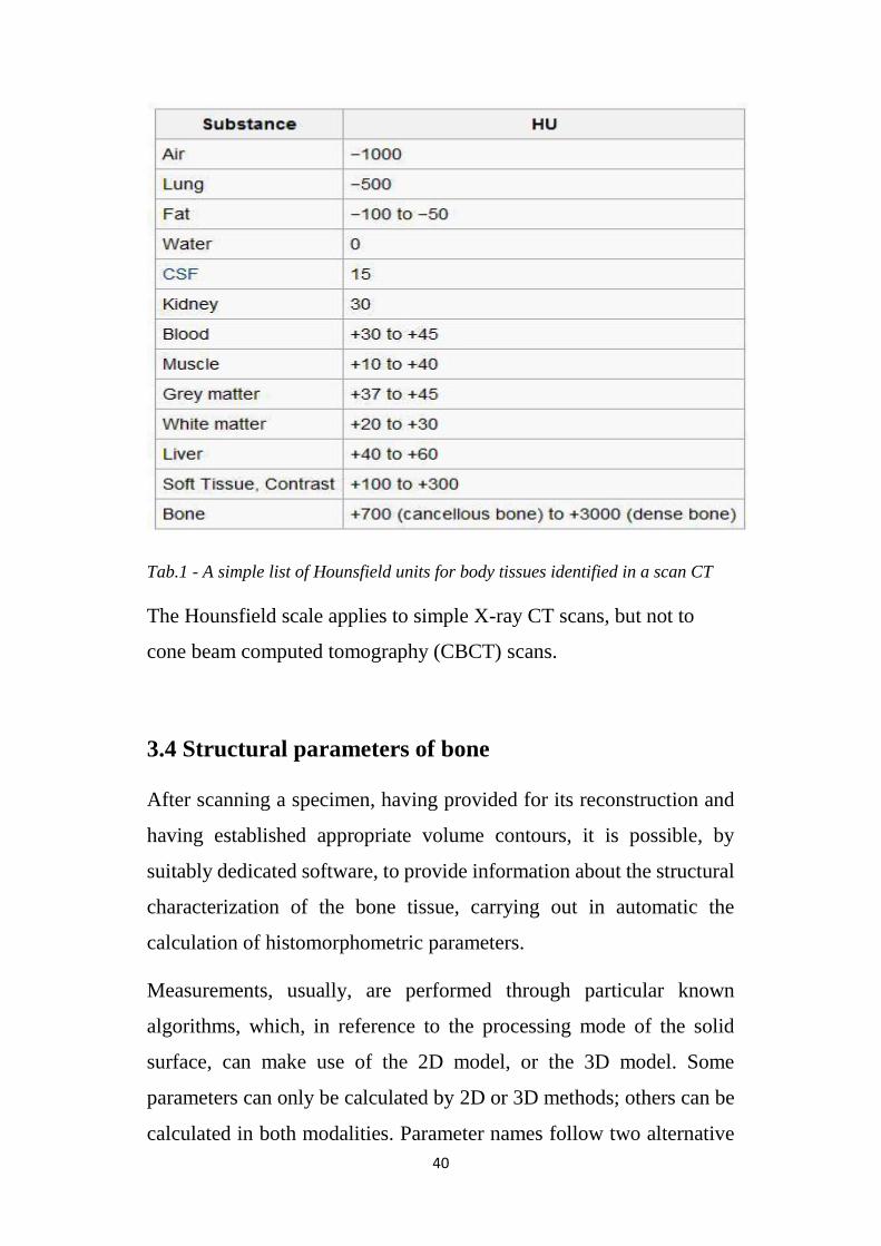
coefficients of water and air. In Tab.1 the HU of common substances.

It is important to underline that the Hounsfield number of a tissue

varies according to the density of the tissue; so the higher the

number, the denser is the tissue and the HU can be used directly to

determine bone quality alterations.

40

Tab.1 - A simple list of Hounsfield units for body tissues identified in a scan CT

The Hounsfield scale applies to simple X-ray CT scans, but not to

cone beam computed tomography (CBCT) scans.

3.4 Structural parameters of bone

After scanning a specimen, having provided for its reconstruction and

having established appropriate volume contours, it is possible, by

suitably dedicated software, to provide information about the structural

characterization of the bone tissue, carrying out in automatic the

calculation of histomorphometric parameters.

Measurements, usually, are performed through particular known

algorithms, which, in reference to the processing mode of the solid

surface, can make use of the 2D model, or the 3D model. Some

parameters can only be calculated by 2D or 3D methods; others can be

calculated in both modalities. Parameter names follow two alternative

41

nomenclatures, “General Scientific” or “Bone ASBMR”, the latter

being based on a paper elaborated by Parfitt in the 1987. Parfitt’s paper

proposed a system of symbols for bone histomorphometry (Parfitt AM,

Drezner MK, Glorieux FH, Kanis JA, Malluche H, Meunier PJ, Ott SM,

1987). All measurements of morphometric parameters in 3D and 2D are

performed on segmented or binarized images. Segmentation, also called

“thresholding”, must be done prior to morphometric analysis (Skyscan,

2005). Following are some of the main parameters, classified according

to nomenclature ASBMR, in reference to the bone tissue structure:

Total Volume (TV), (mm3)

It represents the volume of interest, i.e. the total volume

subjected to analysis, for the selected ROI (region of interest),

including both the spaces occupied by bone material and the

empty spaces. It can be measured both in 2D and in 3D and is

based on a simple count of voxels contained in the selected

volume model.

Bone Volume (BV), (mm3)

It represents that part of the volume of interest occupied only by

solid bone material; it can be calculated in 2D and 3D modes, and

is based on counting voxel only recognized as a solid material.

Percent Bone Volume (BV/TV), (%)

It represents the percentage of the volume occupied by bone

material compared to the total volume considered. It is calculated

both in 2D and 3D, simply by making the ratio of BV and TV

parameters, respectively calculated in two different ways.

42

Bone Surface (BS), (mm2)

It represents the delimiting surface of regions occupied by solid

bone material; the 2D measurement is based on surface " in

steps", is therefore affected by inaccuracy due solely to

processing perimeters of the cross sections; the measure in 3D is

referred to the triangulated surface obtained by Marching Cubes

algorithm.

Bone Specific Surface (BS/BV), (1/mm)

It represents the ratio between the surface and the volume of bone

material; it is calculated in 2D and in 3D with reference to the BS

and BV parameters obtained according to the two different

modes.

Bone Surface Density (BS/TV), (mm/𝐦𝐦𝟐)

It represents the surface density that is the ratio between the

surface area and the total volume of interest. It can be calculated

in 2D and 3D, by performing the relationship of BS and TV

parameters obtained according to the two different modes.

Trabecular Thickness (Tb.Th), (mm)

It represents the thickness of the trabeculae. It can be calculated

in 2D and 3D. The calculation of this parameter by means of 2D

analysis is carried out on the basis of some assumptions about the

structural organization of the considered object; in this regard

three different structural models can be used: a Parallel Plate

Model, a Cylinder Rod Model and a Sphere Model. Using the

Parallel Plate Model the trabecular thickness is calculated as

43

Tb.Th = 2 BV

BS

With the Rod Cylinder Model the trabecular thickness is instead

calculated as:

Tb.Th = 4 BV

BS

Finally, with the hiring of the Sphere Model trabecular

thickness is obtained from the relation:

Tb.Th = 6 BV

BS

The 3D analysis instead allows to derive the parameter Tb.Th

regardless of the model. The trabecular thickness is in fact

defined as the average of all the local thicknesses across the

voxels constituting the solid considered; the local thickness in a

generic point of a solid is defined as the maximum diameter of

the sphere that includes the point taken into consideration, not

necessarily the geometric centre, and is entirely contained by a

full volume. The software used provides the average value of

Tb.Th for the entire sample (Hildebrand & Rüegsegger, 1997).

Trabecular Separation (Tb.Sp), (mm)

It represents the thickness of the interposed spaces between the

trabeculae. It can be calculated with analysis in 2D and for that,

it can be used the Parallel Plate Model, with which the trabecular

thickness is obtained from the relation:

44

Tb.Sp = 1

Tb.N – Tb.Th

or, with the Cylinder Rod Model, from the relation:

Tb.Sp = Tb.Th ∙ {[(4

π) ∙ (

BV

TV)] − 1 }

Trabecular Number (Tb.N), (1/mm)

It implies the number of traversals across a solid structure, such

as a bone trabecula, made per unit length by a random linear path

through the volume of interest (VOI). It is defined from the

analysis in 2D using the Parallel Plate Model, according to the

following relation:

Tb.N = BV

TV ∙

1

Tb.Th

while, with the Cylinder Rod Model:

Tb.N = √[(4

π) ∙ (

BV

TV)] ∙

1

Tb.Th

Also in this case the difficulties of calculation introduced with

the 2D analysis, are deleted by analysis performed directly in 3D.

In this case, the trabecular number is defined by the same

equation used for the calculation in 2D, with the assumption of a

parallel plate model, with the important difference that the

thickness of the trabecular bone is formed, not by means of the

model, but through 3D analysis.

45

Structure Model Index, SMI

Structure model index indicates the relative prevalence of rods

and plates in a 3D structure such as trabecular bone. SMI

involves a measurement of surface convexity. This parameter is

of importance in osteoporotic degradation of trabecular bone,

which is characterised by a transition from plate-like to rod-like

architecture. An ideal plate, cylinder and sphere have SMI values

of 0, 3 and 4 respectively (Skyscan, 2005). The SMI calculation

is based on dilation of the 3D voxel model, that is, artificially

adding one voxel thickness to all digitised object surfaces

(Hildebrand & Rüegsegger, 1997).

SMI = 6 ∙(S′∙ V)

(S2)

where V is the initial volume of the object, S is the area of the

object surface before the dilatation, S 'the variation of surface

after dilation.

Mean Intercept Length, MIL

Mean intercept length analysis measures isotropy. It is found by

sending various line, forming an equispaced grid with an

orientation ϴ, through a three-dimensional image volume

containing binarized objects, and counting the number of

intersections I between the grid and the bone-marrow interface.

Note that in this MIL calculation the intercept length may

correlate with object thickness in a given orientation but does not

measure it directly.

46

MIL (ϴ) = L

I(ϴ)

where L is the total line length.

In the Fig.24 is shown an example of the grid of lines that formed

through the volume over a large number of 3D angles; in this case

only two of them. The MIL for each angle is calculated as the

average for all the lines of the grid.

Degree of anisotropy, DA

Isotropy is a measure of 3D symmetry. Anisotropy, opposed to

isotropy, is a term used when properties of the matter are not the

same when measured from any direction. In the case of an

anisotropic structure, the plot of MIL gives an ellipsoid, in which

the principal axes represent the main trabecular orientation. The

ratio between the lengths of the principal axes gives an

information about the anisotropy of the structure, i.e. the degree

of anisotropy (Goulet et al., 1994).

DA= max 𝑀𝐼𝐿

min 𝑀𝐼𝐿

Traditionally, the value of the degree of anisotropy are 1 when

the structure is fully isotropic and 0 when is fully anisotropic.

47

Fig. 24 – A 3D representation for the MIL calculation (Skyscan, 2005)

Connectivity

Connectivity is defined as a measure of the degree to which a

structure is multiple connected per unit volume (Odgaard, 1997).

Thus, for a network, it reports the maximal number of branches

that can be broken, before the structure is separated in two parts.

Trabecular bone is one such network, and its connectivity density

(Conn.D) can be calculated by dividing the connectivity estimate

by the volume of the sample; this is very important because

trabecular connectivity can contribute significantly to structure

strength. To provide a measure of connectivity density, it resorts

to the use of Euler analysis and in particular, with Euler number,

which components are constituted by the three Betti numbers.

Χ (x) = ℬ0 - ℬ1+ ℬ2

48

This is the Euler-Poincaré formula for a three-dimensional

object, where ℬ0 is the number of objects, ℬ1 is the connectivity,

and ℬ2 is the number of enclosed cavities.

Total Porosity, (%)

Total porosity is the volume of all open plus closed pores as a

percent of the total VOI volume. A closed pore in 3D is a

connected aggregation of space (black) voxels that is surrounded

on all sides in 3D by solid (white) voxels. An open pore is defined

as any space located within a solid object or between solid

objects, which has any connection in 3D to the s pace outside the

object or objects (Skyscan, 2005).

3.5 Bone Quality

Usually, a fracture occurs when the external force applied to a bone

exceeds its strength. Whether or not a bone will be able to resist the

fracture depends by many factors such as the amount of bone present,

the spatial distribution of the bone mass, the microarchitecture, the

composition of bone matrix and the intrinsic properties of each of the

bone components.

The calculation of the micro-architectural parameters of bone structure

above mentioned, mostly in the trabecular bone, has proven, over the

years of scientific research, to be more useful in evaluation of bone

quality and in distinguishing between patients with and without

osteoporotic fractures (Guglielmi, 2010).

Bone quality describes aspects of bone composition and structure that

contribute to bone strength independently from bone mineral density;

Alterations in bone microarchitecture make an important contribution

49

to bone strength. For example, in cancellous bone, important support is

given by the size, the shape and the connectivity of trabeculae, whilst

in cortical bone cortical width, cortical porosity and bone size are the

major benchmarks (Compston, 2006). New techniques are being

developed to assess the risk of fracture, evaluate new therapies and

predict implant success: all of them require specific measurements of

local bone micromechanical properties.

50

CHAPTER 4

Experimental tests at the

Laboratory of Medical Technology of

“Rizzoli Orthopedic Institute”

4.1 Aim of the thesis

The aim of this work done at the Laboratory of Medical Technology at

the Rizzoli Orthopedic Institute is to compare, through two methods of

tomographic imaging (micro-CT and Cone Beam CT), the morpho-

structural parameters characterizing the bone tissue and, in greater

depth, the trabecular component. In particular, the two available

procedures make it possible to have scans at different resolutions:

defined the first one as the reference standard as able to produce higher

spatial resolutions (although applicable only in-vitro), the intent is to

investigate if and how the structural parameters concerning the bone

tissue could also be estimated from the second (applicable in-vivo), that

has different characteristics given not only by a lower resolution but

also by alteration of tissue information derived from it.

The study, in addition, also tackles the problem of the determination of

the optimal thresholds for the images binarization. The obtained images

will allow, by the appropriate software, the calculations of histo-

morphometric parameters.

4.2 State of the art

Many studies in the literature evaluate the comparison between the two

imaging methods examined in my thesis. Quantitative bone

51

morphometry is the standard method to assess structural properties of

trabeculae by means of morphometric indices.(Parfitt AM, Drezner

MK, Glorieux FH, Kanis JA, Malluche H, Meunier PJ, Ott SM, 1987).

In the past, microarchitectural characteristics of trabecular and cortical

bone have been intensively investigated by examining two-dimensional

(2D) sections of bone biopsies, combined with calculation of

morphometric parameters using stereological method. To overcome

some of the limitations of 2D analyses, various three-dimensional (3D)

imaging modalities have been proposed.

Most of the studies concerning the comparison between micro-CT and

CBCT are made in dentistry and maxillofacial investigations, using

mainly bone samples from cadavers of animals. In fact, cone beam

computed tomography (CBCT) was developed and applied above all to

presurgical imaging for dental implant treatment (Naitoh, Aimiya,

Hirukawa, & Ariji, 2010). To establish CBCT as a method for 3D

assessment and analysis of trabecular bone, the method needs proper

validation by comparing the results with 3D μCT, serving as the

reference (gold standard). During the last decade, various

advancements within the CBCT imaging chain have led to clear

improvements in resolution. However, spatial resolution is highly

variable between CBCT devices, with voxel sizes between 76 μm and

400 μm. A previous study has shown that images with voxel sizes

higher than 300 μm would be unsuitable for imaging individual

trabeculae. (Issever et al., 2010). With the time, many steps have been

made: the accuracy of cone beam CT in measuring the trabecular bone

microstructure in comparison with micro-CT, was determined also with

a study of human mandibular bone samples (J Van Dessel, Y Huang, M

Depypere, I Rubira-Bullen, 2013), which has demonstrated the

potential of high-resolution CBCT imaging for in-vivo applications of

52

quantitative bone morphometry and bone quality assessment. High

positive Pearson's correlation coefficients were observed between

CBCT and micro-CT protocols for all tested morphometric indices

except for trabecular thickness. However, the overestimation of

morphometric parameters and acquisition settings in CBCT must be

taken into account. A similar study, evaluating at dental implant site

with the methods abovementioned, was done (Parsa, Ibrahim, Hassan,

van der Stelt, & Wismeijer, 2015) and the obtained results confirmed a

strong correlation between CBCT grey values and those of micro-CT,

suggesting the potential of this modality in bone quality assessment.

4.3 Materials and Methods

4.3.1 Bone Samples

The study is organized into three main phases, in which three different

types of bone tissue samples are analyzed, with structures of increasing

complexity. In detail:

Sample type 1: 5 cylindrical biopsies from femoral (Fig.

25) bone of cadavers with a height of 3 cm and a diameter

of 1.1 cm, characterized by only trabecular tissue.

Sample type 2: 3 biopsies from tibial bone (Fig.26) of

cadavers characterized mainly by cortical tissue; in this

case, the specimen’s height is 4.5 cm and the diameter is

3.6 cm.

53

Sample type 3: 17 thoracic and lumbar vertebrae (Fig.27)

of cadavers with both trabecular and cortical bone.

Sample type 1. The samples were selected as having 5 different values

of BV/TV (%): Specimen 1 with BV/TV about 12 %, Specimen 2 with

BV/TV about 20%, Specimen 3 with BV/TV about 6%, Specimen 4

with BV/TV about 16% and Specimen 5 with BV/TV about 25%.

They were previously embedded in PMMA (Polymethyl-methacrylate),

a synthetic polymer of methyl methacrylate: this is a very adaptable

material used in various application fields including the biomedical

sector. Used to preserve the specimen in the course of time and, given

its extreme biocompatibility, it is resistant to long exposure to different

temperatures and chemical agents. In orthopedic surgery, PMMA is

known as bone cement, and is used to fill the space between implant

and bone. The most important aspect for the use of PMMA is that it has

a mass attenuation coefficient which is similar to water and soft tissue

(at 30 keV: μPMMA= 0.36 cm-1, μWater= 0.38 cm-1) (Hubbell &

Seltzer, 1995). For this reason, in particular, the bone is included with

something that has similar characteristics as soft tissues.

Sample type 2. Also these samples were embedded in PMMA to better

simulate the ideal condition of bone stability. There aren’t enough

information about the samples origin.

54

Fig.25 – Five cylindrical biopsies from femoral bone of cadavers. Rif.

”Laboratory of Medical Technology of

“Rizzoli Orthopedic Institute”

Fig.26 – 3 biopsies from Tibial Bone of cadavers. Ref.”Laboratory of Medical

Technology of “Rizzoli Orthopedic Institute”

Sample type 3. The vertebrae in exam (Fig.27) belonged to individuals

of African and Caucasian origin of both sexes aged between 68 and 79

years who had been diagnosed with an important form of osteoporosis.

55

Fig. 27 – Thoracic vertebrae of cadavers. Ref. “Rizzoli Orthopedic Institute

4.3.2 Tomographic Imaging Methods

In this thesis, attention focuses mainly on two widely used imaging

techniques, working with different spatial resolutions: micro-CT and

CBCT (cone beam CT).

Specifically, two micro-CT devices are available for scientific research

at the Rizzoli Orthopedic Institute, in Bologna. The first one is a

BRUKER SkyScan 1072 (Skyscan, Aartselaar, Belgium) (Fig. 28) and

the second one is a BRUKER SkyScan 1176 (Skyscan, Aartselaar,

Belgium) (Fig. 29). SkyScan 1072 is used for in-vitro imaging while

SkyScan 1176, besides the application in-vitro, has also a high

performance in-vivo for preclinical research on small laboratory

animals. Both the systems have a very high spatial resolution power, of

the order of few µm (www.skyscan.be).

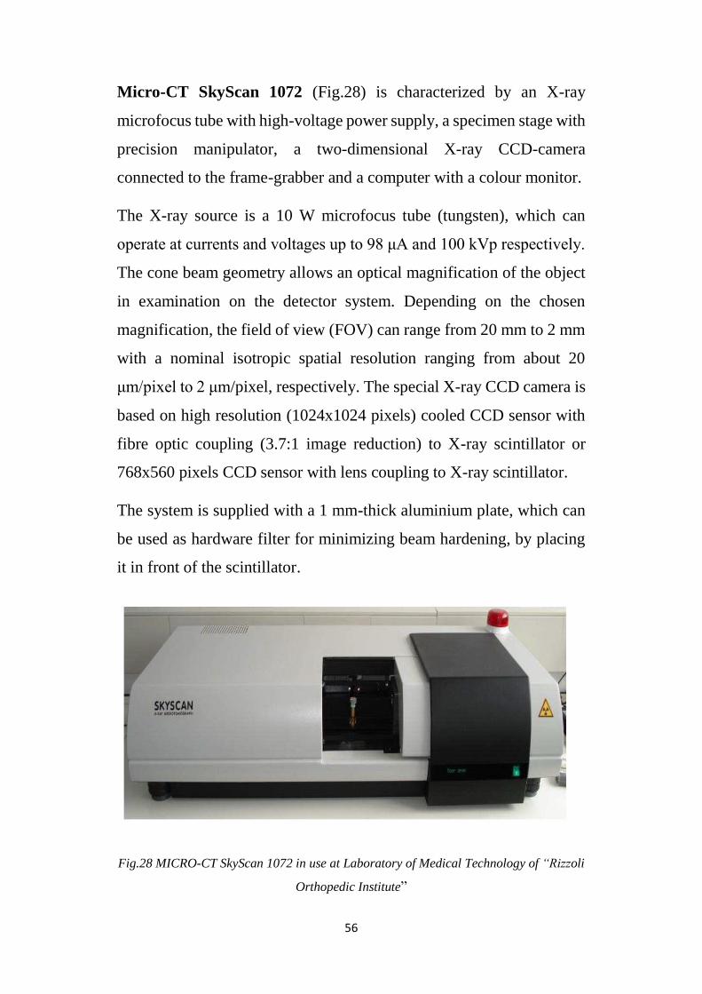
56

Micro-CT SkyScan 1072 (Fig.28) is characterized by an X-ray

microfocus tube with high-voltage power supply, a specimen stage with

precision manipulator, a two-dimensional X-ray CCD-camera

connected to the frame-grabber and a computer with a colour monitor.

The X-ray source is a 10 W microfocus tube (tungsten), which can

operate at currents and voltages up to 98 μA and 100 kVp respectively.

The cone beam geometry allows an optical magnification of the object

in examination on the detector system. Depending on the chosen

magnification, the field of view (FOV) can range from 20 mm to 2 mm

with a nominal isotropic spatial resolution ranging from about 20

μm/pixel to 2 μm/pixel, respectively. The special X-ray CCD camera is

based on high resolution (1024x1024 pixels) cooled CCD sensor with

fibre optic coupling (3.7:1 image reduction) to X-ray scintillator or

768x560 pixels CCD sensor with lens coupling to X-ray scintillator.

The system is supplied with a 1 mm-thick aluminium plate, which can

be used as hardware filter for minimizing beam hardening, by placing

it in front of the scintillator.

Fig.28 MICRO-CT SkyScan 1072 in use at Laboratory of Medical Technology of “Rizzoli

Orthopedic Institute”

57

Micro-CT SkyScan 1176 (Fig.29) has instead an X-ray microfocus

tube that operates in the range 20-90kVp, with a maximum power of

25W. The special X-ray CCD-camera is based on 11 Megapixel

(4000x2672 pixels) cooled CCD-sensor with fibre optic coupling to the

X-ray scintillator. The scanning area is 68mm x 200mm or 35mm x

200mm. It is based on spiral scan to avoid ring artefacts and partial scan

connections and the time for a full scanning cycle is less than 1 minute

(1Kx1K slice format). The minimum pixel size is 9 μm and the low-

contrast spatial resolutions is equal to 15 μm (10% MTF). The “bed” on

which to place the samples or the animals is available in carbon fiber or

polystyrene foam and it is integrated with a physiological monitoring

subsystem that provides breathing and heart-beat gating for proven

thoracic image improvement by synchronized acquisition

(“www.bruker.com,” n.d.).

Fig.29 – Micro-CT SkyScan 1176 in use at the “Rizzoli Orthopedic Institute”

58

As regards the Cone Beam CT diagnostic technique, scans were

performed with the use of a device produced by the manufacturer QR

SRL (hereinafter QR) based in via Silvestrini, 20, Verona (Italy). The

CBCT device is precisely the Cone Beam CT 3D NewTom 5G

(Fig.30), which, with spacious gantry and motorized bed, is capable of

scanning various anatomical areas of the body (“www.newtom.it,”

n.d.). The main features of the machine are the following: X-ray source,

with rotating anode, maximum voltage 110 kVp; 1-20 mA (pulsed

mode), focal spot of 0.3mm, scan time in the range 18-36s; it takes an

image at every degree of rotation that is of 360°. The image detector is

an amorphous silicon flat panel, with a 20 cm x 25 cm Field of View.

Cone Beam 3D imaging uses a cone-shaped beam to acquire the entire

image of the object in a single scan using only one rotation. It is mostly

applied for dental and maxillofacial investigations.

Fig. 30 – CBCT 3D NewTom 5G machine. Ref. www.newtom.it

59

4.3.3 Image Acquisition

For each sample abovementioned, scanning and subsequent comparison

was performed using different devices. The samples of group 1 were

scanned by micro-CT method using the device SkyScan 1176. Cone

Beam CT acquisition were done by using two different Newton 5G

devices. The first one was located at the “Spedali Civili” in Brescia in

collaboration with the “Medical Physics Unit”; the second one was

located at the “QR” of Verona, in collaboration with the “Imaging

Department”. The source of micro-CT SkyScan 1176 has been set at 80

kVp, 313 μA, using the 1 mm-Al filter for beam hardening

minimization. The exposure was fixed at 66 μs, the rotation step at

0.300 deg, smoothing at 1, ring artifact correction at 7 and image pixel

size at 34.95 μm.

The parameters set for the CBCT scans have been set at 110KVp with

an exposure time of 15s and image pixel size at 100 μm.Figures 31a and

31b show a frontal X-ray projection of one of the cylindrical cancellous

bone biopsies of femoral bone of a cadaver, obtained with SkyScan

1176 (a) and Cone Beam CT Newtom 5G (b) respectively.

Fig 31- Frontal X-ray projection obtained by means of micro-CT SkyScan 1176(a) and

CBCT Newton 5G(b) of a cylindrical bone biopsy with a image pixel size of 34,95 μm and

100 μm respectivily. Ref. Laboratory of Medical Technology at “Rizzoli Orthopedic

Institute”.

60

The specimens of group 2 were scanned by micro-CT method using the

SkyScan 1176 device and by Cone Beam CT using the Newton 5G

machine in use at the “Spedali Civili” in Brescia with the same

acquisition parameters of “sample type 1”. In this case, the datasets

obtained from the scans were subjected in advance to an operation

called “3D Registration” by means of the Software DataViewer

(Bruker, Belgium) so that the dataset selected as “target” is transformed

into the coordinate system of the dataset selected as “reference” which

stays stationary. More information about the Image Registration can be

found below.

The samples of group 3 were scanned with SkyScan 1176 and with

Newtom 5G in use at QR of Verona. Also in this case, the acquisition

parameters are the same used for the previous groups of samples. The

only difference in the scanning of the objects is that, while the samples

of groups 1 and 2 were scanned embedded in PMMA, the third type of

samples was scanned in air, wrapped in a layer of parafilm, an efficient

laboratory material, that with its high elasticity, guarantees optimal fit

and protects against evaporation, contamination and hydration. The

specimens were placed on the machine’s bed with their main transverse

axis parallel to that of the bed itself (in order to avoid reaching the limits

of the field of view where it has the more evident artifacts with

increasing resolution). Also in this case, the datasets scanned with two

different techniques, are “registered” to ensure that the images have the

same three-dimensional reference system.

4.3.4 Image Reconstruction

The reconstruction operation allows tracing information on the intensity

of beams attenuated in all directions and on the linear attenuation

61

coefficient relative to each volume element. The reconstruction of the

microtomographic images was performed by means of a special

software, provided by the home manufacturer of the device, the

SkyScan NRecon (Bruker, Belgium), in which the process is based on

a particular type of Feldkamp algorithm. The Feldkamp algorithm is the

most used for the reconstruction of images obtained with cone beam

tomography; it is based on the Radon transform, the mathematical tool

which ensures the reconstruction of an object from its projections. The

obtained images can be saved in different file formats; in this case, the

8-bit BMP format was chosen.

The output images from Cone Beam CT are DICOM images, a standard

and public format, now used in the vast majority of biomedical products

especially in the field of radiology.

4.3.5 Image Registration

For the samples of groups 2 and 3, it was necessary to apply the Image

Registration, in order to convert different sets of data into one

coordinate system. It is a recurring problem in the medical imaging, as

it is not possible to have a precise standardization of the scanning

process when the same subject is scanned in different times or even with

different tomographic methods. In this case, two different approaches

depending on the considered sample are used. In fact, for sample of

group 2 it was enough to use the software DataViewer (Bruker) to

record the various data sets of images (Fig.32).

62

Fig.32- An example of “3D Registration” function using DataViewer software. The

dataset selected as “target” is transformed into the coordinate system of the dataset

selected as “reference”

Once a reference and a target datasets have been set, the target is

transformed into the coordinate system of the reference that stays

stationary.

For sample of group 3, instead, the registration process was much more

laborious. DataViewer becomes efficient only for “small

displacements” and only if the datasets have been scanned in the same

way in the three axes of reference x, y, z. Conversely, the vertebrae

location varied from time to time in the two methods of scanning; for

this reason, the procedure was divided into several steps:

- converting images from BMP format to VTK format so that it could

be created, using the 3D graphics program ITK – SNAP, an STL file

that describes a raw unstructured triangulated surface by the unit

normal and vertices (ordered by the right-hand rule) of the triangles

using a three-dimensional Cartesian coordinate system. STL

63

coordinates must be positive numbers, there is no scale information,

and the units are arbitrary (Fig.33). Starting from it and from all the

slices related to the volume of interest of the sample (for each one),

it was reconstructed the three-dimensional image of the vertebra

(Fig. 34)

- manual roto-translation operations of the obtained 3D surfaces

through BUILDER software (free available at www.bonemat.com)

to obtain the corresponding matrix of rotational translation

- ad hoc optimization of that matrix with the use of MatLab scripts

(Matlab, The Mathworks Inc, Natick, MA,USA), which provide the

registration of an STL surface 'moving' on a STL surface 'target'.

- calculation of the Euler angles that describe the orientation of a rigid

body and in particular, the orientation of a coordinate system relative

to another.

- registration of a dataset in the other reference system in which

micro-CT dataset was defined as target and CBCT dataset as

moving.

Fig.33 – STL surface of a vertebra

64

Fig. 34 – Three-dimensional image of the vertebra reconstructed from STL surface

4.3.6 Validation of an optimal threshold for image

segmentation

Before proceeding with calculation of the histomorphometric

parameters, the grey level image has to be previously segmented into a

bone and non-bone phase. This process, also called “segmentation”,

“thresholding” or “binarization”, has as a result an image composed

only of black or white pixel, where black means non-bone while white

means bone.

First of all, it was appropriate to define a threshold value for the micro-

CT SkyScan 1176; in the absence of comparisons with the "real"

histological value of the samples, it was proceeded with the validation

of an “optimal thresholding” using the cross comparison with the

acquisitions on SkyScan 1072 of 5 samples of trabecular bone included

in PMMA at disposal, with BV/TV values between 6 and 25 % (the

same specimens previously identified as sample type 1). The scans of

these samples on the SkyScan 1176, conducted with the same

65

acquisition parameters, were analyzed with variable thresholds (about

100 thresholds for each specimen) up to replicate the BV/TV values

acquired on SkyScan 1072 with the trabecular bone protocol. The used

method was the Minimum Variation of the parameter in question: for

example, for BV/TV parameter, the change in bone volume fraction

(BV/TV) in relation to the threshold value was investigated; then, the

value corresponding to the minimum variation of BV/TV parameter

variation, was selected as the global threshold value (Ding, Odgaard, &

Hvid, 1999).

The same mechanism was used to identify the optimal “threshold” for

the elaboration of the tomographic images from Cone Beam CT

Newtom 5G taking, as a reference, the threshold value previously

obtained from micro-CT SkyScan 1176.

For the sample of the group 2, the validation of an optimal threshold

has been performed in a different way because the protocol used above,

is applicable mostly in samples characterized by trabecular tissue. For

cortical tissue, instead, a technique has been used where a single

threshold value is selected, based on the distribution of the gray levels

in the images. The histogram of these images, in fact has two rather

obvious peaks, corresponding to the bone material (lowest peak) and

the background (highest peak); the optimal threshold is therefore

identified in the minimum point between the two peaks.

4.3.7 Image Segmentation and Calculation of the

Histomorphometric Parameters

Through the software released by the Bruker manufacturer (SkyScan,

Belgium), Ct–Analyser, first the identification of a Region of Interest

(ROI) was done in order to perform 3D calculations. Specifically, for

66

the sample of the group 1, a circle ROI of 9 mm was defined,

interpolating it over the whole dataset taken into account. For the

sample types 2 and 3, a manually defined polygonal ROI was chosen,

in order to select the trabecular tissue. In the first case, accurate

attention has been paid to identify only cortical tissue; conversely, in

the second case the vertebrae have been "cleaned" ad hoc from cortical

bone tissue to select only trabecular tissue. Subsequently, with the

defined threshold, the image binarization was carried out. The pictures

below show an example of cross-sectional image for each group of

samples and the corresponding segmented images, obtained with

micro-CT (Fig.35) and Cone Beam CT (Fig.36) scanners, respectively.

With global threshold, the histomorphometric parameters discussed

above were estimated over a selected volume of interest (VOI) of

micro-CT slices for each specimen. The volume of interest is chosen

taking the greatest possible number of slices. For trabecular bone, the

attention was focused on the BV/TV (%), Tb.Th (mm) and Tb.Sp (mm).

For the cortical bone analysis, instead, the calculations involved DA

and Total Porosity (%).

67

Fig. 35 - Cross-sections and corresponding segmented images obtained with

micro-CT scanner SkyScan 1176 and Ct-Analyser Software. Ref. Laboratory of

Medical Technology at the “Rizzoli Orthopedic Institute”

68

Fig. 36 - Cross-section and corresponding segmented images obtained with

scanner Cone Beam CT 5G and Ct-Analyser Software. Ref. Laboratory of

Medical Technology at the “Rizzoli Orthopedic Institute”

4.4 Statistical Analysis

The correlation between different methods was analyzed by using the

Linear Regression Model.

Linear regression is the most basic and commonly used predictive

analysis. Regression estimates are used to describe data and to explain

the relationship between one dependent variable and one or more

independent variables. At the core of the regression analysis is the task

69

of fitting a single line through a scatter plot. The simplest form with

one dependent and one independent variable is defined by the formula

y = c + b*x

where y is the estimated dependent variable, c is a constant, b is the

regression coefficient and x is the independent variable. Linear

regression analysis consists of more than just fitting a linear line

through a cloud of data points, it consists of 3 particular stages:

analyzing the correlation and directionality of the data, estimating the

model, i.e., fitting the line, and evaluating the validity and usefulness of

the model. Adding independent variables to a linear regression model

will always increase the explained variance of the model (typically

expressed as R²).

R2, the coefficient of determination, is a number that indicates the

proportion of the variance in the dependent variable that is predictable

from the independent variable, it gives some information about the

goodness of fit of a model because it is a measure of how well the

regression line approximates the real data points. An R2 of 1 indicates

that the regression line perfectly fits the data, while values of R2 close

to zero may occur when fitting non-linear functions to data.

70

CHAPTER 5

Analysis of Results

In this chapter, the results of all measurements taken on the three

different groups of samples are described and analyzed.

5.1 Defining the optimal threshold value for SkyScan 1176

micro-CT scanner

As mentioned in the Chapter 4, before proceeding to the segmentation

of the images and to the relative calculation of the structural parameters,

it was appropriate to define a threshold value for elaboration of the

images obtained by means of the SkyScan 1176 micro-CT scanner. For

this purpose, in the absence of comparison with the parameters

calculated histologically, the method of Minimum Variation was used

as previously explained. The comparison was based on the knowledge

of the optimal threshold for the segmentation of images obtained with

SkyScan 1072, calculated in a previous study carried out at the Medical

Technology Laboratory of Rizzoli Orthopedic Institute by using the

same specimens of group 1. The threshold calculated for SkyScan 1072

is equal to 117 in a scale of 256 gray-levels. Through the calculation of

Minimum Variation, the threshold identified as “optimal” for the

segmentation of images obtained by the SkyScan 1176 amounted to

123.

The functional relationship between the variables was evaluated

through the simple Linear Regression Model calculating the coefficient

of determination to estimate the proportion between the variability of

the data and the correctness of the employed statistical model.

71

Table 2 below, contains the BV/TV (%) values calculated from the

microtomographic images obtained with SkyScan 1072 and SkyScan

1176 with both devices at different thresholds (117 and 123

respectively) and the corresponding Linear Regression Model (Fig. 37).

SAMPLE TYPE 1 BV/TV (%) SkyScan 1072 BV/TV (%) SkyScan 1176

Specimen 1 12,4±0,3 12,4±0,9

Specimen2 20,0±0,5 21,3±1,6

Specimen 3 7,14±0,17 6,5±0,5

Specimen4 16,8±0,4 18,1±1,3

Specimen 5 25,4±0,6 28,2±2,1

Tab. 2 – Values of BV/TV (%) calculated from the microtomographic images of the first

group of samples, obtained with SkyScan 1072 (threshold value equal to 117) SkyScan

1176 (threshold value equal to 123).

Fig.37 – Regression Linear Model for BV/TV (%) values obtained with SkyScan 1072

(threshold 117) and those obtained with SkyScan 1176 (threshold 123).

R2 gives some information about the fit of each model. In this case, the

coefficient of determination R2 is a statistical measure of how well the

y = 1,1853x - 2,0144R² = 0,9989

0

5

10

15

20

25

30

0 5 10 15 20 25 30

BV

/TV

(%

) m

-CT

11

76

BV/TV (%) m-CT1072

Regression Linear Model - SkyScan 1072 vs SkyScan 1176

72

regression line approximates the real data points. The results of R2=

0,9989 indicates that the regression line almost perfectly fits the data.

For this reason, all the calculations in the segmentation of images

obtained with the SkyScan 1176 scanners will be carried out using 123

as threshold value.

5.2 Analysis of measurements performed on SAMPLE type 1

Sample type 1 is characterized by 5 cylindrical biopsies from femoral

bone of cadavers with only trabecular tissue embedded in PMMA. The

scans were performed with SkyScan 1176 and both Cone Beam Newton

5G devices (installed in Brescia and Verona). For this reason, the

parameter BV/TV (%), Tb.Th (mm) and Tb.Sp (mm), which are good

descriptors of the trabecular structure, were calculated.

The method of the Minimum Variation was used again to calculate the

optimal threshold value to process the images scanned with the

NewTom 5G Cone Beam CT. The obtained results have quantified 157

as threshold value for the device installed at "Spedali Civili" of Brescia,

while a value of 100 for the scanner installed at Verona QR. Since for

Sample type 1 scans performed with micro-CT SkyScan 1072 were

available, the calculation of each parameter was also performed on

these data for the comparison with the two Cone Beam CT devices.

In the following graphs the values of the bone parameters calculated

from the cone beam CT images are reported on the y-axis, while the

corresponding values, obtained from micro-CT, are on x-axis. For each

graph the equation of the linear regression and the corresponding

coefficient of determination are reported.

73

Tab- 3 BV/TV (%) values calculated on the images obtained with different scanners using

the previously defined thresholds for segmentation.

Fig 38 – BV/TV values obtained by means of micro-CT (SkyScan 1072 and SkyScan

1176) and Cone Beam CT NewTom 5G in Brescia.

Fig 39 - BV/TV values obtained by means of micro-CT (SkyScan 1072 and SkyScan 1176)

and Cone Beam CT NewTom 5G in Verona.

y = 1,4022x - 5,5665R² = 0,7852

y = 1,6832x - 8,8021R² = 0,8068

0

5

10

15

20

25

30

35

40

45

50

0 5 10 15 20 25 30

BV

/TV

(%

) C

BC

T (B

RES

CIA

)

BV/TV (%) micro-CT

Comparison BV/TV (%) between micro-CT and Cone Beam CT(Brescia)

SkyScan 1176

SkyScan 1072

y = 2,1732x - 16,17R² = 0,9639

y = 2,5778x - 20,681R² = 0,9673

0

5

10

15

20

25

30

35

40

45

50

0 5 10 15 20 25 30

BV

/TV

(%

) C

BC

T (V

ERO

NA

)

BV/TV (%) micro-CT

Comparison BV/TV (%) between micro-CT and Cone Beam CT(Verona)

SkyScan 1176

SkyScan 1072

SAMPLE type 1 BV/TV (%)

SkyScan 1072 BV/TV (%)

SkyScan 1176

BV/TV (%) NewTom 5G

(Brescia)

BV/TV (%) NewTom 5G

(Verona)

Specimen 1 12,4 ± 0,3 12,4 ± 0,9 7,2 ± 0,4 7,4 ± 0,4

Specimen2 20,1 ± 0,5 21,3 ± 1,6 32,9 ± 1,6 33,3 ± 1,6

Specimen 3 7,14 ± 0,17 6,5 ± 0,5 4,4 ± 0,2 1,21 ± 0,06

Specimen4 16,8 ± 0,4 18,1 ± 1,3 14,6 ± 0,7 19,3 ± 0,9

Specimen 5 25,4 ± 0,6 28 ± 2 28,9 ± 1,4 46 ± 2

74

Tab 4 – Tb.Th (mm) values calculated on the images obtained with different scanners

using the previously defined thresholds for segmentation.

Fig 40 – Tb.Th (mm) values obtained by means of micro-CT (SkyScan 1072 and SkyScan

1176) and Cone Beam CT NewTom 5G in Brescia.

Fig 41 – Tb.Th (mm) values obtained by means of micro-CT (SkyScan 1072 and SkyScan

1176) and Cone Beam CT NewTom 5G in Verona.

y = 2,0325x + 0,0677R² = 0,9265

y = 2,5592x + 0,0109R² = 0,902

0

0,1

0,2

0,3

0,4

0,5

0,6

0,7

0,12 0,14 0,16 0,18 0,2 0,22 0,24 0,26

Tb.T

h (

mm

) C

BC

T (B

RES

CIA

)

Tb.Th (mm) micro-CT

Comparison Tb.Th (mm) between micro-CT and Cone Beam CT(Brescia)

SkyScan 1176

SkyScan 1072

y = 2,8489x - 0,1155R² = 0,9459

y = 3,556x - 0,1897R² = 0,9049

0

0,1

0,2

0,3

0,4

0,5

0,6

0,7

0,12 0,14 0,16 0,18 0,2 0,22 0,24 0,26

Tb.T

h (

mm

) C

BC

T (V

ERO

NA

)

Tb.Th (mm) micro-CT

Comparison Tb.Th (mm) between micro-CT and Cone Beam CT(Verona)

SkyScan 1176

SkyScan 1072

SAMPLE type 1 Tb.Th (mm)

SkyScan 1072 Tb.Th (mm)

SkyScan 1176

Tb.Th (mm) NewTom 5G

(Brescia)

Tb.Th (mm) NewTom 5G

(Verona)

Specimen 1 0,1559 ± 0,0012 0,166 ± 0,004 0,365 ± 0,018 0,331 ± 0,016

Specimen2 0,1916 ± 0,0015 0,208 ± 0,005 0,49 ± 0,02 0,44 ± 0,02

Specimen 3 0,1391 ± 0,0011 0,145 ± 0,004 0,375 ± 0,018 0,307 ± 0,015

Specimen4 0,1492 ± 0,0012 0,163 ± 0,004 0,42 ± 0,02 0,384 ± 0,019

Specimen 5 0,2195 ± 0,0017 0,251 ± 0,006 0,58 ± 0,03 0,62 ± 0,03

75

Tab 5 – Tb.Sp (mm) values calculated on the images obtained with different scanners

using the previously defined thresholds for segmentation.

Fig 42 – Tb.Sp (mm) values obtained by means of micro-CT (SkyScan 1072 and SkyScan

1176) and Cone Beam CT NewTom 5G in Brescia.

Fig 43 – Tb.Sp (mm) values obtained by means of micro-CT (SkyScan 1072 and SkyScan

1176) and Cone Beam CT NewTom 5G in Verona.

y = 1,9831x - 0,1784R² = 0,6758

y = 2,1489x - 0,2706R² = 0,6409

0

0,5

1

1,5

2

2,5

0,4 0,5 0,6 0,7 0,8 0,9 1 1,1 1,2

Tb.S

p (

mm

) C

BC

T (B

RES

CIA

)

Tb.Sp (mm) micro-CT

Comparison Tb.Sp (mm) between micro-CT and Cone Beam CT(Brescia)

SkyScan 1176

SkyScan 1072

y = 3,9845x - 1,8185R² = 0,8312

y = 4,3617x - 2,0394R² = 0,8045

0

0,5

1

1,5

2

2,5

3

3,5

0,4 0,5 0,6 0,7 0,8 0,9 1 1,1 1,2

Tb.S

p (

mm

) C

BC

T (V

ERO

NA

)

Tb.Sp (mm) micro-CT

Comparison Tb.Sp (mm) between micro-CT and Cone Beam CT(Verona)

SkyScan 1176

SkyScan 1072

SAMPLE type 1 Tb.Sp (mm)

SkyScan 1072 Tb.Sp (mm)

SkyScan 1176

Tb.Sp (mm) NewTom 5G

(Brescia)

Tb.Sp (mm) NewTom 5G

(Verona)

Specimen 1 0,921 ± 0,014 0,94 ± 0,02 1,62 ± 0,08 1,59 ± 0,08

Specimen2 0,76 ± 0,012 0,77 ± 0,02 0,95 ± 0,04 0,86 ± 0,04

Specimen 3 1,074 ± 0,017 1,12 ± 0,03 2,20 ± 0,11 3,01 ± 0,15

Specimen4 0,647 ± 0,011 0,66 ± 0,01 1,49 ± 0,07 1,19 ± 0,06

Specimen 5 0,643 ± 0,011 0,63 ± 0,01 1,07 ± 0,05 0,80 ± 0,04

76

As the graphs show, the obtained results are more than satisfactory. In

most cases (except in the evaluation of Tb.Sp compared with NewTom

5G of Brescia, p<0.05), the coefficients of determination R2 range from

0,8 to 0,96 (p<0.008). Therefore, not only a positive correlation of data

is present but also a very strong association of variables.

However, it is worth noting that the two Cone Beam CT presented a

different behavior. Although both devices are the same model, it has to

be mentioned that the NewTom 5G installed at “Spedali Civili”-

Brescia has a very intense clinical load, while the NewTom 5G installed

at QR-Verona is mostly dedicated to research and development and

reasonably it does not have the same amount of use. In any case, it can

be said that the outcome of the test satisfies the initial premises.

5.3 Analysis of measurements performed on SAMPLE type 2

For Sample type 2, which includes 3 biopsies of tibial bone from

cadavers characterized by only cortical tissue, a technique based on the

distribution of the gray levels present on images was used to

determinate the threshold value. It is a purely subjective operation since

it is based on the “good eye” operator and his experience. To segment

the images scanned with micro-CT SkyScan 1176, a threshold value of

148 (for cortical bone) was chosen, while the correspondent threshold

value for CBCT NewTom 5G (Brescia) was found at 175. The Tables

below show the values of the Degree of Anisotropy and Total Porosity

estimated by Ct-Analyser software (Bruker) with the thresholds

mentioned above, while in the graphs the corresponding Linear

Regression Model is reported.

77

SAMPLE type 2 DA SkyScan 1176 DA NewTom 5G (Brescia)

Specimen 1 1,94 ± 0,15 2,81 ± 0,14

Specimen2 2,05 ± 0,16 3,10 ± 0,15

Specimen 3 2,24 ± 0,18 4,4 ± 0,2

Tab 6 – Degree of Anisotropy values calculated from images obtained with micro-CT

SkyScan 1176 and Cone Beam CT NewTom 5G in Brescia.

Fig. 44 – Comparison of the Degree of Anisotropy values calculated on images obtained

with Micro-CT SkyScan 1176 and Cone Beam CT NewTom 5G in Brescia.

SAMPLE type 2 Po(tot)(%) SkyScan

1176 Po(tot)(%) NewTom 5G

(Brescia)

Specimen 1 2,24 ± 0,07 0,66 ± 0,03

Specimen2 1,96 ± 0,06 0,71 ± 0,03

Specimen 3 1,49 ± 0,05 0,40 ± 0,02

Tab 7 – Total Porosity values (%) calculated from images obtained with micro-CT

SkyScan 1176 and Cone Beam CT NewTom 5G in Brescia.

y = 5,4561x - 7,8952R² = 0,9625

0,00000

0,50000

1,00000

1,50000

2,00000

2,50000

3,00000

3,50000

4,00000

4,50000

5,00000

1,90000 1,95000 2,00000 2,05000 2,10000 2,15000 2,20000 2,25000 2,30000

DA

cb

ct N

ewTo

m 5

G (

BR

ESC

IA)

DA micro-CT SkyScan 1176

Comparison Degree of Anistotropy between SkyScan 1176 and CBCT (Brescia)

78

Fig. 45 – Comparison of the Total Porosity (%) values calculated on images obtained

with Micro-CT SkyScan 1176 and Cone Beam CT NewTom 5G in Brescia.

Also for the samples of group 2, through the Linear Regression graph,

a good correlation between the data is found, with coefficient of

determination R2 equal to respectively 0,96 (p<0.1) and 0,74 (p<0.3).

5.4 Analysis of measurements performed on SAMPLE type 3

The comparison for Sample type 3 was done on images scanned with

micro-Ct SkyScan 1176 and Cone Beam CT NewTom 5G installed at

QR in Verona. Seventeen thoracic and lumbar vertebrae of cadavers

with both trabecular and cortical bone were analyzed. Vertebrae

belonged to severely osteoporotic donor subjects. With a polygonal ROI

interpolated throughout the dataset, the BV/TV (%) was calculated by

means of Ct-Analyser software (Bruker). Subsequently a comparison of

the two methods of imaging discussed until now was performed.

The optimal threshold adopted for the image segmentation is 97 and it

is equal to the arithmetic mean of the thresholds calculated for each

sample with the method of Minimum Variation. In this case the

y = 0,3715x - 0,112R² = 0,748

0,00000

0,10000

0,20000

0,30000

0,40000

0,50000

0,60000

0,70000

0,80000

0,50000 1,00000 1,50000 2,00000 2,50000

Po

(to

t) (

%)

cbct

New

Tom

5G

(B

RES

CIA

)

Po (tot) (%) micro-CT SkyScan 1176

Comparison Total Porosity between SkyScan 1176 and CBCT (Brescia)

79

variability of the thresholds was very high (from 48 to 133), but the aim

was to find a global threshold valid for all the samples.

Tab 8 – BV/TV (%) values calculated from the images obtained with SkyScan

1176 and NewTom 5G in Verona.

* it is not a real value; Software is unable to calculate it.

From the table 8 it can be seen a certain discrepancy between the

obtained values. The same discrepancy is even more clear in Fig. 46,

in which the coefficient of determination R2 = 0,03 shows a total lack

of correlation between the data.

SAMPLE type 3 BV/TV (%) SkyScan 1176 BV/TV (%) NewTom 5G

(Verona)

Specimen 1 13,51 ± 1,02 59±3

Specimen2 12,8 ± 0,9 17,5 ± 0,8

Specimen 3 3,2 ± 0,2 0,018 ± 0,001

Specimen 4 3,0 ± 0,2 0∗

Specimen 5 3,6 ± 0,2 0,012 ± 0,001

Specimen 6 4,3 ± 0,3 27,3 ± 1,3

Specimen 7 25,1 ± 1,6 3,43 ± 0,17

Specimen 8 12,5 ± 0,9 17,1 ± 0,8

Specimen 9 8,1 ± 0,6 0,94 ± 0,04

Specimen 10 3,6 ± 0,2 0,014 ± 0,001

Specimen 11 5,9 ± 0,5 0,018 ± 0,001

Specimen 12 5,7 ± 0,4 22,59 ± 1,13

Specimen 13 5,6 ± 0,4 38,0 ± 1,9

Specimen 14 7,6 ± 0,6 2,87 ± 0,14

Specimen 15 6,8 ± 0,5 1,41 ± 0,07

Specimen 16 7,9 ± 0,6 19,2 ± 0,9

Specimen 17 8,2 ± 0,6 0,45 ± 0,02

80

Fig. 46– Comparison of BV/TV (%) values calculated on the images obtained with micro-

CT SkyScan 1176 and Cone Beam CT NewTom 5G in Verona.

To improve the obtained results, a Sharpening filter (implemented in

Ct-Analyser Software) was applied to images scanned with Cone Beam

CT. The obtained values slightly improve but the low coefficient of

determination obtained from Linear Regression Model (Fig. 47)

confirms the total non-correlation between the data.

y = 0,5664x + 7,7629R² = 0,0338

0,00000

10,00000

20,00000

30,00000

40,00000

50,00000

60,00000

70,00000

0 5 10 15 20 25 30

BV

/TV

(%

) N

ewTo

m 5

G (

VER

ON

A)

BV/TV (%) SkyScan 1176

Comparison BV/TV (%) between micro-CT and Cone Beam CT(Verona)

81

Tab 8 – BV/TV (%) values calculated from the images obtained with SkyScan 1176 and

NewTom 5G in Verona, after the application of a Sharpening Filter

Fig. 47 – Comparison of BV/TV (%) values calculated on the images obtained with

micro-CT SkyScan 1176 and Cone Beam CT NewTom 5G in Verona, after the application

of a Sharpening Filter.

y = 0,9048x + 7,1522R² = 0,0972

0,00000

10,00000

20,00000

30,00000

40,00000

50,00000

60,00000

0 5 10 15 20 25 30BV

/TV

(%

) N

ewTo

m 5

G (

VER

ON

A)

BV/TV (%) SkyScan 1176

Comparison BV/TV (%) between micro-CT and Cone Beam CT(Verona)with SHARPENING FILTER

SAMPLE type 3 BV/TV (%) SkyScan

1176

BV/TV (%) NewTom 5G (Brescia)

SHARPENING FILTER

Specimen 1 13,51 ± 1,02 55,1 ± 2,7

Specimen2 12,8 ± 0,9 28,2 ± 1,4

Specimen 3 3,2 ± 0,2 2,38 ± 0,12

Specimen 4 3,0 ± 0,2 0,067 ± 0,003

Specimen 5 3,6 ± 0,2 0,014 ± 0,007

Specimen 6 4,3 ± 0,3 32,29252

Specimen 7 25,1 ± 1,6 10,9 ± 1,6

Specimen 8 12,5 ± 0,9 22,65 ± 1,13

Specimen 9 8,1 ± 0,6 4,2 ± 0,2

Specimen 10 3,6 ± 0,2 0,167 ± 0,008

Specimen 11 5,9 ± 0,5 0,094 ± 0,004

Specimen 12 5,7 ± 0,4 18,5 ± 0,9

Specimen 13 5,6 ± 0,4 33,6 ± 1,6

Specimen 14 7,6 ± 0,6 8,2 ± 0,4

Specimen 15 6,8 ± 0,5 5,4 ± 0,2

Specimen 16 7,9 ± 0,6 22,75 ± 1,13

Specimen 17 8,2 ± 0,6 1,75 ± 0,08

82

CHAPTER 6

Discussion of Results

6.1 Considerations about the measurements

performed on the 3 types of Sample

In the Chapter 5, the results, obtained after the laborious measurements

on the three available types of samples, have been shown.

The purpose of this thesis is to compare the morpho-structural

parameters that characterize the bone tissue and in particular the

trabecular tissue, calculated on images obtained through two methods

of tomographic imaging.

For the first two types of samples (5 biopsies of femoral bone and 3

biopsies of tibial bone), as documented also with the graphs in

paragraphs 5.2 and 5.3, the obtained results show a significant

correlation between the two sets of data using a global threshold value

for the segmentation of the images. This demonstrate, therefore, a

positive outcome for the comparison of the two methods of

tomographic imaging used for all the tests and it gives a positive answer

to the main question of this thesis. It is, however, worth pointing out

that the Samples type 1 and 2 correspond to extremely ideal cases: bone

tissue, completely trabecular or completely cortical, of small

dimensions, embedded in PMMA that has a coefficient of attenuation

similar to that of water.

As regards the Sample type 3, instead, the same positive answer was

not found. Indeed, the negative results certainly exclude the use of a

global threshold for image processing. However, it is good to pay close

83

attention to the conditions in which the samples were scanned: we are

in a real case that is not remotely close to the optimal conditions of the

other (small specimens embedded in biocompatible material).

Several could be the causes that can be attributed to these results: for

example, the scan mode (which was done in air), the quality of the

beam, the use of a little appropriate software for the processing of the

images (Ct- Analyser was created above all for the processing of micro-

CT images), and, not least, the pathological severity of the disease from

which the donors were suffering. In fact it is easy to see that many

samples analyzed had a really to low BV/TV (about 3 %).

A possible explanation for the poor results obtained for the Sample type

3 can also be attributed to the use, for the calculation of structural

parameters, of a software that necessarily requires the binarization of

the images’ dataset in only white or black pixels. In this case, it becomes

very difficult, even to the naked eye, to distinguish what is bone, what

is marrow or water when lower spatial resolutions than those obtained

by micro-tomography (defined as “gold standard”) are involved.

In fact, micro-CT is a powerful and consolidated tool for the three-

dimensional investigation of bone samples, allowing a quantitative

characterization of the microarchitecture at high resolution and in a

non-destructive way.

The use of bone tissue descriptors, already present in literature, which

avoid the segmentation of the images, could be very efficient in

evaluating the comparison between micro-CT and Cone Beam CT.

84

6.2 Future Developments

The research will proceed with the analysis of descriptors of the bone

quality based on structural tensors, such as the fabric tensor or the

gradient structure tensor.

A preliminary attempt has already been made through the use of the

Gradient Structure Tensor (GST). Structure tensors are a matrix

representation of partial derivative information. In the field of image

processing and computer vision, it is typically used to represent the

gradient or "edge" information. The term "tensor" refers to a

representation of an array of data where L1, L2, L3 and e1, e2, e3 are

the eigenvalues and eigenvectors respectively. These components can

be visualized as 3D ellipses where the radii are equal to the eigenvalues

in descending order and directed along their corresponding

eigenvectors. Using gradient-based structure tensors, local patterns of

contours and surfaces may be inferred through a diffusion process

(Nicolescu & Medioni, 2003). Many studies demonstrated, for

example, that the method to determine trabecular main direction in situ

is GST. (Wolfram, Schmitz, Heuer, Reinehr, & Wilke, 2009). Knowing

the main direction, a transverse isotropic fabric tensor can be

constructed.

In the attempt abovementioned, a Matlab implementation available

online was used (Arseneau, 2006); it has produced partial results,

applicable, however, only in the 2D case. An ad hoc implementation

could give more satisfactory results applicable in 3D, in order to

confirm the positive answer found in Sample type 1 and 2 also in real

cases that undoubtedly have poor conditions, much more difficult to

manage.

85

86

REFERENCES

Adams, J. E. (2009). Quantitative computed tomography. European Journal of

Radiology, 71(3), 415–424. http://doi.org/10.1016/j.ejrad.2009.04.074

Anderson, H. C. (2003). Matrix vesicles and calcification. Current Rheumatology

Reports, 5(3), 222–226. http://doi.org/10.1007/s11926-003-0071-z

Arseneau, S. (2006). http://www.mathworks.com.

Bone Density Scan. (n.d.). Retrieved from http://www.rwrad.com/Bone-Density.html

Buckwalter, J. A., Glimcher, M. J., Cooper, R. R., & Recker, R. (1996). Bone

biology. I: Structure, blood supply, cells, matrix, and mineralization.

Instructional Course Lectures, 45, 371–86. http://doi.org/10.3390/jfb1010022

Celenk, C., & Celenk, P. (2008). Bone Density Measurement Using Computed

Tomography. In Computed Tomograpy - Clinical Applications (pp. 123–136).

Clifford J. Rosen, Roger Bouillon, Juliet E. Compston, V. R. (2013). Primer on the

Metabolic Bone Diseases and Disorders of Mineral Metabolism. (Wiley-

Blackwell, Ed.).

Compston, J. (2006). Bone quality: what is it and how is it measured? Arquivos

Brasileiros de Endocrinologia E Metabologia, 50(4), 579–585.

http://doi.org/S0004-27302006000400003 [pii]

Cosman, F., de Beur, S. J., LeBoff, M. S., Lewiecki, E. M., Tanner, B., Randall, S., &

Lindsay, R. (2014). Clinician’s Guide to Prevention and Treatment of

Osteoporosis. Osteoporosis International, 25(10), 2359–2381.

http://doi.org/10.1007/s00198-014-2794-2

Cowin, S., & Telega, J. (2003). Bone Mechanics Handbook, 2nd Edition. -. In

Applied Mechanics Reviews (Vol. 56, p. B61). http://doi.org/10.1115/1.1579463

Dendy, P. P., Heaton, B., & Cameron, J. (2001). Physics for Diagnostic Radiology.

Medical Physics. http://doi.org/10.1118/1.1350686

Ding, M., Odgaard, A., & Hvid, I. (1999). Accuracy of cancellous bone volume

fraction measured by micro-CT scanning. Journal of Biomechanics, 32(3), 323–

326. http://doi.org/10.1016/S0021-9290(98)00176-6

Elliott, J. C., & Dover, S. D. (1982). X-ray Microtomography. Journal of

Microscopy, 126(2), 211–213. http://doi.org/10.1111/j.1365-

2818.1982.tb00376.x

Florencio-Silva, R., Rodrigues, G., Sasso, S., Sasso-Cerri, E., Simões, M. J., & Cerri,

87

P. S. (2015). Biology of Bone Tissue: Structure, Function, and Factors That

Influence Bone Cells. BioMed Research International, 1–17.

http://doi.org/10.1155/2015/421746

Franz-Odendaal, T. A., Hall, B. K., & Witten, P. E. (2006). Buried alive: How

osteoblasts become osteocytes. Developmental Dynamics.

http://doi.org/10.1002/dvdy.20603

Gilbert SF. Developmental Biology. (2000). Osteogenesis: The Development of

Bones. Development Biology: 6th Edition,

http://www.ncbi.nlm.nih.gov/books/NBK10056/. http://doi.org/10: 0-87893-243-

7

Goldman, L. W. (2007). Principles of CT and CT technology. Journal of Nuclear

Medicine Technology, 35(3), 115–28; quiz 129–30.

http://doi.org/10.2967/jnmt.107.042978

Goulet, R. W., Goldstein, S. A., Ciarelli, M. J., Kuhn, J. L., Brown, M. B., &

Feldkamp, L. A. (1994). The relationship between the structural and orthogonal

compressive properties of trabecular bone. Journal of Biomechanics, 27(4).

http://doi.org/10.1016/0021-9290(94)90014-0

Guglielmi, G. (2010). Assessment of Bone Quality and Structure. Clin Cases Miner

Bone Metab.

Guglielmi, G., Grimston, S. K., Fischer, K. C., & Pacifici, R. (1994). Osteoporosis:

diagnosis with lateral and posteroanterior dual x-ray absorptiometry compared

with quantitative CT. Radiology, 192(3), 845–850.

http://doi.org/10.1148/radiology.192.3.8058958

Hildebrand, T., & Rüegsegger, P. (1997). A new method for the model-independent

assessment of thickness in three-dimensional images. Journal of Microscopy,

185(1), 67–75. http://doi.org/10.1046/j.1365-2818.1997.1340694.x

Horton W A. (1990). The biology of bone growth. Growth Genet. Horm, (6(2):1–3).

Hubbell, J. H., & Seltzer, S. M. (1995). Tables of X-Ray mass attenuation coefficients

and mass energy-absorption coefficients 1 keV to 20 MeV for Elements Z=1 to 92

and 48 Additional substances of Dosimetric Interest.

http://physics.nist.gov/xaamdi. Retrieved from

http://www.nist.gov/pml/data/xraycoef/index.cfm

Issever, A. S., Link, T. M., Kentenich, M., Rogalla, P., Burghardt, A. J., Kazakia, G.

J., … Diederichs, G. (2010). Assessment of trabecular bone structure using

MDCT: Comparison of 64- and 320-slice CT using HR-pQCT as the reference

standard. European Radiology, 20(2), 458–468. http://doi.org/10.1007/s00330-

009-1571-7

J Van Dessel, Y Huang, M Depypere, I Rubira-Bullen, F. M. and R. J. (2013). A

88

comparative evaluation of cone beam CT and micro-CT on trabecular bone

structures in the human mandible. Dentomaxillofac Radiology.

Jerrold T. Bushberg, J. Anthony Seibert, Edwin M. Leidholdt Jr., J. M. B. (2002). The

Essential Physics of Medical Imaging (2nd Edition). (Lippincott Williams &

Wilkins, Ed.).

Kak, A. C., Author, Slaney, M., Wang, G., & Reviewer. (2002). Principles of

Computerized Tomographic Imaging. Medical Physics, 29, 107–107.

http://doi.org/10.1118/1.1455742

Keith Gibbs. (2006). Advanced Physics. (C. U. Press, Ed.).

Liu, Y., Saha, P. K., & Xu, Z. (2012). Quantitative characterization of trabecular

bone micro-architecture using tensor scale and multi-detector CT imaging.

Medical Image Computing and Computer-Assisted Intervention : MICCAI ...

International Conference on Medical Image Computing and Computer-Assisted Intervention, 15(Pt 1), 124–131.

Melton. (1992). No Title. Retrieved from

http://www.orthop.washington.edu/?q=patient-

care/articles/bone/osteoporosis.html

Naitoh, M., Aimiya, H., Hirukawa, A., & Ariji, E. (2010). Morphometric analysis of

mandibular trabecular bone using cone beam computed tomography: an in vitro

study. The International Journal of Oral & Maxillofacial Implants, 25(6), 1093–

8. Retrieved from http://www.ncbi.nlm.nih.gov/pubmed/21197484

Nicolescu, M., & Medioni, G. (2003). Motion segmentation with accurate boundaries

- a tensor voting approach. 2003 IEEE Computer Society Conference on

Computer Vision and Pattern Recognition, 2003. Proceedings., 1(June).

http://doi.org/10.1109/CVPR.2003.1211379

Noble, B. S. (2008). The osteocyte lineage. Archives of Biochemistry and Biophysics.

http://doi.org/10.1016/j.abb.2008.04.009

Odgaard, A. (1997). Three-dimensional methods for quantification of cancellous

bone architecture. Bone. http://doi.org/10.1016/S8756-3282(97)00007-0

Parfitt AM, Drezner MK, Glorieux FH, Kanis JA, Malluche H, Meunier PJ, Ott SM,

R. R. (1987). Bone Histomorphometry: standardization of nomenclature,

symbols and units. Journal of Bone and Mineral Research 2.

Parsa, A., Ibrahim, N., Hassan, B., van der Stelt, P., & Wismeijer, D. (2015). Bone

quality evaluation at dental implant site using multislice CT, micro-CT, and cone

beam CT. Clinical Oral Implants Research, 26(1), e1–e7.

http://doi.org/10.1111/clr.12315

Perilli. (2006). Microtomographic techniques for the characterization of bone tissue.

89

Poludniowski, G., Landry, G., DeBlois, F., Evans, P. M., & Verhaegen, F. (2009).

SpekCalc: a program to calculate photon spectra from tungsten anode x-ray

tubes. Physics in Medicine and Biology, 54(19), N433–N438.

http://doi.org/10.1088/0031-9155/54/19/N01

Reinbold, W. D., Genant, H. K., Reiser, U. J., Harris, S. T., & Ettinger, B. (1986).

Bone mineral content in early-postmenopausal and postmenopausal osteoporotic

women: comparison of measurement methods. Radiology, 160(2), 469–78.

http://doi.org/10.1148/radiology.160.2.3726129

Scarfe, W. C., Farman, A. G., & Sukovic, P. (2006). Clinical applications of cone-

beam computed tomography in dental practice. Journal (Canadian Dental

Association), 72(1), 75–80.

Skyscan. (2005). Structural parameters measured by the SkyscanTM CT-analyser

software. In Skyscan Ed.; (Ed.), .

Van Staa, T. P., Dennison, E. M., Leufkens, H. G. M., & Cooper, C. (2001).

Epidemiology of fractures in England and Wales. Bone, 29(6), 517–522.

http://doi.org/10.1016/S8756-3282(01)00614-7

Wolfram, U., Schmitz, B., Heuer, F., Reinehr, M., & Wilke, H. J. (2009). Vertebral

trabecular main direction can be determined from clinical CT datasets using the

gradient structure tensor and not the inertia tensor-A case study. Journal of

Biomechanics, 42(10), 1390–1396.

http://doi.org/10.1016/j.jbiomech.2009.04.006

www.bruker.com. (n.d.).

www.newtom.it. (n.d.). Retrieved from http://www.newtom.it/en-

us/products/newtom-5g

Yoshiko, Y., Candeliere, G. A., Maeda, N., & Aubin, J. E. (2007). Osteoblast

autonomous Pi regulation via Pit1 plays a role in bone mineralization. Molecular and Cellular Biology, 27(12), 4465–74. http://doi.org/10.1128/MCB.00104-07

Ziegler, S. I. (2005). Positron emission tomography: Principles, technology, and

recent developments. Nuclear Physics A.

http://doi.org/10.1016/j.nuclphysa.2005.02.067

90

91

ACKNOWLEDGMENTS

Giunta alla fine di questo percorso è doveroso esprimere un pensiero di

ringraziamento a tutte le persone che hanno contribuito alla

realizzazione di questo lavoro.

Innanzitutto la mia riconoscenza va al Laboratorio di Tecnologia

Medica dell’Istituto Ortopedico Rizzoli e al dott. Fabio Baruffaldi che

mi ha permesso di poter svolgere questo arduo ma piacevole lavoro.

Un sentito ringraziamento va alla mia Prof.ssa Maria Pia Morigi che,

con la sua gentilezza e disponibilità, mi ha sempre aiutato e rasserenato

nei momenti più difficili. Ringrazio anche la dott.ssa Eva Peccenini e il

dott. Matteo Bettuzzi che si sono mostrati sempre gentili e mi hanno

forniti utili consigli.

Ringrazio inoltre Lorenzo Pitto, Martino Pani ed Enrico Schileo per

avermi messo a disposizione, non solo le loro conoscenze ma anche

alcuni strumenti utili all’attuazione di alcune parti del lavoro svolto.

Ringrazio il dott. Michele Maddalo e la dott.ssa Lorella Mascaro del

Servizio di Fisica Sanitaria, Spedali Civili di Brescia, per avermi

supportato nelle misure sulla loro strumentazione CBCT.

Ringrazio QR SRL, Imaging Department e tutto lo staff coordinato

dall’ing. Marco Serafini per aver messo gentilmente a disposizione la

loro strumentazione CBCT e per il supporto alle misure.

Ringrazio tutto i componenti del Laboratorio, chi più chi meno mi

hanno sempre dato una “mano” e soprattutto un fortissimo appoggio

morale.