Embed Size (px)
Citation preview

PAPER • OPEN ACCESS
Analysis of the operation of gradient echomemories using a quantum input–output modelTo cite this article: M R Hush et al 2013 New J. Phys. 15 085020
View the article online for updates and enhancements.
You may also likeStorage and manipulation of light using aRaman gradient-echo processM Hosseini, B M Sparkes, G T Campbellet al.
-
Temporal and spatial assessment ofgaseous elemental mercuryconcentrations and emissions atcontaminated sites using active andpassive measurementsDavid S McLagan, Stefan Osterwalder andHarald Biester
-
Investigations of potent biocompatiblemetal-organic framework for efficientencapsulation and delivery ofGemcitabine: biodistribution,pharmacokinetic and cytotoxicity studyPreeti Kush, Manjot Kaur, Monika Sharmaet al.
-
This content was downloaded from IP address 193.93.230.32 on 04/02/2022 at 11:33

Analysis of the operation of gradient echo memoriesusing a quantum input–output model
M R Hush1,6, A R R Carvalho3,4, M Hedges5 and M R James2,3
1 School of Physics and Astronomy, The University of Nottingham,Nottingham NG7 2RD, UK2 Research School of Engineering, The Australian National University,Canberra, ACT 0200, Australia3 ARC Centre for Quantum Computation and Communication Technology,The Australian National University, ACT 0200, Australia4 Department of Quantum Science, Research School of Physics andEngineering, The Australian National University, ACT 0200, Australia5 Institute for Quantum Science and Technology, University of Calgary,Calgary, Alberta T2N 1N4, CanadaE-mail: [email protected]
New Journal of Physics 15 (2013) 085020 (33pp)Received 8 May 2013Published 22 August 2013Online at http://www.njp.org/doi:10.1088/1367-2630/15/8/085020
Abstract. The gradient echo memory (GEM) technique is a promisingcandidate for real devices due to its demonstrated performance, but to datehigh performance experiments can only be described numerically. In thispaper we derive a model for GEM as a cascade of infinite interconnectedharmonic oscillators. We take a quantum input–output approach to analyse thissystem, describing the read and write processes of GEM each as a linear-time-invariant process. We provide an analytical solution to the problem interms of transfer functions which describe the memory behaviour for arbitraryinputs and operating regimes. This allows us to go beyond previous works andanalyse the storage quality in the regimes of high optical depth and memory-bandwidth comparable to input bandwidth, exactly the regime of high-efficiencyexperiments.
6 Author to whom any correspondence should be addressed.
Content from this work may be used under the terms of the Creative Commons Attribution 3.0 licence.Any further distribution of this work must maintain attribution to the author(s) and the title of the work, journal
citation and DOI.
New Journal of Physics 15 (2013) 0850201367-2630/13/085020+33$33.00 © IOP Publishing Ltd and Deutsche Physikalische Gesellschaft
2
Contents
1. Introduction 22. A network of oscillators as a model for a gradient echo quantum memory 4
2.1. Derivation of the model . . . . . . . . . . . . . . . . . . . . . . . . . . . . . . 42.2. Dynamics: quantum Langevin equations . . . . . . . . . . . . . . . . . . . . . 62.3. Formal solution of the gradient echo memory equations . . . . . . . . . . . . . 62.4. Energy balance . . . . . . . . . . . . . . . . . . . . . . . . . . . . . . . . . . 72.5. Quantum states . . . . . . . . . . . . . . . . . . . . . . . . . . . . . . . . . . 8
3. Quantum memory operation: exact analysis in the time domain 93.1. Stages of operation . . . . . . . . . . . . . . . . . . . . . . . . . . . . . . . . 93.2. Write stage transfer equations . . . . . . . . . . . . . . . . . . . . . . . . . . 93.3. Read stage transfer equations . . . . . . . . . . . . . . . . . . . . . . . . . . . 103.4. Adjusting the time variable . . . . . . . . . . . . . . . . . . . . . . . . . . . . 113.5. Memory performance from the exact solution . . . . . . . . . . . . . . . . . . 11
4. Quantum memory operation: approximate analysis in the time domain 134.1. Basic assumptions . . . . . . . . . . . . . . . . . . . . . . . . . . . . . . . . . 134.2. Efficiency . . . . . . . . . . . . . . . . . . . . . . . . . . . . . . . . . . . . . 154.3. Long write limit . . . . . . . . . . . . . . . . . . . . . . . . . . . . . . . . . . 164.4. Broadband limit . . . . . . . . . . . . . . . . . . . . . . . . . . . . . . . . . . 184.5. Broadband and long storage time approximations . . . . . . . . . . . . . . . . 214.6. Broadband versus long storage time . . . . . . . . . . . . . . . . . . . . . . . 22
5. Quantum memory operation: analysis in the frequency domain 235.1. Write stage . . . . . . . . . . . . . . . . . . . . . . . . . . . . . . . . . . . . 235.2. Read stage . . . . . . . . . . . . . . . . . . . . . . . . . . . . . . . . . . . . . 27
6. Conclusions 27Acknowledgments 28Appendix A. Deriving the analytic solution 28Appendix B. Analytic functions 31Appendix C. Complex Laguerre function approximation 31Appendix D. Magnitude and phase evaluation 31References 32
1. Introduction
The creation of complex optical networks for quantum information is highly desirable forapplications in secure communication and computing. In order to design these networks, notonly high performance components will be required but highly accurate models of them. One ofthe most critical such components of is quantum memory. A theoretical model of the memorieswithin a network will be necessary both to optimize individual devices and to compensate forremaining imperfections when many are chained together.
A quantum memory for light is a device that takes quantum information encoded ontoan input pulse of light and maps it temporarily to a stationary, highly isolated medium. Theinformation can be recalled as another pulse of light on-demand at a later time. The study
New Journal of Physics 15 (2013) 085020 (http://www.njp.org/)

3
of quantum memory is a highly active field (see e.g. [1] and references therein). Practicalimplementation is complicated however by the competing requirements of weak decoheringinteractions with the environment but strong coupling to the desired light mode. Significantprogress has been made by using large ensembles of identical atoms or ions each with a weakoptical transition to get around this problem. While the interaction of a single absorber to bothlight and the environment is weak, the strength of coherent interaction with light scales with thenumber of absorbers squared [2].
A number memory of techniques using this ensemble approach have been investigated.Electromagnetically induced transparency has been the basis of many early investigationsand demonstrations [3], while photon-echo type techniques such as controlled-reversibleinhomogeneous broadening [4] and gradient echo memory (GEM) [5, 6], atomic frequencycomb [7] and others [8–10] have received more recent attention. Techniques for producingquantum states within ensembles have also been explored [11, 12]. Stand-out demonstrationsinclude storage of quantum states [13–17] and seconds long coherent storage [18] usingelectromagnetically induced transparency, highly efficient and non-conditional quantum storagewith GEM [19–21], the delay of high-bandwidth entangled states with atomic frequencycomb [22, 23], and the creation and storage of telecommunications wavelength photons in anoptical lattice [24].
The technique known as GEM, or alternatively as a ‘longitudinal’ variant of controlled-reversible inhomogeneous broadening, is particularly promising for use in large scale networks.It has so far been the only technique demonstrated to perform as a quantum memory withoutrequiring post-selection. It is also well suited to long-term storage on spin states [25, 26] andincludes the ability to perform basic processing in-memory [27].
In addition to experimental studies, GEM has received significant theoretical attention.These efforts involved solving the Maxwell–Bloch equations in the linear, and slowly varyingenvelope approximations. Analytical and numerical studies performed in this area include thediscussion of the basic principles of quantum memories [10, 28], multi-mode capacity [29, 30]and spectro-temporal mode distortions when the memory is optically thick [28, 29, 31]. Furthergeneralizations to strong input fields and Raman transitons have also been considered [10, 26].
However, as yet, no exact solution has been shown for the behaviour of the basic memory,except in the limit where the memory bandwidth is much larger than that of the incoming pulse.This a significant impediment to the analysis of quantum memories, since, ideally, one shouldaim to maximize the memory performance by storing as much as possible within the memorybandwidth, i.e. two working in the regime where memory and input bandwidths are comparable.
In this paper we present a fully quantum mechanical description of the GEM basedon a quantum input–output model [32]. The input and output channels provide a means fortransmitting quantum states between network components [32–35], making our model suitableto be integrated into the design of more complex quantum networks. We provide an analyticalsolution for this model which is valid in all bandwidth and storage time regimes. This enablesthe investigation of the temporal distortions on the retrieved pulse which has been found to limitthe memory fidelity in numerical studies [29, 31].
The paper is organized as follows. In section 2, we describe the model and its connectionswith previous GEM descriptions. We also derive the dynamical equations and discuss theirformal solution. In section 3, we describe the write and read stages of the memory operation,present the full analytical solution in the time domain, and investigate the memory performance.Section 4 discusses the memory operation in different regimes and approximations. A frequency
New Journal of Physics 15 (2013) 085020 (http://www.njp.org/)

4
Figure 1. A cascade of cavities is used to represent the quantum memory.Light enters at left, passes through each cavity in term and then exits at right.A representation of the continuum GEM input–output model is shown at thebottom of the figure.
domain analysis is presented in section 5, providing a complementary perspective and furtherinsight into the memory operation. We finally conclude with discussions and perspectives insection 6.
2. A network of oscillators as a model for a gradient echo quantum memory
Physically we may think of a GEM as a section of a material through which light is passed asshown in figure 1 (bottom). Incoming light, containing the quantum state to be stored, enters atthe left and interacts with an ensemble of two-level atoms distributed within the material [6].As a result of this interaction, the state of the light is stored in the medium. During this writingprocess a field gradient is applied to the material, producing a spatially selective storage of thedifferent frequency components of the input signal. To read out the data, the gradient is reversedand the light emerges at the right.
In our model, the material is divided into slices (much smaller than the total memorylength), each containing a large number of two-level atoms. We further consider the weakatomic excitation limit, a common regime in most experiments with GEM. This assumptionallows us to replace the atomic operator algebra by that of harmonic oscillator operators [36],and hence to model each slice of material as a cavity. The full memory is modelled as a cascadenetwork of cavities (oscillators) as the one shown in figure 1. In this section we will present aninput–output model as a continuum limit of the cascade network and derive the correspondingdynamical equations in section 2.2. These are shown to be the quantum operator equations thatlead to the Maxwell–Bloch equations in [28] and therefore our full quantum model representsfaithfully the dynamics of GEM in the weak atomic excitation regime.
2.1. Derivation of the model
We consider a series of cavities connected as a cascade network as shown in figure 1. Thecavities, described by the annihilation operators ak , are coupled to the bosonic field b in sucha way that the output of the cavity k is the input of cavity k + 1. There are N cavities each one
New Journal of Physics 15 (2013) 085020 (http://www.njp.org/)

5
with a slightly larger resonant frequency than the last due to the linear gradient applied. Thekth cavity has resonant frequency ξk = η(2k/N − 1). Thus the lowest frequency of the cavitiesis −η and the highest is η. The input field bin(t) enters the system from the left, and, afterinteracting with the cavities, eventually emerges on the right side of the network as the outputfield bout(t).
To establish the relation between the input and output fields we will use the approachdeveloped in [35] that describes the interconnection between Markovian open quantum systemsforming a network. Each individual element of the network is described by the triple G =
(S, L , H), where S is a unitary corresponding to photon scattering (as in a phase shifter orbeam splitter, for example), L describes the coupling between the system and the bosonicfield, while H is the Hamiltonian of the system. In our model we have a set of elementsconnected in series, which corresponds to a cascade quantum system as studied in quantumoptics [32, 33, 37]. In this case, each cavity is represented by the parameters
Gk = (I,√
β ak, ξka†k ak). (1)
Here, β is a dimensionless coupling constant between the cavities, while a†k and ak are,
respectively, the creation and annihilation operators for the kth cavity which obey thecommutation relations [a j , a†
k ] = δ jk . The sign of the energy term ξka†k ak depends on the sign
of the gradient and will be positive for the write stage, and negative for the read stage. We canweave these cavities together using the series product [35]. Explicitly connecting two elementsG1 and G2 (with S1 = S2 = I ) results in a Markovian model with parameters
G1 F G2 =
(I, L2 + L1, H1 + H2 +
1
2i
(L†
2L1 − L†1L2
)). (2)
For a cascade of N elements, as shown in figure 1, we need to apply this rule N − 1 times toobtain
G = G1 F G2 F · · · G i · · · F G N
=
I,∑
k
Lk,∑
k
Hk +1
2i
N∑j=2
j−1∑k
(L†
j Lk − L†k L j
) .
=
I, i∑
k
√βak, ±
∑k
ξka†k ak +
β
2i
N∑j=2
j−1∑k
(a†
j ak − a†k a j
) . (3)
We now take the continuous limit corresponding to N → ∞ such that ξi → ξ ∈ (−η, η).In this limit the system is described by
G =
(I,∫ η
−η
dξ i√
βa(ξ), ±
∫ η
−η
dξ ξa†(ξ)a(ξ)
+1
2i
∫ η
−η
dξ
∫ η
−η
dξ ′ β(a†(ξ)a(ξ ′) − a†(ξ ′)a(ξ)
)), (4)
where a(ξ) is the continuous version of the annihilation operator satisfying the commutationrelation [a(ξ), a†(ξ ′)] = δ(ξ − ξ ′), and we assumed an equal coupling constant β for allthe cavities. The parameter η describes the endpoints of the detuning interval ξ ∈ [−η, η]corresponding to the GEM model in figure 1. Since there is a one-to-one correspondencebetween the position z and the detuning ξ , throughout the paper we will refer to ξ as detuningor spatial variable.
New Journal of Physics 15 (2013) 085020 (http://www.njp.org/)

6
2.2. Dynamics: quantum Langevin equations
The quantum Langevin equation for an arbitrary operator X in an input–output model is givenby [32]
∂t X = −i[X, H ] +D∗[L]X + b†in(t)[X, L] − [X, L†]bin(t), (5)
where D∗[L]X =12(L†[X, L] − [X, L†]L) and bin(t) is the input light field. The output field is
given bybout(t) = L(t) dt + bin(t). (6)
Using the parameters equation (4) for the GEM model in equation (5) one canstraightforwardly write the equation for X = a(ξ) as
∂ta(ξ, t) = ∓iξa(ξ, t) − β
∫ ξ
−η
dξ ′ a(ξ ′, t) + i√
β bin(t). (7)
The corresponding output equation is
bout(t) = i√
β
∫ η
−η
dξ ′ a(ξ ′, t) + bin(t). (8)
Now, if we define the operator
b(ξ, t) = i√
β
∫ ξ
−η
dξ ′a(ξ ′, t) + bin(t), (9)
we can write the dynamical equations for the GEM model in the form
∂ta(ξ, t) = ∓ iξa(ξ, t) + i√
βb(ξ, t), (10)
∂ξb(ξ, t) = i√
βa(ξ, t). (11)
The input and output operators now act as boundary conditions for the equation (11), specificallybin(t) = b(−η, t) and bout(t) = b(η, t).
The dynamical equations (10) and (11) are fully quantum mechanical equations relatingthe input and output field operators to the internal mode operators. These equations have similarform to the Maxwell–Bloch equations for GEM, equations (3) and (4) in [28]. Note that withminor changes we can also model other memory schemes such as the one based on rephasingamplified spontaneous emission, for example.
2.3. Formal solution of the gradient echo memory equations
In order to understand the functioning of a quantum memory, we need to analyse the output ofthe memory in response to an arbitrary input signal. This is a familiar scenario in many areas ofengineering such as control theory and signal processing, where the common approach is to usethe concept of linear time-invariant (LTI) systems [38]. Even though the memory as a wholedoes not fit in this category (because of the change of gradient), the individual write and readstages of the memory do. If we think of a(ξ, t) as a vector of infinite dimension, a(t), then thememory equations (7) and (8) can be expressed into the LTI form
a(t) = Aa(t) + Bbin(t), (12)
bout(t) = Ca(t) + Dbin(t). (13)
New Journal of Physics 15 (2013) 085020 (http://www.njp.org/)
7
The linear operators (infinite ‘matrices’) A, B, C and D act on a vector v as [Mv](ξ) =∫ η
−ηdξ ′M(ξ, ξ ′)v(ξ ′), and are given in component form by Aξ,ξ ′ = ∓iξδ(ξ − ξ ′) + β2(ξ − ξ ′),
Bξ,1 = i√
β, C1,ξ = i√
β, and D1,1 = 1, with 2(·) being the Heaviside step function. Theoperators A, B and C satisfy the identities
A + A† + C†C = 0, (14)
B = −C†. (15)
The general solution for the quantum mechanical operators a(t) and bout(t) can be obtainedby formally integrating the LTI equations (12) and (13) (with D = 1):
a(t) = eAta(0) +∫ t
0eA(t−r)Bbin(r)dr, (16)
bout(t) = C eAta(0) +∫ t
0C eA(t−r)Bbin(r)dr + bin(t). (17)
Explicit expressions for these fundamental transfer relations will be given in sections 3.2 and 3.3in the time domain, and in sections 5.1 and 5.2 for the frequency domain.
2.4. Energy balance
The quantum mechanical GEM equations (12) and (13) (or (16) and (17) in integrated form)contain important physical information regarding energy flows and energy storage in thequantum memory. The energy (quanta) balance equations presented in this section will be usedin subsequent sections to help us understand the operation of the quantum memory.
The GEM number operator
n(t) =
∫ η
−η
a†(ξ, t)a(ξ, t) dξ = a†(t)a(t) (18)
describes the number of quanta stored within the memory at time t , and is related to the inputand output field number operators
3in(t) =
∫ t
0b†
in(r)bin(r) dr and 3out(t) =
∫ t
0b†
out(r)bout(r) dr, (19)
respectively, by the energy balance identity
3out(t) + n(t) = 3in(t) + n(0). (20)
The operators 3in(t) and 3out(t) count, respectively, the number of incoming and outgoingquanta up to time t . The operator (Heisenberg picture) equation (20), which can be derivedusing stochastic calculus [32], says that at any time t > 0 the sum of the total incoming quantaand the initial quanta must be equal to the amount of quanta that has flowed out plus the quantathat have been stored.
New Journal of Physics 15 (2013) 085020 (http://www.njp.org/)

8
2.5. Quantum states
Since the purpose of a quantum memory is to store and retrieve quantum information, in thissection we discuss precisely what this means and explain how the Heisenberg picture GEMequations (12) and (13) (or (16) and (17)) may be used to understand the quantum memoryoperation.
The dynamical evolution of the GEM system and field is governed by a unitary U (t)[32, 39], so that, for example, a(ξ, t) = U †(t)a(ξ, 0)U (t). The state of the system and fieldis given by the Schrodinger picture evolution
|9(t)〉 = U (t)|9GEM〉 ⊗ |9field〉, (21)
where |9GEM〉 is the initial GEM state and |9field〉 is the field state. This shows that the GEMsystem and field are in a joint state |9(t)〉 at time t , and the reduced states for either the GEMsystem or the field may be obtained by the appropriate partial traces.
It is often easier to consider moments rather than states. For instance, if the GEM systemis initially in the vacuum state |9GEM〉 = |0〉 and if the input field is in a coherent state|9field〉 = |βin〉 (where βin(·) is a complex function of time), then moments may easily beevaluated. The means α(t) = 〈a(t)〉, βin(t) = 〈bin(t)〉 and βout(t) = 〈bout(t)〉 are related by theenvelope equations
α(t) =
∫ t
0eA(t−r)Bβin(r) dr, (22)
βout(t) =
∫ t
0C eA(t−r)Bβin(r)dr +βin(t), (23)
while the mean GEM photon number n(t) = 〈n(t)〉 is related to the mean field intensities3in(t) = 〈3in(t)〉 and 3out(t) = 〈3out(t)〉 by
3out(t) + n(t) = 3in(t) (24)
using (20). The terms in equation (24) may be expressed in terms of α(t), βin(t) and βout(t) asfollows: ∫ t
0|βout(r)|2 dr + |α(t)|2 =
∫ t
0|βin(r)|2 dr. (25)
In particular, note that the mean internal stored energy at time t is given by
n(t) = |α(t)|2 =
∫ η
−η
|α(ξ, t)|2 dξ. (26)
As another example, suppose instead that the field is initially in a single photonstate |9field〉 =
∫∞
0 βin(r)b†in(r) dr |0field〉, where βin(·) is a wavepacket pulse shape satisfying∫
∞
0 |βin(r)|2 dr = 1. Then the energy balance equation (25) continues to hold, with α(t) andβout(t) again given by equations (22) and (23), respectively. In this single photon driving case,however, the envelopes α(t) and βout(t) are no longer the mean values—the means are insteadzero.
We see therefore that the infinite matrix quantities eAt B, C eAt B, (and also C eAt forincluding initial condition terms) determine the moments of the GEM model (system and fieldoperators). In the forthcoming sections we will focus on obtaining and analysing these functions
New Journal of Physics 15 (2013) 085020 (http://www.njp.org/)

9
for the write and read stages of the memory. In order to do so, we find it convenient to defineβ(ξ, t) = i
√β∫ ξ
−ηdξ ′α(ξ ′, t) +βin(t) (as in equation (9)), and write the envelope equations in
the form
∂tα(ξ, t) = ∓ iξα(ξ, t) + i√
ββ(ξ, t), (27)
∂ξβ(ξ, t) = i√
βα(ξ, t). (28)
3. Quantum memory operation: exact analysis in the time domain
3.1. Stages of operation
The operation of a quantum memory is usually described in two stages: a write stage whereinformation contained in the input light is mapped to the internal degrees of the memory,and a read stage where the information is retrieved to produce the output signal. Figure 2shows a schematic of these two stages. In the write phase the gradient is on until t = T andan input pulse βin
write with width εt is stored as atomic excitation in the memory (αoutwrite). In
this stage, the memory has no excitations to start with (α(ξ, 0) = 0, vacuum internal state infigure 2(b), andβout
write represents the light that passes straight through the memory, correspondingto inefficiencies in the process. At the end of this phase at time t = T , the gradient is flippedand the memory outputs until t = 2T a time reversed version of the input pulse. In the readstage, the excitation is initially stored in the memory as αin
read = αoutwrite and is output as a light
field βoutread. There is no incoming light field during this phase (vacuum input in figure 2(c)) and
any excitation remaining in the memory (αoutread) corresponds to inefficiencies in the read stage.
3.2. Write stage transfer equations
For the write stage, we set the gradient to a negative value, so that the ‘matrix’ A in the GEMmodel, section 2.3, is given by
Aξ,ξ ′ = −iξδ(ξ − ξ ′) + β2(ξ − ξ ′). (29)
During the write stage, there is no initial excitation stored in the memory and in response to thedriving input, we employ the envelope equations corresponding to (22) and (23) in the form
αoutwrite(ξ) =
∫ T
0hwrite(ξ, T − r)βin(r) dr, (30)
βoutwrite(t) =
∫ t
0gwrite(t − r)βin(r) dr, (31)
where we have used the initial condition α(ξ, 0) = 0, the definition αoutwrite(ξ) = α(ξ, T ), and
included the dependence on the detuning variable ξ explicitly. The solutions for the impulseresponses hwrite and gwrite, derived in detail in appendix A.1, are given by
hwrite(ξ, t) = [eAt B]ξ,1 = i√
β e−iξ t L (−iβ, it (ξ + η)) , (32a)
gwrite(t) = C eAt B + δ(t) = −2βη e−iηt1 F1 (1 + iβ, 2, 2iηt) + δ(t), (32b)
New Journal of Physics 15 (2013) 085020 (http://www.njp.org/)

10
Figure 2. Write and read stages. (a) Typical time domain envelope waveforms,showing the input signal and the final output signal, which appears reversed intime and subject to distortion. (b), (c) Illustration of the gradients applied in eachstage, as well as a representation of the initialization and inputs for each stage.
where L(n, x) is a Laguerre function and 1 F1(a, b, x) is a Kummer confluent hypergeometricfunction as defined in appendix B. Equations (32a) and (32b) are the main analytical expressionsfor the write phase in the time domain and contains all the necessary ingredients to obtain thestorage behaviour of the memory in any operating regime and for any input field.
3.3. Read stage transfer equations
For the read stage, we change the gradient from the positive value used in the write stage to anegative value. The ‘matrix’ A in the GEM model, section 2.3, is given by
Aξ,ξ ′ = +iξδ(ξ − ξ ′) + β2(ξ − ξ ′). (33)
In the scenario depicted in figure 2, we assume that the read stage occurs on an intervalT < t < 2T after the write stage. The initial condition for the read stage is then given by thevalue of the atomic excitation at the end of the write process (t = T ). In this case, the envelopeequations (22) and (23) can be solved as
α(t) = eA(t−T )αinread, (34)
β(t) = C eA(t−T )αinread, (35)
where αinread = αout
write and βinread = 0. Write βout
read(t) = β(t) for T < t < 2T and, on setting t = 2T ,write αout
read(ξ) = α(ξ, 2T ). These output quantities may be expressed as follows:
αoutread(ξ) =
∫ ξ
−η
hread(ξ − ξ ′)αinread(ξ
′) dξ ′, (36)
New Journal of Physics 15 (2013) 085020 (http://www.njp.org/)

11
βoutread(t) =
∫ η
−η
gread(ξ′, t − T )αin
read(ξ′) dξ ′, (37)
where T < t < 2T , and
hread(ξ) = − Tβe−iT ξ1 F1 (1 + iβ, 2, iT ξ) + δ(ξ), (38)
gread(ξ, t ′) = i√
β eiξ t ′ L(−iβ, i t ′(η − ξ)
)(39)
for t ′ > 0. For details on how these solutions were derived see appendix A.2.Note the symmetry between these results and the ones obtained in the write stage. The
stored excitation as well as the memory output are both given in terms of the impulse responsescontaining the Laguerre functions while the inefficiency terms, i.e. the light that is not stored andthe excitation that remains in the memory after the recall, are both governed by the responseswith the hypergeometric function.
3.4. Adjusting the time variable
As shown in figure 2(a), the output of the GEM after the write and read stages is reversed intime and subject to distortion. In order to assess the quality of the GEM, it is helpful if we adjustthe time variable so that the input and output signals can more easily be compared. In addition,the analysis to follow will be simpler if time and frequency are put on similar footings.
To this end we set τ = T/2 and for the write stage we shift time to the left by τ units,i.e. we define βin(t) = βin(t + τ) and α(ξ, t) = α(ξ, t + τ ) for −τ 6 t 6 τ . Then αout
write(ξ) =
α(ξ, τ ). Next, define βout(t) = βout(−t + 2T − τ). Finally dropping the · notation, the writestage equations (30) and (31) become
αoutwrite(ξ) =
∫ τ
−τ
hwrite(ξ, τ − r)βin(r) dr, (40)
βoutwrite(t) =
∫ t
−τ
gwrite(t − r)βin(r) dr, (41)
while the read equation (37) becomes
βoutread(t) =
∫ η
−η
gread(ξ′, −t + τ)αin
read(ξ′) dξ ′. (42)
All signals βin, βoutwrite and βout
read are understood to be defined on the time interval [−τ, τ ]. Inparticular, βin(t) and βout
read(t) are directly comparable for t ∈ [−τ, τ ].
3.5. Memory performance from the exact solution
With the solutions for the write and read stage at hand, we are now in a position to investigate theoverall performance of the memory. The simple energy balance relations discussed in section 2.4
New Journal of Physics 15 (2013) 085020 (http://www.njp.org/)

12
suggest a measure of efficiency comparing input and output energies. For the write stage, wehave ∫ τ
−τ
|βoutwrite(t)|
2 dt +∫ η
−η
|αoutwrite(ξ)|2 dξ =
∫ τ
−τ
|βinwrite(t)|
2 dt, (43)
where
E storewrite =
∫ η
−η
|αoutwrite(ξ)|2 dξ (44)
is the energy stored within the memory, and
E inwrite =
∫ τ
−τ
|βinwrite(t)|
2 dt (45)
is the energy input to the memory during the write stage. For the read stage we have∫ τ
−τ
|βoutread(t)|
2 dt +∫ η
−η
|αoutread(ξ)|2 dξ =
∫ η
−η
|αinread(ξ)|2 dξ, (46)
where
Eoutread =
∫ τ
−τ
|βoutread(t)|
2 dt (47)
is the energy output from the memory during the read stage. Since αinread = αout
write, we maycombine these expressions to give∫ τ
−τ
|βoutread(t)|
2 dt =
∫ τ
−τ
|βinwrite(t)|
2 dt − `, (48)
where the total write–read loss is defined by
` =
∫ τ
−τ
|βoutwrite(t)|
2 dt +∫ η
−η
|αoutread(ξ)|2 dξ. (49)
The efficiency is defined by
E =
∫∞
−∞|βout
read(t)|2 dt∫
∞
−∞|βin
write(t)|2 dt
, (50)
where we have allowed for an extension of the range of integration if necessary. In view ofthe non-negative loss `, we have that E 6 1, and so a quantum memory with E as close to 1 aspossible is desirable, since this corresponds to high energy transfer through the memory.
Efficiency is primarily a statement about the total energy stored and retrieved by thememory. However, for a high-performance quantum memory, not only the intensity but alsothe phase of the input signal must be reconstructed accurately. To quantify how well the phaseinformation is reproduced, we use the overlap between the βout
read(t) and βinwrite(t) defined as
O =|∫
∞
−∞(βout
read(t))∗βin
write(t) dt |2∫∞
−∞|βout
read(t)|2 dt
∫∞
−∞|βin
write(t)|2 dt
. (51)
The overlap lies strictly in the interval 06O 6 1 and when O = 1 we can be
certain that βoutread(t)/
√∫∞
−∞|βout
read(t′)|2 dt ′ = βin
write(t)/√∫
∞
−∞|βin
write(t′)|2 dt ′, assuming βout
read(t),
βinwrite(t) ∈ L2. Overlap is in some sense independent of efficiency as a signal can have O = 1
New Journal of Physics 15 (2013) 085020 (http://www.njp.org/)

13
but E 6= 1 and vice versa. A quantum memory can only be considered perfect when both O = 1and E = 1 in which case we can prove βout
read(t) = βinwrite(t) (up to an absolute phase factor).
Thus maximizing both the efficiency, E , and overlap, O, is key to creating a high performancequantum memory.
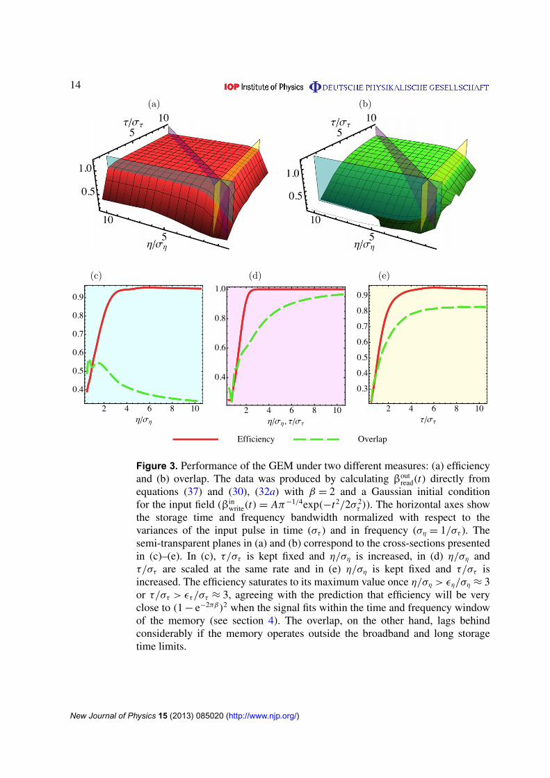
We now use the exact transfer equations to analyse the efficiency and overlap for the GEM.The results are shown in figure 3. We assumed an initial Gaussian input pulse described by thevariances στ and ση in time and frequency, respectively. The memory performance will dependon how well this input pulse fits the memory characteristics. For this reason, the importantquantities to be considered are the ratios between the memory bandwidth η and ση, and thewriting time τ and στ . In figure 3(a) we plot the efficiency as a function of these ratios.Figures 3(c), (e) and (d) show cross-sections of figures 3(a) and (b) for fixed values of τ , η andthe product τη, respectively. We see that the more the pulse fits in the memory bandwidth andstorage time, the more efficient the memory becomes. This is consistent with previous analysisof GEM in the broadband limit [28]. What is important to note here is that our analytical solutionallows us to probe the inefficiencies of the memory in regions of parameters previously onlyaccessible through numerical simulations.
The efficiency is not the only measure that must be maximized, overlap is important aswell. The overlap, depicted in figure 3(b), is consistently lower than the efficiency. It only getsclose to one for very large bandwidths and storage times and typically lags behind the efficiency.This demonstrates that the memory has caused a phase mismatch between the input and outputpulse.
We emphasize at this point that, although it is important to maximize both overlap andefficiency, a low overlap is typically much easier to correct for than a low efficiency. To correctfor a low efficiency the output signal would need to be amplified, if performed deterministicallythis process would irreversibly introduce extra noise into the signal. A low overlap on the otherhand is due to a mismatch of phase. As long as this phase mismatch can be characterizedaccurately it can be corrected for deterministically without the addition of any extra noise tothe system.
Characterization of this phase mismatch can be achieved using the analytic solution wehave provided. At the moment this phase mismatch looks like it could depend on preciselywhat input signal was received. This would make correcting it very difficult if not impossible.Fortunately we will find that in many relevant limits the phase change by the GEM isindependent of the input signal. Making it much easier to correct for.
4. Quantum memory operation: approximate analysis in the time domain
Even though our exact analytical solutions allowed us to give a complete picture of the memoryperformance as shown in figure 3, at first they look too complicated to provide any insight aboutthe physics underlying GEM. In this section, however, we will revisit our solutions for the writeand read stages to show that they can be used to understand the basic principles of quantummemories, their limitations, the different working regimes and the approximations behind them.
4.1. Basic assumptions
Now we will consider that the input pulse is limited in both time and frequency such that
βinwrite(t) ≈ 0 when t< − ετ or t>ετ (52)
New Journal of Physics 15 (2013) 085020 (http://www.njp.org/)
14
Figure 3. Performance of the GEM under two different measures: (a) efficiencyand (b) overlap. The data was produced by calculating βout
read(t) directly fromequations (37) and (30), (32a) with β = 2 and a Gaussian initial conditionfor the input field (βin
write(t) = Aπ−1/4exp(−t2/2σ 2τ )). The horizontal axes show
the storage time and frequency bandwidth normalized with respect to thevariances of the input pulse in time (στ ) and in frequency (ση = 1/στ ). Thesemi-transparent planes in (a) and (b) correspond to the cross-sections presentedin (c)–(e). In (c), τ/στ is kept fixed and η/ση is increased, in (d) η/ση andτ/στ are scaled at the same rate and in (e) η/ση is kept fixed and τ/στ isincreased. The efficiency saturates to its maximum value once η/ση > εη/ση ≈ 3or τ/στ > ετ/στ ≈ 3, agreeing with the prediction that efficiency will be veryclose to (1 − e−2πβ)2 when the signal fits within the time and frequency windowof the memory (see section 4). The overlap, on the other hand, lags behindconsiderably if the memory operates outside the broadband and long storagetime limits.
New Journal of Physics 15 (2013) 085020 (http://www.njp.org/)
15
and
βinwrite(ω) ≈ 0 when ω< − εη or ω>εη. (53)
We will also make the assumption
|(τ − ετ )(η − εη)| � 1 (54)
which allows us to approximate the Laguerre functions, as detailed in appendix C, to obtain, forthe write stage,
αoutwrite(ξ) = χ(β)
∫ τ
−τ
dt e−iξ(τ−t)−iβ ln(τ−t)(η+ξ)βinwrite(t). (55)
Here χ(β) = i√
β e−πβ/2
0(1−iβ)and therefore
|χ(β)|2 =1 − e−2πβ
2π. (56)
Looking closely to equation (55), we can see that the term e−iξ(τ−t), that would correspondto a Fourier transform, is accompanied by a logarithm term that produces a nonlinear timeand frequency dependent phase shift. This factor complicates the analysis but is also the keysignature that our solution goes beyond the broadband approximation.
For the read stage, under assumption (54) we can approximate the solution as
βoutread(t) = χ(β)
∫ η
−η
dξ eiξ(τ−t)−iβ ln(τ−t)(η−ξ)αinread(ξ). (57)
We see again the logarithm term alongside a Fourier-like term. This time, however, we also havethe memory bandwidth governing how close to a Fourier transform this term actually is.
4.2. Efficiency
We now use the approximations introduced in the previous section to estimate the efficiencyE . To begin the analysis, let us look at the total excitation stored in the material, E store
write definedby (44). This is given by
E storewrite = |χ(β)|2
∫ η
−η
dξ
∫ τ
−τ
dt ′
∫ τ
−τ
dt e−iξ(t ′−t)−iβ ln(
(τ−t ′)(τ−t)
)βin
write(t′)∗βin
write(t). (58)
In view of assumptions (52) and (53) we can extend the limits in the integrals to infinity toobtain
E storewrite ≈ (1 − e−2πβ)E in
write. (59)
In this approximation, the effect of the phase factor is simply to add a windowing effect:the memory absorbs in the window of the time it was stored, attenuated by the factor 2π |χ(β)|2.
Next, the total output energy is given by
Eoutread =
∫∞
−∞
dt ′|βout
read(t′)|2 ≈
∫ τ
−τ
dt ′|βout
read(t′)|2
= |χ(β)|2∫ τ
−τ
dt ′
∫ η
−η
dξ ′
∫ η
−η
dξ ei(τ−t ′)(ξ ′−ξ)−iβ ln
((η−ξ ′)(η−ξ)
)αin
read†(ξ)αin
read(ξ′)
= 2π |χ(β)|2∫ η
−η
dξ |αinread(ξ)|2
= 2π |χ(β)|2 E storewrite, (60)
New Journal of Physics 15 (2013) 085020 (http://www.njp.org/)

16
where in the first line we assumed that the output signal fits within the writing time window,equation (52). Note that we do not necessarily assume that the input signal is stored in a muchlarger time than its width in time. We see that the excitation of the system will come out withthe same attenuation factor as before. Now, If we use assumption (53) that the input and outputpulses fit within the bandwidth of the memory we find
Eoutread ≈ (1 − e−2πβ)2 E in
write. (61)
Consequently we find that the efficiency is given approximately by
E ≈ (1 − e−2πβ)2. (62)
We should emphasize that this is only valid when the input and output pulses fit well within thebandwidth of the system. Otherwise, the system will filter out parts of the input pulse that lieoutside its bandwidth (this is discussed further in section 5.1 below).
4.3. Long write limit
We now make the stronger assumption that the write time is much larger than the pulse width
τ � ετ . (63)
This assumption will allow us to understand the operation of the GEM in the long write regime.
4.3.1. Write stage. Under the long write assumption (63) we can approximate the logarithmby ln(τ − t) ≈ ln τ and write the our solution (55) as
αoutwrite(ξ) = χ(β)
∫ τ
−τ
dt ′ e−iξ(τ−t ′)−iβ ln τ(η+ξ)βinwrite(t
′). (64)
Since τ � ετ , we can extend the limits of the integral to infinity and obtain
αoutwrite(ξ) = χ(β) e−iξτ−iβ ln τ(η+ξ)βin
write(−ξ), (65)
where
βinwrite(ξ) =
∫∞
−∞
e−iξrβinwrite(r) dr (66)
is the Fourier transform of the input. Thus we can see that the excitation in the medium will havethe shape of the Fourier transform of the input pulse within the memory bandwidth. Note againthat −η < ξ < η so frequencies outside of this bandwidth will of course simply pass throughthe memory in the long term.
Equation (65) shows that the Fourier transform of the input is subject to attenuation andphase distortion. The attenuation (magnitude) is given by the constant factor
M long writewrite = |χ(β)| =
√1 − e−2πβ
2π(67)
which is consistent with the energy transfer relation (59). The phase distortion is a logarithmicfunction of the spatial variable ξ :
φlong writewrite (ξ) = −ξτ − β ln τ(η + ξ). (68)
Figure 4 shows the full transfer function as a function of the write time determined from theexact solution (32a). For large write times, the magnitude and phase of the transfer approachthe approximate values given by equations (67) and (68).
New Journal of Physics 15 (2013) 085020 (http://www.njp.org/)

17
a) b)
Figure 4. An example of the exact solution of the GEM during write stageapproaching the approximate transfer function with attenuation (67) (a) andphase distortion (68) (b). The transfunction interpretation of what is stored andread from the memory is only appropriate in approximate limits so a directcomparison with the exact solution is not technically possible. However we canstill gain a great deal of intuition by examining what is stored in the memory,αin
write, given an delta function input pulse, βinwrite(t) = δ(t). As the time stored
becomes longer, αinwrite will approach the transfer functions: as the transform of a
δ(t) function is flat, our output is essentially the transfer functions times 1. Wecan see that both the absolute value of αin
write (a) and the argument of αinwrite (b)
approach the expected approximated values in the long time limit. Note that in(b) we subtracted a constant phase across the frequencies, ητ , to both the exactand approximate limits to make the detail in the plots clearer.
4.3.2. Read stage. The read phase in the limit of long storage times is given by
βoutread(t) = χ(β)
∫ η
−η
dξ eiξ(τ−t)−iβ ln τ(η−ξ)αinread(ξ). (69)
We saw in the write stage that even though the excitation in the memory was simply related tothe Fourier transform of the input pulse, because the system will only absorb frequencies withinits bandwidth, the output pulse will not necessarily recreate the input pulse perfectly in time. Toanalyse the output pulse, let us look at it in Fourier space. For −η < ξ < η, we have
βoutread(ξ) = 2πχ(β)
∫ η
−η
dξ ′δ(ξ ′ + ξ) eiτξ ′−iβ ln τ(η−ξ)αin
read(ξ′)
= 2πχ(β) eiτξ−iβ ln τ(η−ξ)αinread(−ξ). (70)
This equation displays the attenuation and phase distortion during the read phase. Explicitly, theattenuation (magnitude) of the read transfer is given by
M long writeread = 2π
√1 − e−2πβ
2π(71)
and the corresponding phase is
φlong writeread (ξ) = τξ − β ln τ(η − ξ). (72)
This result is essentially the same as for the write stage, with just with a change of signs in theξ terms in the phase response corresponding to the gradient flip.
New Journal of Physics 15 (2013) 085020 (http://www.njp.org/)

18
Note that these results apply for −η < ξ < η, the detuning range of the GEM. Within thisrange, equation (70) says that in Fourier ξ -space, the output equals the internal storage up toattenuation and phase distortion factors. If we were to define ξ outside the spatial range ofthe GEM, then equation (70) would give βout
read(ξ) = 0, corresponding to a window effect in theFourier domain.
4.3.3. The whole memory process: write and read stages combined. We can now combineboth stages and analyse the full memory cycle. The total attenuation and phase distortion maybe obtained by combining the contributions from the write and read stages:
M long writewrite–read = M long write
write M long writeread
= 2π |χ(β)|2 = 1 − e−2πβ (73)
and
φlong writewrite–read(ξ) = φ
long writewrite (ξ) + φ
long writeread (ξ)
= − 2β ln τ(η + ξ)(η − ξ). (74)
This can be seen from (70) and (65)
βoutread(ξ) = χ(β) eiξ(τ−t)−iβ ln τ(η−ξ)αin
read(−ξ)
= χ(β)2 eiξ(τ−t)−iβ ln τ(η−ξ) e−iξτ−iβ ln τ(η+ξ)βinwrite(ξ) (75)
= 2πχ(β)2 e−i2β ln τ(η+ξ)(η−ξ)βinwrite(−ξ).
This equation is valid only between −η < ξ < η, outside this region βoutread(ξ) = 0. The output
emerging from the write–read cycle in the freqency domain approximately equals the input upto attenuation and phase distortion factors. In the time domain the input and output fields maynot necessarily match well.
To investigate the validity of these approximations, we look again at the exact solution. Wehave shown that in the limit of long storage time the power spectrum of the output field is thesame as in the input field within the bandwidth of the memory. Both the efficiency and overlaphave stronger requirements than just this to achieve a value of 1, so neither are good indicatorsof the approximations we have applied in this chapter being valid. So we now introduce a newmeasure, the frequency domain shape overlap (FDSO),
Oω =|∫
∞
−∞dω|βout
read(ω) ‖ βinwrite(ω) ‖
2∫∞
−∞dω|βout
read(ω)|2∫
∞
−∞dω|βin
write(ω)|2, (76)
This measures how well the shape of the power spectra of the input and output fields match. It iseasy to show that when we replace our approximate solution, equation (75), into equation (76)we get Oω = 1. Figure 5(a) shows Oω calculated from the exact solution as a function of thewriting time and bandwidth for the same set of parameters of figure 3. The growth of the FDSOin figure 5(e) confirms that the results we have derived in this section are valid in the longstorage time limit.
4.4. Broadband limit
In order to study the behaviour of a broadband memory, in place of assumption (63) we nowassume
η � εη, (77)
New Journal of Physics 15 (2013) 085020 (http://www.njp.org/)
19
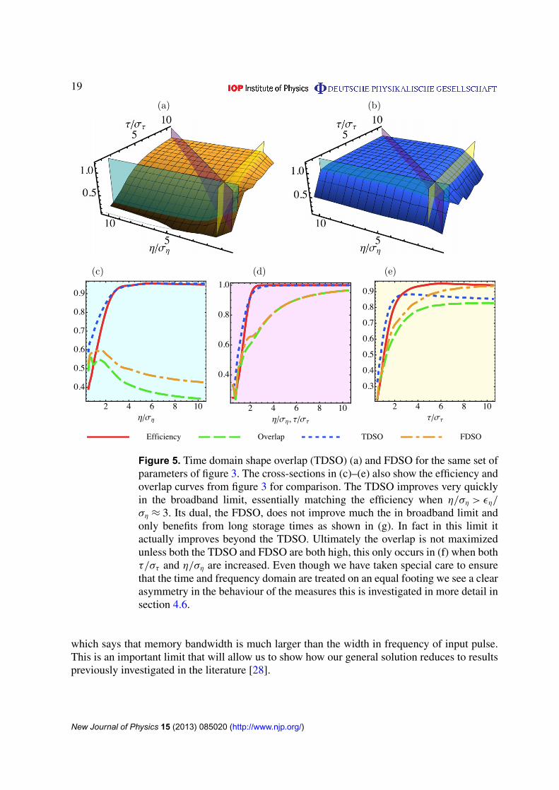
Figure 5. Time domain shape overlap (TDSO) (a) and FDSO for the same set ofparameters of figure 3. The cross-sections in (c)–(e) also show the efficiency andoverlap curves from figure 3 for comparison. The TDSO improves very quicklyin the broadband limit, essentially matching the efficiency when η/ση > εη/
ση ≈ 3. Its dual, the FDSO, does not improve much the in broadband limit andonly benefits from long storage times as shown in (g). In fact in this limit itactually improves beyond the TDSO. Ultimately the overlap is not maximizedunless both the TDSO and FDSO are both high, this only occurs in (f) when bothτ/στ and η/ση are increased. Even though we have taken special care to ensurethat the time and frequency domain are treated on an equal footing we see a clearasymmetry in the behaviour of the measures this is investigated in more detail insection 4.6.
which says that memory bandwidth is much larger than the width in frequency of input pulse.This is an important limit that will allow us to show how our general solution reduces to resultspreviously investigated in the literature [28].
New Journal of Physics 15 (2013) 085020 (http://www.njp.org/)
20
Under assumption (77) the equations for the envelopes become
αoutwrite(ξ) = χ(β)
∫ τ
−τ
dt e−iξ(τ−t)−iβ ln(τ−t)ηβinwrite(t), (78)
βoutread(t) = χ(β)
∫ η
−η
dξ eiξ(τ−t)−iβ ln(τ−t)ηαinread(ξ). (79)
These are in agreement with the analysis performed by Longdell et al [28]. Note the similaritybetween these equations and (64) and (69). In our analysis we can clearly see that the longwriting time approximation and the broadband one act as the dual of one another. This will befurther emphasized as we look at the read and write stages.
4.4.1. Write stage. Because we are assuming the broadband limit but not necessarily the longwriting time limit, it turns out that what is stored is not the Fourier transform of the input. This isdue to the t dependent logarithmic term in equation (78). Nevertheless, we may take the inverseFourier transform
αoutwrite(t) =
1
2π
∫∞
−∞
eiξ tαoutwrite(ξ) dξ (80)
to find that the overlap of the input pulse is of a high quality. Explicitly,
αoutwrite(t) = χ(β)
∫∞
−∞
dξ
∫ τ
−τ
dt ′ e−iξ(τ−t ′−t)−iβ ln(τ−t ′)ηβinwrite(t
′)
= 2πχ(β)
∫ τ
−τ
dt ′δ(τ − t ′− t) e−iβ ln(τ−t ′)ηβin
write(t′) (81)
=
{2πχ(β) e−iβ ln tηβin
write(τ − t), −τ<t<τ,
0, t< − τ or t>τ.
Consequently for −τ < t < τ the transfer to the internal storage has attenuation (magnitude)
Mbroadbandwrite = 2π |χ(β)| =
√1 − e−2πβ (82)
and phase
φbroadbandwrite = −β ln tη. (83)
We see again the attenuation factor and a windowing effect similar to what we saw before. Thistime there is a window with regard to the input pulse time, rather than a frequency filter.
4.4.2. Read stage. Much like in the previous sections, we look at the attenuation and phasedistortion. Under the broadband assumption we have
βoutread(t) = χ(β) e−iβ ln(τ−t)ηαin
read(τ − t) (84)
and so the attenuation and phase are given by
Mbroadbandread = |χ(β)| =
√1 − e−2πβ
2π(85)
and
φbroadbandread (ξ) = −β ln(τ − t)η. (86)
These relations are valid inside the time window −τ < t < τ . We see that only the light inputwithin the writing window will be stored and retrieved.
New Journal of Physics 15 (2013) 085020 (http://www.njp.org/)

21
4.4.3. The whole memory process: write and read stages combined. We can now combineboth stages and analyse the full memory cycle under the broadband assumption (77). Indeed, itfollows immediately from equations (81) and (84) that
βoutread(t) = 2πχ(β)2 e−i2β ln(τ−t)ηβin
write(t). (87)
The total attenuation and phase distortion are given by
Mbroadbandwrite–read = 2π |χ(β)|2 = 1 − e−2πβ (88)
and
φbroadbandwrite–read(t) = −2β ln(τ − t)η. (89)
We see that the output signal is identical to the input field up to the phase factor. The phasefactor means that the same may not necessarily be true in the frequency domain. We see thatthe long time limit approximation and broadband approximation are the dual of one another. Inthe long storage time domain limit the power spectrum of input signal is accurately reproducedin the output signal within the bandwidth of the memory. In the broadband case the oppositeoccurs, instead the intensity over time is reproduced accurately within the storage time windowof the memory.
We again use the exact solutions to investigate this approximation. We have shown that theintensity of the output field over time will perfectly match the intensity of the input field, up toan attenuation factor. Both the efficiency and overlap have stronger requirements than just thisto achieve a value of 1, so neither are good indicators of the approximations we have applied inthis section being valid. So we introduce a new measure the TDSO,
Ot =|∫
∞
−∞dt |βout
read(t) ‖ βinwrite(t) ‖
2∫∞
−∞dt |βout
read(t)|2∫
∞
−∞dt |βin
write(t)|2, (90)
which gives a measure of how correct we get the shape of the output beam in the timedomain. It is easy to show that when we replace our approximated solution, equation (87), intoequation (90) we get Ot = 1. The behaviour of the TDSO obtained from the analytical solutioncan be seen in figure 5(b) and the corresponding cross-sections in figures 5(c)–(e). The resultin figure 5(c) shows a complementary behaviour of the TDSO as compared to FDSO: as weapproach the broadband limit, the shape of the output signal improves but only does so in thetime domain.
4.5. Broadband and long storage time approximations
Now we will consider the limit underlying most of the intuitive understanding of GEM describedin the literature in terms of Fourier transform. If we consider both the long writing time andbroadband limits, the time domain transfer functions reduce to
αoutwrite(ξ) = χ(β) e−iβ ln τη
∫∞
−∞
dt e−iξ(τ−t)βinwrite(t), (91)
βoutread(t) = χ(β) e−iβ ln τη
∫∞
−∞
dξ eiξ(τ−t)αinread(ξ), (92)
where we have taken the limits to infinity as the input pulse will be well within the input timeand bandwidth of the memory. We can see in this limit the read and write transforms become
New Journal of Physics 15 (2013) 085020 (http://www.njp.org/)

22
true Fourier transforms up to attenuation and phase factors. Indeed, combining these expressionswe see that
βoutread(t) = 2πχ(β)2 e−i2β ln τηβin
write(t). (93)
The total attenuation and phase distortion assuming both long write and broadband assumptionsare given by
M long, broadwrite–read = 2π |χ(β)|2 = 1 − e−2πβ (94)
and
φlong, broadwrite–read (t) = −2β ln τη. (95)
As the phase factor is just a function of system parameters it can be easily cancelled outat the end with a phase plate. Assuming this is implemented we find that the overlap of theinput and output pulses of the quantum memory will approach 100% as shown in figure 5(d).In this plot η/ση and τ/στ are increased at the same rate and when large enough, all the overlapmeasures approach the efficiency curve.
4.6. Broadband versus long storage time
Even though their derivations were nearly identical and they were considered as dualapproximations, the broadband and long storage time approximations show quite distinctconvergences. Indeed, the plots in figure 5 show that the shape overlap in the time domainincreases extremely rapidly compared to the frequency domain.
Comparing equations (64) and (69) with (78) and (79), we see that the only importantdifference between them is the phase distortion factor. While the time has a (τ − t) factor inboth equations frequency has a (η − ξ) then (η + ξ). If we examine the full transfer from theinput field to the output field we get
βoutread(t) = χ2(β)
∫ η
−η
dξ
∫ τ
−τ
dt ′ e−iξ(t ′−t)−iβ ln(τ 2−(t+t ′)τ+t t ′)−iβ ln(η2/4−ξ2)βin
write(t). (96)
We note that the phase distortion is of a different order in each term. The time factor is of theorder ετ/τ while the frequency one is of the order (εη/η)2. This means that the broad bandapproximation converges much quicker than the long time approximation.
However this effect can be reduced if the signal is put through the memory twice, a strategyalready recognized in [28, 40] as a way to improve the overlap. As we have flipped the transferfunctions on the first pass, a second pass will lead to
βoutread(t) = χ4(β)
∫ η
−η
dξ1
∫ η
−η
dξ2
∫ τ
−τ
dt1
∫ τ
−τ
dt2βinwrite(t2)
×e−iξ1(t1−t)−iξ2(t2−t1)−iβ ln(τ−t1)2(τ+t2)2(η−ξ1)2(η+ξ2)
2, (97)
where now the time and frequency terms are of the same order. We can see the effect that thishas on the overlap in figure 6. Here, in contrast to figure 5(d), the overlap, efficiency,TDSO andFDSO all increase at almost the same rate, making the long time and broadband approximationstruly equivalent.
New Journal of Physics 15 (2013) 085020 (http://www.njp.org/)
23
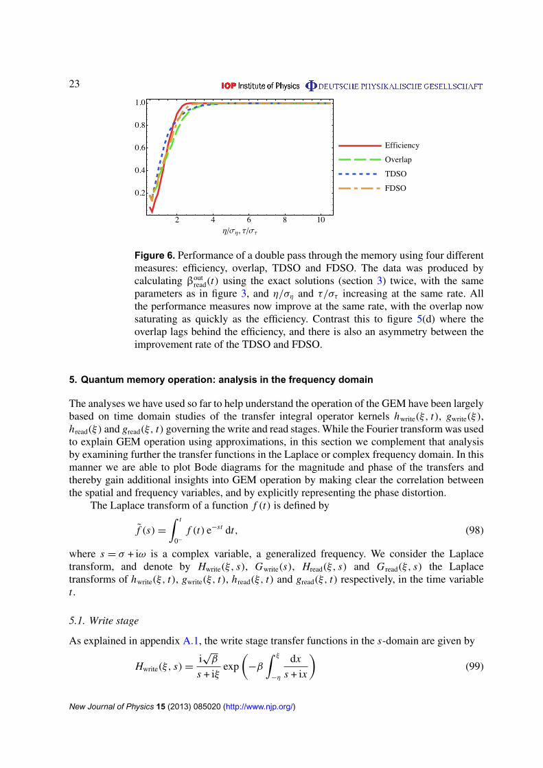
Figure 6. Performance of a double pass through the memory using four differentmeasures: efficiency, overlap, TDSO and FDSO. The data was produced bycalculating βout
read(t) using the exact solutions (section 3) twice, with the sameparameters as in figure 3, and η/ση and τ/στ increasing at the same rate. Allthe performance measures now improve at the same rate, with the overlap nowsaturating as quickly as the efficiency. Contrast this to figure 5(d) where theoverlap lags behind the efficiency, and there is also an asymmetry between theimprovement rate of the TDSO and FDSO.
5. Quantum memory operation: analysis in the frequency domain
The analyses we have used so far to help understand the operation of the GEM have been largelybased on time domain studies of the transfer integral operator kernels hwrite(ξ, t), gwrite(ξ),hread(ξ) and gread(ξ, t) governing the write and read stages. While the Fourier transform was usedto explain GEM operation using approximations, in this section we complement that analysisby examining further the transfer functions in the Laplace or complex frequency domain. In thismanner we are able to plot Bode diagrams for the magnitude and phase of the transfers andthereby gain additional insights into GEM operation by making clear the correlation betweenthe spatial and frequency variables, and by explicitly representing the phase distortion.
The Laplace transform of a function f (t) is defined by
f (s) =
∫ t
0−
f (t) e−st dt, (98)
where s = σ + iω is a complex variable, a generalized frequency. We consider the Laplacetransform, and denote by Hwrite(ξ, s), Gwrite(s), Hread(ξ, s) and Gread(ξ, s) the Laplacetransforms of hwrite(ξ, t), gwrite(ξ, t), hread(ξ, t) and gread(ξ, t) respectively, in the time variablet .
5.1. Write stage
As explained in appendix A.1, the write stage transfer functions in the s-domain are given by
Hwrite(ξ, s) =i√
β
s + iξexp
(−β
∫ ξ
−η
dx
s + ix
)(99)
New Journal of Physics 15 (2013) 085020 (http://www.njp.org/)

24
and
Gwrite(s) = exp
(−β
∫ η
−η
dx
s + ix
). (100)
It is perhaps simplest to start with the transfer function Gwrite(s), which is responsible forthe loss in the write stage and relates the input field to the output field as
βoutwrite(s) = Gwrite(s)β
inwrite(s). (101)
The time shift does not appear explicitly in equation (101) due to time invariance of the GEMduring the write stage (section 3.4).
In engineering and elsewhere, the Bode diagram is a widely used graphical representationof the frequency response of a transfer function. The frequency response concerns the behaviourof Gwrite(s) when s = iω, as ω varies over a range of frequencies. For the transfer function Gwrite
we have
Gwrite(iω) = exp
(iβ∫ η
−η
dx
ω + x
). (102)
The magnitude MGwrite(iω) and phase φGwrite(iω) are defined by
Gwrite(iω) = MGwrite(iω) eiφGwrite (iω). (103)
These may be evaluated (appendix D) to be
MGwrite(iω) =
{1 for ω > η or ω < −η,
exp(−βπ) for − η < ω < η(104)
and
φGwrite(iω) = β ln
∣∣∣∣ ω + η
ω − η
∣∣∣∣ . (105)
The Bode diagram for Gwrite(s) is shown in figure 7, where the frequency window andphase distortion can clearly be seen. Outside the frequency window, |ω| > η, all frequenciespass through. However, within the window, |ω| < η, all frequencies are attenuated by a factore−βπ , consistent with the approximate analysis given in section 4. The attenuated modes musttherefore be mostly stored, and may be called approximate dark states. Note that for the outputlight to be nearly dark there must be destructive interference between the internal and incomingcontributions, as required by the output equation (8).
We turn now to the transfer function Hwrite(ξ, s) that relates the input signal to the internalmodes
α(ξ, s) = Hwrite(ξ, s)βinwrite(s). (106)
Here, ξ ∈ (−η, η) varies over the spatial range of the GEM. The transfer function Hwrite(ξ, s)describes how the input is stored at detuning ξ . Evaluating at s = iω we have the frequencyresponse function
Hwrite(ξ, iω) =
√β
ω + ξexp
(iβ∫ ξ
−η
dx
ω + x
)(107)
= MHwrite(ξ, iω) eiφHwrite (ξ,iω), (108)
New Journal of Physics 15 (2013) 085020 (http://www.njp.org/)

25
3 2 1 0 1 2 3
3 2 1 0 1 2 30
0.5
1
ω
ω
MGwrite
φGwrite
Figure 7. Bode diagram illustrating the frequency response (magnitudeMGwrite(iω) and phase φGwrite(iω)) for the transfer function Gwrite(s). Themagnitude plot clearly shows the frequency window −η < ξ < η (with η = 1in the plots) within which the incoming modes are absorbed by the memory, andoutside of which the modes are passed through. The phase plot shows how thephase of the input is distorted as the signal is either absorbed or passed through.
and the corresponding magnitude and phase are given by
MHwrite(ξ, iω) =
√
β
|ω + ξ |for ω > η or ω < −ξ
√β
|ω + ξ |exp(−βπ) for − ξ < ω < η
(109)
and
φHwrite(ξ, iω) =
{β ln |
ω+ξ
ω−η| for ω > −ξ,
π + β ln |ω+ξ
ω−η| for ω < −ξ.
(110)
The Bode diagram for Hwrite(ξ, s) is shown in figures 8(a) and (b). The plots show themagnitude and phase as a function of the spatial variable ξ and the frequency variable ω. The‘ridge’ evident in the magnitude plot shows the correlation ξ ≈ −ω between these variables.The correlation is not perfect, as the ridge has non-zero width, and this is due to the distortionsleading to the deviations from the ideal transforms.
New Journal of Physics 15 (2013) 085020 (http://www.njp.org/)
26
a)
b)
c)
d)
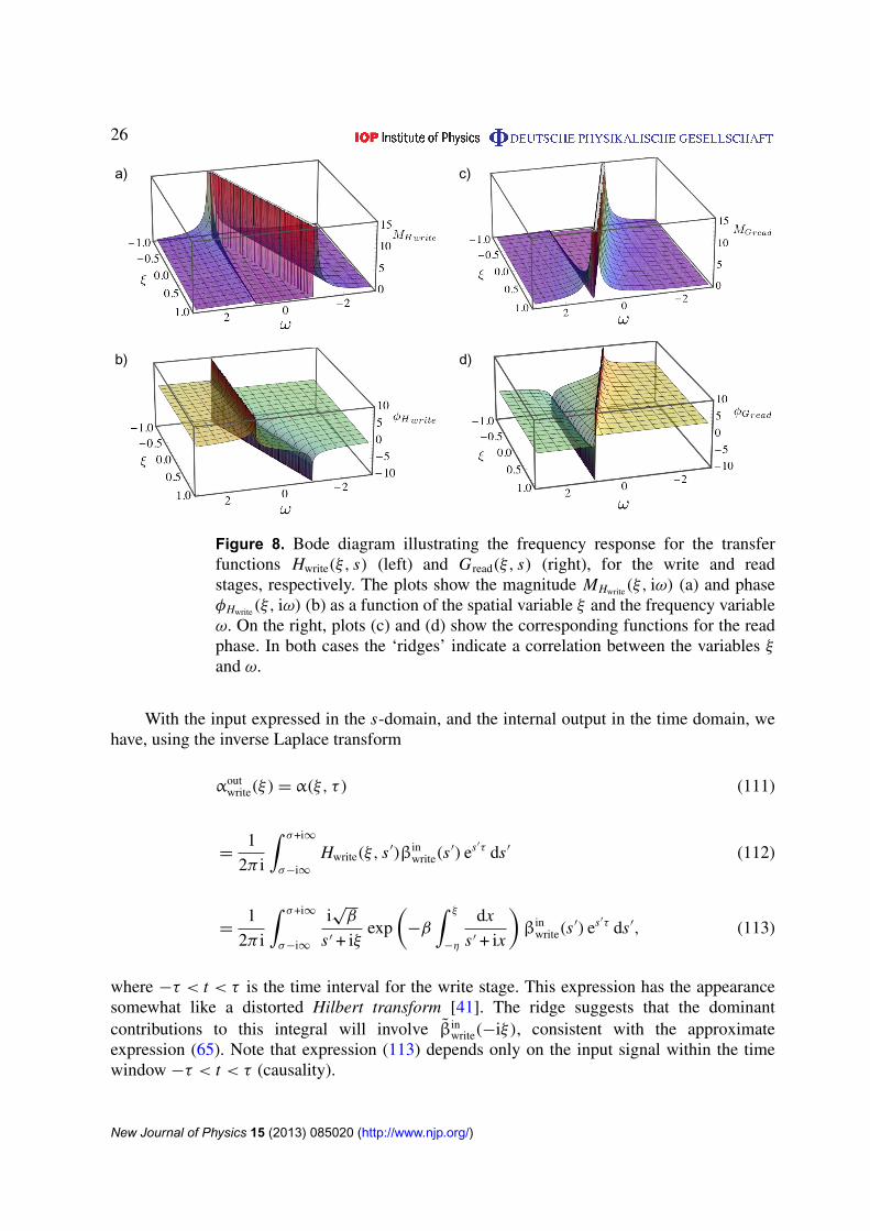
Figure 8. Bode diagram illustrating the frequency response for the transferfunctions Hwrite(ξ, s) (left) and Gread(ξ, s) (right), for the write and readstages, respectively. The plots show the magnitude MHwrite(ξ, iω) (a) and phaseφHwrite(ξ, iω) (b) as a function of the spatial variable ξ and the frequency variableω. On the right, plots (c) and (d) show the corresponding functions for the readphase. In both cases the ‘ridges’ indicate a correlation between the variables ξ
and ω.
With the input expressed in the s-domain, and the internal output in the time domain, wehave, using the inverse Laplace transform
αoutwrite(ξ) = α(ξ, τ ) (111)
=1
2π i
∫ σ+i∞
σ−i∞Hwrite(ξ, s ′)βin
write(s′) es′τ ds ′ (112)
=1
2π i
∫ σ+i∞
σ−i∞
i√
β
s ′ + iξexp
(−β
∫ ξ
−η
dx
s ′ + ix
)βin
write(s′) es′τ ds ′, (113)
where −τ < t < τ is the time interval for the write stage. This expression has the appearancesomewhat like a distorted Hilbert transform [41]. The ridge suggests that the dominantcontributions to this integral will involve βin
write(−iξ), consistent with the approximateexpression (65). Note that expression (113) depends only on the input signal within the timewindow −τ < t < τ (causality).
New Journal of Physics 15 (2013) 085020 (http://www.njp.org/)
27
5.2. Read stage
The transfer function in the s-domain for internal stored information to the output during theread stage is given by
Gread(ξ, s) =i√
β
s − iξexp
(−β
∫ η
ξ
dx
s − ix
). (114)
The frequency response is given by
Gread(ξ, iω) = MGread(ξ, iω) eiφGread (ξ,iω) (115)
and the corresponding magnitude and phase are
MGread(ξ, iω) =
√
β
|ω − ξ |for ω > η or ω < ξ,
√β
|ω − ξ |exp(−βπ) for ξ < ω < η
(116)
and
φGread(ξ, iω) =
{β ln |
ω−η
ω−ξ| for ω > ξ,
π + β ln |ω−η
ω−ξ| for ω < ξ.
(117)
The Bode diagram for Gread(ξ, s) is shown in figures 8 (c) and (d). Similar to the writestage, we see a ‘ridge’ indicating the correlation ξ ≈ ω.
The output is given by
βoutread(s) =
∫ η
−η
Gread(ξ, −s)αinread(ξ) dξ (118)
=
∫ η
−η
−i√
β
s + iξexp
(β
∫ η
ξ
dx
s + ix
)αin
read(ξ) dξ. (119)
Note that the time shift does not appear explicitly in equation (119) due to time invariance ofthe GEM during the read stage, and the minus sign in −s is due to the time reversal of the readoutput (section 3.4). Setting s = iω we have
βoutread(iω) =
∫ η
−η
−√
β
ω + ξexp
(−β
∫ η
ξ
dx
ω + x
)αin
read(ξ) dξ, (120)
and we see that the dominant contribution to the integral involves the term αinread(−iω). This
is consistent with the approximate expression (70). As for the write stage, equation (113), werecognize that the transformation appears somewhat like a distorted Hilbert transform.
6. Conclusions
We have presented and solved analytically a quantum input–output model for GEM whichmakes no assumptions on the optical depth, memory bandwidth or storage times. The model wasshown to be equivalent to previous model of memories in the weak atomic excitation regime andwe demonstrated that our general solution reduces to previous results in the appropriate limits.
New Journal of Physics 15 (2013) 085020 (http://www.njp.org/)
28
Using this solution we investigated the memory fidelity in the regime of high optical depthand finite bandwidth that maximizes efficiency in experiments. We obtained general expressionsfor several measures of storage quality due to the nonlinear phase-shifts that occur when opticaldepth is high. We also confirmed that storing a pulse twice may be used to largely undo thisshift.
The presented solution will be helpful as-is to understand and optimize high efficiencymemory experiments in the weak atomic excitation regime. The nonlinear phase-shiftinvestigated here has previously been identified as a major limiting factor for the practical use ofGEM [31]. Accurate predictions of this shift should aid general correction or accounting for it.In the long term, our model is a starting point to investigate the designing of complex networkscontaining GEM.
The presented solution should serve also as a building block to describing more complexbehaviour. It has previously been shown that manipulating the detuning gradient duringthe output stage can be used to modify the output pulse [42]. Going further than this,by incorporating a general detuning function (dependent on time and space) beyond asimple gradient, it should be possible to model general transformations on a light pulse,including correcting the nonlinear phase-shift using no external components. This would beexperimentally realizable by using complex electrode or solenoid arrangements. In this respect,our analysis in terms of transfer functions is also helpful as it establishes a strong connectionwith signal processing theory and, with it, the possibility of using the plethora of methods in thefield to manipulate the input signal via GEM. It is hoped that our approach will be accessible tothose in the signal processing field. Finally, as the model fully accounts for quantum mechanicsit will be useful for describing conditional measurements and storage of non-classical states.
Acknowledgments
We thank P K Lam, B Buchler, M Hosseini, M Sellars, K Ferguson and N Yamamoto for usefuldiscussions. We gratefully acknowledge support by the Australian Research Council Centreof Excellence for Quantum Computation and Communication Technology (project numberCE110001027) and the Air Force Office of Scientific Research (grant numbers FA2386-09-1-4089 and FA2386-12-1-4075).
Appendix A. Deriving the analytic solution
In this appendix we derive four transfer functions of the following equations:
∂tα(ξ, t) = ∓ iξα(ξ, t) + i√
ββ(ξ, t), (A.1)
∂ξβ(ξ, t) = i√
βα(ξ, t), (A.2)
which are a repeat of equations (27) and (28). We can solve these equations using a variation of aparameters method. These solutions can then be used to uniquely identify the transfer functionsin the time domain. We could have directly found the transfer functions from their LTI form,however that involves the exponentiation of an infinite dimensional matrix which can get rathertechnical.
New Journal of Physics 15 (2013) 085020 (http://www.njp.org/)
29
We will solve the system during a write then read phase each of which will go for a timeperiod of T . During the write phase we set the gradient to be positive while during the readphase we set it to be negative.
A.1. Write phase
During the write phase we will assume there is no excitation in the atoms initially, thus we canset α(ξ, 0) = 0, although the operator is non zero, any expectation value taken will be zero, sothis it is sufficient to simply apply this.
We take the Laplace transform, as defined in equation (98), of (A.1) with regard the timevariable to find
sα(ξ, s) = −iξ α(ξ, s) + i√
ββ(ξ, s), (A.3)
where we have set α(ξ, 0) = 0 during the write phase. We can rearrange (A.3) to find
α(ξ, s) =i√
β
s + iξβ(ξ, s). (A.4)
Replacing equation (A.4) into (A.2)
∂ξ β(ξ, s) =−β
s + iξβ(ξ, s). (A.5)
We can solve equation (A.4) to find
β(ξ, s) = exp
(∫ ξ
−η
dξ ′−β
s + iξ ′
)β(−η, s)
=
(s + iξ
s − iη
)iβ
β(−η, s). (A.6)
Lastly we can use a mathematical package such as Mathematica [43] and transform back to realtime to find
β(ξ, t) =
∫ t
0dt ′
(− (η + ξ)β e−iξ(t−t ′)
1 F1
(1 + iβ, 2, i(ξ + η)(t − t ′)
)+ δ(t − t ′)
)β(−η, t ′).
(A.7)
This is our first solution for equations (A.1) and (A.2). Equation (A.7) gives us the evolution ofthe outgoing light field during the write stage. In the main text this solution is presented as atransfer function in equation (31) where we define βout
write(t) = β(η, t) and βinwrite(t) = β(−η, t ′).
We can also find what quantum information is transferred on to the atoms. Replacing (A.6)into (A.4) we find
α(ξ, s) =i√
β
s + iξ
(s + iξ
s − iη
)iβ
β(−η, s). (A.8)
We can transform equation (A.8) back into the time domain and find
α(ξ, t) =
∫ t
0dt ′i
√β e−iξ(t−t ′)L
(−iβ, i(t − t ′)(ξ + η)
)β(−η, t ′). (A.9)
This is our second solution. Equation (A.9) gives us the final quantum state of the atoms afterthe write stage. In the main text this solution is presented as a transfer function in equation (30)where we define αout
write(ξ) = α(ξ, T ).
New Journal of Physics 15 (2013) 085020 (http://www.njp.org/)
30
A.2. Read phase
During the read phase we assume there is no light coming into the system so we set β(−η, t)= 0. However, now we can no longer assume that there is no excitation left in the material sowe have αin
read(ξ) = α(ξ, T ). We again solve (A.1) and (A.2) with this boundary condition anda change on the sign of the gradient.
Taking the Laplace transform of (A.1) and taking to account our changed boundaryconditions we find
sα(ξ, s) −α(ξ, T ) = iξ α(ξ, s) + i√
ββ(ξ, s). (A.10)
We can rearrange (A.10) to get
α(ξ, s) =α(ξ, T )
s − iξ+
i√
β
s − iξβ(ξ, s). (A.11)
Replacing (A.11) into (A.2) we find
∂ξ β(ξ, s) =i√
βα(ξ, T )
s − iξ−
β
s − iξβ(ξ, s). (A.12)
Equation (A.12) is an inhomogeneous differential equation which we can solve to get
β(ξ, s) =
∫ ξ
−η
dξ ′i√
β
s − iξ ′exp
(∫ ξ
ξ ′
dξ ′′−β
s − iξ ′′
)α(ξ ′, T )
=
∫ ξ
−η
dξ ′i√
β
s − iξ ′
(s − iξ ′
s − iξ
)iβ
α(ξ ′, T ). (A.13)
Where we assumed β(−η, s) = 0. We can change equation (A.13) to the time domain to get thesolution
β(ξ, t) =
∫ ξ
−η
dξ ′i√
β eiξ ′t L(−iβ, it (ξ − ξ ′)
)α(ξ ′, T ). (A.14)
This is the third solution. Equation (A.14) gives us the evolution of the outgoing light fieldduring the read stage. In the main text it is presented as a transfer function in equation (35)where βout
read(t) = β(η, t) and αinread(ξ) = α(ξ ′, T ).
Finally we can find the total excitation left in the atoms by replacing (A.13) into (A.11) tofind
α(ξ, s) =1
s − iξ
∫ ξ
−η
dξ ′
(δ(ξ − ξ ′) +
−β
s − iξ ′
(s − iξ ′
s − iξ
)iβ
α(ξ ′, T )
). (A.15)
We can equation (A.15) into the time domain to get
α(ξ, t) =
∫ ξ
−η
dξ ′
(δ(ξ − ξ ′) − (t − T )β e−i(ξ−ξ ′)(t−T )
× 1 F1
(1 + iβ, 2, i(t − T )(ξ − ξ ′)
) )α(ξ ′, T ). (A.16)
This is the fourth and final solution. Equation (A.16) gives the final quantum state of the atomsafter the read stage. In the main text is presented as a transfer function in equation (34) whereαout
read(ξ) = α(ξ, 2T ).
New Journal of Physics 15 (2013) 085020 (http://www.njp.org/)

31
Appendix B. Analytic functions
Two analytic functions form part of the analytic solution presented in this paper which arenot commonly seen. We provide their definition in terms of power series for the interestedreader, in practice they can be calculated efficiently using mathematical packages such asMathematica [43]. We define first the Kummer confluent hypergeometric function [44]
1 F1(a, b, x) =
∞∑k=0
a(n)zn
b(n)n!, (B.1)
where a(n)= a(a + 1)(a + 2) · · · (a + n − 1). This first arises while deriving the analytic solution
in equation (A.7) and is repeated in the main text in equation (32b). The other important functionis Laguerre function, which we define in terms of the Kummer confluent hypergeometric as
L(n, x) =1 F1(−n, 1, x)
0(n + 1), (B.2)
where 0(n + 1) is the Gamma function. This first arises when deriving the analytic solution inequation (A.9) and is repeated in the main text in equation (32a). When n is integer and x is realthis power series generates the well known Laguerre polynomials, however in this paper both nand x are always purely imaginary.
Appendix C. Complex Laguerre function approximation
The transformation kernel for writing the quantum information of the light onto the atomicstates (and vice versa) is difficult to analyse in its exact form. Both the write and readtransfer functions, equations (32a) and (39) respectively, contain complex Laguerre functionsof the following form L(−iβ, i(τ − t)(η ± ξ)). Fortunately the form of these kernels simplifiessignificantly in the physically relevant limit of the total time stored or the bandwidth being large.More precisely if we define 1/x = (τ − t)(η ± ξ), we find the Taylor expansion of L(−iβ, i/x)
for |x | � 1 is
L(−iβ, i/x) ≈e−πβ/2x iβ
0(1 − iβ)+ O(|x |). (C.1)
Truncating to zeroth order and replacing in our definition for x we find
L(−iβ, i(τ − t)(η ± ξ)) ≈e−πβ/2−iβ ln(τ−t)(η±ξ)
0(1 − iβ). (C.2)
This can be replaced into equations (32a) and (39) to get a much simpler transformation kernel.This form makes salient what the memories efficiency is and where the phase distortion comesfrom.
Appendix D. Magnitude and phase evaluation
Some care is required in evaluation of the magnitude and phase of the transfer functions, sinceimproper integrals and complex logarithms are involved.
We use a branch of the complex logarithm that includes the negative real line, so that,for example, ln(−1) = iπ . The reason for this is that if we carry out the integration in (102)
New Journal of Physics 15 (2013) 085020 (http://www.njp.org/)

32
we obtain formally Log(ω+η
ω−η), and the ratio ω+η
ω−ηis negative in the range −η < ω < η. So
Log(ω+η
ω−η) = ln |
ω+η
ω−η| + iπ for −η < ω < η. The magnitude and phase may also be evaluated
alternatively by an approximation involving σ + iω with σ small and positive.The attenuation is rather interesting, since each oscillator Gk in the approximating network
of section 2 is all pass, meaning |Gk(iω) = 1 for all ω. What is happening is that the poles ofeach cavity, which have strictly negative real parts, are moving in the limit to the imaginary axis,resulting in a transfer function with a continuum of purely imaginary poles.
References
[1] Lvovsky A I, Sanders B C and Tittel W 2009 Optical quantum memory Nature Photon. 3 706–14[2] Walls D F and Milburn G J 1994 Quantum Optics (Berlin: Springer)[3] Boller K J, Imamolu A and Harris S E 1991 Observation of electromagnetically induced transparency Phys.
Rev. Lett. 66 2593[4] Kraus B, Tittel W, Gisin N, Nilsson M, Kroll S and Cirac J I 2006 Quantum memory for nonstationary light
fields based on controlled reversible inhomogeneous broadening Phys. Rev. A 73 020302[5] Alexander A L, Longdell J J, Sellars M J and Manson N B 2006 Photon echoes produced by switching electric
fields Phys. Rev. Lett. 96 043602[6] Hetet G, Longdell J J, Alexander A L, Lam P K and Sellars M J 2008 Electro-optic quantum memory for
light using two-level atoms Phys. Rev. Lett. 100 023601[7] Afzelius M, Simon C, de Riedmatten H and Gisin N 2009 Multimode quantum memory based on atomic
frequency combs Phys. Rev. A 79 052329[8] McAuslan D L, Ledingham P M, Naylor W R, Beavan S, Hedges M P, Sellars M J and Longdell J J 2011
Photon-echo quantum memories in inhomogeneously broadened two-level atoms Phys. Rev. A 84 1–7[9] Damon V, Bonarota M, Louchet-Chauvet A, Chaneliere T and Le Gouet J-L 2011 Revival of silenced echo
and quantum memory for light New J. Phys. 13 093031[10] Moiseev S A and Tittel W 2011 Optical quantum memory with generalized time-reversible atom–light
interaction New J. Phys. 13 063035[11] Duan L M, Lukin M D, Cirac J I and Zoller P 2001 Long-distance quantum communication with atomic
ensembles and linear optics Nature 414 413–8[12] Ledingham P M, Naylor W R and Longdell J J 2010 Nonclassical photon streams using rephased amplified
spontaneous emission Phys. Rev. A 81 012301[13] Chaneliere T, Matsukevich D N, Jenkins S D, Lan S-Y, Kennedy T A B and Kuzmich A 2005 Storage and
retrieval of single photons transmitted between remote quantum memories Nature 438 833–6[14] Eisaman M D, Andre A, Massou F, Fleischhauer M, Zibrov A S and Lukin M D 2005 Electromagnetically
induced transparency with tunable single-photon pulses Nature 438 837–41[15] Appel J, Figueroa E, Korystov D, Lobino M and Lvovsky A I 2008 Quantum memory for squeezed light
Phys. Rev. Lett. 100 093602[16] Choi K S, Deng H, Laurat J and Kimble H J 2008 Mapping photonic entanglement into and out of a quantum
memory Nature 452 67[17] Honda K, Akamatsu D, Arikawa M, Yokoi Y, Akiba K, Nagatsuka S, Tanimura T, Furusawa A and Kozuma M
2008 Storage and retrieval of a squeezed vacuum Phys. Rev. Lett. 100 093601[18] Longdell J J, Fraval E, Sellars M J and Manson N B 2005 Stopped light with storage times greater than one
second using electromagnetically induced transparency in a solid Phys. Rev. Lett. 95 063601[19] Hedges M P, Longdell J J, Li Y and Sellars M J 2010 Efficient quantum memory for light Nature 465 1052–6[20] Hosseini M, Sparkes B M, Campbell G, Lam P K and Buchler B C 2011 High efficiency coherent optical
memory with warm rubidium vapour Nature Commun. 2 174
New Journal of Physics 15 (2013) 085020 (http://www.njp.org/)

33
[21] Hosseini M, Campbell G, Sparkes B M, Lam P K and Buchler B C 2011 Unconditional room-temperaturequantum memory Nature Phys. 7 794–8
[22] Clausen C, Usmani I, Bussieres F, Sangouard N, Afzelius M, de Riedmatten H and Gisin N 2011 Quantumstorage of photonic entanglement in a crystal Nature 469 508–11
[23] Saglamyurek E, Sinclair N, Jin J, Slater J A, Oblak D, Bussieres F, George M, Ricken R, Sohler W andTittel W 2011 Broadband waveguide quantum memory for entangled photons Nature 469 512–5
[24] Radnaev A G, Dudin Y O, Zhao R, Jen H H, Jenkins S D, Kuzmich A and Kennedy T A B 2010 A quantummemory with telecom-wavelength conversion Nature Phys. 6 894–9
[25] Alexander A L 2007 Investigation of quantum information storage in rare earth doped materials PhD ThesisAustralian National University
[26] Hetet G, Hosseini M, Sparkes B M, Oblak D, Lam P K and Buchler B C 2008 Photon echoes generated byreversing magnetic field gradients in a rubidium vapor Opt. Lett. 33 2323–5
[27] Hosseini M, Sparkes B M, Hetet G, Longdell J J, Lam P K and Buchler B C 2009 Coherent optical pulsesequencer for quantum applications Nature 461 241–5
[28] Longdell J J, Hetet G, Lam P K and Sellars M J 2008 Analytic treatment of controlled reversibleinhomogeneous broadening quantum memories for light using two-level atoms Phys. Rev. A 78 032337
[29] Hetet G, Longdell J J, Sellars M J, Lam P K and Buchler B C 2008 Multimodal properties and dynamics ofgradient echo quantum memory Phys. Rev. Lett. 101 203601
[30] Nunn J, Reim K, Lee K C, Lorenz V O, Sussman B J, Walmsley I A and Jaksch D 2008 Multimode memoriesin atomic ensembles Phys. Rev. Lett. 101 260502
[31] Moiseev S A and Arslanov N M 2008 Efficiency and fidelity of photon-echo quantum memory in an atomicsystem with longitudinal inhomogeneous broadening Phys. Rev. A 78 023803
[32] Gardiner C W and Zoller P 2004 Quantum Noise 3rd edn (Berlin: Springer)[33] Gardiner C W 1993 Driving a quantum system with the output field from another driven quantum system
Phys. Rev. Lett. 70 2269–72[34] Carmichael H J 1993 Quantum trajectory theory for cascaded open systems Phys. Rev. Lett. 70 2273–6[35] Gough J and James M R 2009 The series product and its application to quantum feedforward and feedback
networks Autom. Control IEEE Trans. 54 2530–44[36] Protsenko I, Domokos P, Lefevre-Seguin V, Hare J, Raimond J M and Davidovich L 1999 Quantum theory of
a thresholdless laser Phys. Rev. A 59 1667–82[37] Carmichael H J 1993 An Open Systems Approach to Quantum Optics (Berlin: Springer)[38] Kailath T 1980 Linear Systems (Englewood Cliffs, NJ: Prentice-Hall)[39] Bouten L, Van Handel R and James M 2007 An introduction to quantum filtering SIAM J. Control Optim.
46 2199–241[40] Hetet G 2008 Quantum memories for continuous variable states of light in atomic ensembles PhD Thesis
Australian National University Canberra[41] Bracewell R N 1986 The Fourier Transform and its Applications 2nd edn (New York: McGraw-Hill)[42] Buchler B C, Hosseini M, Hetet G, Sparkes B M and Lam P K 2010 Precision spectral manipulation of optical
pulses using a coherent photon echo memory Opt. Lett. 35 1091–3[43] (Wolfram Research) 2012 Mathematica version 9.0 ed (Champaign, IL: Wolfram Research, Inc.)[44] Abramowitz M and Stegun I A (ed) 1972 Handbook of Mathematical Functions with Formulas, Graphs
and Mathematical Tables 10th printing edn (Washington, DC: Department of Commerce United States ofAmerica) p 504
New Journal of Physics 15 (2013) 085020 (http://www.njp.org/)