Analysis of the Mixing of Solid Particles in the Slant

Cone and Ploughshare Mixers via Discrete Element

Method (DEM)

by

Seyed-Meysam Seyed-Alian

B.Sc., Amirkabir University of Technology, Tehran, Iran, 2011

A Thesis

Presented to Ryerson University

in Partial Fulfillment of the Requirements for the Degree of

Master of Applied Science

in the Program of Chemical Engineering

Toronto, Ontario, Canada, 2013

Copyright © 2013 by Seyed-Meysam Seyed-Alian

ii

AUTHOR’S DECLARATION FOR ELECTRONIC

SUBMISSION OF A THESIS

I hereby declare that I am the sole author of this thesis. This is a true copy of

the thesis, including any required final revisions, as accepted by my

examiners.

I authorize Ryerson University to lend this thesis to other institutions or

individuals for the purpose of scholarly research.

I further authorize Ryerson University to reproduce this thesis by

photocopying or by other means, in total or in part, at the request of other

institutions or individuals for the purpose of scholarly research.

I understand that my thesis may be made electronically available to the

public.

iii

ABSTRACT

Seyed-Meysam Seyed-Alian

Analysis of the Mixing of Solid Particles in the Slant Cone and

Ploughshare Mixers via Discrete Element Method (DEM)

M.A.Sc, Chemical Engineering, Ryerson University, Toronto, 2013

Discrete element method (DEM) was employed to characterize the mixing of the solid

particles in two different types of the powder blenders. In the first part of this study, DEM

was used to investigate the effects of initial loading, drum speed, fill level, and agitator

speed on the mixing efficiency of a slant cone mixer. DEM simulation results were in

good agreement with the experimentally determined data, both qualitatively and

quantitatively. In the second part of this study, DEM was employed to characterize the

mixing of the solid particles in a Ploughshare mixer. To validate the model, the

simulation results were compared to the positron emission particle tracking (PEPT) data

reported in the literature. The validated DEM was then utilized to calculate the mixing

index as a function of the initial loading, plough rotational speed, fill level, and particle

size for a ploughshare mixer.

iv

Acknowledgement

I would first like to express my sincere gratitude and appreciation on my supervisors

Dr. Farhad Ein-Mozaffari and Dr. Simant Upreti for their guidance and encouraging

enthusiasm during all times of this work.

I acknowledge the assistance of all the staff and technologists in the Chemical

Engineering Department at Ryerson University.

I also would like to acknowledge the advice and helpful suggestion of my friends (Bahar

Abghari, Amir Mowla, Navid Hakimi, Leila Pakzad, Samin Eftekhari and …) in the Fluid

Mixing Technology Laboratory at Ryerson University.

I would like to thank Cosmetica Laboratories Inc. for providing the slant cone mixer.

Financial support from Natural Sciences and Engineering Research Council of Canada

(NSERC) is gratefully acknowledged.

v

This thesis is dedicated to my parents whose love, guidance, and sacrifice

have made me the person I am today.

vi

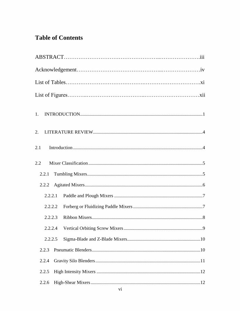
Table of Contents

ABSTRACT……………………………………………..………………….iii

Acknowledgement………………………………………..…………………iv

List of Tables…………………………………….………………………….xi

List of Figures………..…………………………..…………………………xii

1. INTRODUCTION........................................................................................................ 1

2. LITERATURE REVIEW ............................................................................................. 4

2.1 Introduction .............................................................................................................. 4

2.2 Mixer Classification ................................................................................................. 5

2.2.1 Tumbling Mixers .................................................................................................. 5

2.2.2 Agitated Mixers .................................................................................................... 6

2.2.2.1 Paddle and Plough Mixers ........................................................................... 7

2.2.2.2 Forberg or Fluidizing Paddle Mixers ........................................................... 7

2.2.2.3 Ribbon Mixers .............................................................................................. 8

2.2.2.4 Vertical Orbiting Screw Mixers ................................................................... 9

2.2.2.5 Sigma-Blade and Z-Blade Mixers .............................................................. 10

2.2.3 Pneumatic Blenders ............................................................................................ 10

2.2.4 Gravity Silo Blenders ......................................................................................... 11

2.2.5 High Intensity Mixers ........................................................................................ 12

2.2.6 High-Shear Mixers ............................................................................................. 12

vii

2.3 Different State of Solids Mixture ........................................................................... 13

2.4 Quantification of Solids Mixing............................................................................. 17

2.4.1 Statistical Analysis ............................................................................................. 17

2.4.1.1 Intensity of Segregation ............................................................................. 17

2.4.1.2 Relative Standard Deviation (RSD) ........................................................... 18

2.4.1.3 Mixture Variance ....................................................................................... 19

2.4.1.4 Average-Height Method ............................................................................. 21

2.4.1.5 Nearest-Neighbors Method ........................................................................ 22

2.4.1.6 Lacey’s Method .......................................................................................... 23

2.4.1.7 Neighbor-Distance Method ........................................................................ 24

2.4.2 Image Analysis ................................................................................................... 26

2.4.3 Calculation of the Mixing Time ......................................................................... 28

2.5 Different Sampling Methods .................................................................................. 29

2.5.1 Physical Sampling Methods ............................................................................... 30

2.5.1.1 Side Sampling Thief ................................................................................... 31

2.5.1.1.1 Globe-Pharma Probe ............................................................................ 32

2.5.1.1.2 Groove Thief ........................................................................................ 33

2.5.1.2 End Sampling Thief ................................................................................... 33

2.5.1.2.1 End-Cup Sampler ................................................................................. 33

2.5.1.2.2 Core Sampler ........................................................................................ 34

2.5.2 Non-Invasive Methods ....................................................................................... 34

2.6 Discrete Element Method ....................................................................................... 36

viii

2.7 Contact Force Models ............................................................................................ 41

2.7.1 Normal Contact Force Models ........................................................................... 42

2.7.1.1 Continuous Potential Contact Models: ....................................................... 42

2.7.1.2 Linear Viscoelastic Models (Linear Spring Dashpot) ................................ 43

2.7.1.3 Nonlinear Viscoelastic Models (Nonlinear Spring Damper) ..................... 45

2.7.1.4 Hysteretic Models ...................................................................................... 45

2.7.2 Tangential Force ................................................................................................. 46

2.7.2.1 Mindlin and Deresiewicz (1953) ................................................................ 46

2.8 DEM Utilized ......................................................................................................... 48

2.8.1 Tote Blender ....................................................................................................... 48

2.8.2 Paddle Mixer ...................................................................................................... 50

2.8.3 V-Blender ........................................................................................................... 51

2.8.4 Double Cone Blender ......................................................................................... 52

2.9 Research Objectives ............................................................................................... 53

3. USING DISCRETE ELEMENT METHOD TO ANALYZE THE MIXING OF THE

SOLID PARTICLES IN A SLANT CONE MIXER ......................................................... 54

3.1 Introduction ............................................................................................................ 54

3.2 Specifications of the Mixer and Experimental Methods: ....................................... 56

3.3 Discrete Element Method (DEM) .......................................................................... 61

3.4 Results and Discussion ........................................................................................... 68

ix

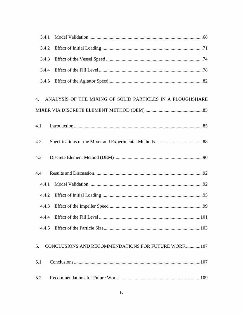
3.4.1 Model Validation ............................................................................................... 68

3.4.2 Effect of Initial Loading ..................................................................................... 71

3.4.3 Effect of the Vessel Speed ................................................................................. 74

3.4.4 Effect of the Fill Level ....................................................................................... 78

3.4.5 Effect of the Agitator Speed ............................................................................... 82

4. ANALYSIS OF THE MIXING OF SOLID PARTICLES IN A PLOUGHSHARE

MIXER VIA DISCRETE ELEMENT METHOD (DEM) ................................................ 85

4.1 Introduction ............................................................................................................ 85

4.2 Specifications of the Mixer and Experimental Methods ........................................ 88

4.3 Discrete Element Method (DEM) .......................................................................... 90

4.4 Results and Discussion ........................................................................................... 92

4.4.1 Model Validation ............................................................................................... 92

4.4.2 Effect of Initial Loading ..................................................................................... 95

4.4.3 Effect of the Impeller Speed .............................................................................. 99

4.4.4 Effect of the Fill Level ..................................................................................... 101

4.4.5 Effect of the Particle Size ................................................................................. 103

5. CONCLUSIONS AND RECOMMENDATIONS FOR FUTURE WORK ............ 107

5.1 Conclusions .......................................................................................................... 107

5.2 Recommendations for Future Work ..................................................................... 109

x

NOMENCLATURE ......................................................................................................... 110

GLOSSARY ..................................................................................................................... 112

BIBLIOGRAPHY: ........................................................................................................... 113

xi

List of Tables

Table 3.1. Parameters used in DEM simulations ............................................................... 64

Table 3.2. Variety of mixing index for mesh sizes of 10×10×10 to 30×30×30. ................ 67

Table 3.3. Total number of particles used in each simulation ........................................... 78

Table 4.1. Parameters used in the simulations. .................................................................. 90

xii

List of Figures

Figure 2.1. Distributions of individual particles that form a) perfect mixture, b) random

mixture, c) ideal ordered mixture, d) ordered mixture, e) pseudorandom mixture,

and f) textured mixtures. ...................................................................................... 16

Figure 2.2. Voigt model for (a) normal and (b) tangential direction of contact between

two particles ......................................................................................................... 39

Figure 2.3. Translational and rotational displacement for one particle in the time interval

of ..................................................................................................................... 39

Figure 2.4. Normal and tangential displacement for two particles in contact. ................... 40

Figure 2.5. Schematic of a viscoelastic model ................................................................... 44

Figure 2.6.Schematic of a hysteretic model ....................................................................... 46

Figure 3.1.Slant Cone Mixer used in this study ................................................................. 57

Figure 3.2. 3D model of the Gemco Slant cone mixer (all dimensions are in millimeters)

............................................................................................................................. 58

Figure 3.3. Intensifier bars of the slant cone mixer with T-shaped blades (all dimensions

are in millimeters) ................................................................................................ 59

Figure 3.4.(a) Thief sampler and (b) Cardboard template ................................................. 60

Figure 3.5. Schematic of the slant cone mixer with cubic cells ......................................... 65

xiii

Figure 3.6. Comparison between the Lacey index achieved through the experiment and

simulation at the fill level of 70%, the drum speed of 12.5 rpm and the side-side

initial loading while the agitator was stationary. ................................................. 69

Figure 3.7. Comparison between the snapshots of the simulated and real solid mixtures at

each revolution at the fill level of 70%, drum speed of 12.5 rpm and side-side

initial loading while the agitator was stationary. ................................................. 70

Figure 3.8. Mixing index versus time for different initial loading at the fill level of 70%

and the drum speed of 12.5 rpm while the agitator was stationary. .................... 71

Figure 3.9. Snapshots of the simulated solid mixture for the three different loading

patterns at times equal to 0, 12, and 24 s at the fill level of 70% and the drum

speed of 12.5 rpm while the agitator was stationary. .......................................... 73

Figure 3.10. Mixing index versus time for different speed of vessel at the fill level of 70%

and the side-side initial loading while the agitator was stationary. ..................... 74

Figure 3.11. Increased kinetic energy versus time at different drum speeds (green, blue

and red lines represent 20 rpm, 12.5 rpm and 5 rpm, respectively), the fill level

of 70%, and the side-side initial loading while the agitator was stationary. ....... 77

Figure 3.12. Mixing index versus time at different fill levels, the drum speed of 12.5 rpm,

and the side-side initial loading while the agitator was stationary. ..................... 79

Figure 3.13. Fill level guideline for the slant cone mixer .................................................. 81

Figure 3.14.Kinetic energy of solid particles versus time at different fill levels (green,

blue and red lines represent 100%, 70% and 30% fill level, respectively), the

xiv

drum speed of 12.5 rpm, and the side-side initial loading while the agitator was

stationary. ............................................................................................................. 81

Figure 3.15.Mixing index versus time at the different agitator speeds, the fill level of

100%, the drum speed of 12.5 rpm and the side-side initial loading while the

agitator was stationary. ........................................................................................ 83

Figure 3.16. Velocities of the particles in the slant cone mixer at the fill level of 100%,

the drum speed of 12.5 rpm, the side-side initial loading, and the agitator speed

of 200 rpm: (a) counter-rotating mode and (b) co-rotating mode. ...................... 84

Figure 4.1.The imported geometry of the ploughshare mixer for DEM simulations ........ 89

Figure 4.2. Plough dimensions in millimeters ................................................................... 89

Figure 4.3 . Schematic of the ploughshare mixer with cubic cells .................................... 91

Figure 4.4. The imported geometry of the ploughshare mixer equipped with a single

plough for DEM simulations ............................................................................... 93

Figure 4.5.Mean square of the axial displacement (mm) versus the number of blade

passes at 1Hz speed of the blade and the fill level of 25% .................................. 94

Figure 4.6. Mean square of the radical displacement (mm) versus the number of blade

passes at 1Hz speed of the blade and the fill level of 25% .................................. 95

Figure 4.7. Mixing index versus time for different initial loading methods at the fill level

of 20% and the blade speed of 90 rpm ................................................................ 96

xv

Figure 4.8. Snapshots of the simulated solid mixture at times equal to 0, 5, 10 and 15 s at

the fill level of 20% and the blade speed of 90 rpm for: (a) the side-side loading

and (b) the top-bottom loading. ........................................................................... 98

Figure 4.9. Mixing index versus time at different blade speeds, the fill level of 20%, and

the side-side initial loading ................................................................................ 100

Figure 4.10. Mixing index versus time at different fill levels, the blade speed of 90 rpm,

and the side-side initial loading ......................................................................... 102

Figure 4.11. Mixing index versus time for different particle sizes, the blade speed of 120

rpm, and the side-side initial loading ................................................................. 104

Figure 4.12. Average velocity of the particles versus time, the blade speed of 120 rpm,

and the side-side initial loading ......................................................................... 105

Figure 4.13. Average velocity of the particles versus particles size, the blade speed of 120

rpm, and the side-side initial loading ................................................................. 106

1

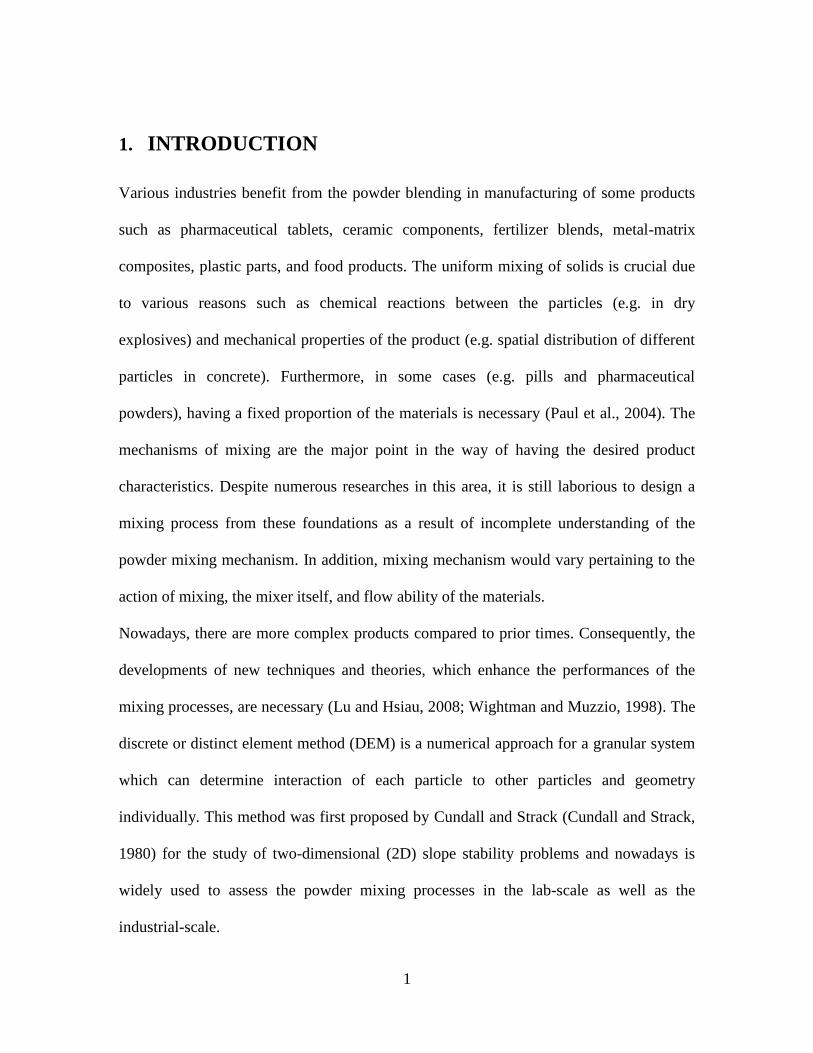
1. INTRODUCTION

Various industries benefit from the powder blending in manufacturing of some products

such as pharmaceutical tablets, ceramic components, fertilizer blends, metal-matrix

composites, plastic parts, and food products. The uniform mixing of solids is crucial due

to various reasons such as chemical reactions between the particles (e.g. in dry

explosives) and mechanical properties of the product (e.g. spatial distribution of different

particles in concrete). Furthermore, in some cases (e.g. pills and pharmaceutical

powders), having a fixed proportion of the materials is necessary (Paul et al., 2004). The

mechanisms of mixing are the major point in the way of having the desired product

characteristics. Despite numerous researches in this area, it is still laborious to design a

mixing process from these foundations as a result of incomplete understanding of the

powder mixing mechanism. In addition, mixing mechanism would vary pertaining to the

action of mixing, the mixer itself, and flow ability of the materials.

Nowadays, there are more complex products compared to prior times. Consequently, the

developments of new techniques and theories, which enhance the performances of the

mixing processes, are necessary (Lu and Hsiau, 2008; Wightman and Muzzio, 1998). The

discrete or distinct element method (DEM) is a numerical approach for a granular system

which can determine interaction of each particle to other particles and geometry

individually. This method was first proposed by Cundall and Strack (Cundall and Strack,

1980) for the study of two-dimensional (2D) slope stability problems and nowadays is

widely used to assess the powder mixing processes in the lab-scale as well as the

industrial-scale.

2

The first objective of this study is to investigate the performance of a slant cone mixer as

a function of initial loading (side-side, top-bottom, and back-front), drum speed, fill level,

and agitator speed using discrete element method (DEM). Moreover, assessing the mixing

index as a function of the initial loading, the rotational speed, fill level, and the particle

size for a six-blade ploughshare mixer through the discrete element method (DEM) is the

next objective of the current study.

Chapter two gives a brief review of literature to present the fundamental in powder

mixing such as powder mixers classification, different state and quantification of solid

mixture, different sampling method, discrete element method, and contact force models.

At the end, some DEM applications especially in mixing process are presented.

In Chapter three discrete element method (DEM) was employed to characterize the

mixing of the solid particles in a Slant cone mixer. DEM results were validated using

experimental data obtained from both sampling and image techniques. DEM simulation

results were in good agreement with the experimentally determined data, both

qualitatively and quantitatively.

Chapter four provides the information regarding assessing the mixing of the solid

particles in a Ploughshare mixer. To validate the model, the simulation results were

compared to the Positron Emission Particle Tracking (PEPT) data reported in the

literature by Laurent and Cleary (2012) for a ploughshare mixer. The simulation results

were in good agreement with the experimental data. The validated DEM was then utilized

to calculate the mixing index as a function of the initial loading, rotational speed of

impeller, fill level, and particle size for a six-blade ploughshare mixer. Moreover, the

3

mixing time, which is the time required to reach a homogeneous mixture, was presented

as a function of the operating conditions.

Eventually Chapter five summaries the overall conclusions of the present study and give

the recommendations for the future work.

4

2. LITERATURE REVIEW

2.1 Introduction

This chapter gives a brief review of literature to present the fundamental in powder

mixing such as powder mixers classification, different state and quantification of solid

mixture, different sampling method, discrete element method, and contact force models.

At the end, some DEM applications especially in mixing process are presented.

Although several works have been done on the fundamental understanding of the powder

mixing ( Langston et al., 1994, Potapov and Campbell, 1996, Rong et al., 1995, Dury and

Ristow, 1997, Muguruma et al., 1997, Matsusaka et al., 1998, Mikami et al., 1998,

Wightman et al., 1998, Vu-Quoc et al., 1999, Kaneko et al., 2000, Moakher et al., 2000,

Kuo et al., 2002, Cleary, 2000, Yamane, 2000, Hoomans et al., 2000, Mishra and Murty,

2000, Laurent and Cleary, 2006, Hanes and Walton, 2000, Rajamani et al., 2000, Shimizu

and Cundall, 2001, Rhodes et al., 2001, Venugopal and Rajamani, 2001, Stewart et al.,

2001, Iwasaki et al., 2001, Cleary and Sawley, 2002, Zhou et al., 2002, Kuo et al., 2005,

Asmar et al., 2002, Yamane., 2004, Cleary, 2004, Sudah et al., 2005, Bertrand et al.,

2005, Laurent, 2006, Arratia et al., 2006, Chaudhuri et al., 2006, Chaikittisilp et al., 2006,

Lemieux et al, 2007, Lemieux et al., 2008, Renzo et al., 2008, Lua and Hsiau, 2008,

Remy et al., 2009, Geng et al., 2009, Nakamura et al., 2009, Mio et al., 2009, Bharadwaj

et al., 2010, Sarkar and Wassgren., 2010, Manickam et al., 2010, Dubey et al., 2011,

Siiriä and Yliruusi ,2011, Hassanpour et al., 2011, Sahni et al., 2011, Sudbrock et al.,

2011, Powell et al, 2011, Marigo et al., 2012, Siraj et al, 2011, Ahmadian et al., 2011,

5

Chandratilleke and Yu., 2012, Zhu et al. 2011, Li et al, 2012), there are still uncertainties

especially in them of mixing efficiency.

2.2 Mixer Classification

Industrial mixers can be broadly classified into the following categories (Paul et al.,

2004):

Tumbling mixers: v-blender, double cone blender, tote or bin blender, slant cone

blender

Agitated mixers: paddle and plough, fluidizing paddle mixers (Forberg Mixer),

Ribbon blenders, screw mixers, sigma-blade and z-blade mixers

Pneumatic blenders

Gravity silo blenders

High-intensity mixers

High-intimacy or high-shear mixers

2.2.1 Tumbling Mixers

Multiple industries are using tumbling blenders widely in granular mixing operations,

including pharmaceutical, cosmetics, mining, food, energy, polymer, and semiconductor.

Tumbling blenders are easy to operate, available in various capacities and are able to

operate with shear sensitive or non-agglomerating materials. Their cleaning and emptying

procedures are easy. Moreover, tumbling blenders are suitable for blending of dry and

6

free flowing materials (Alexander et al., 2004; Kuo et al., 2005). Finally, the tumbling

mixers benefit from simple mixing mechanisms. A closed vessel rotates around the axis

in a tumbling mixer. Mixing in this type of blender is achieved due to the random motions

of the particles rolling down from an inclined surface. The counter rotating of the vessel

and the installation of internal baffles would also enhance the mixing of particles (Cullen,

2009). Of course there are some disadvantages on using the tumbling mixers. One of

them is the high chance of the segregation of the particles. Furthermore, mixing is

typically confined to the surface of powder bed and leaving large regions undisturbed

during long periods of the mixing cycle. In addition, tumbling mixers are not suitable for

the agglomerating particles (Cullen, 2009; Poux et al., 1991).

2.2.2 Agitated Mixers

In agitated blenders, particles are mixed mechanically in a fixed shell by using paddles,

ploughs, or ribbons. Along with the bulk mass, the mixing is achieved with the random

movements of particles in agitated mixers. In fact, the mixing is accomplished by both

convection and shear in this type of the mixers. In a common design of the agitated mixer,

the agitating tools, which are attached to a single or twin shaft, are rotated in a motionless

shell, which could be vertical or horizontal. Depending on the speed of the ploughs or

paddles, the product is mechanically sheared or fluidized and particles are tossed

randomly. The agitated mixers are frequently employed for the mixing of the solid

particles including free-flowing particles, cohesive particles, and pastes (Fuller, 1998;

Kent, 2002; Ramponi et al., 2002).

7

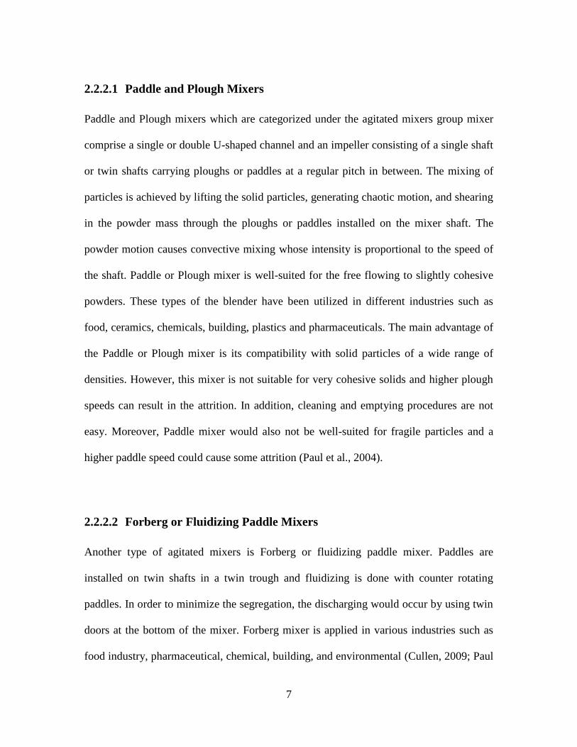
2.2.2.1 Paddle and Plough Mixers

Paddle and Plough mixers which are categorized under the agitated mixers group mixer

comprise a single or double U-shaped channel and an impeller consisting of a single shaft

or twin shafts carrying ploughs or paddles at a regular pitch in between. The mixing of

particles is achieved by lifting the solid particles, generating chaotic motion, and shearing

in the powder mass through the ploughs or paddles installed on the mixer shaft. The

powder motion causes convective mixing whose intensity is proportional to the speed of

the shaft. Paddle or Plough mixer is well-suited for the free flowing to slightly cohesive

powders. These types of the blender have been utilized in different industries such as

food, ceramics, chemicals, building, plastics and pharmaceuticals. The main advantage of

the Paddle or Plough mixer is its compatibility with solid particles of a wide range of

densities. However, this mixer is not suitable for very cohesive solids and higher plough

speeds can result in the attrition. In addition, cleaning and emptying procedures are not

easy. Moreover, Paddle mixer would also not be well-suited for fragile particles and a

higher paddle speed could cause some attrition (Paul et al., 2004).

2.2.2.2 Forberg or Fluidizing Paddle Mixers

Another type of agitated mixers is Forberg or fluidizing paddle mixer. Paddles are

installed on twin shafts in a twin trough and fluidizing is done with counter rotating

paddles. In order to minimize the segregation, the discharging would occur by using twin

doors at the bottom of the mixer. Forberg mixer is applied in various industries such as

food industry, pharmaceutical, chemical, building, and environmental (Cullen, 2009; Paul

8

et al., 2004). The effect of shear in the Forberg mixer is negligible due to meritorious

mixing quality and short time of mixing. Consequently, it is suitable for processing

friable materials adding to non-aggregating, segregating and slightly cohesive ones

(Forberg, 1992; Smith, 1997). Besides, it can be applied to coating solid particles carrying

a liquid layer. As a result of slug movements of chemicals through one or two doors with

full length located in the bottom of the mixer, the particle segregation during discharging

is extremely reduced (Vandenbergh, 1994). Paddle mixers are able to produce the

homogenous mixtures that are independent of particles size, shape and density. Also,

mixers would minimize the product degradation and have low operating costs, and they

ensure fast and yet gentle blending with short mixing cycle. However, high paddle speed

could result in attrition. This type of mixer is not designed for the fragile particles.

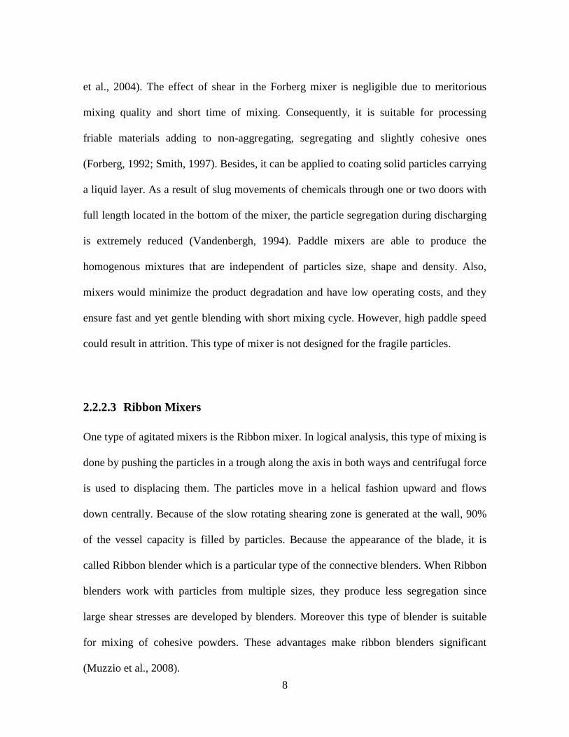
2.2.2.3 Ribbon Mixers

One type of agitated mixers is the Ribbon mixer. In logical analysis, this type of mixing is

done by pushing the particles in a trough along the axis in both ways and centrifugal force

is used to displacing them. The particles move in a helical fashion upward and flows

down centrally. Because of the slow rotating shearing zone is generated at the wall, 90%

of the vessel capacity is filled by particles. Because the appearance of the blade, it is

called Ribbon blender which is a particular type of the connective blenders. When Ribbon

blenders work with particles from multiple sizes, they produce less segregation since

large shear stresses are developed by blenders. Moreover this type of blender is suitable

for mixing of cohesive powders. These advantages make ribbon blenders significant

(Muzzio et al., 2008).

9

There are several reports that provide some basic information about helical ribbon

agitators such as the power consumption of agitators, flow pattern and mixing

characteristics. In addition to the mixing liquids of high viscosity, helical ribbons have

been applied to blend the powders (Carreau et al., 1976; Kaneko et al., 2000). The ribbon

blender is applicable for segregated and cohesive or agglomerative particles due to their

continuous rather than batch processing design. Some industries benefit from using

Ribbon blenders such as construction, agriculture, chemicals, pharmaceuticals, and foods

in order to mix powders, granular solids, slurries, liquids, pastes, cereals, plastics, and

pigments (Thyn and Duffek, 1976). However it is not suitable to use the mixers for

products with sticky characteristics. In addition, Ribbon blenders have a small clearance

between the ribbon and trough which make the full discharging difficult (Fuller, 1998;

Cavender, 2000).

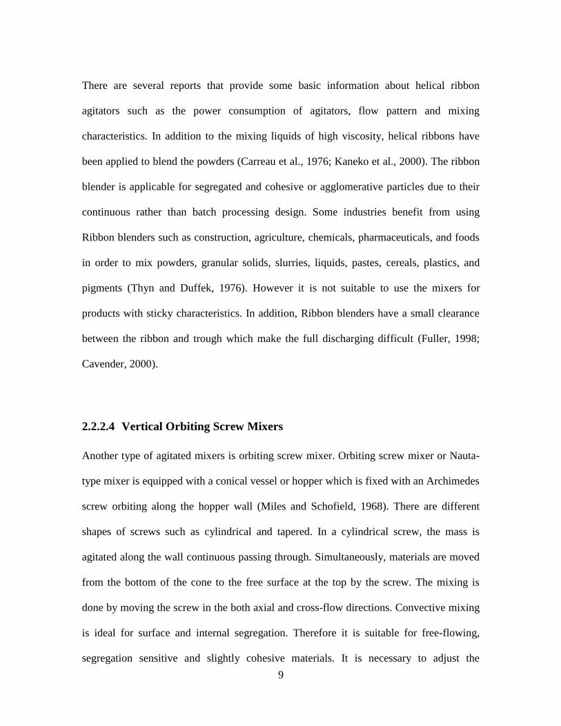
2.2.2.4 Vertical Orbiting Screw Mixers

Another type of agitated mixers is orbiting screw mixer. Orbiting screw mixer or Nauta-

type mixer is equipped with a conical vessel or hopper which is fixed with an Archimedes

screw orbiting along the hopper wall (Miles and Schofield, 1968). There are different

shapes of screws such as cylindrical and tapered. In a cylindrical screw, the mass is

agitated along the wall continuous passing through. Simultaneously, materials are moved

from the bottom of the cone to the free surface at the top by the screw. The mixing is

done by moving the screw in the both axial and cross-flow directions. Convective mixing

is ideal for surface and internal segregation. Therefore it is suitable for free-flowing,

segregation sensitive and slightly cohesive materials. It is necessary to adjust the

10

clearance about six times the average particle diameter to prevent excessive crushing

between the wall and screw blade tip products. While it would be simple to empty the

content and can be adjusted for cooling and heating, cleaning would be hard when it

comes to sticky solids (Hixon and Ruschmann, 1992; Micron, 1998).

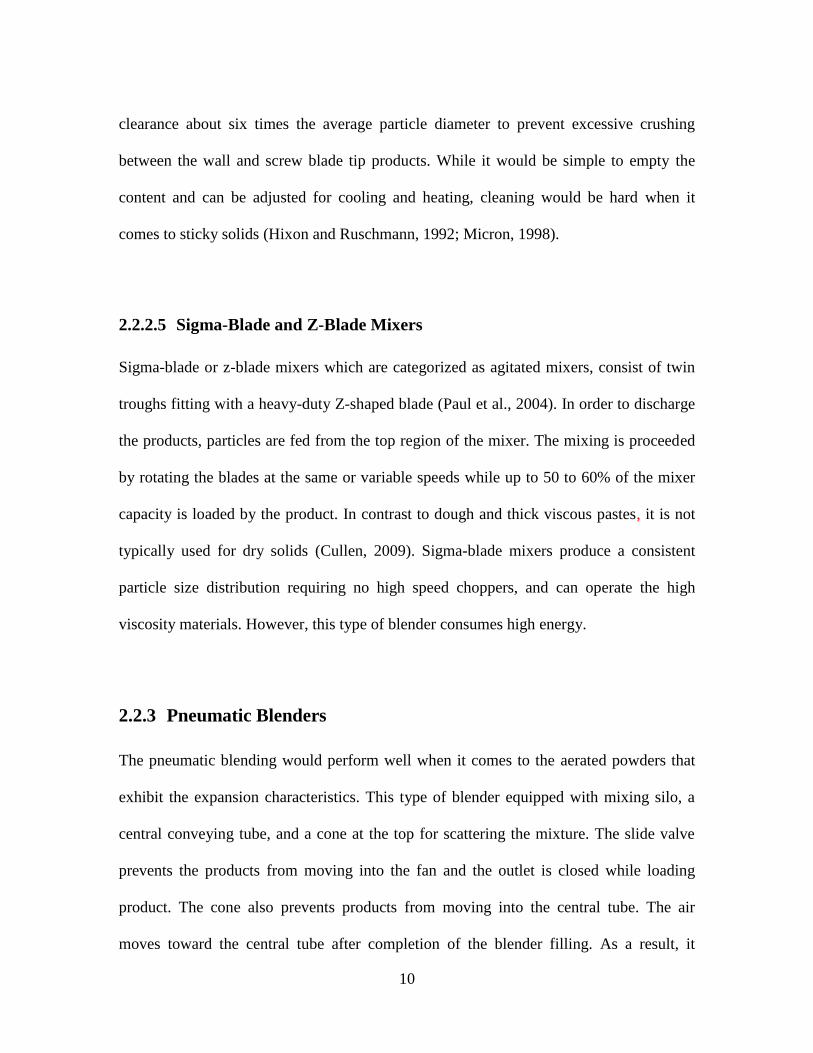
2.2.2.5 Sigma-Blade and Z-Blade Mixers

Sigma-blade or z-blade mixers which are categorized as agitated mixers, consist of twin

troughs fitting with a heavy-duty Z-shaped blade (Paul et al., 2004). In order to discharge

the products, particles are fed from the top region of the mixer. The mixing is proceeded

by rotating the blades at the same or variable speeds while up to 50 to 60% of the mixer

capacity is loaded by the product. In contrast to dough and thick viscous pastes, it is not

typically used for dry solids (Cullen, 2009). Sigma-blade mixers produce a consistent

particle size distribution requiring no high speed choppers, and can operate the high

viscosity materials. However, this type of blender consumes high energy.

2.2.3 Pneumatic Blenders

The pneumatic blending would perform well when it comes to the aerated powders that

exhibit the expansion characteristics. This type of blender equipped with mixing silo, a

central conveying tube, and a cone at the top for scattering the mixture. The slide valve

prevents the products from moving into the fan and the outlet is closed while loading

product. The cone also prevents products from moving into the central tube. The air

moves toward the central tube after completion of the blender filling. As a result, it

11

spreads the product at the top while hitting the cone. There is a fixed duration for mixing.

After aerating, some products show expansion characteristics, for this kind of products,

the pneumatic blending is suitable. In addition, cement and pellet blending are the other

applications of the pneumatic blending. This type of blenders is very quick in processing

and has an efficient mixing approach. In addition, it requires low maintenance while

consume high energy (Vandenbergh, 1994).

2.2.4 Gravity Silo Blenders

The bulk solids are kept in silos to enhance the quality variations of the powder caused by

production method as a function of time. Because of huge amount of silo contents,

homogenization has to take place in situ. Fluidization, internal mechanical recirculation,

and external recirculation are the most typical techniques for silo homogenization which

are done with or without a hopper type of static mixing device. Mixing of any individual

layers is essential to earn the homogenized state of powders (Paul et al., 2004).

To do so, the desired flow patterns should be achieved by designing the silo as large as a

half-angel. It should be noted that the discharge capacity of the central tube has to be

larger than the combined inlet capacity of the port. In addition, harshly similar amounts of

powder should be allowed to enter to the central tube. The gravity blenders are designed

in several ways to allow gravity to cause the mixing of free-flowing materials. This

blender consumes low energy and benefits from simple fabrication and design. In

addition, it is suitable for all free flowing and powdery materials as well as granules.

Gravity silo blenders are quick and economic. However, a large space is needed for

placing this type of blender (Paul et al., 2004).

12

2.2.5 High Intensity Mixers

The impaction mixer is a kind of high intensity mixers and is similar to a typical kitchen

food processor. These mixers are easy to be cleaned and maintained because of their

special shape. Moreover, they are expensive and designed only for specific purposes.

Compare to the similar mixers, these mixers consume more power since the speed of the

blades are around 2000 to 3000 rpm (Miles and schofield, 1968). The impaction mixer,

which is applied as a mixer-granulator, is suitable for adding liquids and/or dry trace

elements (Harnby, 1992). The Henschel mixer is a type of impaction mixer. Intensive pan

mixer and Pan mixers-granulator are two typical models of the high intensity mixers. An

impaction mixer has no dead zone and fast mixing process. With blades moving at high

angular velocities, a pan mixer is intensive type and is applied to cohesive materials. But

it rarely exists in the market and each one is designed for a particular application. These

mixers are divided into batch and continuous types (Vandenbergh, 1994).

2.2.6 High-Shear Mixers

In high-shear mixers, the main impeller blade rotates at relatively high speed. Convective

high shear mixers are suitable for the mixing of the cohesive particles. They are equipped

with especial mixing elements which create high shear stresses in particles. These high

shears are applied to break up cohesive agglomerates. Thus, the individual particles are

liberated to mix with other particles (Cullen, 2009). Any agglomerate is pulverized when

two pressurized rolls press the powder. Before the product is conditioned, the convective

high shear mixers are typically preceded by a convective tumbler mixer to provide a

13

reasonable quality. By using high shearing and simultaneously, by folding and turning the

mixture over in each turn, the material is ground into a very finely divided and well-

mixed consistency by the roller. As a result, the ingredients are mixed intimately

(Nakamura et al., 2009).

High shear blenders are suitable for finely ground powders which are used in the

pharmaceutical industry for the preparation of suspensions and granular products, the

paper manufacturing industry for bleaching and the preparation of paper pulp, the food

industry for food preparation and emulsions for sauces and dressings. In addition, it is

used for emulsification, homogenization, particle size reduction and dispersion. In these

mixers it is possible to add moisture and benefiting from satisfying sensitivity to different

sizes of particles. However, as mentioned, it is not easy to clean and empty these types

of mixers (Harnby et al., 1992; Weidenbaum, 1973).

2.3 Different State of Solids Mixture

A real mixture, unfortunately, shows at least some degree of heterogeneity due to the

incomplete mixing, agglomeration, and segregation, resulting in different types of

textures. Basically, there are three different states of solid mixing which are referred as

perfect, random, and ordered mixing (Muzzio et al., 2003). In some processes such as

chemical reaction, crystallization, and die filling, the quality of the final product depends

on mixing processes and the product is assumed to be homogeneous. A homogenous

mixture assumed that particles are distributed in a state of perfect homogeneity. In other

words, in a homogenous mixture particles alternate themselves along a lattice essentially

14

and have the same composition. Figure 2.1(a) shows the perfect distribution of individual

particles. According to the figure, any sample randomly taken from the mixture will have

the same proportion of each species as the proportions present in the mixture taken as a

whole (Cullen, 2009). A random or stochastic mixture is a mixture in which non-

interacting components such as free-flowing pellets with similar properties (size, shape,

elasticity, etc.) are mixed in an ideal mixer. In a random mixture, particles are freely

moving by a property that does not influence their movement in any way. Also, the

probability of a particle belonging to a certain moiety is statistically independent of the

nature of its neighbors. Considering the definition of a random mixture, it is obvious that

a random mixture cannot be achieved in the presence of significant inter particle forces

such as Van Der-Waals, electrostatic, and cohesive (Muzzio et al., 2003). Figure 2.1(b)

shows the random distribution of individual particles.

Once particles apply surface forces to each other, the formation of agglomeration can be

observed. This system is referred to a cohesive system. Depending on the relative forces

magnitudes between like-particles and unlike-particles, the agglomeration of a single

species (the “guest”) or/and the agglomerates where a small size moiety coats a larger

moiety (the “host”) can be observed. This latter situation is referred to an “ordered

mixture”. Figure 2.1(c) shows the ideal ordered distribution of individual particles. This

figure illustrates that the ideal ordered mixtures have higher degree of homogeneity than

random mixtures (Hersey, 1975). When the ordered units contain different number of

adherent species and the carrier species are randomly mixed, the mixture is called a

pseudorandom mixture. The carrier particles are not saturated with the minor component,

and there are no agglomerates in the mixture. Pseudorandom mixtures present the degree

15

of homogeneity but not the fully disordered texture of the random mixtures (Paul et al.,

2004). Figure 2.1(e) illustrates the pseudorandom distribution of individual particles. The

most troublesome mixtures are textured mixtures which show the segregation texture.

These mixtures complicate the description of particles distribution and characterization.

Moreover, they appeared when the properties of one or more particles cause them to

separate into specific location of the mixture depending on the type of agitation used for

the whole mixture. In general, more free-flowing mixtures show more extreme segregated

states. The cohesive property prevents the segregation of mixture because individual

particles have difficulty in moving independently in the bulk mixture. To determine the

quality of textured mixtures the size, location, and severity of the segregated regions have

to be determined (Muzzio et al., 2003). Figure 2.1(f) illustrates the distribution of

different size of free flowing particles.

16

Figure 2.1. Distributions of individual particles that form a) perfect mixture, b) random

mixture, c) ideal ordered mixture, d) ordered mixture, e) pseudorandom mixture, and f)

textured mixtures.

17

2.4 Quantification of Solids Mixing

Determination and evaluation of the solid mixtures homogeneity and mixing time in the

mixing volume are based on statistical or image analyses. For statistical analysis,

applying a proper sampling technique and sufficient number of samples must be taken.

This technique subjects to relatively complex analyses. In image analysis method, the

mixing efficiency is obtained by digital imaging of the surface rather than by sampling

(Daumann and Nirschl, 2008). Several aspects of the problems associated with solid

mixtures homogeneity and mixing time have been dealt and discussed within the

literature and for different types of blender (Hogg and Fuersten.Dw, 1972; Khakhar et al.,

1999; Wightman and Muzzio, 1998). Various statistical analyses such as estimation of

intensity of segregation, relative standard deviation (RSD), mixture variance, nearest-

neighbors method, Lacey’s method, average-height method, and neighbor-distance

method have been developed to assess the quality of solids mixing in many different

industrial processes (Daumann and Nirschl, 2008). In the following section, these

methods are elaborated.

2.4.1 Statistical Analysis

2.4.1.1 Intensity of Segregation

Paul et al. (2004) illustrated the intensity of segregation is one of the most useful

measures to quantify a solid mixture. The intensity of segregation is a normalized

variance of concentration measurement with the presumption of Gaussian mixing

18

distribution. This raises two problems: (1) the granular mixing may not tend toward a

Gaussian state, and (2) in many practical applications a Gaussian is not the desired

results. Also, the expectation of a Gaussian distribution can cause manufacturers to take

as few samples as possible because a larger number of samples raise the probability of

detecting failed product. Fortunately, granular flows scatter particles more uniformly than

a simple Gaussian distribution. Thus, the intensity of segregation, , is defined as:

(2.1)

where is variance of sampled data, is variance of the same number of randomly

chosen concentration data, and is variance of an initial, typically fully segregated state,

consisting of the same number of data points. In the above equation, the intensity of

segregation is normalized so that = 1 and = 0 correspond to completely segregated and

randomly mixed states respectively.

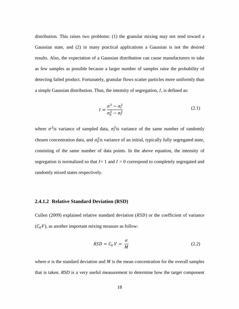
2.4.1.2 Relative Standard Deviation (RSD)

Cullen (2009) explained relative standard deviation ( ) or the coefficient of variance

( ), as another important mixing measure as follow:

(2.2)

where is the standard deviation and is the mean concentration for the overall samples

that is taken. RSD is a very useful measurement to determine how the target component

19

concentration affects mixture quality. RSD calculation is used in pharmaceutical industry

where the active ingredient makes a small proportion of the mixture.

2.4.1.3 Mixture Variance

Mixture variance, , indicates the homogeneity of a mixture and shows the extent to

which individual components of the solids mixture deviate from the required value

(Daumann and Nirschl, 2008). The advantage of variance measurements is its additive

characteristic. In other words, the total variance can be the summation of mixture

variance, sampling error, assay error, and so on. Therefore, mixture variance can provide

detailed analysis of the bed variability by separating the total variance measurement into

the separate dependent measurements. For example, for mixtures of cohesive and free-

flowing components, it is extremely useful that multiple samples are taken from each of a

series of predetermined sampling area and distinguish variability within-location and

between-location. For the tumbling blenders, it is very beneficial to divide the measured

variance into axial variance and radial variance components. Axial variance determines

the concentrations variations between sampling locations, while radial variance estimates

variance within the bed at a single location. For these measurements, the use of a core

sampler can be helpful since the concentration data from a single core and average values

between different cores can be used separately. Formally, for each core j:

∑

(2.3)

20

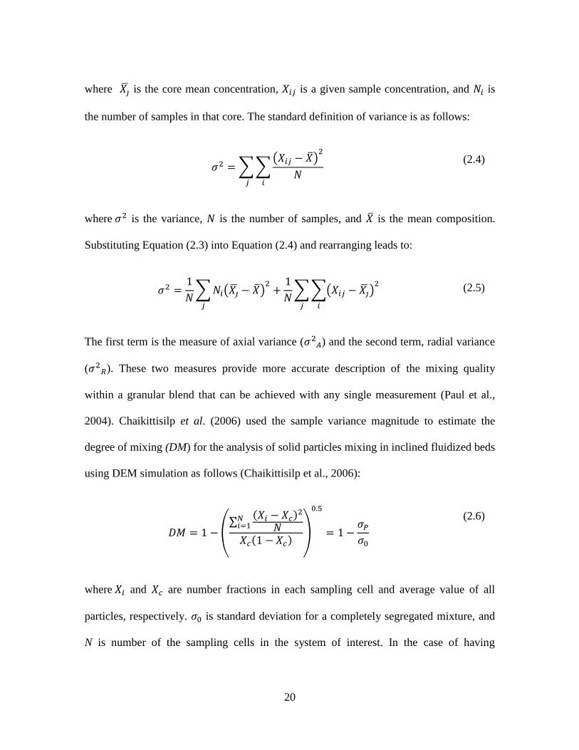
where is the core mean concentration, is a given sample concentration, and is

the number of samples in that core. The standard definition of variance is as follows:

∑∑( )

(2.4)

where is the variance, is the number of samples, and is the mean composition.

Substituting Equation (2.3) into Equation (2.4) and rearranging leads to:

∑ ( )

∑∑( )

(2.5)

The first term is the measure of axial variance ( ) and the second term, radial variance

( ). These two measures provide more accurate description of the mixing quality

within a granular blend that can be achieved with any single measurement (Paul et al.,

2004). Chaikittisilp et al. (2006) used the sample variance magnitude to estimate the

degree of mixing (DM) for the analysis of solid particles mixing in inclined fluidized beds

using DEM simulation as follows (Chaikittisilp et al., 2006):

(∑

( )

( ))

(2.6)

where and are number fractions in each sampling cell and average value of all

particles, respectively. is standard deviation for a completely segregated mixture, and

N is number of the sampling cells in the system of interest. In the case of having

21

completely segregated mixing, DM is equal to zero. Also, once DM is equal to unity, the

mixture is fully random.

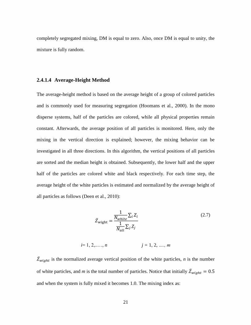
2.4.1.4 Average-Height Method

The average-height method is based on the average height of a group of colored particles

and is commonly used for measuring segregation (Hoomans et al., 2000). In the mono

disperse systems, half of the particles are colored, while all physical properties remain

constant. Afterwards, the average position of all particles is monitored. Here, only the

mixing in the vertical direction is explained; however, the mixing behavior can be

investigated in all three directions. In this algorithm, the vertical positions of all particles

are sorted and the median height is obtained. Subsequently, the lower half and the upper

half of the particles are colored white and black respectively. For each time step, the

average height of the white particles is estimated and normalized by the average height of

all particles as follows (Deen et al., 2010):

∑

∑

(2.7)

i= 1, 2,..…, n j = 1, 2, …., m

is the normalized average vertical position of the white particles, n is the number

of white particles, and m is the total number of particles. Notice that initially

and when the system is fully mixed it becomes 1.0. The mixing index as:

22

( )

(2.8)

This equation means that for , the components of mixture system are fully

separated and for , the bed is fully mixed. The average-height method for analyzing

particle mixing can evaluate the mixing behavior in a fluidized bed. This method is very

useful for visual monitoring of the mixing behavior; however there is a restricted number

of diversity of the particles.

2.4.1.5 Nearest-Neighbors Method

In this method, the vicinity of individual particles is evaluated. The nearest-neighbor

approach is grid independent. Similar to the average-height method, initially, one-half of

the particles are colored black. For each particle, the 12 nearest-neighbor particles are

determined. The system is unmixed if these particles have the same color as the particles

under investigation, whereas the system is fully mixed if one-half of the nearest particle

neighbors have different color. Mixing index is defined as follows (Deen et al., 2010):

∑

(2.9)

is the number of closest neighbors colored differently and is the number of

nearest neighbors. To determine a mixing index, it is important to know only whether a

particle has color 1 or 2, and it restricts this method in quantifying the mixing behavior.

23

2.4.1.6 Lacey’s Method

The Lacey index is based on statistical analysis and was developed by Lacey (1954). For

the calculation of black particles in each cell the variance is defined as follows

(Cullen, 2009; Daumann and Nirschl, 2008):

∑ ( )

(2.10)

is number of samples, is composition of the component in the sample and is the

mean composition or the composition of the component in the whole mixture which is

usually a known value. The better mixture quality is achieved if sample variance or

standard deviation ( ) is lower. Cullen (2009) explained that the sample variance may

include variance from the mixture, the sampling procedure and analytical techniques.

(2.11)

For a binary mixture the upper limit of variance (completely segregated) is given as

follows:

( )

(2.12)

and the lower limit of variance (randomly mixed) is given as follow:

( )

(2.13)

24

where is a fraction of the component in the mixture and is the number of particles in

each sample (Cullen, 2009; Daumann and Nirschl, 2008) . As a result, mixing quality is

estimated as follows (Lacey, 1954):

(2.14)

Basically, the Lacey mixing index is the ratio of mixing achieved to the possible mixing.

Unlike the intensity of segregation, a Lacey index of zero would represent complete

segregation and a value of unity represents a completely random mixture. Finally, the

Pool mixing index is defined as follows:

(2.15)

A pool index of 1 represents a random mixture. To determine a mixing index, it is

important to know only whether a particle has color 1 or 2, and it restricts this method in

quantifying mixing behavior.

2.4.1.7 Neighbor-Distance Method

One of the other methods used to quantify the mixing quality is neighbor-distance method

which is based on the distance between the initial neighbors. At a certain time, the nearest

neighbor is detected for each particle and a pair is made from each particle and its nearest

neighbor.

25

Then, the center to- center distance of the pair is monitored as time progresses. At the

beginning, the distance is on the order of one particle diameter. In the case of having a

fully mixed bed, the center to- center distance can increase up to the bed dimensions. The

mixing index is thus expressed by the equation (Deen et al., 2010):

∑

∑

(2.16)

where is the distance between particle i and its initially nearest neighbor ; is the

distance between particle i and a randomly selected particle k; is particle diameter; and

N is the number of particles. The method just described can be used to calculate the

mixing index for each direction. In this case, the initial distance between the partners in

one direction can be less than a particle diameter. Therefore, the mixing index in the

vertical direction for the neighbor distance method is defined as:

∑

∑

(2.17)

The mixing index for the horizontal direction x or y can be obtained by replacing

subscript z by x or y, respectively. Where, is the average distance in one direction for

two touching particles and is calculated as follow:

(2.18)

26

The neighbor-distance method is the only method in which the mixing index does not

depend on coloring, which makes it the method of choice to quantify solids mixing.

2.4.2 Image Analysis

Image analysis is a novel method and recommended by (Daumann and Nirschl, 2008). In

this method, the optimum mixing time is rapidly determined without sampling and

sample analysis. In fact, the image is analyzed according to the different colors and size

of the particles.

The method of image analysis can be applied to describe the mixing efficiency and obtain

the optimum point of stationary equilibrium. After reaching to the equilibrium, no further

improvement of the mixing quality is achieved by the mixing tool. This method describes

mixing behavior of solids in a short time and without time-consuming sampling and

sample analysis. The segregation on the surface, caused by the different particle sizes,

avoids this method to represent the mixing behavior of the whole mixture. But this

method can be applied to mark one component to investigate the mixing behavior. In this

method, each individual digital image is a copy of a certain mixing state in the mixing

volume at a certain time. The preprocessing and image analysis are done by Photoshop

and image analyzer software respectively. The separated digital images from the

Photoshop are colored black, orange and white. Image analyzer software only detects the

black or white color to analyze any individual pixels. Thus, it transforms the different

particle fractions into a binary image (black or white) for the pixels analysis. From the

counted pixels, the total surface area of the individual particle fractions is obtained and

27

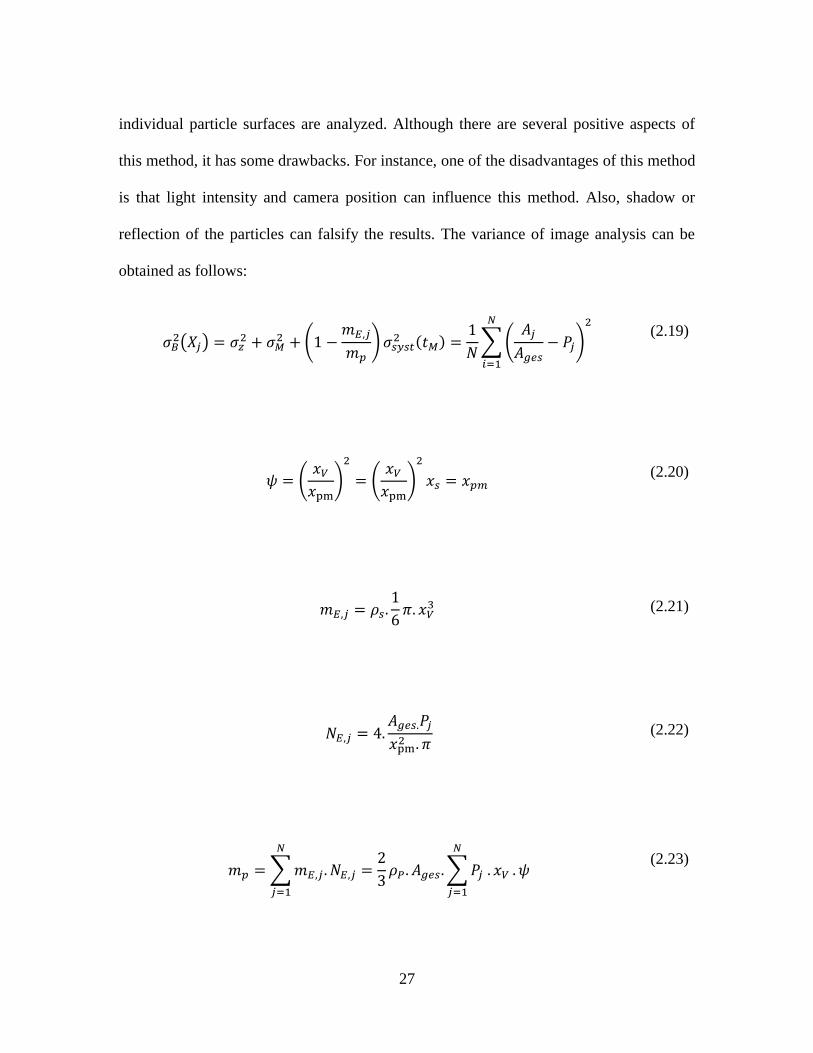
individual particle surfaces are analyzed. Although there are several positive aspects of

this method, it has some drawbacks. For instance, one of the disadvantages of this method

is that light intensity and camera position can influence this method. Also, shadow or

reflection of the particles can falsify the results. The variance of image analysis can be

obtained as follows:

( )

(

)

( )

∑(

)

(2.19)

(

)

(

)

(2.20)

(2.21)

(2.22)

∑

∑

(2.23)

28

where, is variance of image analysis;

presents variance of random mixture;

shows variance of measurement value; denotes systematic variance; is mass of

the individual grain; presents sample mass; shows mixing time; indicates

number of samples; is surface area of the mixing volume , presents the whole

surface area of mixer; denotes target concentration for fraction j; shows solid

density; is equal volume diameter; presents number of individual particles; is

mean projected diameter; is particle density.

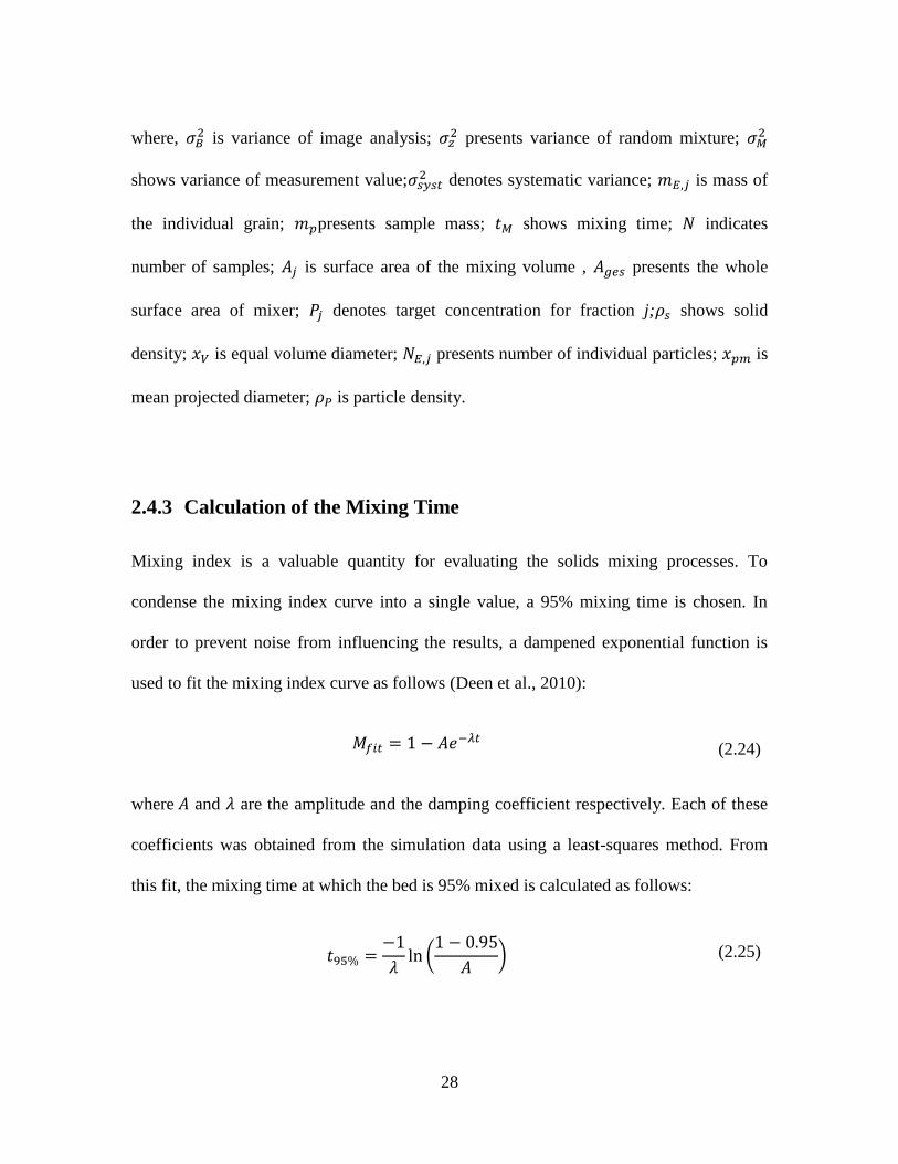
2.4.3 Calculation of the Mixing Time

Mixing index is a valuable quantity for evaluating the solids mixing processes. To

condense the mixing index curve into a single value, a 95% mixing time is chosen. In

order to prevent noise from influencing the results, a dampened exponential function is

used to fit the mixing index curve as follows (Deen et al., 2010):

(2.24)

where and are the amplitude and the damping coefficient respectively. Each of these

coefficients was obtained from the simulation data using a least-squares method. From

this fit, the mixing time at which the bed is 95% mixed is calculated as follows:

(

)

(2.25)

29

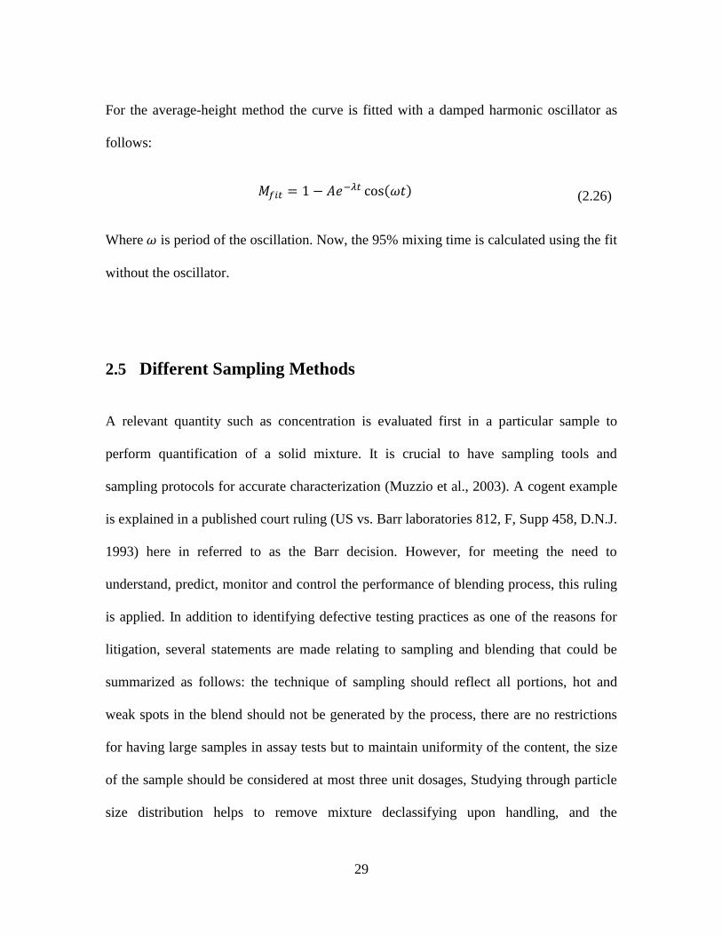
For the average-height method the curve is fitted with a damped harmonic oscillator as

follows:

( )

(2.26)

Where is period of the oscillation. Now, the 95% mixing time is calculated using the fit

without the oscillator.

2.5 Different Sampling Methods

A relevant quantity such as concentration is evaluated first in a particular sample to

perform quantification of a solid mixture. It is crucial to have sampling tools and

sampling protocols for accurate characterization (Muzzio et al., 2003). A cogent example

is explained in a published court ruling (US vs. Barr laboratories 812, F, Supp 458, D.N.J.

1993) here in referred to as the Barr decision. However, for meeting the need to

understand, predict, monitor and control the performance of blending process, this ruling

is applied. In addition to identifying defective testing practices as one of the reasons for

litigation, several statements are made relating to sampling and blending that could be

summarized as follows: the technique of sampling should reflect all portions, hot and

weak spots in the blend should not be generated by the process, there are no restrictions

for having large samples in assay tests but to maintain uniformity of the content, the size

of the sample should be considered at most three unit dosages, Studying through particle

size distribution helps to remove mixture declassifying upon handling, and the

30

prospective validation program must involve a time of the mixing study (Muzzio et al.,

1997).

There is no offered procedure helping to achieve the goals in the mentioned statements.

There are also some unclear points in the Barr decision. Firstly, it is not explained how to

achieve uniformity, and no information about the number of samples and the location of

them in order to achieve representatives. Secondly, hot and weak spots are not identified

and there is no description on finding them and preventing them from forming. Also, a

couple of issues are omitted. The first one is sampling errors and the other one is

segregation. A thief probe is applied to obtain samples. Using such sampling devices like

thief probe may generate large errors in composition of the sample through and this is not

included in the Barr decision statements. The second issue is segregation, which is proved

in practice that departing is unavoidable while handling with powder mixtures. This,

however, is covered by referring it to through particle size distribution. This solution is

not easy to follow due to the current technology and may result in the complications in

other performance objectives e.g. dissolution. It also requires particular size values

(Muzzio et al., 1997). Physical and non-invasive methods are two methods of sampling

(Paul et al., 2004).

2.5.1 Physical Sampling Methods

The most important barrier in the way of characterizing granular mixtures is the absence

of a correct and reliable data for the performance of powder mixers. In order to analyze

the powder mixture, analyzing samples from the bulk mixture to review their

characteristics is needed (Muzzio et al., 2003). It is undeniable that, the sample cannot be

31

taken from a flowing stream. Instead, the sample should be taken from a static bed.

Thieves, as typical sampling tools for powder, take samples from the interior regions

while is inserted into the bed. All the regions of the bed should be included in sampling.

If not, unexpected segregation may happen in the granular mixture. Missing regions of

poor mixing is unavoidable if sampling is limited to few locations. Additionally, the

results may change due to disturbance of a mixture caused by sampling of a powder

mixture (Paul et al., 2004). Multiple assumptions relating to the powder mixture are

needed for the sampling techniques. Granular materials are likely to mix slowly and also

are expected to experience segregation in the mixture, where random distribution is

considered for sampling process by many engineers. However, this may result in false

conclusion since there are few positions that sampling would characterize the mixture.

Therefore, it would be unwise to assume the thief sampler identifies the true composition

of the mixture and it has to be taken note of during the developing and evaluating

sampling and characterization techniques (Muzzio et al., 1997). There are several articles

(Berman and Planchard, 1995; Berman et al., 1996; Muzzio et al., 1997; Poole et al.,

1965) regarding the sampling method. Thief sampling has two types of behaving, which

are the side sampling thief and end sampling thief; where both are reviewed here (Paul et

al., 2004).

2.5.1.1 Side Sampling Thief

A tube with a slot in its side forms the side sampling. To do the sampling, particles flow

into a cavity as the slide is opened. Then after the slide is closed, the extraction of the

inserted sample begins. However, using this type of sampling has its own shortages.

32

Particles in the insertion rout will be rearranged. Moreover, Samples that extracted using

this technique will consist smaller than the product because the small particles are easy to

flow (Muzzio et al., 1997; Venables and Wells, 2002). When the probe break the powder

bed, different powder species flow into the probe making the thief probe show large

errors when characterizing a mixture. This is the most important barrier on using slide

sampling thief. This problem has been selected for studying by some researchers (Berman

and Planchard, 1995; Berman et al., 1996; Gopinath and Vedaraman, 1982; Muzzio et al.,

1997). Where, two typical pharmaceutical materials with different sizes were used for

sampling by Berman, et al. (1996) to investigate the performance of two kinds of side-

sampling thieves. On the other hand Muzzio, et al. (1997) considered comparing three

unmixed granular small glass beads beds. These sample materials use Globe- Pharma and

the groove thief which cause bed distribution.

2.5.1.1.1 Globe-Pharma Probe

Globe-Pharma probe is a kind of side sampling tool. This sampler is made of a hollow

sleeve with some openings around a rotating interior pipe and several cavities that can be

lined up with the exterior pipe opening. Only the lower cavity is used and the upper one

will be filled by a solid die. Opening and closing the sampling is done by rotating the

inner pipe. The thief is penetrated into a selected depth while cavities are sealed. Cavities

are filled with powder when the interior piped rotates. Then the thief is removed from the

bed. This device is limited to few sampling at a certain time (Muzzio et al., 2003; Muzzio

et al., 1997)

33

2.5.1.1.2 Groove Thief

An exterior hollow sleeve with an opening running the length of the pipe and surrounds a

rotating interior pipe form this sampling tool. Like Globe-Pharma probe, the interior pipe

is applied to do the opening and closing of the cavity. Subsequently, it is inserted to the

powder bed and a vertical core of powder is captured using rotation of the interior pipe.

After that the core will be divided into smaller samples by the means of a special device.

As the thief opens, a number of small trays are filled by materials. This device makes it

possible to have many samples with identical size at the same time (Muzzio et al., 2003).

2.5.1.2 End Sampling Thief

In the end sampling tool, which consists of a tube with an aperture at the distal end, first

the tube is inserted in the bed. After aperture is opened, the probe inserted deeper in order

to rake the sample. Eventually, by closing the aperture the sample will be extracted. Like

side sampling methods, end sampling does not passively flow the particles into the cavity.

Instead, they force the particles. So, this caused problems in particles flow ability. Also,

accuracy is very important in this technique, since the thieves are bulky and disturb the

material while inserting (Muzzio et al., 1997). In the following, two different end

sampling thieves, which are end-cup sampler and core sampler, are elaborated.

2.5.1.2.1 End-Cup Sampler

A couple of thin rods, one carrying a cup at the end and the other one is attached to a

rotating cap aligned with the top of the cup, form this sampling tool. In order to decrease

34

the rearrangement of the powder bed during the insertion, the cup is tapered to a cone.

The sampling is completed by inserting the sampler into the powder bed along with a

sealed cap. To release powder to the cup, cap must be rotated and after the closing of the

cup, the thief is removed from the bed. It should be considered that only one sample can

be taken at a time (Muzzio et al., 2003).

2.5.1.2.2 Core Sampler

Core sampler, another kind of end sampling tools, consists of a thin-walled tube with a

mechanized extrusion apparatus. This sampler can takes an entire neighboring core of

particles throughout the depth of insertion. The thin-walled tube is inserted into the bed

and the extrusion apparatus permits samples to be extracted. This device is equipped with

end cap which get opened during insertion and closed during extraction. In this technique,

the core extends through the depth of the sampling tube and causes precise determination

of concentrations between different layers of the bed. Also, the size of sample is

completely variable and can easily be regulated for different mixtures (Muzzio et al.,

2003).

2.5.2 Non-Invasive Methods

In contrast to the physical sampling technique, the non-invasive methods do not only cost

too much but they are very complicated methods. However, they provide a lot of

information regarding the quality of the mixture. The different types of these methods are

the diffusing wave spectroscopy, positron emission tomography, magnetic resonance

35

imaging, and X-ray tomography. In the diffusing wave spectroscopy, configuration

concludes the measurement of statistics of fluctuations. During the mixing process, the

positron emission tomography that used an array of external photomultipliers, a single

radioactive particle is tracked. In X-ray tomography, a group of radio particles are tracked

in a flow of interest. In magnetic resonance imaging, a configurations structure that

consists of magnetic moments of hydrogenated particles is tracked for a short time(Paul et

al., 2004). Uncertain sources of error exist for the solid mixing data analysis like

sampling technique and analytical method. The location, size, number, and selection of

samples should be considered in order to minimize the errors. The sample should be

captured from several locations of the mixer considering what the goal of the study is

about. Selecting a suitable location for sampling would determine of flow patterns that

would come in handy. It should be noticed that the sample has to be captured at the

discharge spout to estimate the performance of the mixer. In addition, to avoid

segregation of the sample, it should be cared during the process with capturing the

samples from a moving stream). In addition, instead of taking the sample from a part of

the stream, it should be captured in a short amount of time from the whole stream (Paul et

al., 2004). To obtain the best result, sample size should be the same as the amount of the

material at which homogeneity is desired. Sample variance in random mixture is identical

to the sample size. In other word, if small samples are taken, more samples are needed to

decrease the determination error. Sample size can be reduced by using techniques such as

spinning riffler, chute riffler, and ICI method (Allen and Tildesley, 1987; Allen, 1981).

In batch processes, the mixer is stopped and sampling begins from several locations of the

bed. Since there is no mixture mean or standard deviation available, priori or historical

36

data is applied as guideline. In continuous processes, sampling is done at the mixer outlet

according to the rules of sampling. Depending on the capability of the analytical

technique, the number of taken samples is different (Allen, 1981). When it comes to the

small stationary bed condition or pile, sampling will be proceeded by chute riffler or

spinning riffler. Pneumatic lance or a scoop is required when it is about a large stationary

bed. Online samplers such as whole stream samplers, cross-cut samplers, and split-stream

samplers are also exist. But to choose the suitable option, some properties should be

considered. For instance, flow-ability and friability of the material, particle size, desired

sample size, and availability of space are some of these parameters. Also, sampler should

be capable of collecting maximum size of particles, fitting into the space and not have

limitation on size of the sample. Moreover, the sampler has to be flow-able when moving

to the mixture (Paul et al., 2004).

2.6 Discrete Element Method

Processing of particulate materials has a significant effect on the production cost in many

industries. However, these costs can be minimized by increasing processing through-put,

production efficiency, and decreasing the product waste. Thus, the innovative designs and

operational techniques are required. A huge amount of savings may be gained by any

small percentage improvement in the performance. Discrete Element Modeling (DEM) is

such a tool for modeling particulate flows and processes.

DEM technology is essentially a numerical technique to model the movement of the

particles interacting with each other through collisions (Tijskens et al., 2003). DEM

37

technology was originally pioneered by Cundall and Strack (1979) to simulate granular

flow. Then, it was applied to different simulation models in many fields such as granular

mixing(Asmar et al., 2002; Cleary, 1998; Rhodes et al., 2001) and dragline excavation

(Cleary, 1998); ball mill operation (Mishra and Rajamani, 1992); silo filling (Holst et al.,

1999). DEM simulating of a particulate process causes to achieve an accurate

representation of the bulk behavior of the material and is done by defining material

properties that affect the bulk behavior. In the case of having small size of particles,

relative to the volume of bulk material further assumptions and scaling are required to

make the problem computationally tractable.

In fact, to model the behavior of particles in a mixing vessel, DEM simulates every

particle dynamic individually. Then it numerically integrates their accelerations which are

the consequences of all forces, including contact force and gravity force. Every time step

starts with the recording of particle positions and evaluation of the particle interactions.

Then, all forces acting on each particle are calculated and Newton’s second law is applied

to determine the accelerations. Afterwards, the accelerations are integrated with time to

find the velocity and position of each particle in the new state. This process is repeated

until the end of simulation (Lu and Hsiau, 2008). Physically, particles in a DEM problem

are assumed as rigid bodies and the contacts between them as point contacts. In reality,

the majority of particles are definitely more or less deformable. In computational model,

this property is approximated by allowing particles to overlap and is referred as virtual

overlap, δx .The forces which result from a contact between two particles are related to

their virtual overlap by a contact force model (Cleary and Sawley, 2002). Most of the

DEM articles consider spherical elements (3-D) or disks (2-D) element because can

38

define the geometry of particle by a single value which is radius. By this consideration

for the shape only one type of contact between particles is considerable.

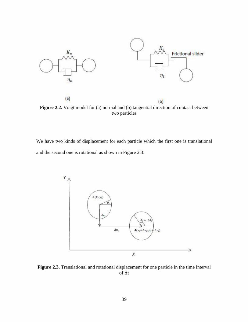
The first issue for using DEM process is finding the contact force. Contact force is a

vector. This vector is decomposed into two vectors, a normal vector and a tangential

vector. We can apply the Voigt model for both direction of force which involves the

elastic and damping force. Effect of friction considered as a frictional slider. Figure 2.2

show Voigt contact model of two particles. Equation of Newton’s second law of motion

for this system is:

(2.27)

(2.28)

Subscript of n and t are denoting normal and tangential direction respectively. , ,

, , and are the mass of the particle, the rotation of the particle, the moment of inertia

of the particle, the elastic coefficient of two particles in contact , displacement of the

vector and the damping coefficient of two particles in contact respectively.

39

Figure 2.2. Voigt model for (a) normal and (b) tangential direction of contact between

two particles

We have two kinds of displacement for each particle which the first one is translational

and the second one is rotational as shown in Figure 2.3.

Figure 2.3. Translational and rotational displacement for one particle in the time interval

of

40

Contact of particles in DEM approach is too complicated since each particle has several

contacts in specific times. In this study, we suppose that two particles i and j which are in

contact with each other in a specific time as shown in Figure 2.4.

Figure 2.4. Normal and tangential displacement for two particles in contact.

Acceleration of each particle can be calculated from Newton’s second law and with the

acceleration we can find velocity and displacement of each particle as follows:

( ) ( )

(2.29)

( ) ( )

(2.30)

41

(2.31)

In fact, the results of DEM simulation have to match the results of physical experiments

within an acceptable level of accuracy. To achieve this, the input of material properties

and interaction parameters such as coefficients of friction and shear modulus has to be

known as DEM inputs. Indeed, DEM simulation results are influenced by the particle

inertial properties i.e. size, shape, density, also mechanical properties i.e. stiffness,

elasticity, and plasticity, interaction terms between particles and other objects, and

particles or boundary surfaces. The interaction term depends on the selection of contact

models which may include parameters such as friction, restitution coefficient, cohesion,

fluid drag, electrostatic force, and magnetic force, and so on. The most important

limitation of the DEM discrete element method is the computer performance. The

number, size, and shape of the particles (irregular shapes are very difficult to simulate)

would be the main issue for using DEM.

2.7 Contact Force Models

In the mixing of solid particles, the motion of each individual particle is modeled by

solving Newton’s second law of motion. Forces applying on a particle are composed of

the contact force( ) and gravitational force ( ). Basically, the contact force is

composed of a normal ( ) and a tangential force ( ) as follows (Chaikittisilp et al.,

2006):

42

(2.32)

So far several different models have been developed to model normal and tangential

forces. In the following sections the most common developed models for the normal and

tangential forces are described.

2.7.1 Normal Contact Force Models

Force schemes are characterized into four groups according to the dependency of the

normal force on the overlap and the displacement rate. Four main groups are defined as

continuous potential models, linear viscoelastic models, non-linear viscoelastic models

and hysteretic models (Kruggel-Emden et al., 2007). In the following, the most relevant

models of these classes are briefly discussed.

2.7.1.1 Continuous Potential Contact Models:

Continuous potential contact models are introduced by three approaches that are briefly

described below. These approaches are for granular material only and in the context of

DEM continue potential contact model. In all of these approaches, normal force is

obtained by combining the potential force and dissipative component as shown in the

following equation.

(2.33)

43

where , and

are the total normal force, potential normal force and dissipative

component of normal force respectively. The only difference between these three

approaches is how to define the potential force and the dissipative component. Allen and

Tildesley (1987) and Rapaport (2004) also applied continuous potential models for

Molecular Dynamics (MD) simulations on the atomic or molecular level (Kruggel-Emden

et al., 2007; Rapaport, 2004).All contact force in the category of continuous potential

contact models exhibit one limitation which causes plastic deformation to be inaccurate.

2.7.1.2 Linear Viscoelastic Models (Linear Spring Dashpot)

Linear models are the most common models applied in discrete element simulations. In

these models, the normal force ( ) consists of two parts: one for modeling the elastic

repulsion, referred to as elastic spring, and the other for the viscous dissipation, and is

understood as the displacement rate dependent damper (Kruggel-Emden et al., 2007)

(2.34)

where and are the stiffness of linear spring and a constant of the velocity

proportional amper respectively. Note that this model is not restricted for the linear case,

but is damped for the harmonic oscillator force (Kruggel-Emden et al., 2007). Linear

viscoelastic models (Figure 2.5) were used by Kruggel-Emden et al. (2007) for the DEM

modeling of granular flow in hoppers. Limtrakul et al. (2004) used linear viscoelastic

models for DEM modeling and simulation of a catalytic gas-solid fluidized bed reactor

(Limtrakul et al., 2004).

44

Figure 2.5. Schematic of a viscoelastic model

Linear viscoelastic models are valid for some materials such as bio-particles in a

reversible deformation and nanoparticle fusion in irreversible deformation. Linear

viscoelastic models have been widely used by many researchers.

(

(

(

)

)

)

(2.35)

(

(

)

)

(2.36)

where and are the coefficient of restitution and the duration of collision

respectively. All contact forces in the category of linear viscoelastic models exhibit one

limitation which causes plastic deformation to be inaccurate.

45

2.7.1.3 Nonlinear Viscoelastic Models (Nonlinear Spring Damper)

Before introducing nonlinear viscoelastic models, we should be aware of one important

contact force which is the Hertz (1882) model. Hertz developed a nonlinear model for the

elastic contact. Several contact force models have been developed based on the Hertz

theory. These models extended the original approach of Hertz by limiting the elastic

contacts (Kruggel-Emden et al., 2007).

Most of these models that described here, are modifications of Hertz (1882) model and do

not allow an analytical solution of their differential equations. Hertz (1882) proposed an

equation for the nonlinear elastic model, which is:

(2.37)

and are stiffness of non-linear spring and displacement respectively. All contact

forces in the category of non-linear viscoelastic models have two limitations. The first

limitation is that it is not accurate when the model experiences plastic deformation and

the other is the requirement to have a small time step for the simulation.

2.7.1.4 Hysteretic Models

In the hysteretic models (Figure 2.6), the effect of plasticity is taken into account and the

velocity dependent damping is prevented. All hysteretic models are applied to collision

with permanent deformations. These models can be linear or nonlinear with different

springs and different stiffness for the loading and unloading period.

46

Figure 2.6.Schematic of a hysteretic model

All contact forces in the category of hysteretic models have one limitation which is

requiring a small time step for simulation. As a result, they have computationally

expensive simulations.

2.7.2 Tangential Force

For the tangential direction of force, there is a main approach which was proposed by

Mindlin and Deresiewicz (1953) for elastic material which is described below (Mindlin

and Deresiewicz, 1953).

2.7.2.1 Mindlin and Deresiewicz (1953)

Mindlin and Deresiewicz (1953) proposed the theory of frictional elasticity of a compliant

sphere in contact with a wall for the tangential direction. They developed a set of rules for

the generalization from simple cases to the oblique impact problem with an incremental

47

procedure. They developed models for normal and tangential contact problems once:

tangential displacement is zero and normal displacement varies, normal displacement is

constant and tangential displacement varies, and both normal and tangential

displacements vary.

According to their theory, once the tangential displacement is zero and normal

displacement varies, the normal force displacement is modeled as follows:

(2.38)

√

(2.39)

where , , , , and are nonlinear elastic stiffness, normal force,

displacement rate, equivalent Young’s modulus and reduced radius, respectively.

Also, when normal displacement is constant and tangential displacement varies the

tangential force is modeled as follows:

( )

(2.40)

(

)

(2.41)

48

√

(2.42)

where presents tangential force, shows incremental stiffness, denotes tangential

displacement, is a symbol of initial tangential displacement, presents initial

incremental stiffness, shows equivalent radius, and is total normal displacement.

2.8 DEM Utilized

Mixing of solid particles has a significant role in many fields such as chemical,

agricultural, ceramic, mechanical and civil engineering and pharmacy. All industries

share a common interest that is the characterization of powder behavior. Also, DEM

technology has been used over the past 25 years for simulating mixing processes and the

behavior of granular materials in different industries; so many articles have been

published on the some subjects related to DEM. Several articles were published regarding

flow pattern using DEM, however, only a few articles were found in literature regarding

mixing performance because of the complications inherent mixing method. In the

following section, articles which were discussed regarding mixing performance of the

mixer using DEM method are categorized by mixer type.

2.8.1 Tote Blender

Sudah et al. (2005) worked on simulation and experiments of mixing and segregation in a

tote blender. They applied 3-D DEM to study flow and mixing of spherical, free-flowing

49

particles in a 14L tote blender. They used glass beads for the simulation and experiment

and they used one visco-elastic contact force, namely the Walton and Braun (1986)

model, for the normal and tangential contact forces. For sampling, they used large

transparent core samplers which were suggested by Muzzio et al. (1997). For this study,

they used plastic core sampler tubes (3/4 in. outer diameter, 11/16 in. inner diameter) and

the number of that sampler tubes for this study was nine. They applied mono-disperse and

bi-disperse mixtures in this tote blender. For mono-disperse mixtures, the number of the

particles was 3700 at 40% fill and 5500 at 60% fill. For bi-disperse mixtures, they only

had one simulation at 40% fill consisting of 1833 12mm beads and 14666 6mm beads. All

mono-disperse and bi-disperse simulations were performed at 10 RPM. In this study

mixing and segregation curves were constructed by plotting the relative standard

deviation (RSD) versus the number of blender revolutions (N) or mixing time. Also, they

plotted frequency vs. particle velocity to find the probability density function (pdf) of

axial velocities for a mono-disperse 60% fill level case (Sudah et al., 2005; Walton and

Braun, 1986). One year later, Arratia et al. (2006) studied the mixing and segregation

mechanisms in the tote blender via DEM simulations. They assumed that the granular

material was an idealized mixture of the frictional and nearly inelastic spherical particles,

so each particle may have interaction with its neighbors or with the boundary of the

blender through both normal and tangential forces. They chose the Walton and Braum

model (1986) for the normal force as well as tangential force. They used K1=6000 N/m.

to ensure that the overlaps α1 and α0 remain small compared to the particles sizes. They

choose two types of particle with coefficient of restitution (ε) equivalent to 0.7 and 0.5.

So K2 for these particles were 12200 N/m and 24000 N/m respectively. The particle size

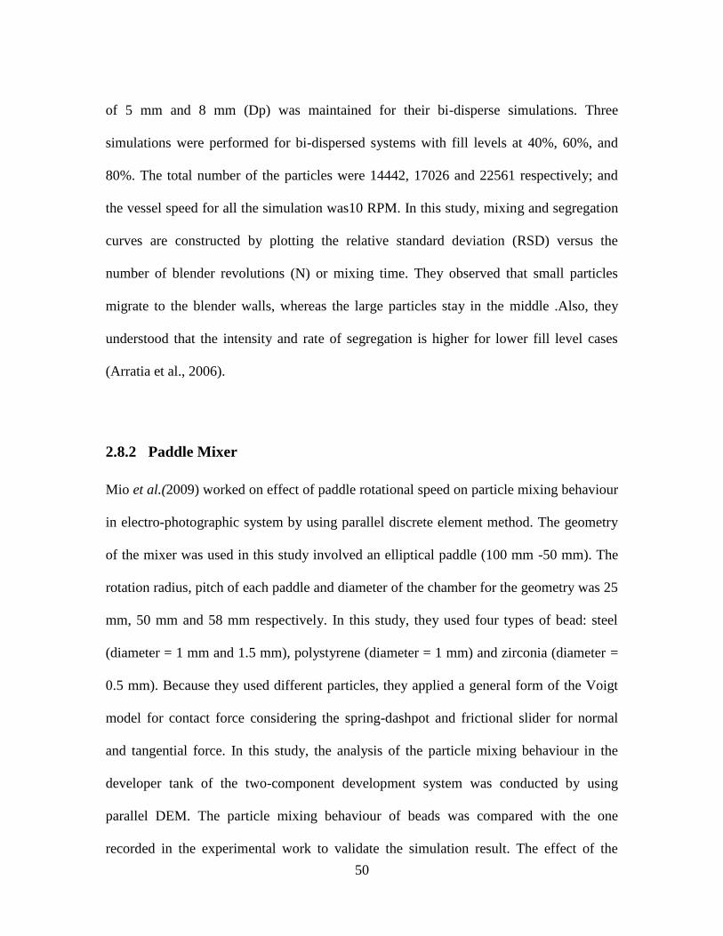
50

of 5 mm and 8 mm (Dp) was maintained for their bi-disperse simulations. Three

simulations were performed for bi-dispersed systems with fill levels at 40%, 60%, and

80%. The total number of the particles were 14442, 17026 and 22561 respectively; and

the vessel speed for all the simulation was10 RPM. In this study, mixing and segregation

curves are constructed by plotting the relative standard deviation (RSD) versus the

number of blender revolutions (N) or mixing time. They observed that small particles

migrate to the blender walls, whereas the large particles stay in the middle .Also, they

understood that the intensity and rate of segregation is higher for lower fill level cases

(Arratia et al., 2006).

2.8.2 Paddle Mixer

Mio et al.(2009) worked on effect of paddle rotational speed on particle mixing behaviour

in electro-photographic system by using parallel discrete element method. The geometry

of the mixer was used in this study involved an elliptical paddle (100 mm -50 mm). The

rotation radius, pitch of each paddle and diameter of the chamber for the geometry was 25

mm, 50 mm and 58 mm respectively. In this study, they used four types of bead: steel

(diameter = 1 mm and 1.5 mm), polystyrene (diameter = 1 mm) and zirconia (diameter =

0.5 mm). Because they used different particles, they applied a general form of the Voigt

model for contact force considering the spring-dashpot and frictional slider for normal

and tangential force. In this study, the analysis of the particle mixing behaviour in the

developer tank of the two-component development system was conducted by using

parallel DEM. The particle mixing behaviour of beads was compared with the one

recorded in the experimental work to validate the simulation result. The effect of the

51

paddle rotational speed on the mixing behaviour of the carrier particle was investigated to

optimize the mixing process in the electro-photographic system. Also, they plotted the

mean radial velocity vs. paddle rotation angle and relative number of contacts between

particles vs. mixing time in each area and compared with the experimental data (Mio et

al., 2009).

2.8.3 V-Blender

Lemieux et al. (2006) studied the investigation of solids mixing in a V-blender using the

discrete element method. They used a 16-qt Patterson–Kelly V-blender as geometry. In

this study, five simulations were performed, both mono-disperse and bi-disperse with 3

mm and 6 mm particles. They had two rotational speeds, 15 and 30 rpm, at a fill level of

45% for their simulations. For the contact force, they used the Cundall and Strack (1979)

model as normal contact force and the Vu-Quoc et al. (2001) contact model for tangential

force, based on the Mindlin and Deresiewicz (1953) contact force). The relation between

the normal and tangential contact force was considered in this study byrefrence to the

method of the Zhou et al. (2002). In this work, the relative standard deviation (RSD) was

found for evaluation of the homogeneity of the mixture as well as time needed to achieve

this homogeneity by DEM concept. They plotted velocity vs. time, torque vs. time and

RSD vs. number of revolutions for each case. To validate this data, they found torque

experimentally and compared with the simulations. Moreover, they worked on a

comparative study of the mixing of particles in a V-blender and a bin-blender. Both

blenders considered in this study are 7.5L. For bi-disperse simulation and experimental

work they used two particles with mean diameters of 491 µm and 510 µm and the number

52

of particles were 420000 and 780000. They performed several experiments and

simulations at rotational speeds of 15, 30 and 45 and at fill level of 35%, 50% and 65%.

Contact force for interaction between particles for this study was the Cundall and Strack

model (1979). Also, for the normal force and tangential force, the correction of Bertrand

et al. (2005) was considered by the authors. They plotted the relative standard deviation

(RSD) vs. number of revolution & mean radial and axial velocity vs. time for both V-

blender and bin-blender in some different simulation and compared them to each other.

With this work they concluded that the performance of the V-blender was significantly

superior to that of the bin-blender for lab-scale blenders (Bertrand et al., 2005; Lemieux

et al., 2008; Lemieux et al., 2007; Vu-Quoc and Zhang, 1999).

2.8.4 Double Cone Blender

Manickam et al. (2010) studied the mixing simulation in a double cone blender and

validated this simulation, experimentally. The geometry for this simulation was 5.6 in.

diameter and 12 in. high, with a 3 in. straight side. They used homogenous system size

(diameter; 3 mm) with two different colours and the number of particles of each colour

was 25000. Their simulation was at the 10%, 20% and 40% fill level of the vessel and

rotational speed of 30 RPM. They investigated the effect of size of particle, effect of fill

and effect of vessel speed with concentration of red particles vs. time in different

circumstances. They used a digital camera to validate their simulation and prediction of

numerical simulation. T= 0, 2 and 5 was the time sequence were captured by the digital

camera (Manickam et al., 2010).

53

2.9 Research Objectives

It is obvious from our comprehensive literature review that the information regarding the

solid mixing is still inadequate. Little information is also available regarding the mixing

performances of the slant cone and ploughshare mixers in the literature. Therefore, the

main objectives of this work are:

To investigate the mixing efficiency of solid particles in a slant cone mixer as a

function of initial loading (side-side, top-bottom, and back-front), drum speed, fill

level, and agitator speed using discrete element method (DEM);

To assess the mixing index as a function of the initial loading, the rotational

speed, fill level, and the particle size for a six-blade ploughshare mixer through

the discrete element method (DEM).

54

3. Using Discrete Element Method to Analyze the Mixing of

the Solid Particles in a Slant Cone Mixer

3.1 Introduction

Undoubtedly, powder blending plays a prominent role in several industries that are

related to particulate processing. Thus, the efficiency and optimization of the powder

mixers are critical issues for food, pharmaceutical, ceramic, metallurgical, and chemical

industries. The industrial powder mixers can be broadly classified into the following

categories (Paul et al., 2004): tumbling mixers, agitated mixers, pneumatic blenders,

gravity silo blenders, high-intensity mixers, and high-intimacy or high-shear mixers.

There are some essential factors that should be considered before any attempt to select a

proper powder blender for a specific application. These vital aspects are the specifications

of the materials to be mixed, process safety, industry regulations, labor availability, single

or multiple operations, the way that the material is transmitted to and from the blender,

and the procedure that the mixer will be integrated into the plant.

Multiple industries are using tumbling blenders widely in granular mixing operations,

including pharmaceutical, cosmetics, mining, food, energy, polymer, and semiconductor.

Tumbling blenders are easy to operate, available in various capacities and are able to

operate with shear sensitive or non-agglomerating materials. Their cleaning and emptying

procedures are easy. Moreover, tumbling blenders are suitable for blending of dry and

free flowing materials (Alexander et al., 2004; Kuo et al., 2005). Finally, the tumbling

55

mixers benefit from simple mixing mechanisms. A closed vessel rotates around the axis

in a tumbling mixer. Mixing in this type of the blender is achieved due to the random

motions of the particles rolling down from an inclined surface. The counter rotating of the

vessel and the installation of the internal baffles would also enhance the mixing of

particles (Cullen, 2009). Of course there are some negative points on using the tumbling

mixers. One of them is the high chance of the segregation of the particles. Furthermore,

mixing is typically confined to the surface of the powder bed and leaving large regions

undisturbed during long periods of the mixing cycle. In addition, tumbling mixers are not

suitable for the agglomerating particles (Cullen, 2009; Poux et al., 1991).

Generally, four principal types of tumbling mixers are utilized for powder blending.

These four popular blenders are V-shape, double cone, tote, and slant cone (Gemco

trademark). Both symmetrical and asymmetrical designs are used in the fabrication of the

tumbling mixers. V-shape, tote and double cone blenders are symmetrical blenders and

their axes of rotation is perpendicular to the line of symmetry. On the other hand, two

commercial asymmetrical blenders in the market are the slant cone blender and the long

leg V-shape design, where one leg is longer than the other. The asymmetrical blenders

superimpose the axial flow of the material in the direction of rotation. In fact, the

materials inside the blender are forced across the vertical axis of the unit each half

revolution. This enhances the mixing quality in a shorter blend time. One advantage of

the slant cone mixers over other asymmetrical mixers is the possibility of installing the

internal agitator with an intensifier bar, which is useful for high intensity blending or

mixtures that may lump.

56

Our comprehensive literature review revealed that little information is available regarding

the mixing performance of the slant cone mixers. Therefore, the main objective of this

study was to analyze the mixing of solid particles in the slant cone mixer through the

discrete element method (DEM), which is a reliable simulation method for assessing the

particulate systems. In this work, DEM was employed to evaluate the mixing efficiency

of the slant cone mixer as a function of the initial loading, drum speed, fill level, internal

agitator speed and rotation mode. To validate the model, the simulation results were

compared to the experimentally measured values.

3.2 Specifications of the Mixer and Experimental Methods

In the present study, a 3.7 L slant cone blender manufactured by Gemco (Figure 3.1) was

utilized for the mixing of solid particles. Figure 3.2 depicts the 3D model of the Gemco

slant cone mixer prepared by AutoCAD. Slant cone blenders are classified as tumbling

blenders and are asymmetrical in shape. This type of blender can be equipped with the

intensifier bars having T-shaped blades as shown in Figure 3.3. These intensifier bars are

installed for different usages such as the de-lumping packed material, dispersing additives

like color, reducing the particle size, and adding liquid such as the binder. Moreover, the

installation of these bars will enhance the mixing efficiency by applying a large amount

of energy to the particles, and generating more random and intense flow of solid particles

within the mixing vessel. Gemco Inc. suggested that the agitator is effective only if the

fill level is higher than 80 percent. As shown in Figure 3.2, the blender vessel and the

agitator bar stand on the same center of rotation.

57

Figure 3.1.Slant Cone Mixer used in this study

One of the issues for powder mixing is the quality of the mixture. To assess and ensure

the homogeneity of the final product, characterization of the mixture plays an important

role. Evaluation of the degree of homogeneity and determination of the mixing time in the

mixing volume are based on the methods of image and statistical analysis. In the image

analysis method, the mixing efficiency is obtained from digital imaging of the mixture. In

the statistical analysis method, a proper sampling technique is applied and a sufficient

number of samples must be taken (Daumann and Nirschl, 2008). All the regions of the

bed should be included in sampling. Missing the poor mixing regions is unavoidable if

sampling is limited to a few locations; this may result in false conclusion (Muzzio et al.,

1997). Additionally, the results may change due to the disturbance of the mixture caused

by the sampler (Paul et al., 2004). Various statistical analyses such as estimation of

intensity of segregation, relative standard deviation (RSD), mixture variance, nearest-

neighbors method, Lacey’s method, average-height method, and neighbor-distance

58

method have been developed to assess the quality of solid mixing in many different

industrial processes (Daumann and Nirschl, 2008; Gotoh et al., 1997). In this study,

Thief, a powder sampling tool, was used as a sampler. In order to take a sample from the

interior regions, the sampler was inserted into the bed while the mixer was in the static

position. Lacey index was used as a factor to find the mixing efficiency, which is

described in next section (Fan et al.,, 1970).

Figure 3.2. 3D model of the Gemco Slant cone mixer (all dimensions are in millimeters)

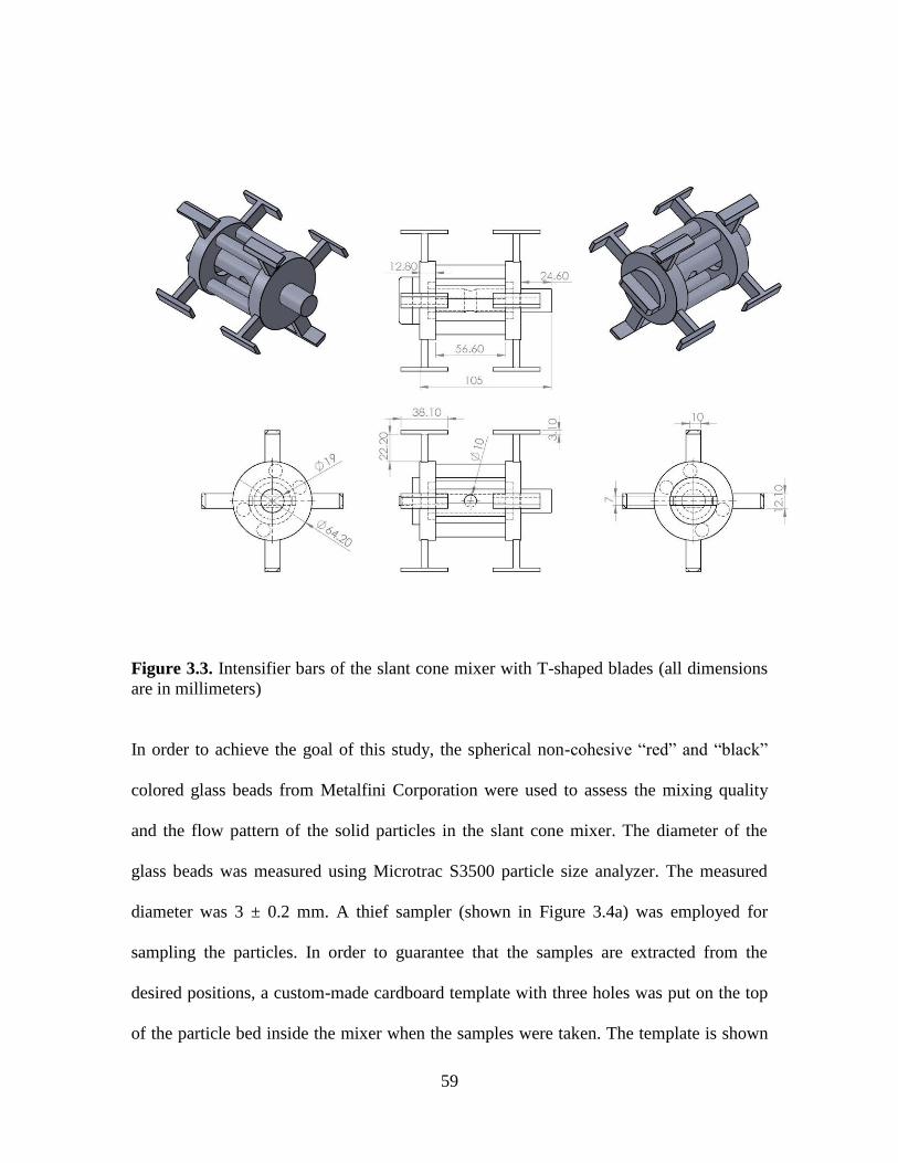
59

Figure 3.3. Intensifier bars of the slant cone mixer with T-shaped blades (all dimensions

are in millimeters)

In order to achieve the goal of this study, the spherical non-cohesive “red” and “black”

colored glass beads from Metalfini Corporation were used to assess the mixing quality

and the flow pattern of the solid particles in the slant cone mixer. The diameter of the

glass beads was measured using Microtrac S3500 particle size analyzer. The measured

diameter was 3 ± 0.2 mm. A thief sampler (shown in Figure 3.4a) was employed for

sampling the particles. In order to guarantee that the samples are extracted from the

desired positions, a custom-made cardboard template with three holes was put on the top

of the particle bed inside the mixer when the samples were taken. The template is shown

60

in Figure 3.4b. Each sample had approximately 80-100 particles. The percentage of red

and black glass beads in each sample was determined manually by counting the number

of each particle. Moreover, a digital camera was employed to capture the mixing of the

red and black solid particles. These snapshots and the sampling data were compared to

the simulations results to validate the DEM model developed in this study for the mixing

of the solid particles inside the slant cone mixer.

(a)

(b)

Figure 3.4.(a) Thief sampler and (b) Cardboard template

61

3.3 Discrete Element Method (DEM)

DEM was utilized for the study of slope stability obstacles and granular flow simulations

by Cundall and Strack (1979), who were the pioneers of DEM technology and

subsequently, it was applied in diverse simulations in various fields such as granular

mixing, dragline excavation, and silo filling(Asmar et al., 2002; Cleary, 1998; Holst et al.,

1999; Mishra and Rajamani, 1992; Rhodes et al., 2001). To delve into analysis wisely,

this technology is based on Newton’s laws, particularly Newton’s second law, and tracks

the motion of each particle in the system along with interactions of each particle with

other particles and the boundary (Arratia et al., 2006).

Admittedly, DEM is a popular, accurate, and costly numerical simulation procedure to

predict the solid particles behaviour. The high expenditure of DEM technology is relative

to different aspects. Firstly, the huge number of time step required to obtain the adequate

precision of the particle motions in a system. Secondly, it depends on the cost to

determine the contact force between particle and particle, and between particle and

boundary in each time intervals. In order to find optimization between CPU time and

numerical error, a proper time step ought to be considered in practice (Lemieux et al.,

2008).

As mentioned, in DEM simulation of the solid particles, Newton’s second law is used to

determine the position of each particle in each time step. Combination of contact

force( ) and gravity force ( ) is the total force which is applied to the particles.

62

Basically, the contact force is composed of a normal ( ) and a tangential force ( ) as

follows (Chaikittisilp et al., 2006):

( 3.1)

Although abundant models have been developed for the normal and tangential forces for

DEM simulations, Hertz-Mindlin contact force was employed for this study because this

model is easy to apply. Hertz (1882) developed a nonlinear model for the elastic contacts.

Several contact force models have been developed based on his theory. The entire of

these models are exploited the analogous procedures as Hertz model with limiting the

elastic contacts. Hertz (1882), and Mindlin and Deresiewicz (1953) proposed an equation

for the nonlinear elastic model as follow (Kruggel-Emden et al., 2007; Kruggel-Emden et

al., 2008)

(

( ) ( )

)√

( √

)

( 3.2)

√

√ √ ( )

( 3.3)

( 3.4)

√

√ √ ( )

( 3.5)

63

( )

[ (

| |

| |)

]

( 3.6)

where, , , , , , m , , , and are normal force, normal damping force,

normal stiffness, relative normal velocity, coefficient of restitution , mass of each particle,

displacement rate (normal overlap), shear modulus, Poisson ratio, and radius of the

particle, respectively. In addition, when normal displacement is constant and tangential

displacement varies, the tangential force is modeled using the above equation (Kruggel-

Emden et al., 2008; Mindlin and Deresiewicz, 1953), where presents the tangential

force, is the tangential damping force, shows the tangential stiffness , denotes the

tangential displacement, is the relative tangential velocity , is poison’s ratio,

presents the coefficient of the static friction, and is the contact area of two contacted

particles. Note that Hertz-Mindlin contact force model is used as normal and tangential

interactions in all simulations in this study.

Various influential aspects can change the result of DEM simulations. Particle inertial

properties (e.g. size, shape, and density), mechanical properties (e.g. stiffness, elasticity,

and plasticity), interactions of particles with particles, and interaction of particles with

boundary surfaces are examples of these aspects. Additionally, the selection of contact

models has a noticeable effect on these interactions, which are involved diverse factors

(e.g. restitution, friction, and cohesion), and several forces (e.g. gravity, electrostatic, and

magnetic). The physical and mechanical properties of the glass beads particles were

extracted from the literature and are listed in Table 3.1.

64

Table 3.1. Parameters used in DEM simulations

Parameter Value

Particle density (kg/ ) 2500

Particle shear modulus (Pa) 2.16×

Particle Poisson's ratio 0.3

Vessel density (kg/ ) 7850

Vessel shear modulus (Pa) 7×

Vessel Poisson's ratio 0.3

Particle–particle static friction coefficient 0.5

Particle–particle rolling friction coefficient 0.05

Particle–vessel static friction coefficient 0.4

Particle–vessel rolling friction coefficient 0.05

Particle–particle restitution coefficient 0.3

Particle–vessel restitution coefficient 0.3

In this study, Lacey index was used as a factor to find the mixing efficiency. Lacey index

is a statistical tool developed by Lacey (1956) in order to provide a mathematical

understanding of the mixing efficiency in a binary system. Following are the

mathematical equations included with Lacey method:

( 3.7)

where is the variance of the mixture

∑(

)

( 3.8)

is the variance in a completely segregated system

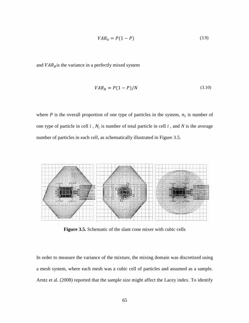
65

( )

( 3.9)

and is the variance in a perfectly mixed system

( )

( 3.10)

where P is the overall proportion of one type of particles in the system, is number of

one type of particle in cell i , is number of total particle in cell i , and N is the average

number of particles in each cell, as schematically illustrated in Figure 3.5.

Figure 3.5. Schematic of the slant cone mixer with cubic cells

In order to measure the variance of the mixture, the mixing domain was discretized using

a mesh system, where each mesh was a cubic cell of particles and assumed as a sample.

Arntz et al. (2008) reported that the sample size might affect the Lacey index. To identify

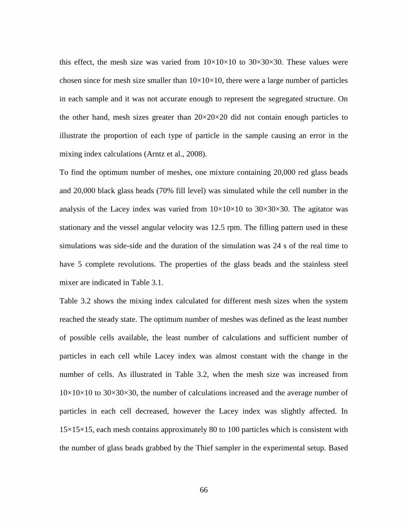
66

this effect, the mesh size was varied from 10×10×10 to 30×30×30. These values were

chosen since for mesh size smaller than 10×10×10, there were a large number of particles

in each sample and it was not accurate enough to represent the segregated structure. On

the other hand, mesh sizes greater than 20×20×20 did not contain enough particles to

illustrate the proportion of each type of particle in the sample causing an error in the

mixing index calculations (Arntz et al., 2008).

To find the optimum number of meshes, one mixture containing 20,000 red glass beads

and 20,000 black glass beads (70% fill level) was simulated while the cell number in the

analysis of the Lacey index was varied from 10×10×10 to 30×30×30. The agitator was

stationary and the vessel angular velocity was 12.5 rpm. The filling pattern used in these

simulations was side-side and the duration of the simulation was 24 s of the real time to

have 5 complete revolutions. The properties of the glass beads and the stainless steel

mixer are indicated in Table 3.1.

Table 3.2 shows the mixing index calculated for different mesh sizes when the system

reached the steady state. The optimum number of meshes was defined as the least number

of possible cells available, the least number of calculations and sufficient number of

particles in each cell while Lacey index was almost constant with the change in the

number of cells. As illustrated in Table 3.2, when the mesh size was increased from

10×10×10 to 30×30×30, the number of calculations increased and the average number of

particles in each cell decreased, however the Lacey index was slightly affected. In

15×15×15, each mesh contains approximately 80 to 100 particles which is consistent with

the number of glass beads grabbed by the Thief sampler in the experimental setup. Based

67

on the simulations, 15×15×15 was the optimum mesh system and was used for the rest of

the analysis.

In the calculation of variance, if the total number of the particles present in a sample was

below the average number of particles in all the samples, that sample was eliminated from

the calculations. The reason is that the small number of particles in cells can inaccurately

change the variance by a large number (Chandratilleke et al., 2012).

Table 3.2. Variety of mixing index for mesh sizes of 10×10×10 to 30×30×30.

Mesh size Number of cells Average number of

particle in each cell

Mixing index

10×10×10 1000 220 0.997453

11×11×11 1331 175 0.990395

12×12×12 1728 139 0.990242

13×13×13 2197 119 0.988382

14×14×14 2744 97 0.988101

15×15×15 3375 82 0.985736

16×16×16 4096 71 0.985462

17×17×17 4913 60 0.98204

18×18×18 5832 53 0.979002

19×19×19 6859 47 0.978474

20×20×20 8000 42 0.975198

21×21×21 9261 35 0.973106

22×22×22 10648 31 0.969812

23×23×23 12167 28 0.967471

24×24×24 13824 25 0.96511

25×25×25 15625 21 0.960273

26×26×26 17576 20 0.957099

27×27×27 19683 19 0.952443

28×28×28 21952 17 0.943947

29×29×29 24389 15 0.944374

30×30×30 27000 12 0.934869

68

The flow behavior of the particles inside the slant cone mixer was modeled using a

commercial DEM package called EDEM (DEM Solutions Ltd; United Kingdom;

Version: 2.5). The effects of the initial loading method (back-front, side-side, and top-

bottom), drum speed (5 rpm, 12.5 rpm, and 20 rpm), fill level (25%, 70%, and 100%),

and agitator speed (0 rpm, +100 rpm, -100 rpm, +200 rpm, and -200 rpm), on the mixing

efficiency was explored using DEM. Four processors were used for all the simulations

according to the availability of EDEM computational license. CPU times for simulations

were between 24 hours to 96 hours for 24 seconds of the real time. Moreover, the mixer

was filled while the vessel and agitator were motionless.

3.4 Results and Discussion

3.4.1 Model Validation

To validate the DEM model, the simulation results were compared to the experimental

data qualitatively and quantitatively. For the validation tests, the mixer was filled using

the side-side initial loading method with 47,000 red and 47,000 black glass beads with a

diameter of 3±0.2 mm (normal distribution) to achieve 70% of the fill level

approximately. The angular velocity of the drum was 12.5 rpm. To obtain the side-side

loading, a cardboard plate was inserted perpendicular to the axis of the blender rotation.

This cardboard divided the blender into two sections which have the same volume. Then,

one section was filled with the black glass beads and the other was filled with the red

glass beads. This experiment lasted for 24 s of the real time to obtain 5 complete

revolutions.

69

To validate the simulation results using imaging method, images of the solid mixture

were taken at the end of each complete revolution and then compared to the

corresponding simulation snapshots. As illustrated in Figure 3.7, there is a good

qualitative agreement between the experimental and simulation data.

Figure 3.6 shows the Lacey index after each revolution. It can be seen that a good

agreement was also achieved between the simulation results and the experimentally

determined values. These comparisons show that all the simulations are valid and

accurate since the gained results are almost the same for experiment and simulation in this

section.

Figure 3.6. Comparison between the Lacey index achieved through the experiment and

simulation at the fill level of 70%, the drum speed of 12.5 rpm and the side-side initial

loading while the agitator was stationary.

0

0.1

0.2

0.3

0.4

0.5

0.6

0.7

0.8

0.9

1

0 1 2 3 4 5 6

La

cey

In

dex

Number of Revolutions

Experiment

Simulation

70

Figure 3.7. Comparison between the snapshots of the simulated and real solid mixtures at

each revolution at the fill level of 70%, drum speed of 12.5 rpm and side-side initial

loading while the agitator was stationary.

71

3.4.2 Effect of Initial Loading

The effect of initial loading (i.e. side-side, top-bottom, and back-front) on the mixing

efficiency of the slant cone mixer was explored. In order to achieve this goal, 20,000 red

colored non-cohesive glass beads were mixed with 20,000 black colored non-cohesive

glass beads to reach 70% of the fill level of the mixer’s geometry. The diameter of the

glass beads was 4 mm and the angular velocity of the blender was 12.5 rpm to have 5

complete revolutions in 24 seconds of the real time. Moreover, the agitator was chosen to

be stationary, since the tumbling effect was of the interest at this part of this study.

Figure 3.8 depicts the Lacey mixing index versus time computed for the three different

initial loadings.

Figure 3.8. Mixing index versus time for different initial loading at the fill level of 70%

and the drum speed of 12.5 rpm while the agitator was stationary.

0

0.1

0.2

0.3

0.4

0.5

0.6

0.7

0.8

0.9

1

0 5 10 15 20 25

Mix

ing

In

dex

(-)

Time (s)

Top-Bottom Side-Side Back-Front

72

It can be seen that the side-side and top-bottom loadings nearly provided the same

mixing efficiency and they were both more efficient than the back-front loading.

According to these data, after 12 seconds, the mixing index values for both side-side and

top-bottom were over 0.90, whereas this value for the back-front was near 0.35. The

reason for the low mixing efficiency in the back-front case was that the movement paths

of each set of particles (red or black) were perpendicular to the expected paths for mixing;

as a result each set of particles was mixed with the same set instead of being mixed with

another set of the particles. In other words, the homogenization process was extremely

dependent on the dispersive transport, which is a slow process (Arratia et al., 2006).

From Figure 3.8 it can be seen that the mixing index at t = 0 s for the top-bottom loading

was higher than those for the back-front and side-side loading patterns. This result may be

ascribed to a larger initial contact surface between the red and black particles in the top-

bottom pattern compared to the other two loadings. This phenomenon is highlighted in

Figure 3.9, which shows the snapshots of the slant cone mixer simulations for three

different loading patterns at times equal to 0, 12, and 24 seconds.

Previous researchers explored the effect of the initial loading for the symmetrical

tumbling mixer such as the double cone, bin blender, v-blender, and pan coater. Our

results show the effect of the initial loading for the slant cone mixer, which is an

asymmetrical tumbling mixer. Moakher et al. (2000) studied the double-cone mixer and

V-blender. They showed that the top-bottom initial loading had a higher mixing

efficiency than the back-front loading. Aratia et al. (2006) explored the performance of

the bin blender and reported that the top-bottom initial loading was more efficient than

the back-front loading. The mixing of the Pan coater was also investigated by Sahni et al.

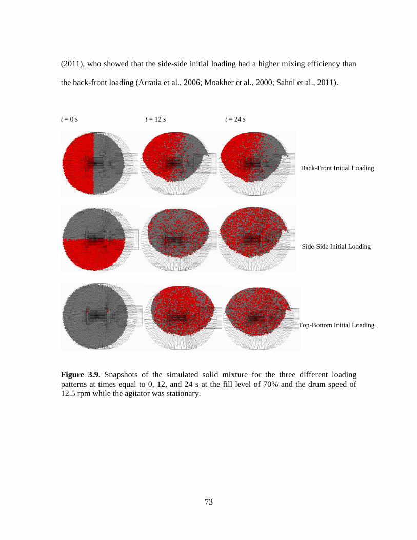
73

(2011), who showed that the side-side initial loading had a higher mixing efficiency than

the back-front loading (Arratia et al., 2006; Moakher et al., 2000; Sahni et al., 2011).

t = 0 s t = 12 s t = 24 s

Figure 3.9. Snapshots of the simulated solid mixture for the three different loading

patterns at times equal to 0, 12, and 24 s at the fill level of 70% and the drum speed of

12.5 rpm while the agitator was stationary.

Back-Front Initial Loading

Side-Side Initial Loading

Top-Bottom Initial Loading

74

3.4.3 Effect of the Vessel Speed

Next, we employed DEM to study the effect of the blender angular velocity on the mixing

efficiency of the slant cone mixer. The rotational speed was varied from 5 rpm to 20 rpm.

In these simulations, the side-side initial loading was used to charge 20,000 black and

20,000 red glass beads into the vessel. The fill level was approximately 70% and the

diameter of the glass beads was 4 mm. The agitator inside the blender was stationary

since the main objective of this part of the study was to assess the effect of the rotational

velocity of the drum.

Figure 3.10. Mixing index versus time for different speed of vessel at the fill level of

70% and the side-side initial loading while the agitator was stationary.

0

0.1

0.2

0.3

0.4

0.5

0.6

0.7

0.8

0.9

1

0 5 10 15 20 25

Mix

ing

In

dex

(-)

Time (s)

5 rpm 12.5 rpm 20 rpm

75

Figure 3.10 plots the Lacey mixing index versus time for three different blender rotational

speeds (5, 12.5, and 20 rpm). It can be seen that an increase in the angular velocity

enhanced the mixing index. It should be noted that the mixing indices at the 12.5 and 20

rpm reached 90% after 12 seconds, whereas the mixing index at 5 rpm reached 70% after

the same time period. Also, mixing index at 5 rpm reached 90% after 24 seconds.

Determination of the optimal angular velocity for a mixer is a challenging task because at

the lower angular velocities, the blender cannot provide the required cascading motion

and shear rates resulting in lower efficiency of the mixing. On the other hand, at the

higher angular velocity, the blender might provide enough centrifugal force to hold the

particles on the blender walls. Moreover, at the higher velocities, the mixer might not be

able to transfer its energy to the particles preventing them from tumbling freely and as a

result the particles are kept at the bottom of the mixer. In both cases, the mixing

efficiency can get reduced (Lemieux et al., 2008; Sahni et al., 2011).

As shown in Figure 3.10, the difference in mixing performances between the low and

medium angular velocities was larger than that between the medium and high angular

velocities. The reason behind this fact is that after one desirable speed, particles have

enough energy to move and the mixing efficiency depends only on the shear rate.

Although at a higher rotational velocity a better mixing efficiency is achieved, more

energy is consumed and more maintenance may be needed for the mixer. A future study

for this type of the mixer can be focused on the optimization of the rotational velocity for

the vessel in order to achieve the best mixing efficiency with less energy consumption

and less maintenance costs of the mixer.

76

In this study, an investigation regarding the transmitted energy from the slant cone mixer

to the particles by the rotor was also conducted. The average kinetic energies for all

particles at three different rotational speeds were obtained for the time domain of 0–24 s

using DEM. Figure 3.11 shows the increased kinetic energy of the particles at various

speeds of the vessel as a function of time. These results demonstrate that the average

value and amplitude of the increased kinetic energy was increased proportionally with the

vessel’s speed, since at higher rotational speeds, stronger force was applied to the

particles by the rotor (Iwasaki et al., 2001). The average kinetic energy (E) from t = 0 to t

= 24 s was calculated using the following equation:

∫

( 3.11)

E values calculated at 5 rpm, 12.5 rpm, and 20 rpm were 0.012978 J, 0.048411 J, and

0.091266 J, respectively.

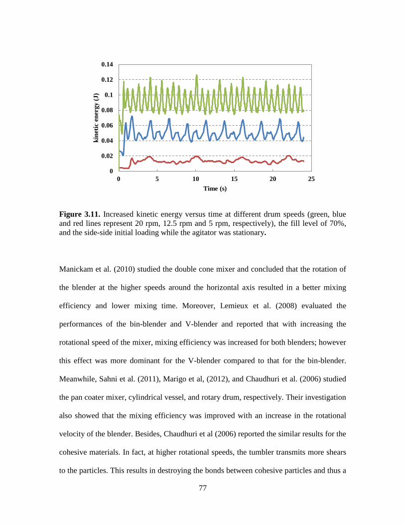
77

Figure 3.11. Increased kinetic energy versus time at different drum speeds (green, blue

and red lines represent 20 rpm, 12.5 rpm and 5 rpm, respectively), the fill level of 70%,

and the side-side initial loading while the agitator was stationary.

Manickam et al. (2010) studied the double cone mixer and concluded that the rotation of

the blender at the higher speeds around the horizontal axis resulted in a better mixing

efficiency and lower mixing time. Moreover, Lemieux et al. (2008) evaluated the

performances of the bin-blender and V-blender and reported that with increasing the

rotational speed of the mixer, mixing efficiency was increased for both blenders; however

this effect was more dominant for the V-blender compared to that for the bin-blender.

Meanwhile, Sahni et al. (2011), Marigo et al, (2012), and Chaudhuri et al. (2006) studied

the pan coater mixer, cylindrical vessel, and rotary drum, respectively. Their investigation

also showed that the mixing efficiency was improved with an increase in the rotational

velocity of the blender. Besides, Chaudhuri et al (2006) reported the similar results for the

cohesive materials. In fact, at higher rotational speeds, the tumbler transmits more shears

to the particles. This results in destroying the bonds between cohesive particles and thus a

0

0.02

0.04

0.06

0.08

0.1

0.12

0.14

0 5 10 15 20 25

kin

etic

en

erg

y (

J)

Time (s)

78

better mixing efficiency (Chaudhuri et al., 2006; Lemieux et al., 2008; Manickam et al.,

2010; Marigo et al., 2012; Sahni et al., 2011).

3.4.4 Effect of the Fill Level

In order to study the effect of fill level on the performance of the slant cone mixer,

simulations were performed for 30%, 70%, and 100% of fill level. In these simulations,

the initial loading method was the side-side with the particle diameter of 4mm. The

vessel’s angular velocity was 12.5 rpm and the agitator was stationary. The total number

of particles used in each simulation in order to achieve the approximated fill level has

been listed in Table 3.3.

Table 3.3. Total number of particles used in each simulation

Fill level Total number of particles

30% Fill level 10,000

70% Fill level 40,000

100% Fill level 100,000

79

Figure 3.12. Mixing index versus time at different fill levels, the drum speed of 12.5 rpm,

and the side-side initial loading while the agitator was stationary.

Figure 3.12 shows the Lacey mixing index as a function of time for three different fill

levels. According to these data, the slant cone mixer provided a better performance at

70% fill level compared to those achieved at 30% and 100% fill levels. This was due to

the fact that at the low fill level (30%), the rotor forced the particle bed to turn quicker

than the vessel, causing the particle bed to move as a bulk. On the other hand, at the high

fill level (100%) a less active bed and low mixing efficiency were attained. In other

words, at the higher fill levels, particles had low velocity and less space to move (Arratia

et al., 2006). Therefore, the medium fill level was the optimum in cases where the agitator

was stationary. This fill level was also recommended by Gemco (the manufacturer of the

slant cone mixer). It must be mentioned that the fill level is based on the volume occupied

by the particles not the mass of the bulk. In order to find the desired fill level, Gemco

0

0.1

0.2

0.3

0.4

0.5

0.6

0.7

0.8

0.9

1

0 5 10 15 20 25

Mix

ing

In

dex

(-)

Time (s)

30% Fill level 70% Fill level 100% Fill level

80

manufacturer prepared a guideline for the fill level of the slant cone mixer shown in

Figure 3.13.The average kinetic energy was also calculated for various fill levels and the

results are illustrated in Figure 3.14. It can be seen that at the higher fill levels, more

average kinetic energy was delivered to the particles due to the larger bulk mass inside

the vessel. The average kinetic energy for low, medium, and high fill levels, calculated by

Eqn. ( 3.11), were 0.006917 J, 0.048411 J, and 0.125642 J, respectively for a time span of

0 to 24 s. Arratia et al (2006) investigated the fill levels of 40%, 60%, and 80 % for a bin

blender with both top-bottom and side-side initial loading at 10 rpm and showed that the

mixing efficiency achieved at the lower levels was higher than that at the higher levels.

Arntz et al. (2008) studied the effect of the fill level for a rotary drum and found that the

optimum fill level for the drum rotating at 1.57 rad/s was 65 %. However, Manickam et

al. (2010) studied the effect of fill level on the mixing performance of a double cone

mixer. They did not observe any changes in the mixing efficiency when the fill level was

varied from 10% to 40%. Finally, Sahni et al. (2011) analyzed the fill level effect (21%,

37%, and 48 %) for a pan coater and reported that the fill level had an insignificant effect

on the mixing efficiency.

81

Figure 3.13. Fill level guideline for the slant cone mixer

Figure 3.14.Kinetic energy of solid particles versus time at different fill levels (green,

blue and red lines represent 100%, 70% and 30% fill level, respectively), the drum speed

of 12.5 rpm, and the side-side initial loading while the agitator was stationary.

0

0.02

0.04

0.06

0.08

0.1

0.12

0.14

0.16

0.18

0 5 10 15 20 25

kin

etic

en

erg

y (

J)

Time(s)

82

3.4.5 Effect of the Agitator Speed

The use of an agitator installed inside a slant cone mixer depends on the batch size. In

fact, the agitator is utilized only when the blender is slightly overloaded. The use of an

agitator reduces the mixing time by applying more energy to the particles. In this part of

the study, the effect of the agitator speed on the performance of the slant cone mixer was

investigated. The agitator speeds employed in this study were 0, +100, -100, 200, and -

200 rpm while the rotational speed of the vessel was kept constant at 12.5 rpm. The

positive rpm means that the rotation mode was co-rotating (i.e. the directions of the

rotation of the agitator and the vessel were the same) and the negative rpm means that the

rotation mode was counter-rotating (i.e. the directions of the rotation of the agitator and

the vessel were opposite). In order to achieve approximately 100% fill level in these

simulations, 50,000 red and 50,000 black non-cohesive glass beads with a diameter of 4

mm were placed inside the vessel using the side-side initial loading method. Figure 3.15

plots the Lacey mixing index versus time at the different rotational speeds of the agitator.

Based on these results, the mixing quality was poor at 100% fill level with a stationary

agitator (0 rpm). However, with an increase in the agitator speed, the quality of mixing

was improved. These data also indicated that at the same agitator speed, the mixing

quality in co-rotating mode was better than that in the counter-rotating mode. This is in

agreement with the recommendation of Gemco, the manufacturer of the slant cone

blenders.

83

Figure 3.15.Mixing index versus time at the different agitator speeds, the fill level of

100%, the drum speed of 12.5 rpm and the side-side initial loading while the agitator was

stationary.

Figure 3.16 shows the velocity of the particles in slant cone mixer when agitator rotates in

co-rotating and counter-rotating modes at 200 rpm while the drum speed was 12.5 rpm.

As can be seen, the particles near the agitator have the highest velocity, however in

counter-rotating mode the velocities of the particles near the agitator were less than those

achieved in the co-rotating mode. This could be justified by Newton’s second law of

motion. The total momentum of each particle is the vector sum of the momentums

applied by the agitator and the vessel. In the counter-rotating mode, since these vectors

are in opposite directions, sum of the momentum results in a smaller magnitude than that

in the co-rotating mode. As a result, the average velocity of the particle near the agitator

was higher in the co-rotating mode. Since the mixing quality depends on the movement of

the particles, higher mixing index was achieved in the co-rotating mode.

0

0.1

0.2

0.3

0.4

0.5

0.6

0.7

0.8

0.9

1

0 5 10 15 20 25

Mix

ing

In

dex

(-)

Time (s)

+100 rpm +200 rpm -200 rpm -100 rpm 0 rpm

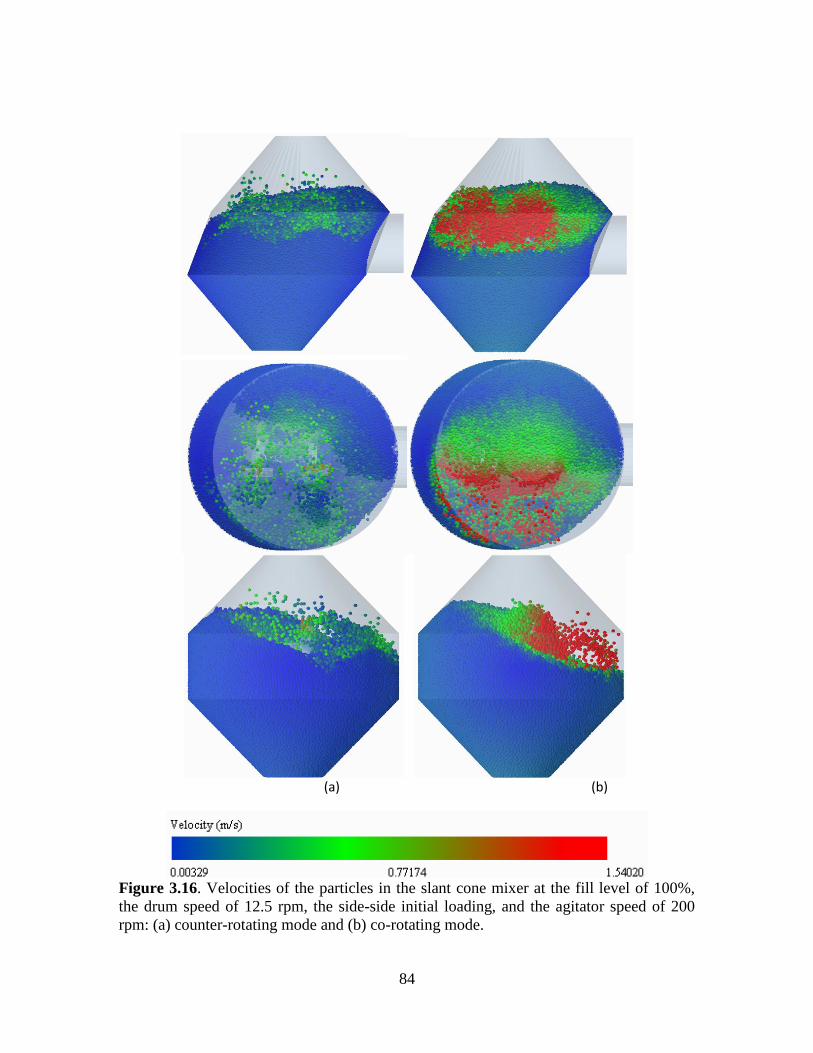
84

(a) (b)

Figure 3.16. Velocities of the particles in the slant cone mixer at the fill level of 100%,

the drum speed of 12.5 rpm, the side-side initial loading, and the agitator speed of 200

rpm: (a) counter-rotating mode and (b) co-rotating mode.

85

4. Analysis of the Mixing of Solid Particles in a Ploughshare

Mixer via Discrete Element Method (DEM)

4.1 Introduction

Various industries benefit from powder blending in the manufacturing of different

products such as pharmaceutical tablets, ceramic components, fertilizer blends, metal-

matrix composites, plastic parts, and food products. Nowadays, there are more complex

products in the market due to the progresses made in the powder mixing operations. As a

result, the development of the new techniques and theories, which enhance the

performance and assessment of the powder blending processes, is appreciated(Lu and

Hsiau, 2008; Wightman and Muzzio, 1998). The uniform mixing of solids is crucial due

to various reasons such as chemical reaction between the particles (e.g. in dry explosives)

and mechanical properties of the product (e.g. spatial distribution of different particles in

concrete). Furthermore, in some cases (e.g. pills and pharmaceutical powders), having a

fixed proportion of the materials is necessary (Paul et al., 2004). A critical issue in the

powder mixing is the evaluation of the mixing performance. To ensure the homogeneity

of the final product, characterisation of such systems plays an important role. In order to

measure the degree of homogeneity for a solid mixture, a mixing index is generally used.

A proper mixing index should be related closely to the specific characteristics of the final

mixture, independent of the mixing processes, and easy to determine. Nevertheless, so

far, over 40 different mixing indexes have been proposed by various authors. The number

86

of factors influencing the degree of mixing shows the complexity of the mixing process

and the difficulties in estimating the extent of homogeneity (Poux et al., 1991).

Industrial mixers can be broadly classified into the following categories (Poux et al.,

1991) : tumbling mixers, agitated mixers, pneumatic blenders, gravity silo blenders, high-

intensity mixers, and high-intimacy or high-shear mixers. In agitated blenders, particles

are mixed mechanically in a fixed-shell by using paddles, ploughs, or ribbons. Along with

the bulk mass, the mixing is achieved with the random movements of particles in agitated

mixers. In fact, the mixing is accomplished by both convection and shear in this type of

the mixers. In a common design of the agitated mixer, the agitating tools, which are

attached to a single or twin shaft, are rotated in a motionless shell, which could be vertical

or horizontal. Depending on the speed of the ploughs or paddles, the product is

mechanically sheared or fluidized and particles are tossed randomly. The agitated mixers

are frequently employed for the mixing of the solid particles including free-flowing

particles, cohesive particles, and pastes (Fuller, 1998; Kent, 2002; Ramponi et al., 2002).

The ploughshare mixer, which is categorized under agitated mixers, was considered as the

mixer in this study. Ploughshare mixer comprises a single or double U-shaped channel

and an impeller consisting of a single shaft or twin shafts carrying ploughs at a regular

pitch in between. The mixing of particles is achieved by lifting the solid particles,

generating chaotic motion, and shearing in the powder mass through the ploughs installed

on the mixer shaft. The powder motion causes convective mixing which its intensity is

proportional to the speed of the shaft. Ploughshare mixer is well-suited for the free

flowing to slightly cohesive powders.

87

This type of the blender has been utilized in different industries such as food, ceramics,

chemicals, building, plastics and pharmaceuticals. The main advantage of the plough

mixer is its compatibility with the solid particles of a wide range of densities. However,

this mixer is not suitable for very cohesive solids and higher plough speeds can result in

attrition. In addition, cleaning and emptying procedures are not easy (Paul et al., 2004).

So far, several studies regarding the ploughshare mixers have been published. However,

only a few of them used discrete element method (DEM) to analyze the flow pattern of

the solid particles in the ploughshare mixers. Some researchers used PEPT (positron

emission particle tracking) and found the flow pattern and average velocity of the

particles experimentally (Forrest et al., 2003; Jones and Bridgwater, 1998). Laurent and

Bridgwater (2002) studied the performance of the ploughshare mixer by PEPT and

showed that the axial dispersion coefficient changed linearly with the rotational speed of

the blade at lower than 50 rpm. Moreover, they demonstrated that a six-bladed agitator

provides better dispersion than a single-bladed mixer (Laurent and Bridgwater, 2002).

Laurent (2006) worked on characterization of the granular flow using PEPT method and

numerical simulation. He investigated the influence of the speed of the blade on the flow

pattern in the ploughshare mixer (Laurent, 2006). Jone et al. (2007) worked on flow

pattern within the ploughshare mixer and demonstrated that the mixing quality depended

on both the rotor frequency and the fill level. They found that the optimal fill level and

rotor frequency were 12.5- 25% and 4Hz, respectively for the batch process while, for

continues process, the optimal fill level and rotor frequency were 70% and 2Hz,

respectively (Jones et al., 2007). Laurent and Cleary (2012) utilized PEPT and DEM to

study the flow of the solid particles in a ploughshare mixer with one plough both

88

quantitatively and qualitatively. They reported good agreement between PEPT data and

DEM results (Laurent and Cleary, 2012). In the previous studies reported in the literature

regarding the mixing of the solid particles in the ploughshare mixers, the mixing indices

were not employed to assess the mixing quality of the binary system as a function of the

operating conditions and design parameters.

Thus, the objective of this study was to utilize DEM to calculate the mixing index as a

function of the initial loading, the rotational speed, fill level, and the particle size for a

six-blade ploughshare mixer. The experimental data reported by Laurent and Cleary

(2012) for the mean square of the axial and the radial displacements of the particles were

used to validate the DEM model developed in this study for the ploughshare mixer.

4.2 Specifications of the Mixer and Experimental Methods

In this study, DEM was employed to simulate the powder flow in the ploughshare

blender. Specifications of the ploughshare blender for the current study were similar to

the blender used by Laurent (2006). This mixer consisted of six long flat ploughs with

radial weirs, adjusted on a central shaft, to support the ploughs. The diameter of the

horizontal shell was 270 mm with a length of 650 mm. As shown in Figure 4.1, six

ploughs were installed on a shaft with a diameter of 30 mm. The space between the

adjacent ploughs was 105 mm while the angle was 90°. Moreover, Figure 4.2 shows the

dimensions of each plough. In current study, 7mm mono-sized glass bead was employed

as the particle during the simulations. Table 4.1 lists the parameters (properties of glass

bead and stainless steel) used in this study for DEM simulations. These data were

extracted from the literature (Zhou et al., 2004).

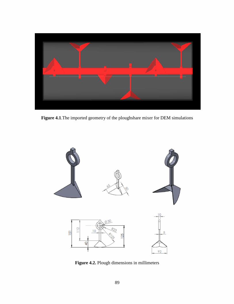
89

Figure 4.1.The imported geometry of the ploughshare mixer for DEM simulations

Figure 4.2. Plough dimensions in millimeters

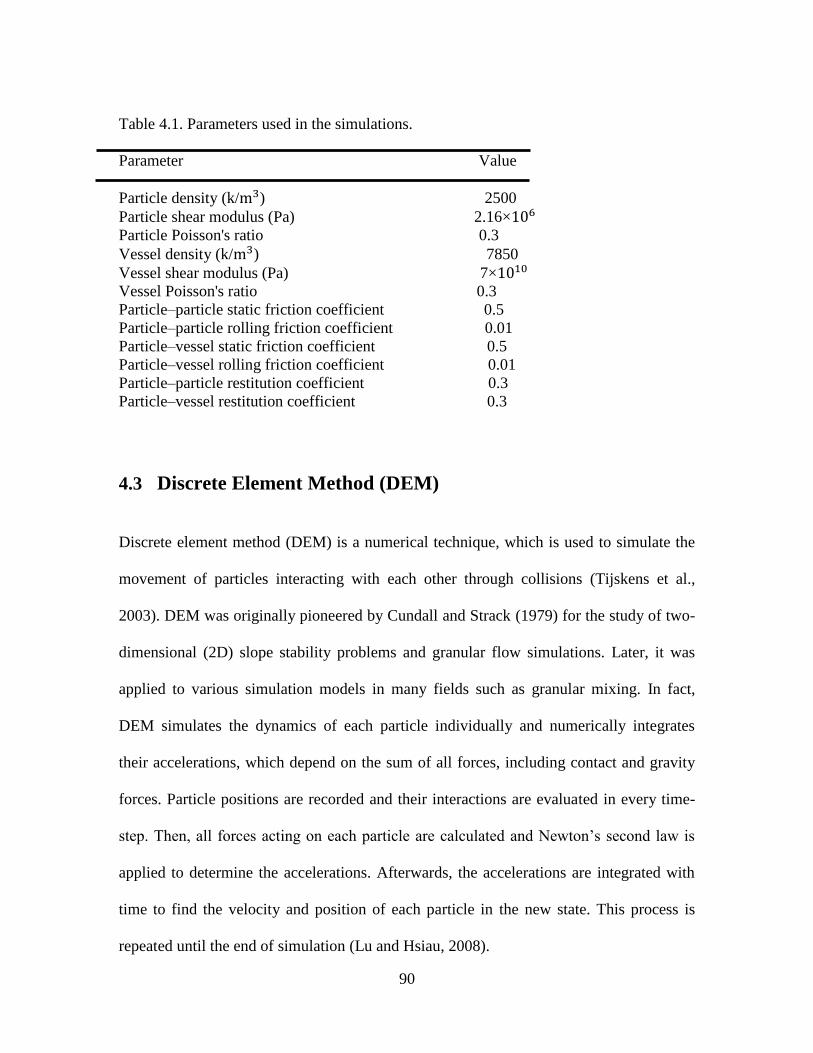
90

Table 4.1. Parameters used in the simulations.

Parameter Value

Particle density (k/ ) 2500

Particle shear modulus (Pa) 2.16×

Particle Poisson's ratio 0.3

Vessel density (k/ ) 7850

Vessel shear modulus (Pa) 7×

Vessel Poisson's ratio 0.3

Particle–particle static friction coefficient 0.5

Particle–particle rolling friction coefficient 0.01

Particle–vessel static friction coefficient 0.5

Particle–vessel rolling friction coefficient 0.01

Particle–particle restitution coefficient 0.3

Particle–vessel restitution coefficient 0.3

4.3 Discrete Element Method (DEM)

Discrete element method (DEM) is a numerical technique, which is used to simulate the

movement of particles interacting with each other through collisions (Tijskens et al.,

2003). DEM was originally pioneered by Cundall and Strack (1979) for the study of two-

dimensional (2D) slope stability problems and granular flow simulations. Later, it was

applied to various simulation models in many fields such as granular mixing. In fact,

DEM simulates the dynamics of each particle individually and numerically integrates

their accelerations, which depend on the sum of all forces, including contact and gravity

forces. Particle positions are recorded and their interactions are evaluated in every time-

step. Then, all forces acting on each particle are calculated and Newton’s second law is

applied to determine the accelerations. Afterwards, the accelerations are integrated with

time to find the velocity and position of each particle in the new state. This process is

repeated until the end of simulation (Lu and Hsiau, 2008).

91

Note that Hertz-Mindlin contact force model, which was described on page 55, is used as

normal and tangential interactions in all simulations of this study. In addition, in order to

calculate the mixing efficiency of the ploughshare mixer, Lacey (1954) index, which was

described on page 64, was utilized.

In order to measure the Lacey index (variance of the mixture), mixing domain was

discretized using a 10×10×15 mesh system (see Figure 4.3). Each mesh was a cubic cell

and contained approximately 45 to 50 particles. In the calculation of variance, if the total

number of the particles existed in a sample was below the average number of particles in

all the samples, that sample was eliminated from the calculations. This was due to the

fact that the small number of particles in cells can inaccurately change the variance to a

great extent (Chandratilleke et al., 2012).

Figure 4.3 . Schematic of the ploughshare mixer with cubic cells

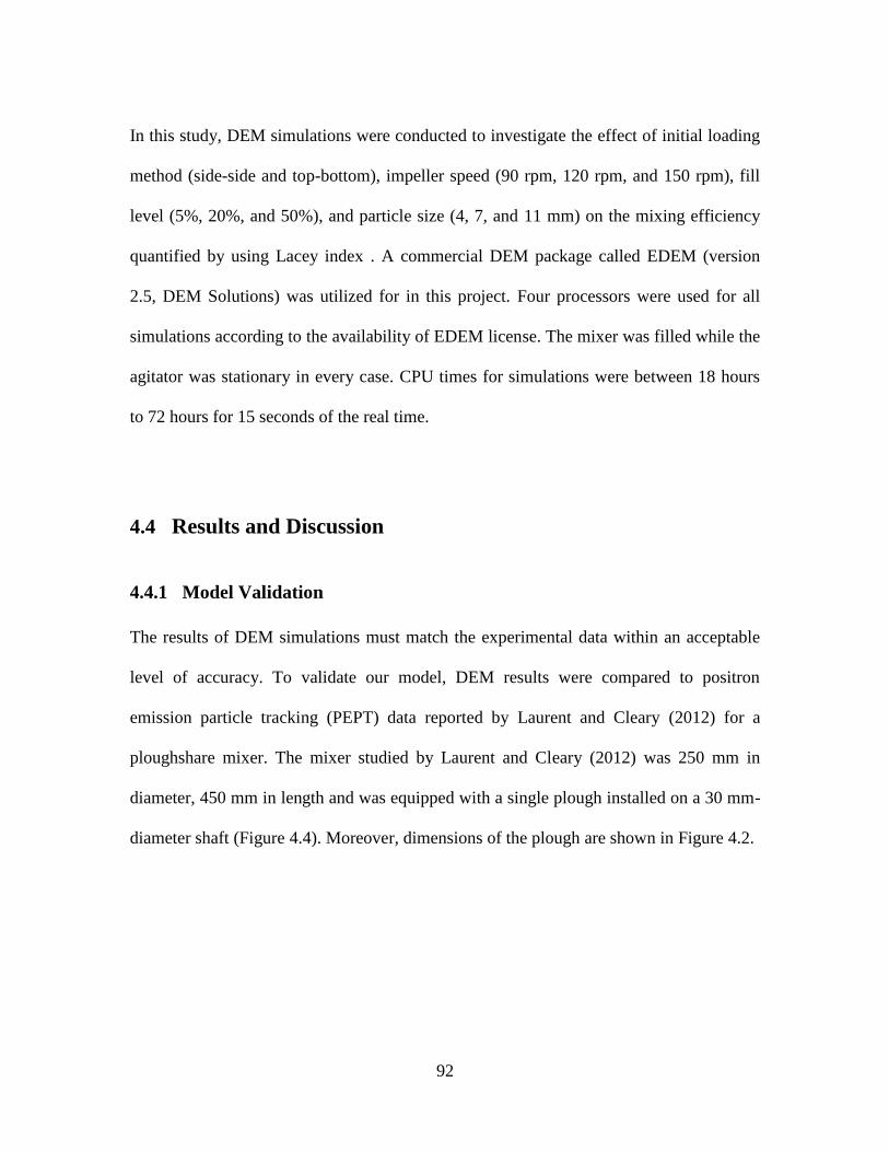
92

In this study, DEM simulations were conducted to investigate the effect of initial loading

method (side-side and top-bottom), impeller speed (90 rpm, 120 rpm, and 150 rpm), fill

level (5%, 20%, and 50%), and particle size (4, 7, and 11 mm) on the mixing efficiency

quantified by using Lacey index . A commercial DEM package called EDEM (version

2.5, DEM Solutions) was utilized for in this project. Four processors were used for all

simulations according to the availability of EDEM license. The mixer was filled while the

agitator was stationary in every case. CPU times for simulations were between 18 hours

to 72 hours for 15 seconds of the real time.

4.4 Results and Discussion

4.4.1 Model Validation

The results of DEM simulations must match the experimental data within an acceptable

level of accuracy. To validate our model, DEM results were compared to positron

emission particle tracking (PEPT) data reported by Laurent and Cleary (2012) for a

ploughshare mixer. The mixer studied by Laurent and Cleary (2012) was 250 mm in

diameter, 450 mm in length and was equipped with a single plough installed on a 30 mm-

diameter shaft (Figure 4.4). Moreover, dimensions of the plough are shown in Figure 4.2.

93

Figure 4.4. The imported geometry of the ploughshare mixer equipped with a single

plough for DEM simulations

In PEPT method, a single radioactive tracer is followed within the mass flow of the

granular material and the location of the tracer is monitored as a function of time. The

velocity distributions, shear gradients, and occupancy diagrams can be measured via

PEPT technique (Laurent and Bridgwater, 2002). Laurent and Cleary (2012) employed

PEPT technique to explore the flow of rice grains in a ploughshare mixer shown in Figure

4.4. The rice grains used in their study were approximately 2 by 4 mm with a density of

1400 kg/m3. However, they used a 2 mm in diameter glass sphere with a density of 2500

kg/m3 as the tracer in PEPT experiments. Therefore, the size, shape and density of the

tracer were different from those of the rice grains. Moreover, they used DEM simulation

for their study and compared flow patterns obtained from PEPT and DEM methods. In

their DEM modeling, the spherical particles with 2.5 to 3 mm diameter were used instead

of the rice grains employed in the PEPT method. In total, they used 103,000 particles to

achieve 25% of the mixer fill level. The coefficient of restitution and the coefficient of

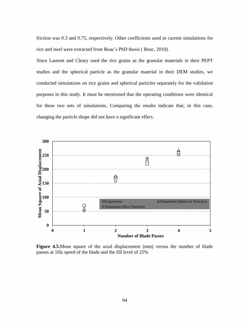
94

friction was 0.3 and 0.75, respectively. Other coefficients used in current simulations for

rice and steel were extracted from Boac’s PhD thesis ( Boac, 2010).

Since Laurent and Cleary used the rice grains as the granular materials in their PEPT

studies and the spherical particle as the granular material in their DEM studies, we

conducted simulations on rice grains and spherical particles separately for the validation

purposes in this study. It must be mentioned that the operating conditions were identical

for these two sets of simulations. Comparing the results indicate that, in this case,

changing the particle shape did not have a significant effect.

Figure 4.5.Mean square of the axial displacement (mm) versus the number of blade

passes at 1Hz speed of the blade and the fill level of 25%

0

50

100

150

200

250

300

0 1 2 3 4 5

Mea

n S

qu

are

of

Axia

l D

isp

lace

men

t

Number of Blade Passes

Experiment Simulation (Spherical Particles)

Simulation (Rice Particles)

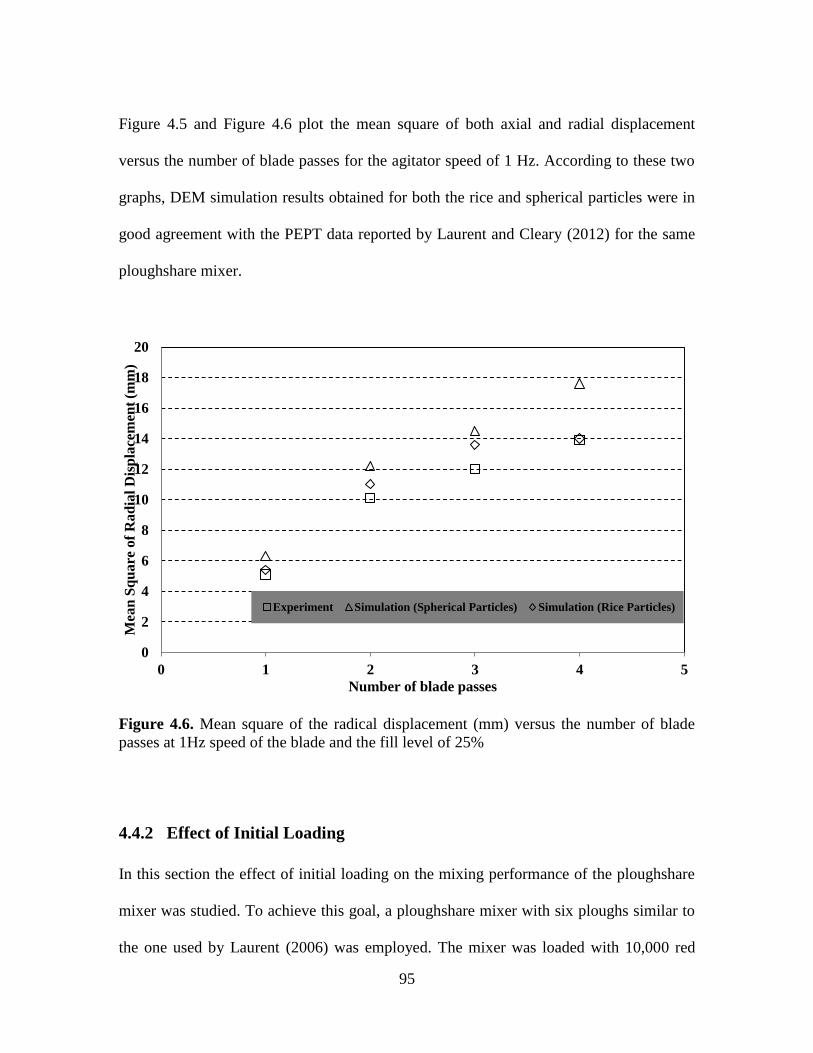
95

Figure 4.5 and Figure 4.6 plot the mean square of both axial and radial displacement

versus the number of blade passes for the agitator speed of 1 Hz. According to these two

graphs, DEM simulation results obtained for both the rice and spherical particles were in

good agreement with the PEPT data reported by Laurent and Cleary (2012) for the same

ploughshare mixer.

Figure 4.6. Mean square of the radical displacement (mm) versus the number of blade

passes at 1Hz speed of the blade and the fill level of 25%

4.4.2 Effect of Initial Loading

In this section the effect of initial loading on the mixing performance of the ploughshare

mixer was studied. To achieve this goal, a ploughshare mixer with six ploughs similar to

the one used by Laurent (2006) was employed. The mixer was loaded with 10,000 red

0

2

4

6

8

10

12

14

16

18

20

0 1 2 3 4 5

Mea

n S

qu

are

of

Rad

ial

Dis

pla

cem

ent

(mm

)

Number of blade passes

Experiment Simulation (Spherical Particles) Simulation (Rice Particles)

96

and 10,000 blue glass beads (7-mm diameter) to achieve the 20% fill level approximately.

Mixing lasted for 15 seconds while the agitator was rotating at 90 rpm. DEM model

parameters used for these simulations have been listed in Table 4.1 . Side-side initial

loading with different colored particles were compared to the top-bottom initial loading,

where these loadings were completely segregated at time equal to zero.

Figure 4.7. Mixing index versus time for different initial loading methods at the fill level

of 20% and the blade speed of 90 rpm

To assess the mixing quality as a function of the initial loading, Lacey index was

employed. Figure 4.7 depicts Lacey index versus time for both initial loading methods.

Slope = 0.225

Slope=0.206

0

0.1

0.2

0.3

0.4

0.5

0.6

0.7

0.8

0.9

1

0 1 2 3 4 5 6 7 8 9 10 11 12 13 14 15

Mix

ing I

nd

ex(-

)

Time (s)

Top-Bottom Side-Side

97

These results show that Lacey index ascended very fast at the beginning. However, the

rate of the change decreased after three seconds and the mixing index reached a plateau

after 10 seconds. These data also shows that the mixing indices were the same after 10

seconds for both loadings, however, prior to that, the top-bottom loading gave a better

mixing quality. Moreover, since for the top-bottom loading, the initial surface area

between the red and blue particles was larger than that for the side-side loading, Lacey

index was higher for the top-bottom loading at time zero. Although, at the beginning, the

mixing index was higher for the top-bottom loading, but it increased faster for the side-

side loading (see the slopes shown in Figure 4.7).

98

Figure 4.8. Snapshots of the simulated solid mixture at times equal to 0, 5, 10 and 15 s at

the fill level of 20% and the blade speed of 90 rpm for: (a) the side-side loading and (b)

the top-bottom loading.

Figure 4.8 illustrates the top snapshots of the ploughshare mixer for the two initial

loading at different times of the mixing process. As can be seen, at the beginning, the red

and blue particles were completely segregated. As the time passed, the glass bead

particles started to mix gradually, and at the end of the simulation, a solid mixture with a

high mixing quality was achieved. Previously, Chandratilleke et al. (2012) investigated

(a) (b)

99

the effect of the initial loading for another type of the agitated mixer, which consisted of a

vertical cylindrical vessel and a pair of flat blades (high shear mixer). Similar to our

results, they indicated that the initial loading affected the mixing rate, where the mixing

rate for the side-side loading was faster compared to that for the top-bottom initial

loading.

4.4.3 Effect of the Impeller Speed

The speed of the rotating blade affects the granular flow in the ploughshare mixer;

however, in order to achieve an acceptable particle movement or shear rate, the low

rotational speeds have to be avoided. On the other hand, a high rotational speed may

cause clutter; this may also increase the possibility of reducing the particles size and

damaging the wall due to throwing the powder. Thus, in order to have the proper mixing,

an optimum average speed needs to be applied. To examine the effect of the impeller

speed, the rotational speeds of 90, 120 and 150 rpm were applied. Mixer was filled up to

20% of the fill level approximately with the side-side loading of 10,000 red and 10,000

blue glass beads (7 mm diameter).

Figure 4.9 shows the Lacey index versus time as a function of the agitator speed. It can be

seen that the mixing indices reached a plateau at all impeller speeds. However, Lacey

index reached its maximum value faster at the higher rotational speeds. Therefore, it is

undeniable that the blade speed has a significant effect on the mixing time. This is due to

the fact that, increasing the speed of blade, increases the movement of particles, resulting

in a better mixing performance. The mixing time can be defined as the time needed to

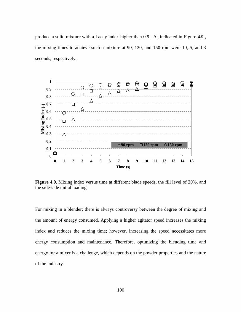
100

produce a solid mixture with a Lacey index higher than 0.9. As indicated in Figure 4.9 ,

the mixing times to achieve such a mixture at 90, 120, and 150 rpm were 10, 5, and 3

seconds, respectively.

Figure 4.9. Mixing index versus time at different blade speeds, the fill level of 20%, and

the side-side initial loading

For mixing in a blender; there is always controversy between the degree of mixing and

the amount of energy consumed. Applying a higher agitator speed increases the mixing

index and reduces the mixing time; however, increasing the speed necessitates more

energy consumption and maintenance. Therefore, optimizing the blending time and

energy for a mixer is a challenge, which depends on the powder properties and the nature

of the industry.

0

0.1

0.2

0.3

0.4

0.5

0.6

0.7

0.8

0.9

1

0 1 2 3 4 5 6 7 8 9 10 11 12 13 14 15

Mix

ing I

nd

ex (

-)

Time (s)

90 rpm 120 rpm 150 rpm

101

4.4.4 Effect of the Fill Level

The fill level in the mixer is an important factor in the mixing studies, mainly because it is

easily controlled and all industries rather to use the maximum capacity of the mixer

volume at an acceptable level of performance. On the other hand, if the fill level exceeds

a certain amount, mixing dead zones appear in the mixer especially at the top levels for

the agitated mixer, which is not desirable.

In order to examine the effect of the fill level on the mixing efficiency of the ploughshare

mixer, various simulations were conducted using three different fill levels. In these

simulations, the mixtures were agitated at the rotational speed of 90 rpm for 15 seconds.

To achieve approximately 5%, 20% and 50% of the fill level, 5,000, 20,000 and 50,000 7-

mm glass beads were employed, respectively. In every case, the total number of particles

was divided into two halves of two different colors filling the mixer using the side-side

loading method.

102

Figure 4.10. Mixing index versus time at different fill levels, the blade speed of 90 rpm,

and the side-side initial loading

Figure 4.10 plots the Lacey index versus time at various fill levels. According to these

results, fill level influenced the mixing efficiency considerably. It can be seen that the

lower fill levels resulted in the higher mixing indices. The mixing time at 90 rpm for 5%

fill level was 5 seconds, which was very fast. This value for 20% fill level increased to 10

seconds. Interestingly, at this agitator speed, the solid mixture with 50% fill level did not

reach the desired mixing index of 0.9 even after 15 seconds. Among these three fill levels,

it seems that the mixing performance achieved at 20% fill level was more efficient

considering the filling volume.

At the lower fill levels, since less number of particles is available, momentum of inertia

applied to each particle is higher, which leads to a higher particle velocity and thus a

0

0.1

0.2

0.3

0.4

0.5

0.6

0.7

0.8

0.9

1

0 1 2 3 4 5 6 7 8 9 10 11 12 13 14 15

Mix

ing

In

dex

(-)

Time (s)

50% Fill level 20% Fill level 5% Fill level

103

better mixing performance (Muzzio et al., 2008). Previously, Muzzio et al. (2008) and

Terashita et al. (2002) studied the effect of the fill level on the performances of the ribbon

blender and high shear mixers, respectively. Muzzio et al. (2008) found that for a 3-spoke

blade ribbon mixer, increasing the fill level decreased the homogeneity of the blend.

However, fill level does not seem to have a substantial influence in a 5-spoke blade

mixer. Terashita et al. (2002) investigated this effect for high shear mixers. They

concluded that, at the higher fill levels, the particles have less free space to move in the

agitating vessel. Moreover, they proposed 50% fill level as the optimum. At this fill level,

the particles had enough space to maintain the proper velocity, which resulted in the

adequate particle motion (Terashita et al., 2002).

4.4.5 Effect of the Particle Size

Particle size can affect the flow pattern and simulation time; smaller particles increase the

simulation time. As a result, particle size is a crucial factor in particulate simulations. In

order to investigate the effect of the particle size on the mixing quality in a ploughshare

mixer, several simulations were conducted with 4, 7, and 11 mm glass beads, filled by

side-side loading method at 120 rpm agitator speed.

To achieve approximately 20% fill level, the number of particles for 4, 7 and, 11 mm

were 107188, 20000, and 5155. These numbers were estimated based on the void fraction

between particles for each particle size. Moreover, in order to contain approximately 45

to 50 particles in each sample, mesh size for 4, 7 and 11 mm are 16×16×24, 10×10×15

and 5×5×8, respectively.

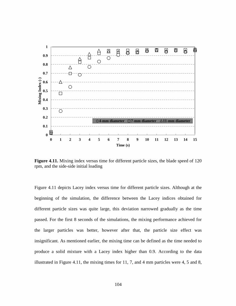
104

Figure 4.11. Mixing index versus time for different particle sizes, the blade speed of 120

rpm, and the side-side initial loading

Figure 4.11 depicts Lacey index versus time for different particle sizes. Although at the

beginning of the simulation, the difference between the Lacey indices obtained for

different particle sizes was quite large, this deviation narrowed gradually as the time

passed. For the first 8 seconds of the simulations, the mixing performance achieved for

the larger particles was better, however after that, the particle size effect was

insignificant. As mentioned earlier, the mixing time can be defined as the time needed to

produce a solid mixture with a Lacey index higher than 0.9. According to the data

illustrated in Figure 4.11, the mixing times for 11, 7, and 4 mm particles were 4, 5 and 8,

0

0.1

0.2

0.3

0.4

0.5

0.6

0.7

0.8

0.9

1

0 1 2 3 4 5 6 7 8 9 10 11 12 13 14 15

Mix

ing

In

dex

(-)

Time (s)

4-mm diameter 7-mm diameter 11-mm diameter

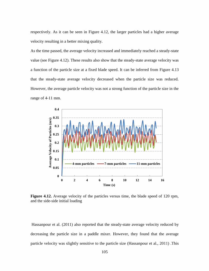
105

respectively. As it can be seen in Figure 4.12, the larger particles had a higher average

velocity resulting in a better mixing quality.

As the time passed, the average velocity increased and immediately reached a steady-state

value (see Figure 4.12). These results also show that the steady-state average velocity was

a function of the particle size at a fixed blade speed. It can be inferred from Figure 4.13

that the steady-state average velocity decreased when the particle size was reduced.

However, the average particle velocity was not a strong function of the particle size in the

range of 4-11 mm.

Figure 4.12. Average velocity of the particles versus time, the blade speed of 120 rpm,

and the side-side initial loading

Hassanpour et al. (2011) also reported that the steady-state average velocity reduced by

decreasing the particle size in a paddle mixer. However, they found that the average

particle velocity was slightly sensitive to the particle size (Hassanpour et al., 2011) .This

0

0.05

0.1

0.15

0.2

0.25

0.3

0.35

0.4

0 2 4 6 8 10 12 14 16

Av

era

ge

Vel

oci

ty o

f P

art

icle

s (m

/s)

Time (s)

4-mm particles 7-mm particles 11-mm particles

106

similarity may be due to the nature of both mixers. The paddle mixer and the ploughshare

mixer are classified under agitated mixers.

Figure 4.13. Average velocity of the particles versus particles size, the blade speed of

120 rpm, and the side-side initial loading

V = 0.0114 D + 0.1476

R² = 0.9999

0

0.05

0.1

0.15

0.2

0.25

0.3

0 2 4 6 8 10 12

Av

era

ge

Pa

rtic

le V

elo

city

(m

/s)

Particle diameter (mm)

107

5. CONCLUSIONS AND RECOMMENDATIONS FOR

FUTURE WORK

5.1 Conclusions

In the first part of this study, discrete element method (DEM), which is a powerful

technique for understanding the complex granular flow pattern, was employed to

characterize the mixing performance of the slant cone mixer as a function of the initial

loading pattern, drum speed, fill level, agitator speed, and rotation mode. The model

developed in this study was validated by experimental data obtained using sampling and

imaging methods. It was found that the side-side and top-bottom loadings nearly provided

the same mixing efficiency and both were more efficient than the back-front loading. An

increase in the angular velocity of vessel enhanced the mixing index. In fact, the average

value and amplitude of the kinetic energy of the solid particles increased proportionally

with the drum speed. The slant cone mixer provided a better performance at 70% fill level

compared to 30% and 100% fill levels when the agitator was stationary. Moreover, the

results demonstrated that the mixing quality was poor at 100% fill level with a stationary

agitator (0 rpm). However, increasing the agitator speed, improved the quality of mixing.

Our results also indicated that at the same agitator speed, the mixing quality achieved in

co-rotating mode was higher than that in the counter-rotating mode.

In the next part of this study, the discrete element method (DEM) was employed to

characterize the mixing performance of the ploughshare blender as a function of the

initial loading pattern, impeller speed, fill level, and particle size. The DEM results were

108

successfully validated using PEPT data reported in the literature. The data showed that

the mixing quality ascended very fast at the beginning of the blending process. However,

the rate of the change decreased after a few seconds and the mixing index reached a

plateau after 10 seconds. The mixing indices were the same after 10 seconds for both

side-side and top-bottom loadings, however, prior to that, the top-bottom loading gave a

better mixing quality. Although, at the beginning, the mixing index was higher for the

top-bottom loading, but it increased faster for the side-side loading. The mixing time,

which was defined as the time needed to produce a solid mixture with a mixing index

higher than 0.9, reduced with an increase in the rotational speed. It was found that the fill

level influenced the mixing efficiency considerably. The lower fill levels resulted in the

higher mixing indices. This was due to the fact at the higher fill levels, the particles had

less free space to move in the agitated vessel. The mixing time decreased with an increase

in the particle size. In fact, the larger particles had a higher average velocity resulting in a

better mixing quality. However, the average particle velocity was not a strong function of

the particle size in the range of 4 -11 mm.

Applying the findings of this study is expected to help engineers enhance the degree of

homogeneity of solid mixtures blended in the slant cone mixers and the ploughshare

mixers.

109

5.2 Recommendations for Future Work

The following recommendations are proposed for future studies:

Assess the performance of a slant cone blender in the mixing of binary mixtures

with the different size ratios

Evaluate the mixing performance of a slant cone blender in the mixing of poly-

disperse particles.

Determine the optimal operating conditions for a slant cone and ploughshare

mixers

Compare the performances of the slant cone and double cone blenders with same

volume and operating conditions

Explore the scale-up criteria for powder blenders

110

Nomenclature

Contact area of two contacted particles (m²)

Coefficient of static friction (-)

Contact force (N)

Normal damping force (N)

Tangential damping force (N)

Normal force (N)

Tangential force (N)

Shear modulus (Pa)

Mixing index (-)

Average number of particle in each cell (-)

Number of total particle in cell i (-)

Overall proportion of one type of particles in the

system (-)

Radius (mm)

Variance of the mixture (-)

Variance in a perfectly mixed system (-)

Variance in a completely segregated system (-)

Distance between two particle centers ( )

particle diameter ( )

coefficient of restitution (-)

111

Number of cell (-)

stiffness of a linear spring (

)

mass of particle ( )

reduced mass of the colliding bodies ( )

Normal stiffness (N/m)

Number of one type of particle in cell i (-)

tangential stiffness (N/m)

Relative normal velocity (m/s)

Relative tangential velocity (m/s)

tangential displacement (m)

Displacement rate (m/s)

Poison ratio (-)

112

GLOSSARY

Restitution coefficient Ratio of speed of separation to speed of approach in a

collision

Elastic spring force A force exerted by a spring onto the object stretching or

compressing it

Damping coefficient The measure of energy dissipation and the ratio of the force

over the velocity

Young’s modulus Ratio of shear stress to the shear strain

Loading period The period during which sample is subjected to a certain

stress

Unloading period The period of releasing sample from the stress

Coefficient of Rolling

Friction

Scalar value used to determine how much torque is needed to

be applied to an object of a given material at rest, on a flat

surface, to put it into motion

Coefficient of static

Friction

Scalar value used to determine how much force is required for

an object, of a given material, at rest on another known

substance, start to move. It is the ratio of the tangential force

required to produce sliding to the normal force between the

surfaces

Poisson's ratio

Ratio of transverse contraction strain to longitudinal extension

strain in the direction of stretching force

113

Bibliography:

Abouzeid, A.Z.M., Fuerstenau, D.W., 2010. Mixing-demixing of particulate solids in

rotating drums. International Journal of Mineral Processing 95, 40-46.

Ahmadian, H., Hassanpour, A., Ghadiri, M., 2011. Analysis of granule breakage in a

rotary mixing drum: Experimental study and distinct element analysis. Powder

Technology 210, 175-180

Alexander, A., Shinbrot, T., Johnson, B., Muzzio, F.J., 2004. V-blender segregation

patterns for free-flowing materials: effects of blender capacity and fill level. International

Journal of Pharmaceutics 269, 19-28.

Allen, M.P., Tildesley, D.J., 1987. Computer simulation of liquids. Clarendon

Press;Oxford University Press, Oxford [Oxfordshire] New York.

Allen, T., 1981. Particle size measurement, 3rd ed. Chapman and Hall, London ; New

York.

Arntz, M.M.H.D., den Otter, W.K., Briels, W.J., Bussmann, P.J.T., Beeftink, H.H.,

Boom, R.M., 2008. Granular Mixing and Segregation in a Horizontal Rotating Drum: A

Simulation Study on the Impact of Rotational Speed and Fill Level. AIChE Journal 54,

3133-3146.

Arratia, P.E., Duong, N.H., Muzzio, F.J., Godbole, P., Reynolds, S., 2006. A study of the

mixing and segregation mechanisms in the Bohle Tote blender via DEM simulations.

Powder Technology 164, 50-57.

Asmar, B.N., Langston, P.A., Matchett, A.J., 2002. A generalised mixing index in distinct

element method simulation of vibrated particulate beds. Granular Matter 4, 129-138.

Berman, J., Planchard, J.A., 1995. Blend Uniformity and Unit Dose Sampling. Drug

Development and Industrial Pharmacy 21, 1257-1283.

Berman, J., Schoeneman, A., Shelton, J.T., 1996. Unit dose sampling: A tale of two

thieves. Drug Development and Industrial Pharmacy 22, 1121-1132.

Bertrand, F., Leclaire, L.A., Levecque, G., 2005. DEM-based models for the mixing of

granular materials. Chemical Engineering Science 60, 2517-2531.

Bharadwaj, R., Ketterhagen, W. R., & Hancock, B. C., 2010. Discrete element simulation

study of a Freeman powder rheometer. Chemical Engineering Science, 65, 5747–5756.

114

Boac, G., 2010. Quality Changes, Dust Generation, And Commingling During Grain

Elevetor Handling, PhD thesis, Kansas State University, Manhattan, USA

Carreau, P.J., Patterson, I., Yap, C.Y., 1976. Mixing of Viscoelastic Fluids with Helical-

Ribbon Agitators .1. Mixing Time and Flow Patterns. Canadian Journal of Chemical

Engineering 54, 135-142.

Cavender, J., 2000. Quick, thorough and gentle blending with a vertical ribbon

mixer.Powder Bulk Eng. 14, 46-57.

Chaikittisilp, W., Taenumtrakul, T., Boonsuwan, P., Tanthapanichakoon, W.,

Charinpanitkul, T., 2006. Analysis of solid particle mixing in inclined fluidized beds

using DEM simulation. Chemical Engineering Journal 122, 21-29.

Chandratilleke, G.R., Yu, A.B., Bridgwater, J., Shinohara, K., 2012. A particle-scale

index in the quantification of mixing of particles. AIChE Journal 58, 1099-1118.

Chaudhuri, B., Mehrotra, A., Muzzio, F.J., Tomassone, M.S., 2006. Cohesive effects in

powder mixing in a tumbling blender. Powder Technology 165, 105-114.

Cleary, P.W., 1998. The filling of dragline buckets. Mathematical Engineering in Industry

7, 1-24.

Cleary, P. W., Sawley, M. L., 2002. DEM modeling of industrial granular flows: 3D case

studies and the effect of particle shape on hopper discharge. Applied Mathematical

Modelling 26, 89-111.

Cleary, P.W., Sawley, M.L., 2002. DEM modelling of industrial granular flows: 3D case

studies and the effect of particle shape on hopper discharge. Applied Mathematical

Modelling 26, 89-111.

Cleary, P. W., 2004. Large scale industrial DEM modeling. Journal of Engineering

computational 21, 169-204.

Cullen, P.J., 2009. Food mixing: principles and applications. Wiley-Blackwell,

Chichester, U.K. ; Ames, Iowa.

Cundall, P.A., Strack, O.D.L., 1980. A Discrete Numerical-Model for Granular

Assemblies - Reply. Geotechnique 30, 335-336.

Daumann, B., Nirschl, H., 2008. Assessment of the mixing efficiency of solid mixtures by

means of image analysis. Powder Technology 182, 415-423.

115

Deen, N.C., Willem, G., Sander, G., Kuipers, J.A.M., 2010. Numerical Analysis of Solids

Mixing in Pressurized Fluidized Beds. Industrial & Engineering Chemistry Research 49,

5246-5253.

Ding, Y.L., Forster, R., Seville, J.P.K., Parker, D.J., 2002. Granular motion in rotating

drums: bed turnover time and slumping-rolling transition. Powder Technology 124, 18-

27.

Ding, Y.L., Forster, R.N., Seville, J.P.K., Parker, D.J., 2001. Scaling relationships for

rotating drums. Chemical Engineering Science 56, 3737-3750.

Dubey, A., Sarkar, A. , Ierapetritou, M. , Wassgren, C.R., Muzzio, F.J., 2011. DEM based

approaches for studying the granular dynamics of continuous blending processes,

Macromolecular Materials and Engineering 296, 290–307.

Dury, C. M. Ristow, G. H., 1997. Radial segregation in a two-dimensional rotating drum.

Journal of physics. I, 7, 735-747.

Fan, L. T., Chen, S. J., Watson, C. A., 1970. Solids mixing. Industrial &

Engineering Chemistry Research 62, 53-69.

Forberg, H., 1992. Short note on modern mixing: theory and practice, Powder Handl.

Process. 4, 318-320.

Forrest, S., Bridgwater, J., Mort, P.R., Litster, J., Parker, D.J., 2003. Flow patterns in

granulating systems. Powder Technology 130, 91-96.

Fuller, W. O., 1998. Mixing up a batch: batch mixer types and selection tips, Powder

Bulk Eng. 12, 48-66.

Geng, F., Yuan, Z., Yan, Y., Luo, D., Wang, H., Li, B., Xu, D., 2009. Numerical

simulation on mixing kinetics of slender particles in a rotary dryer, Powder Technology

193 50–58.

Gopinath, S., Vedaraman, R., 1982. A Vibrating Mixer for Mixing Particulate Solids.

Research and Industry 27, 321-323.

Gotoh, K., Masuda, H., Higashitani, K., 1997. Powder technology handbook, 2nd ed.

Marcel Dekker, New York.

Hanes, D. M., Walton, O. R., 2000. Simulation and physical measurements of glass

spheres &owing down a bumpy incline. Powder Techlogy 109, 133 -144.

Harnby, N., 2000. An engineering view of pharmaceutical powder mixing. Pharm. Sci.

Technol. 3, 303-309.

116

Hassanpour, A., Tan, H.S., Bayly, A., Gopalkrishnan, P., Ng, B., Ghadiri, M., 2011.

Analysis of particle motion in a paddle mixer using Discrete Element Method (DEM).

Powder Technology 206, 189-194.

Hersey, J.A., 1975. Ordered Mixing - New Concept in Powder Mixing Practice. Powder

Technology 11, 41-44.

Hertz, H., 1882. Ueber die Berührung fester elastischer Koerper. Journal für die Reine

und Angewandte Mathematik 92, 156-171.

Hixon, L., Ruschmann, J., 1992. Using a conical screw mixer for more than mixing.

Powder Bulk Eng., 6, 37-43.

Hogg, R., Fuersten, Dw, 1972. Transverse Mixing in Rotating Cylinders. Powder

Technology 6, 139-&.

Holst, J.M.F.G., Rotter, J.M., Ooi, J.Y., Rong, G.H., 1999. Numerical modeling of silo

filling. II: Discrete element analyses. Journal of Engineering Mechanics-Asce 125, 104-

110.

Hoomans, B.P.B., Kuipers, J.A.M., van Swaaij, W.P.M., 2000. Granular dynamics

simulation of segregation phenomena in bubbling gas-fluidised beds. Powder Technology

109, 41-48.

Iwasaki, T., Satoh, M., Koga, T., 2001. Analysis of collision energy of bead media in a

high-speed elliptical-rotor-type powder mixer using the discrete element method. Powder

Technology 121, 239-248.

Jones, J.R., Bridgwater, J., 1998. A case study of particle mixing in a ploughshare mixer

using Positron Emission Particle Tracking. International Journal of Mineral Processing

53, 29-38.

Jones, J.R., Parker, D.J., Bridgwater, J., 2007. Axial mixing in a ploughshare mixer.

Powder Technology 178, 73-86.

Kaneko, Y., Shiojima, T., Horio, M., 2000. Numerical analysis of particle mixing

characteristics in a single helical ribbon agitator using DEM simulation. Powder

Technology 108, 55-64.

Kent, M., 2002. Mixer selection: an aid to those involved in the selection, specification

and purchasing of mixing machines. Powder Handl. Process, 14, 41-43

Khakhar, D.V., McCarthy, J.J., Gilchrist, J.F., Ottino, J.M., 1999. Chaotic mixing of

granular materials in two-dimensional tumbling mixers. Chaos 9, 195-205.

117

Kruggel-Emden, H., Simsek, E., Rickelt, S., Wirtz, S., Scherer, V., 2007. Review and

extension of normal force models for the Discrete Element Method. Powder Technology

171, 157-173.

Kruggel-Emden, H., Wirtz, S., Scherer, V., 2008. A study on tangential force laws

applicable to the discrete element method (DEM) for materials with viscoelastic or plastic

behavior. Chemical Engineering Science 63, 1523-1541.

Kuo, H.P., Knight, P.C., Parker, D.J., Seville, J.P.K., 2005. Solids circulation and axial

dispersion of cohesionless particles in a V-mixer. Powder Technology 152, 133-140.

Lacey, P., 1954. Developments in theory of particulate mixing. Journal of Applied

Chemistry 4, 257-259

Laurent, B.F.C., 2006. Scaling factors in granular flow - analysis of experimental and

simulations results. Chemical Engineering Science 61, 4138-4146.

Laurent, B.F.C., Bridgwater, J., 2002. Performance of single and six-bladed powder

mixers. Chemical Engineering Science 57, 1695-1709.

Laurent, B.F.C., Cleary, P.W., 2012. Comparative study by PEPT and DEM for flow and

mixing in a ploughshare mixer. Powder Technology 228, 171-186.

Lemieux, A., Leonard, G., Doucet, J., Leclaire, L.A., Viens, F., Chaouki, J., Bertrand, F.,

2008. Large-scale numerical investigation of solids mixing in a V-blender using the

discrete element method. Powder Technology 181, 205-216.

Lemieux, M., Bertrand, F., Chaouki, J., Gosselin, P., 2007. Comparative study of the

mixing of free-flowing particles in a V-blender and a bin-blender. Chemical Engineering

Science 62, 1783-1802.

Li, S.-H., Xuan, Z., Zhang, L.-D., Yu, K.-S., Hao, W.J., 2012. Numerical simulation of

particle axial mixing in rotary kiln. Advanced Materials Research 383, 2216-2221

Limtrakul, S., Boonsrirat, A., Vatanatham, T., 2004. DEM modeling and simulation of a

catalytic gas-solid fluidized bed reactor: a spouted bed as a case study. Chemical

Engineering Science 59, 5225-5231.

Langston, P. A., Tuzon, U., Heye, D. M., 1994. Discrete element simulation of granular

flow in 2D and 3D hoppers: Dependence of discharge rate and wall stress on particle

interactions. Chemical Engineering Science 50, 967-987.

Lu, L.S., Hsiau, S.S., 2008. DEM simulation of particle mixing in a sheared granular

flow. Particuology 6, 445-454.

118

Manickam, S.S., Shah, R., Tomei, J., Bergman, T.L., Chaudhuri, B., 2010. Investigating

mixing in a multi-dimensional rotary mixer: Experiments and simulations. Powder

Technology 201, 83-92.

Marigo, M., Cairns, D.L., Davies, M., Ingram, A., Stitt, E.H., 2012. A numerical

comparison of mixing efficiencies of solids in a cylindrical vessel subject to a range of

motions. Powder Technology 217, 540-547.

Matsusaka, S., Furutate, M. Masuda, H., 1998. Distinct Element Simulation of Vibrating

Behavior of Adhesive. Powder Technology 35, 168-173

Micron, H., 1994. Mechanical and Thermal Processing Technology, Doetinchem:

Netherlands.

Mikami, T., Kamiya, H., Horio, M., 1998. Numerical simulation of cohesive powder

behavior in a fluidized bed. Chemical Engineering Science 53, 1927-1940.

Miles, J.E.P.,Schofield,C., 1968. Some suggestions for the selection of solid mixers,

Special Report, WarrenSpringLaboratory ,U.K.

Mindlin, R.D., Deresiewicz, H., 1953. Elastic Spheres in Contact under Varying Oblique

Forces. Journal of Applied Mechanics-Transactions of the Asme 20, 327-344.

Mio, H., Higuchi, R., Ishimaru, W., Shimosaka, A., Shirakawa, Y., Hidaka, J., 2009.

Effect of paddle rotational speed on particle mixing behavior in electrophotographic

system by using parallel discrete element method (vol 20, pg 406, 2009). Advanced

Powder Technology 20, 509-509.

Mishra, B.K., Rajamani, R.K., 1992. The Discrete Element Method for the Simulation of

Ball Mills. Applied Mathematical Modelling 16, 598-604.

Mishra, B. K., Murty, C. V. R., 2000. On the determination of contact parameters for

realistic DEM simulations of ball mills. Powder Technology 115, 290-297.

Moakher, M., Shinbrot, T., Muzzio, F.J., 2000. Experimentally validated computations of

flow, mixing and segregation of non-cohesive grains in 3D tumbling blenders. Powder

Technology 109, 58-71.

Muguruma, Y., Tanaka, T. Kawatake, S. Tsuji, Y., 1997. Discrete particle simulation of a

rotary vessel mixer with baffles. Powder Technology 93, 261-266.

Muzzio, F.J., Goodridge, C.L., Alexander, A., Arratia, P., Yang, H., Sudah, O., Mergen,

G., 2003. Sampling and characterization of pharmaceutical powders and granular blends.

International Journal of Pharmaceutics 250, 51-64.

119

Muzzio, F.J., Llusa, M., Goodridge, C.L., Ducing, N.H., Shen, E., 2008. Evaluating the

mixing performance of a ribbon blender. Powder Technology 186, 247-254.

Muzzio, F.J., Robinson, P., Wightman, C., Brone, D., 1997. Sampling practices in powder

blending. International Journal of Pharmaceutics 155, 153-178.

Nakamura, H., Miyazaki, Y., Sato, Y., Iwasaki, T., Watano, S., 2009. Numerical analysis

of similarities of particle behavior in high shear mixer granulators with different vessel

sizes. Advanced Powder Technology 20, 493-501.

Paul, E.L., Atiemo-Obeng, V.A., Kresta, S.M., 2004. Handbook of industrial mixing :

science and practice. Wiley-Interscience, Hoboken, N.J.

Poole, K.R., Taylor, R.F., Wall, G.P., 1965. Mixing Powders to Fine-Scale Homogeneity

- Studies of Continuous Mixing. Transactions of the Institution of Chemical Engineers

and the Chemical Engineer 43, T261-&.

Potapov, A. V. Campbell, C. S., 1996. Computer simulation of hopper flow. Physics

Fluids. 8, 2884–2894.

Powell, M. S., Govender, I., McBride, A. T., 2008. Chalanges in applying the unified

comminution model. Conf. of Discret Element Method. Proceed: Mineral Engineering

Discrete Element Method. 21, 744-750.

Poux, M., Fayolle, P., Bertrand, J., Bridoux, D., Bousquet, J., 1991. Powder Mixing -

Some Practical Rules Applied to Agitated Systems. Powder Technology 68, 213-234.

Rajamani, R., Mishra, B., Venugopal. R., Datta, A. , 2000. Discrete element analysis of

tumbling mills. Powder Technology 109, 105–112

Rapaport, D.C., 2004. The art of molecular dynamics simulation, 2nd ed. Cambridge

University Press, Cambridge, UK; New York, NY.

Ramponi, S. Negrini, D., Passerini, M., 2002. Mixer selection for powders. Powder

Handl. Process. 14, 30–39.

Remy, B., Khinast, J.G., Glasser, B.J., 2009. Discrete element simulation of free flowing

grains in a four-bladed mixer. AIChE Journal 55, 2035–2048.

Renzo, A. D., Di Maio, F., Girimonte, R., Formisani, B., 2008. DEM simulation of the

mixing equilibrium in fluidized beds of two solids differing in density. Powder

Technology 184, 214-223.

120

Rhodes, M.J., Wang, X.S., Nguyen, M., Stewart, P., Liffman, K., 2001. Study of mixing

in gas-fluidized beds using a DEM model. Chemical Engineering Science 56, 2859-2866.

Rong, G. H. Negi, S. C. Jofriet, J. C., 1995. Simulation of flow behaviour in bulk solids in

bins. Part 2: shear bands, flow corrective inserts and velocity profiles. Journal of

Agricultural Engineering Research 62, 257-269.

Sahni, E., Yau, R., Chaudhuri, B., 2011. Understanding granular mixing to enhance

coating performance in a pan coater: Experiments and simulations. Powder Technology

205, 231-241.

Sarkar, A., Wassgren, C.R., 2010. Continuous blending of cohesive granular material.

Chemical Engineering Science 65, 5687–5698.

Siiriä, S., Yliruusi, J., 2011. DEM simulation of influence of parameters on energy and

degree of mixing. particuology 9, 406-413

Siraj, M.S., Radl, S., Glasser, B.J.,Khinast, J.G, 2011. Effect of blade angle and particle

size on powder mixing performance in a rectangular box. Powder Technology 211, 100-

113

Shimizu, Y. Cundall, P. A. 2001. Three-dimensional DEM simulations of bulk handling

by screw conveyors. Engineering Mechanics 127, 864-872.

Smith, J. L., 1997. Mechanically fluidized bed Plough mixers: fast intense processing

without high shear, Powder Bulk Eng. 11, 45-57.

Sudah, O.S., Arratia, P.E., Alexander, A., Muzzio, F.J., 2005. Simulation and

experiments of mixing and segregation in a tote blender. AIChE Journal 51, 836-844.

Sudbrock, F., Simsek, E., Rickelt, S., Wirtz, S., Scherer, V., 2011. Discrete element

analysis of experiments on mixing and stoking of mono-disperse spheres on a grate,

Powder Technology 208, 111–120

Stewart, R. L. Bridgwater, J. Zhou, Y. C. Yu, A. B. 2001. Simulated and measured flow

of granules in a bladed mixer- a detailed comparison. Chemical Engineering Science 56,

5457-5471.

Terashita, K., Nishimura, T., Natsuyama, S., 2002. Optimization of operating conditions

in a high-shear mixer using DEM model: Determination of optimal fill level. Chemical &

Pharmaceutical Bulletin 50, 1550-1557.

Thyn, J., Duffek, K., 1976. Powder Mixing in a Horizontal Batch Mixer. Powder

Technology 15, 193-197.

121

Tijskens, E., Ramon, H., De Baerdemaeker, J., 2003. Discrete element modelling for

process simulation in agriculture. Journal of Sound and Vibration 266, 493-514.

Vandenbergh, W., 1994. Removing the Uncertainty in Solids Mixer Selection. Chemical

Engineering 101, 70-77.

Venables, H.J., Wells, J.I., 2002. Powder sampling. Drug Development and Industrial

Pharmacy 28, 107-117.

Venugopal, R., Rajamani, R. K., 2001. 3D simulation of charge motion in tumbling mills

by the discrete element method. Powder Technology 115, 157-166

Vu-Quoc, L., Zhang, X., 1999. An elastoplastic contact force-displacement model in the

normal direction: displacement-driven version. Proceedings of the Royal Society of

London Series a-Mathematical Physical and Engineering Sciences 455, 4013-4044.

Walton, O.R., Braun, R.L., 1986. Viscosity, Antigranulocytes-Temperature, and Stress

Calculations for Shearing Assemblies of Inelastic, Frictional Disks. Journal of Rheology

30, 949-980.

Weidenbaum, S., S., 1973. Solid-solid mixing in Chemical Engineering handbook, 5th

ed.,

J. H. Perry, ed., McGraw-Hill: New York.

Wightman, C., Moakher, M., Muzzio, F.J. & Walton, O. R., 1998. Use of the discrete

element methods to characterize particulate flow and mixing in a rotating and rocking

cylinder. AIChE Journal 44, 1266-1276

Wightman, C., Muzzio, F.J., 1998. Mixing of granular material in a drum mixer

undergoing rotational and rocking motions - I. Uniform particles. Powder Technology 98,

113-124.

Yamane K., 2000. DEM application to mixing and segregation model in industrial

blending system. Materials Research Society Symposium - Proceedings 627, 741-747

Yamane K., 2004. Discrete-element method application to mixing and segregation model

in industrial blending system. Journal of Materials Research, 19, 623-627.

Zhou, Y.C., Yu, A.B., Stewart, R.L., Bridgwater, J., 2004. Microdynamic analysis of the

particle flow in a cylindrical bladed mixer. Chemical Engineering Science 59, 1343-1364.

Zhou, Y. C., Xu, B. H., Yu, A. B., Zulli, P., 2002. An experimental and numerical study

of the angle of repose of coarse spheres. Powder Technology 125, 45-50

122

Zhu, W.-B., Zhu, R.-R., Xing, L.-C.,Zhang, X.-B., 2011. DEM simulation of the particle

mixing in spouted bed of three solids differing in diameter. Applied Mechanics and

Materials 48-49, 362-365